
Submitted:
30 December 2024
Posted:
03 January 2025
You are already at the latest version
Abstract
Batch-cell provides a quick way to test the performance of an electrochemical catalyst. A fundamental understanding of physics behind the batch-cell operation could shed light on parameters that either could be fine-tuned to get the desired performance, or by careful optimization, overall performance of the batch-cell could be improved. Therefore, a one-dimensional numerical model is developed to study the electrochemical CO2 reduction reaction in a batch-cell with three different working electrode configurations: solid electrode, glassy carbon electrode, and gas diffusion layer electrode. Experimental results of two Cu-based catalysts are used to obtain the electrochemical kinetic parameters, and to validate the numerical model. Simulation results demonstrate that both gas diffusion layer electrode, and glassy carbon electrode with porous catalyst layer have a superior performance over solid electrode in terms of total current density. Furthermore, we studied the impact of key parameters of batch-cell with glassy carbon electrode such as boundary layer thickness, catalyst layer thickness, catalyst layer porosity, electrolyte nature, and strength of an electrolyte on total current density at a fixed applied cathodic potential of -1.0 V vs RHE.
Keywords:
CO2 reduction
; CO2 conversion
; Copper kinetics
; electrode-electrolyte microenvironment
; batch cell/electrolyzer
; numerical modeling
; sustainable energy
1. Introduction
In recent decades, an increasing use of fossils has raised the level of greenhouse gases, especially carbon dioxide (CO2), in the atmosphere. The atmospheric CO2 concentration has risen dramatically from 280 ppm to a concerning 410 ppm since the onset of the industrial era [1,2,3]. Therefore, a pathway to a more sustainable society is essential [4]. Electrochemical conversion of CO2 into value added chemicals is emerging as a potential technology [5]. Electrochemical reactor or electrolyzer is used to study electrochemical CO2 reduction reaction (eCO2RR), and some popular electrolyzers include a batch-cell, H-cell (with and without flow), flow electrolyzer (with catholyte), zero-gap membrane electrode assembly (MEA), and microfluidic reactor [6,7,8,9]. Despite substantial research in the field of electrochemistry, there are some bottlenecks such as CO2 carbonation [10,11,12,13] and gas diffusion layer (GDL) flooding [14,15,16,17] that are preventing its realization to industrial scale. Besides a good catalyst, a robust electrolyzer design is required for optimal cell performance.
Electrochemical reduction of CO2 is a complex physical phenomenon. It includes simultaneous physical and chemical processes such as hydrodynamics in free and porous media, mass transfer, heat transfer, gas/liquid two phase flow, gas/liquid inter-phase mass transfer, chemical and electrochemical reactions, and charge conservation. A comprehensive numerical model is required to address the intricacy associated with an electrolyzer operation. An early attempt was made by Gupta et al. [18] by presenting a mathematical model for the estimation of local CO2 concentration and local pH in a boundary layer over a planar electrode at a certain current density. Hashiba et al. [19] presented a 1-D model for the aqueous system, assuming 100% CH4 faradaic efficiency, with 100 m thick hydrodynamic boundary layer near the working electrode (WE). This model was used to demonstrate the effect of electrolyte buffer capacity on CO2 mass transport and pH profile within the boundary layer. Corpus et al. [20] coupled 1-D continuum planar electrode model with covariance matrix adaptation evolution strategy to identify the kinetic rate parameters in Tafel equation without mass transfer limitation effect. Traditional method for obtaining the kinetic rate parameters is accompanied by unquantifiable errors that leads to overprediction of current density. Bui et al. [21] developed 1-D transient boundary layer model with copper (Cu) planar electrode to study pulsed CO2 electrolysis. This work established that pulsing dynamically changes pH and CO2 concentration near solid Cu electrode, which favors C2+ products. Qui et al. [22] developed 2-D transient models for batch-cell, planar flow cell, and gas diffusion electrode (GDE) flow cells to study the temporal and spatial variations in local CO2 concentration and its effect on product selectivity, mainly alcohols. Other than batch-cell and H-cell, numerical models for CO2 reduction in flow-electrolyzers have been reported in the literature, as well. Whipple et al. [23] developed a 2-D numerical model for microfluidic electrolyzer to evaluate catalyst under various cell operating conditions, and to study the effect of pH on reactor efficiency. Weng et al. published three numerical models for flow electrolyzers: a 1-D GDE model [24], represents the cathodic section of flow-electrolyzer, with silver (Ag) catalyst to demonstrate the superiority of GDE over planar electrode, zero-gap MEA model [25] with Ag catalyst to study gas-fed (full-MEA) and liquid-fed (exchange-MEA) configurations, and this model was extended to include Cu kinetics [26]. Kas et al. [27] developed the 2-D numerical model for GDE to emphases on the concentration gradients in the flow channels. Ehlinger et al. [28] employed a 1-D planar electrode model to determine the kinetics of hydrogen formation from bicarbonates. The kinetic parameters obtained from the planar electrode model were then implemented in a 1-D MEA model to investigate flooding and conduct a sensitivity analysis of MEA design and operating parameters. Besides, in numerous studies numerical modeling is used to support experimental findings such as carbonation, water management, local pH and species concentration, and electrolyzer optimization [14,29,30,31,32,33,34,35,36,37].
Numerical modeling of batch-cells with various WEs can offer valuable insights into local species concentrations that affect the rate of eCO2RR. To date, there is no study available in literature on the numerical modeling of batch-cell with WEs other than planar electrode, whereas most of the researched electrocatalysts are available in nano-particle form [5,38,39] that requires some support in order to be tested in an electrolyzer. Gas diffusion layer electrode (GDLE), and glassy carbon electrode (GCE) are employed to support electrocatalyst available in nano-particle form [40]. Aforementioned references in the literature are about planar electrode (solid electrode) in batch-cell, H-cell, and flow type H-cell, and GDE in H-cell with flow configuration, in microfluidic cell, in flow electrolyzer with catholyte and in zero-gap MEA. Although batch-cells have limited applications in electrochemistry, their importance in electrocatalyst characterization remains indispensable. However, compared to the extensive research available on flow electrolyzers, studies focusing on the modeling and optimization of batch-cells are relatively scarce.
In this study, a 1-D, steady state, isothermal, single-phase numerical model is developed for batch-cell with three different WEs including solid electrode (SE), GCE, and GDLE [41,42]. Numerical model is validated with the experimental results of CuAg0.5Ce0.2 catalyst, developed indigenously in our lab, in a batch-cell with GCE. Numerical model is further tested with the published experimental results of Ebaid et al. [43] for CO2 reduction over Cu foil in a gas-tight electrolyzer with anion exchange membrane separating cathode and anode. Experimental setup details of the former catalyst including catalyst synthesis, batch-cell operation, and results analysis are reported in the supplementary information. Numerical model is then used to investigate total current density (TCD) behavior with variation in batch-cell parameters including boundary layer thickness, catalyst layer (CL) porosity, CL thickness, nature of an electrolyte and electrolyte strength. This study provides information to the experimentalist regarding the selection of WE, and the critical analysis of key parameters associated with the batch-cell that could be adjusted for desired performance.
Although, numerical model demonstrates the complex physical and chemical processes inside the boundary layer and the porous CL (GCE, GDLE), and it shows good agreement with experimental findings, but some assumptions have been adopted in the model that should be replaced in future work with relevant physics to capture even more realistic results. In batch-cell experiments, CO2 saturated electrolyte is the only source of CO2, and CO2 concentration decreases with time, while in the model CO2 concentration is fixed at the interface of bulk of an electrolyte and boundary layer. Boundary layer thickness is a strong function of stirring speed, higher stirring speed results in a thinner boundary layer and vice versa is possible, but in the model boundary layer thickness is adopted from the literature [7,21,24,27,44], and the impact of various boundary layer thickness have been discussed in detail. Cu based electrocatalysts are known for producing range of gaseous and liquid CO2 reduction products. During the batch-cell operation, there is a high probability that some of the CO2 reduction products interact with each other, and influence pH, CO2 solubility, and species transport. To avoid the model complexity, it is assumed that liquid products do not participate in any reaction. Temperature variations are common in a batch-cell mainly due to the application of applied potential and heat of reactions, and it could impact the rate of eCO2RR, however, isothermal conditions have been assumed for this study. This discussion highlights potential pathways in batch-cell modeling research work.
2. Numerical Model
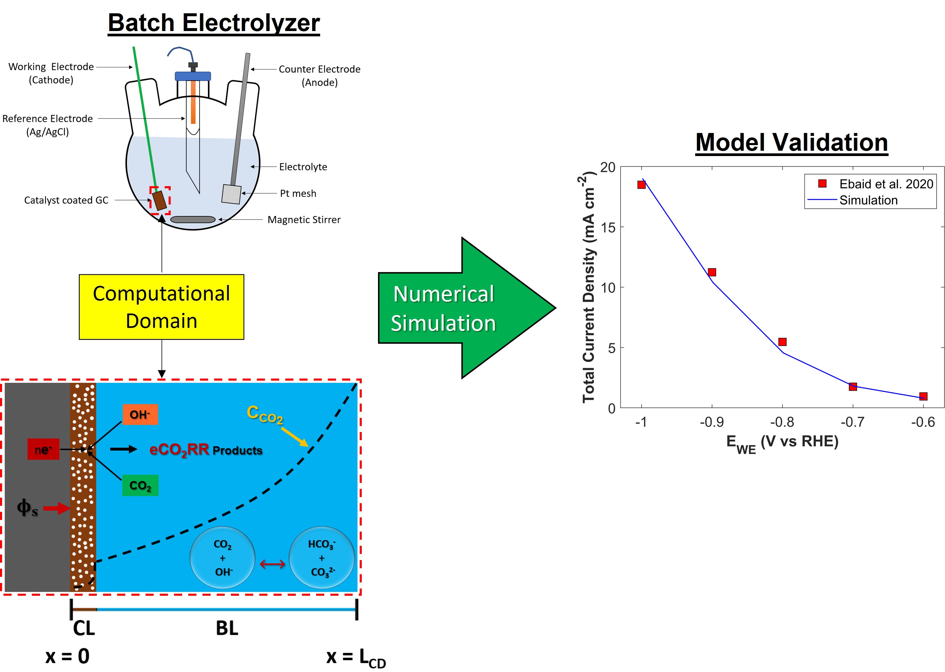
The region of interest for numerical modeling in batch-cell is the WE of GCE, where CO2 is reduced. GCE has a solid flat surface, coated with CL. Boundary layer is formed on the surface of catalyst that governs mass transfer of species between bulk of an electrolyte and WE, while bulk of an electrolyte achieves uniformity due to constant stirring. Therefore, computational domain for GCE has two important regions: porous CL, and boundary layer. A schematic of one-dimensional (1-D) computational domain is shown in the Figure 1 with all the necessary boundary conditions.
A comprehensive numerical model is developed to deconvolute the physio-electrochemical phenomenon such as mass transfer due to diffusion and electromigration, charge conservation, electrochemical reaction, and chemical reactions in the computational domain. A total of 6 species have been modeled: dissolved CO2, hydroxyl ions (OH-1), bicarbonate ions (HCO31-), carbonate ions (CO32-), protons (H+), and potassium ions (K+). Catalyst used in this study reduces CO2 to five different products with higher selectivity for C2+ products: carbon mono-oxide (CO), methane (CH4), ethylene (C2H4), ethanol (C2H5OH), and propanol (C3H7OH). Alongside these products, a competing parasitic hydrogen evolution reaction (HER) also takes place. The electrochemical reaction for each of these products is given in the Table 1 [38]. It is assumed that gaseous products (H2, CO, CH4, C2H4) bubble out as soon as they are produced, while liquid phase products act as neutral species, and do not participate in any reaction. Water (H2O) is assumed to be ubiquitous species in computational domain; therefore, it is not included in the modeling. Electrolyte is a 1 M KOH solution. Besides electrochemical conversion of CO2 into useful products, a considerable amount of CO2 reacts reversibly with the hydroxyl ions (OH-1) to produce bicarbonates (HCO3-1), and carbonates (CO32-) ions. These reactions govern local pH in computational domain. Due to high pH (~1 M KOH pH=14) of an electrolyte, only the reactions in the Table 2 have been considered in the model [45]. Precipitation of bicarbonate/carbonate salts are ignored in the numerical model. Although, salt build-up has a substantial deteriorating effect on the CL [11,12] and it also increases required cell potential if experiment is carried out for extended period [10], but in case of batch-cell modeling, this phenomenon can be ignored as a fresh electrolyte solution is used for each batch-cell experiment [12].
Specie balance is used to model concentration of species in the CL, and the boundary layer.
Nj describes the molar flux of specie j in computational domain, while source terms on the right hand represents the consumption and the generation of species due to chemical and electrochemical reactions, respectively. Nernst-Planck equation is invoked for the molar flux of species in computational domain [42].
First term on the right-hand side is the diffusion of species according to Fick’s law, while the second term represents the electro-migration of charged species; therefore, the second term becomes zero for neutral species such as dissolved CO2. The diffusion of species in porous CL is corrected using Bruggeman correlation [46]. The effective diffusion coefficient () of species in porous CL depends on its porosity (), and tortuosity ().
An additional equation is required for electrolyte potential () to close the degree of freedom; therefore, electroneutrality equation is included in the model.
Nernst-Planck equation assumes dilute-solution theory [24,42]. Modeled domain is not dilute under specified conditions. Concentrated solution theory requires additional diffusion coefficients which are not available in the literature.
The chemical consumption/generation term is defined as follows:
is the stoichiometric coefficient. It is negative for reactant species, and positive for product species. and are the forward and the reverse reaction rate constants, respectively. is an equilibrium constant.
The electrochemical source term in specie balance is defined as:
The term () represents molar weight of species. is the effective surface area available for CO2 reduction in porous CL domain, represents the electron transferred in each reaction , is the partial current density (PCD), and F is the Faraday’s constant. The electrode kinetics are modeled using concentration dependent Tafel equation [47] that describes the electrochemical conversion of dissolved CO2. A detailed derivation of the Tafel equation is provided in the supplementary information. The final form of the Tafel kinetic equation used in the model is:
This formulation of Tafel kinetic equation is adopted from Bui et al. [21]. Tafel equation has several unknown parameters that are either the direct inputs to simulation or obtained through data fit to experimental findings. is the applied cell potential, while is evaluated by solving Nernst-Planck equation, and electroneutrality equation (see equation 2, and 5). is the thermodynamic potential. represents the reaction order of CO2 for specific product species. It could be obtained either through experimental data fitting of CO2 reduction at various applied potential [25] or through rigorous microkinetic modeling [44]. According to the density functional theory calculations, is the number of elementary steps in CO2 reduction towards certain product specie, which is the most simplified way to obtain this parameter. is the pH rate ordering parameter. It is estimated by fitting experimental data of current density versus pH at a given applied potential. In this study, and for all product species are sourced from the reference [21], and their values are listed in Table 4. and are local CO2 concentration, and local pH, respectively. Obtaining these values experimentally is quite challenging; hence, simulations are conducted, similar to Gupta et al. [18], using experimental inputs to determine them. is the reference concentration that is set to 1 M. is the transfer coefficient, while is the exchange current density.
Charge conservation in computational domain is modeled using the following equations.
Ohm’s law is used to define the relation between current and voltage.
represents the conductivity of solid catalyst, and liquid electrolyte. In porous CL, effective conductivity is used according to the Bruggeman correlation.
Concentration of dissolved CO2 in 1 M KOH at STP is 24.57 mM. It is estimated using Henry’s law.
In case of an electrolyte with high concentration of ions, solubility of CO2 is reduced. Reduced CO2 solubility in an electrolytic solution is evaluated using Sechenov’s constants [50].
is the Sechenov’s constant, and is the molar concentration of ions. Sechenov’s constants values are provided in Table 3.
At x=LCD, the concentration of species is set to the bulk of an electrolyte. CO2 starts diffusing from the interface of boundary layer and bulk electrolyte to reach the surface of CL, where it undergoes eCO2RR. Since CL is a porous domain, it offers more active sites for CO2 reduction, but due to intricate network of pores, diffusion of CO2 inside CL is reduced. The nature of eCO2RR products depends on the catalyst. The thickness/length of boundary layer is about 100 [21]. However, this value changes with the stirring speed (in RPM). Potential () is applied at x=0, whereas it is assumed that reference electrode (RE) is located at the interface of boundary layer and bulk electrolyte (x=LCD), where electrolyte potential is set to zero (). Moreover, steady state, and isothermal conditions have been assumed.
2.1. Kinetic Parameters from Experimental Data
In this section, Tafel equation parameters for each CO2 reduction product are obtained from the experimental data. Experimental data is provided in Table S1 (refer to supplementary information). Tafel kinetic equation discussed in the last section (see equation 9) is used to estimate kinetic parameters. Equation 9 has six unknown parameters including , , , , , . Parameter values for , and are provided in Table 4. Parameters , and are listed in Table 5. , and values are reported in Table 6.

Table 4.
List of CO2 reaction rate order parameter () and pH rate order parameter () values. Parameter values are sourced from Bui et al. [21].
Table 4.
List of CO2 reaction rate order parameter () and pH rate order parameter () values. Parameter values are sourced from Bui et al. [21].
| Product Species | ||
| H2 | 0 | 0.5 |
| CO | 1.5 | 1.56 |
| CH4 | 0.84 | 1.56 |
| C2H4 | 1.36 | 0 |
| EtOH | 0.96 | 0 |
| PrOH | 0.96 | 0 |
Local CO2 concentration, and pH values are estimated by simulating experimental data. Experimental TCD
is set as a boundary condition. Mass flux boundary condition, estimated from experimental PCD, is used for dissolved CO2 and hydroxyl ions (OH-1) species balance. In this way, local average CO2 concentration, and local average pH values are estimated in computational domain. These values are provided in Table 5.
Remaining two parameters , and are obtained through comparing with experimental data. Information provided in Table 4, and Table 5 is used to evaluate the normalized current density.
Tafel equation is simplified as:
The slope, and the intercept of the equation 22 provide , and , respectively. Normalized current density plots as a function of overpotential for each experimentally recorded CO2 reduction product are shown in Figure S3.
2.2. Numerical Model for SE and GDLE
In this section, numerical model for other two WEs have been presented: SE, and GDLE. In practical, SE is made up of a single metal such as Cu, but, in this study, it is assumed that SE is made-up of catalyst CuAg0.5Ce0.2. GDLE is a GDL paper that contains both macro pores (carbon fibers), and micro pores (carbon powder). A layer of catalyst is coated on top of micro pore layer. Electrochemical kinetic parameters obtained in the previous section are used to simulate both electrodes.
2.2.1. Solid Electrode Numerical Model
Figure 2 illustrates the 1-D computational domain of SE, which comprises solely the boundary layer. Computational domain contains six species: dissolved CO2, OH-, HCO3-, CO3=, H+, K+. Species flux is solved using equation 1. Concentration of these species is set to the bulk electrolyte values at (x=LCD). CO2 diffuses from the interface of boundary layer and bulk electrolyte (x=LCD) to reach the surface of the electrode. Electrochemical reaction happens at the surface of the electrode (x=0). Therefore, Neumann flux boundary condition is used to model the consumption and production of CO2 and OH- ions at the surface of an electrode (x=0), respectively. Potential () is applied at surface of the electrode, while electrolyte potential () is set to 0 at x=LCD, assuming that RE is placed at this location. In case of SE, length of the computational domain is similar to the thickness of the boundary layer, and the length of the computational domain is 100 m.
2.2.2. GDLE Numerical Model
GDLE consists of porous GDL and porous CL. Both GDL and CL are assumed to have a uniform structure with consistent pore size and isotropic porosity. A 1-D computational domain of GDLE is shown in Figure 3. The porous nature of the GDLE enables reactant species to diffuse from both the front side (with the CL) and the back side (without the CL). GDLE computational domain has 4 regions: two boundary layers, a porous GDL, and a porous CL. Computational domain contains dissolved CO2, OH-, HCO3-, CO3=, H+, and K+, and species transport is modeled using equation 1. Concentration of species is set to bulk on an electrolyte at x=0, and x=LCD. CO2 diffuses from both ends of the computational domain to reach CL, where it undergoes eCO2RR. GDL serves two important functions: it supports the CL and acts as a medium for electronic conductor. Potential () is applied at the interface of GDL and boundary layer. It is assumed that RE is located at x=LCD, and the electrolyte potential () at this location is set to zero.
2.3. Numerical Simulation
Numerical model developed in this study is simulated using COMSOL Multiphysics v6.1 environment. COMSOL Multiphysics uses finite element technique to discretize the differential equations. MUMPS direct general solver is used to solve set of algebraic equations (Ax=B). Total number of nodes in computational domain are 200; number of nodes in CL domain, and boundary layer domain are set to 150, and 50, respectively. Information required to simulate the model is provided in Table 6.
Grid independent study is performed to check the model consistency and robustness. CL domain is more sensitive to species concentration gradient than the boundary layer domain, as eCO2RR happens inside the pores of CL; therefore, smaller element size (0.30 m) is used in CL domain, comparing with boundary layer domain with relatively bigger element size (0.67 m). Grid independent solution is obtained when the variation in the TCD, at a fixed applied cathodic potential of -1.0 V vs RHE, goes below 1% by increasing number of nodes (decreasing element size) in computational domain. Grid independent solution is shown in Figure 4.
2.4. Numerical Model Validation
Numerical model is validated by comparing simulated TCD result with experimental data, see Figure 5. Numerical model shows good agreement with experiment, however there is a slight difference in simulated TCD slope and experimental TCD slope. Numerical model predicts TCD with positive slope, however, the slope of experimental data shows a decreasing trend with the increase in applied cathodic potential. In experiments, electrolyte saturated with CO2 is used, and batch-cell is sealed for the duration of an experiment. Concentration of dissolved CO2 in an electrolyte becomes a function of time, and the concentration of CO2, which is 24.57 mM in 1 M KOH at STP, keeps on decreasing. This physical phenomenon is not catered in the simulation, and it is simply replaced with a Dirichlet concentration boundary condition. This assumption maintains a relatively higher, and constant concentration gradient for CO2 at a certain applied cathodic potential, than the experiments where mass transfer resistance increases with decreasing CO2 concentration in the bulk electrolyte. Therefore, decreasing slope trend for experimental current density is due to scarce supply of CO2, which becomes significant at higher applied potentials. Furthermore, use of raw technique for kinetic parameter estimation, and incapability of 1-D model to fully describe underlying physics could also affect the numerical simulation results. Despite the simplification of the numerical model, it is able to predict TCD with quite a good accuracy.
A comparison of simulated PCD of eCO2RR products with experimental data is shown in Figure S4. Except for ethylene, all the individual current density shows a good match with experiment. Experimental data for ethylene shows irregular behavior, especially the data point at -0.7 V vs RHE and -1.0 V vs RHE, which are significantly away from the normal trend.
Numerical model developed in this study is also validated with the experimental data of Ebaid et al. [43]. Cu foil and graphite rod were used as a WE and counter electrode (CE), respectively. Electrolyte was 0.1 M CsHCO3 saturated with CO2. Validation results for TCD and PCD are shown in Figure 6 and Figure S5, respectively.
3. Results and Discussion
In this section, numerical model is used to study the effect of critical parameters of batch-cell with GCE using the kinetic parameters of CuAg0.5Ce0.2 catalyst. The thickness of the boundary layer is a crucial factor that governs the diffusion rate of species. Thicker boundary layer offers significant resistance to CO2 diffusion. It does not only increase diffusion time of CO2 to reach catalyst surface; the probability of CO2 consumption by side reactions also increases, even further reducing effective concentration of CO2 available for eCO2RR. Additionally, at lower cathodic potentials, an adequate amount of CO2 is available for eCO2RR. However, the TCD sharply decreases at higher cathodic potentials due to an imbalance between the rate of eCO2RR and CO2 mass transfer. The effect of boundary layer thickness on TCD at -1.0 V vs RHE is shown in the Figure 7. TCD is obtained for 4 different boundary layer thicknesses of equal interval: 40 m, 80 m, 120 m, 160 m. Figure 7 shows an inverse relationship between TCD, and boundary layer thickness, and the trend is not linear. A substantial improvement in the TCD at boundary layer thickness of 40 m, comparing with 160 m, is due to the lower resistance to CO2 mass transfer and decline in chemical conversion of CO2 into bi-carbonates and carbonates. Furthermore, average surface CO2 concertation available for eCO2RR is much higher at 40 m thick boundary layer, compared with CO2 concertation at other boundary layer thicknesses, see Figure 8. This finding is consistent with gas flow electrolyzer using GDL, where boundary layer thickness inside the CL is only a few micrometers thick, minimizing the resistance to CO2 mass transfer in aqueous phase [24]. Boundary layer thickness has a substantial impact on the movement of other species, such OH-1 ions that governs pH in the vicinity of WE, and hence the selectively of eCO2RR products [54]. Thinner boundary layer expedites the transport of OH-1ions from the surface of CL to the bulk of an electrolyte. It is evident from Figure 8, where pH of 14.23 at boundary layer thickness of 160 m drops to 14.08 at boundary layer thickness of 40 m.
CL has a porous structure. Its porosity is defined as [24]:
is the catalyst mass per unit area, is the catalyst mass density, and is the thickness of CL. Porous CL offers more active sites for eCO2RR, than a traditional single metal solid electrode [24]. Although porous CL has more active surface area, it also minimizes catalyst loading (if the CL length is kept constant, see equation 23), which affects the TCD. Porous CL accelerates species diffusion rate; allows more CO2 to penetrate inside CL, and the removal of product species from CL to the bulk of an electrolyte. CL has pore sizes in the range 10 – 100 nm [27]. The effect of CL porosity on TCD is plotted in Figure 9. TCD rises gradually from 50.48 mA cm-2 to 114.32 mA cm-2, when CL porosity is reduced from 0.8 to 0.3. The increase in TCD with reduced CL porosity is due to increase in catalyst mass loading that substantially increases active sites for CO2 reduction. However, lower CL porosity affects CO2 diffusion rate and increases the probability of CO2 carbonation. Therefore, the average CO2 concentration is lower in CL with lower porosity value, see Figure 10.
CL thickness, and CL porosity have a direct link with each other, see equation 23. Desired CL thickness with required CL porosity may be obtained by adjusting the catalyst loading. CL thickness plays a vital role in electrochemical kinetics. Although thicker CL seems to have increased catalyst loading, which could have a substantial impact on TCD; ironically, most part of the CL is rendered inoperable due to limited supply of CO2, and fast CO2 reduction kinetics. Moreover, thicker CL has longer tortuous diffusion path, reducing species diffusion rate inside CL. Figure 11 shows that TCD increases by reducing CL thickness. TCD with 20 m thick CL is 71.13 mA cm-2, and TCD with 3 m thick CL is 93.28 mA cm-2, approximately. A total increase of 24 mA cm-2 is observed just by varying the CL thickness, keeping all other parameters constant. This increase in TCD is attributed to improvement in species diffusion rate. Additionally, average surface CO2 concentration increases with decreasing CL thickness, due to shorter diffusion path inside CL, see Figure 12. Local distribution of CO2 in computational domain (boundary layer + CL) shows that CO2 concertation decreases gradually from the outer periphery of boundary layer to the interface of boundary layer and CL, but a sharp decline in CO2 concertation profile is seen when CO2 enters into the CL domain, see Figure 13. Local CO2 concentration profile in CL shows that most CO2 gets consumed before even reaching the middle of the CL. Because in boundary layer CO2 undergoes a reversible chemical reaction, whereas in the CL, CO2 is not only chemically converted but also consumed electrochemically.
Nature of an electrolyte has a significant impact on CO2 reduction kinetics. KOH is widely recognized as one of the most effective electrolytes for CO2 reduction, owing to its high ionic conductivity and alkaline properties, which help suppress HER [12,14,55,56,57,58]. Potassium bicarbonate (KHCO3), a buffer solution, is known for providing near neutral pH conditions for CO2 reduction [24,25]. To analyze the effect of nature of an electrolyte on CO2 reduction kinetics, 1 M KHCO3 electrolyte is simulated, and compared with 1 M KOH simulation results, see Figure 14. Two additional chemical reactions have been included in the model for 1 M KHCO3 electrolyte, see Table 7. Kinetic rate parameters for these reactions are reported in Table 6.
There is a significant difference between the TCD obtained using KHCO3 electrolyte and KOH electrolyte. The maximum TCD with KHCO3 is 101.75 mA cm-2 at an applied cathodic potential of -1.1 V vs RHE, while TCD with KOH at -1.1 V vs RHE is 116.94 mA cm-2. This difference is due to the intrinsic nature of the electrolytic solutions. KHCO3 is a buffer solution, therefore, to maintain the buffer it consumes more CO2. A batch cell, already constrained by limited CO2 supply, experiences a CO2 shortage in the CL domain, leading to a lower TCD. A comparison of average surface CO2 concentration for both electrolytes is shown in the Figure 15. Although the CO2 concentration in both cases exhibits the same trend with increasing applied potential, there is an order of magnitude difference in CO2 concentration. PCDs of CO2 reduction products using 1 M KHCO3 electrolyte are shown in Figure 16. It shows that electrolyte could alter the selectivity of eCO2RR products.
The primary purpose of an electrolyte is to enhance conductivity of an aqueous phase. An electrolyte with higher molarity provides a more conductive medium by minimizing charge transfer resistance between the electrodes [45] and by reducing the negative overpotential of CO2 reduction products [10]. Effect of KOH electrolyte strength on TCD at -1.0 V vs RHE is shown in Figure 17. TCD increases with rising electrolyte molarity but begins to plateau at significantly higher molarity levels. TCD increases as the enhanced medium conductivity facilitates the movement of charged species, thereby accelerating electrochemical kinetics. The bending of the slope at higher molarity values is attributed to the limited availability of CO2 for eCO2RR, see Figure 18. On one hand, KOH with higher molarity results in increased TCD; however, the higher concentration of OH⁻ ions consume more CO2, leading to a reduction in carbon efficiency.
TCD comparison of SE, GDLE, and GCE is shown in Figure 19. There is a stark difference between TCD of SE, and the electrodes with porous structure (GDLE, GCE). TCD of SE increases with the increase in applied cathodic potential, however, the increase is not significant, in comparison with the porous electrodes. At -0.7 V vs RHE, TCD of SE is 73.94 mA cm-2, and it rises to 77.34 mA cm-2, at -1.1 V vs RHE. There is barely an increase of 3.39 mA cm-2 in TCD. Furthermore, the slope of TCD curve for SE decreases with the increase in applied cathodic potential, because the availability of active surface area for CO2 reduction becomes a limiting factor. Average surface CO2 concentration for SE is relatively much higher compared with GDLE, and GCE, due to the limited active surface area for eCO2RR, see Figure 20. TCD of GDLE traces the GCE curve, however, GDLE has a slightly higher TCD, as it facilitates more CO2 to diffuse into CL. Also, average surface CO2 concentration is higher for GDLE than GCE.
4. Conclusion
In conclusion, we have developed a numerical model to study CO2 reduction reaction in a batch-cell with three different WEs (SE, GCE, GDLE). Numerical model is simulated using COMSOL Multiphysics software. The key conclusions derived from our numerical simulation are as follows.
- Thickness of boundary layer has an inverse relation with the TCD. Thicker boundary layer offers more resistance to CO2 diffusion, while thinner boundary layer improves the mass transfer of the species. Magnetic stirrer speed could be manipulated to control the boundary layer thickness in a batch-cell.
- CL porosity also demonstrates an inverse relation with TCD; higher the CL porosity, lower the TCD will be, and vice versa. However, higher CL porosity reduces the mass transfer resistance. An optimum selection of CL porosity is required to balance the effective diffusion rate with good TCD.
- CL thickness has a significant effect on the performance of the batch-cell. A thinner CL is much more effective in terms of current density, compared with a relatively thicker CL. Batch-cell suffers from poor CO2 diffusion rate, and limited amount of CO2 is available for eCO2RR, therefore, only a small portion of CL is used in eCO2RR. A thinner CL saves catalyst, improves species mass transfer rate, and results in a higher current density. An optimum balance of catalyst loading, CL thickness, and CL porosity could enhance the overall cell performance.
- Electrolyte nature impacts the CO2 reduction reaction. 1 M KOH performs well in comparison with 1 M KHCO3 in a batch-cell. KHCO3 is a buffer solution, therefore, it consumes relatively more CO2 to maintain its buffer. Hence, KOH is an optimum choice, as it provides a strong alkaline environment that mitigates the probability of HER.
- KOH electrolyte with higher molarity increases the TCD by minimizing the charge transfer resistance between the electrodes. Nevertheless, high molarity of KOH increases the chemical conversion of CO2 into bi-carbonates, and carbonates. An optimum distance between the electrodes could eliminate the requirement of high molar electrolyte for conductivity improvement.
- Among the three electrodes, GDLE and GCE out-perform SE in terms of current density. In particular, the porous structure of GDLE facilitates more CO2 into the CL that increases the rate of eCO2RR.
Supplementary Materials
The following supporting information can be downloaded at the website of this paper posted on Preprints.org
Author Contributions
Conceptualization, Ahmad Ijaz; Data curation, Mohammadreza Esmaeilirad; Formal analysis, Ahmad Ijaz; Funding acquisition, Mohammad Asadi and Hamid Arastoopour; Project administration, Hamid Arastoopour; Resources, SeyedSepehr Mostafayi and Mohammadreza Esmaeilirad; Supervision, Mohammad Asadi, Javad Abbasian and Hamid Arastoopour; Validation, Ahmad Ijaz; Writing – original draft, Ahmad Ijaz; Writing – review & editing, Mohammad Asadi, Javad Abbasian and Hamid Arastoopour.
Acknowledgments
This work was supported by Advanced Research Projects Agency-Energy (ARPA-E) OPEN2021 (DE-AR0001581). The views and opinions of authors expressed herein do not necessarily state or reflect those of the United States Government or any agency thereof.
Nomenclature
| mol m2s-1 | Molar flux of liquid-phase specie j | |
| m2 s-1 | Diffusion coefficient of liquid-phase specie j | |
| mol m-3 | Concentration of species j | |
| - | Charge number of species j | |
| F | C mol-1 | Faraday’s constant |
| R | J mol-1K-1 | Universal gas constant |
| T | K | Batch-cell operating temperature |
| V vs RHE | Electrolyte potential | |
| m2 s-1 | Effective diffusion coefficient of species j | |
| - | Porosity of catalyst layer | |
| - | Tortuosity of catalyst layer | |
| mol m-3s-1 | Reversible chemical reaction source term | |
| - | Stoichiometric coefficient of species j in reaction n | |
| - | Rate constant for forward reaction in reaction n | |
| - | Rate constant for reverse reaction in reaction n | |
| - | Equilibrium constant for reaction n | |
| kg mol-1 | Molar weight of species j | |
| mol m-3s-1 | Electrochemical reaction source term | |
| m-1 | Effective surface area in porous medium | |
| mA cm-2 | Partial current density for reaction k | |
| - | Number of electrons transferred in reaction k | |
| mA cm-2 | Pre-factor term for reaction k | |
| - | Transfer coefficient for reaction k | |
| V vs RHE | Overpotential for reaction k | |
| mA cm-2 | Exchange current density for reaction k | |
| mol m-3 | Local concentration of CO2 | |
| mol m-3 | Reference concentration of CO2 | |
| - | CO2 reaction rate order parameter for reaction k | |
| - | pH rate ordering parameter for reaction k | |
| pH | - | Local pH value |
| V vs RHE | Applied cathodic potential | |
| V vs RHE | Thermodynamic equilibrium potential for reaction k | |
| S | C m-3s-1 | Source term for charge conservation equation |
| S m-1 | Conductivity of medium | |
| mol m-3 | Concentration of CO2 in aqueous phase | |
| mol m-3 | Concentration of CO2 in gas phase | |
| mol m-3atm-1 | Henry’s constant for CO2 | |
| m3 mol-1 | Sechenov’s constant | |
| mol m-3 | Molar concentration of ions | |
| - | Sechenov’s equation parameters | |
| - | ||
| - | ||
| - | ||
| kg m-2 | Catalyst loading per unit area | |
| kg m-3 | Catalyst density | |
| m | Catalyst layer thickness | |
| Abbreviations | ||
| eCO2RR | Electrochemical CO2 reduction reaction | |
| GDL | Gas diffusion layer | |
| GDE | Gas diffusion electrode | |
| MEA | Membrane electrode assembly | |
| GDLE | Gas diffusion layer electrode | |
| GCE | Glassy carbon electrode | |
| WE | Working electrode | |
| CE | Counter electrode | |
| RE | Reference electrode | |
| SE | Solid electrode | |
| CL | Catalyst layer | |
| TCD | Total current density | |
| CD | Computational domain | |
| PCD | Partial current density | |
| HER | Hydrogen evolution reaction | |
References
- (2023) IEA (2023), World Energy Outlook 2023. IEA, Paris, License: CC BY 4.0 (report); CC BY NC SA 4.
- Calvin K, Dasgupta D, Krinner G, et al. (2023) IPCC, 2023: Climate Change 2023: Synthesis Report. Contribution of Working Groups I, II and III to the Sixth Assessment Report of the Intergovernmental Panel on Climate Change [Core Writing Team, H. Lee and J. Romero (eds.)]. IPCC, Geneva, Switzerland.
- Jos Olivier (2022) Trends in Global CO2 and Total Greenhouse Gas Emissions; 2021 Summary Report. PBL Netherlands Environmental Assessment Agency.
- Arastoopour H (2019) The critical contribution of chemical engineering to a pathway to sustainability. Chem Eng Sci 203:247–258. [CrossRef]
- Zhang X, Guo S-X, Gandionco KA, et al. (2020) Electrocatalytic carbon dioxide reduction: from fundamental principles to catalyst design. Mater Today Adv 7:100074. [CrossRef]
- Wu W, Lu Q, Li G, Wang Y (2023) How to extract kinetic information from Tafel analysis in electrocatalysis. J Chem Phys 159:. [CrossRef]
- Weekes DM, Salvatore DA, Reyes A, et al. (2018) Electrolytic CO2 Reduction in a Flow Cell. Acc Chem Res 51:910–918. [CrossRef]
- Lin R, Guo J, Li X, et al. (2020) Electrochemical Reactors for CO2 Conversion. Catalysts 10:473. [CrossRef]
- Wakerley D, Lamaison S, Wicks J, et al. (2022) Gas diffusion electrodes, reactor designs and key metrics of low-temperature CO2 electrolysers. Nature Energy 2022 7:2 7:130–143. [CrossRef]
- Rabinowitz JA, Kanan MW (2020) The future of low-temperature carbon dioxide electrolysis depends on solving one basic problem. Nat Commun 11:5231. [CrossRef]
- Kim JY ‘Timothy,’ Zhu P, Chen F-Y, et al. (2022) Recovering carbon losses in CO2 electrolysis using a solid electrolyte reactor. Nat Catal 5:288–299. [CrossRef]
- Sassenburg M, Kelly M, Subramanian S, et al. (2023) Zero-Gap Electrochemical CO2 Reduction Cells: Challenges and Operational Strategies for Prevention of Salt Precipitation. ACS Energy Lett 8:321–331. [CrossRef]
- Mardle P, Cassegrain S, Habibzadeh F, et al. (2021) Carbonate Ion Crossover in Zero-Gap, KOH Anolyte CO2 Electrolysis. Journal of Physical Chemistry C 125:25446–25454. [CrossRef]
- Reyes A, Jansonius RP, Mowbray BAW, et al. (2020) Managing Hydration at the Cathode Enables Efficient CO2Electrolysis at Commercially Relevant Current Densities. ACS Energy Lett 5:1612–1618. [CrossRef]
- Wheeler DG, Mowbray BAW, Reyes A, et al. (2020) Quantification of water transport in a CO2 electrolyzer. Energy Environ Sci 13:5126–5134. [CrossRef]
- Wu H, Li X, Berg P (2009) On the modeling of water transport in polymer electrolyte membrane fuel cells. Electrochim Acta 54:6913–6927. [CrossRef]
- Baumgartner LM, Goryachev A, Koopman CI, et al. (2023) Electrowetting limits electrochemical CO2 reduction in carbon-free gas diffusion electrodes. Energy Advances. [CrossRef]
- Gupta N, Gattrell M, MacDougall B (2006) Calculation for the cathode surface concentrations in the electrochemical reduction of CO2 in KHCO3 solutions. J Appl Electrochem 36:161–172. [CrossRef]
- Hashiba H, Weng LC, Chen Y, et al. (2018) Effects of electrolyte buffer capacity on surface reactant species and the reaction rate of CO2 in Electrochemical CO2 reduction. Journal of Physical Chemistry C 122:3719–3726. [CrossRef]
- Corpus KRM, Bui JC, Limaye AM, et al. (2023) Coupling covariance matrix adaptation with continuum modeling for determination of kinetic parameters associated with electrochemical CO2 reduction. Joule 7:1289–1307. [CrossRef]
- Bui JC, Kim C, Weber AZ, Bell AT (2021) Dynamic Boundary Layer Simulation of Pulsed CO2 Electrolysis on a Copper Catalyst. ACS Energy Lett 6:1181–1188. [CrossRef]
- Qiu H, Wang F, Liu Y, Guo L (2023) Improved product selectivity of electrochemical reduction of carbon dioxide by tuning local carbon dioxide concentration with multiphysics models. Environ Chem Lett 21:3045–3054. [CrossRef]
- Whipple DT, Finke EC, Kenis PJA (2010) Microfluidic reactor for the electrochemical reduction of carbon dioxide: The effect of pH. Electrochemical and Solid-State Letters 13:B109. [CrossRef]
- Weng LC, Bell AT, Weber AZ (2018) Modeling gas-diffusion electrodes for CO2 reduction. Physical Chemistry Chemical Physics 20:16973–16984. [CrossRef]
- Weng LC, Bell AT, Weber AZ (2019) Towards membrane-electrode assembly systems for CO2 reduction: a modeling study. Energy Environ Sci 12:1950–1968. [CrossRef]
- Weng LC, Bell AT, Weber AZ (2020) A systematic analysis of Cu-based membrane-electrode assemblies for CO2 reduction through multiphysics simulation. Energy Environ Sci 13:3592–3606. [CrossRef]
- Kas R, Star AG, Yang K, et al. (2021) Along the Channel Gradients Impact on the Spatioactivity of Gas Diffusion Electrodes at High Conversions during CO2 Electroreduction. ACS Sustain Chem Eng 9:1286–1296. [CrossRef]
- Ehlinger VM, Lee DU, Lin TY, et al. (2024) Modeling Planar Electrodes and Zero-Gap Membrane Electrode Assemblies for CO 2 Electrolysis. ChemElectroChem 11:. [CrossRef]
- Gabardo CM, O’Brien CP, Edwards JP, et al. (2019) Continuous Carbon Dioxide Electroreduction to Concentrated Multi-carbon Products Using a Membrane Electrode Assembly. Joule 3:2777–2791. [CrossRef]
- Yang SH, Jung W, Lee H, et al. (2023) Membrane Engineering Reveals Descriptors of CO 2 Electroreduction in an Electrolyzer. ACS Energy Lett 8:1976–1984. [CrossRef]
- Choi W, Park S, Jung W, et al. (2022) Origin of Hydrogen Incorporated into Ethylene during Electrochemical CO 2 Reduction in Membrane Electrode Assembly. ACS Energy Lett 7:939–945. [CrossRef]
- Bui JC, Lees EW, Pant LM, et al. (2022) Continuum Modeling of Porous Electrodes for Electrochemical Synthesis. Chem Rev 122:11022–11084. [CrossRef]
- Brée LC, Wessling M, Mitsos A (2020) Modular modeling of electrochemical reactors: Comparison of CO2-electolyzers. Comput Chem Eng 139:106890. [CrossRef]
- Subramanian S, Yang K, Li M, et al. (2023) Geometric Catalyst Utilization in Zero-Gap CO 2 Electrolyzers. ACS Energy Lett 8:222–229. [CrossRef]
- Dunne H, Liu W, Ghaani MR, et al. (2024) Sensitivity Analysis of One-Dimensional Multiphysics Simulation of CO 2 Electrolysis Cell. The Journal of Physical Chemistry C 128:11131–11144. [CrossRef]
- Ijaz A, Mostafayi S, Asadi M, et al. (2024) Two-Dimensional Steady State Numerical Simulation of Electrochemical CO2 Conversion Using a Zero-Gap Electrolyzer. 2: In, 2024.
- Mostafayi S, Ijaz A, Amouzesh SP, et al. (2024) A Multiphase CFD Model for Electrochemical CO2 Conversion in a Zero-Gap Membrane-Electrode Assembly Electrolyzer. 2: In, 2024.
- Fan L, Xia C, Yang F, et al. (2020) Strategies in catalysts and electrolyzer design for electrochemical CO2 reduction toward C2+ products. Sci Adv 6:. [CrossRef]
- Nitopi S, Bertheussen E, Scott SB, et al. (2019) Progress and Perspectives of Electrochemical CO2 Reduction on Copper in Aqueous Electrolyte. Chem Rev 119:7610–7672. [CrossRef]
- Lin J, Zhang Y, Xu P, Chen L (2023) CO2 electrolysis: Advances and challenges in electrocatalyst engineering and reactor design. Materials Reports: Energy 3:100194. [CrossRef]
- Arastoopour H, Gidaspow D, Lyczkowski RW (2022) Transport Phenomena in Multiphase Systems. [CrossRef]
- Newman J, Thomas-Alyea KE (2012) Electrochemical Systems, 3rd ed.
- Ebaid M, Jiang K, Zhang Z, et al. (2020) Production of C2 /C3 Oxygenates from Planar Copper Nitride-Derived Mesoporous Copper via Electrochemical Reduction of CO2. Chemistry of Materials 32:3304–3311. [CrossRef]
- Rae K, Corpus M, Bui JC, et al. (2022) Beyond Tafel Analysis for Electrochemical CO2 Reduction. [CrossRef]
- García de Arquer FP, Dinh CT, Ozden A, et al. (2020) CO2 electrolysis to multicarbon products at activities greater than 1 A cm−2. Science (1979) 367:661–666. [CrossRef]
- Das PK, Li X, Liu Z-S (2010) Effective transport coefficients in PEM fuel cell catalyst and gas diffusion layers: Beyond Bruggeman approximation. Appl Energy 87:2785–2796. [CrossRef]
- Dickinson EJF, Wain AJ (2020) The Butler-Volmer equation in electrochemical theory: Origins, value, and practical application. Journal of Electroanalytical Chemistry 872:114145. [CrossRef]
- Huang JE, Li F, Ozden A, et al. (2021) CO2 electrolysis to multicarbon products in strong acid. Science (1979) 372:1074–1078. [CrossRef]
- Sander R (2023) Compilation of Henry’s law constants (version 5.0.0) for water as solvent. Atmos Chem Phys 23:10901–12440. [CrossRef]
- Weisenberger S, Schumpe A (1996) Estimation of gas solubilities in salt solutions at temperatures from 273 K to 363 K. AIChE Journal 42:298–300. [CrossRef]
- Craig NP (2013) Electrochemical Behavior of Bipolar Membranes.
- Zeebe RE (2011) On the molecular diffusion coefficients of dissolved CO2,HCO3-, and CO32- and their dependence on isotopic mass. Geochim Cosmochim Acta 75:2483–2498. [CrossRef]
- (1977) CRC Handbook of Chemistry and Physics, 57th Edition. Soil Science Society of America Journal 41:vi–vi. [CrossRef]
- Gorthy S, Verma S, Sinha N, et al. (2023) Theoretical Insights into the Effects of KOH Concentration and the Role of OH– in the Electrocatalytic Reduction of CO2 on Au. ACS Catal 12924–12940. [CrossRef]
- Blake JW, Konderla V, Baumgartner LM, et al. (2023) Inhomogeneities in the Catholyte Channel Limit the Upscaling of CO2 Flow Electrolysers. ACS Sustain Chem Eng 11:2840–2852. [CrossRef]
- Cofell ER, Nwabara UO, Bhargava SS, et al. (2021) Investigation of Electrolyte-Dependent Carbonate Formation on Gas Diffusion Electrodes for CO2Electrolysis. ACS Appl Mater Interfaces 13:15132–15142. [CrossRef]
- Xiong H, Li J, Wu D, et al. (2023) Benchmarking of commercial Cu catalysts in CO2 electro-reduction using a gas-diffusion type microfluidic flow electrolyzer. Chemical Communications 59:5615–5618. [CrossRef]
- Li Z, Zhang T, Raj J, et al. (2023) Revisiting Reaction Kinetics of CO Electroreduction to C2+ Products in a Flow Electrolyzer. Energy and Fuels 37:7904–7910. [CrossRef]
Figure 1.
Computational domain of GCE with necessary boundary conditions.

Figure 2.
A 1-D computational domain of solid electrode with necessary boundary conditions.
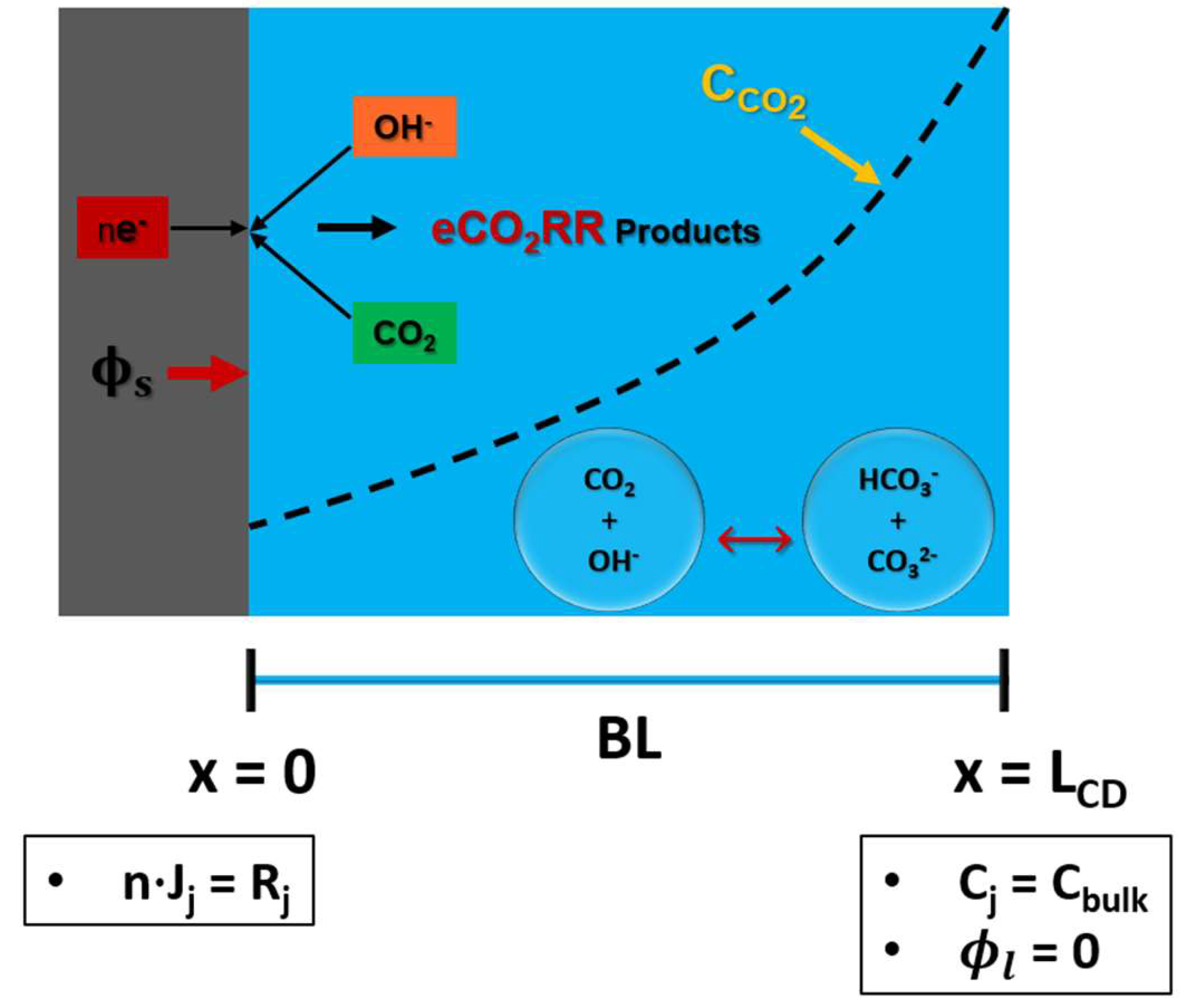
Figure 3.
A 1-D computational domain of GDLE with boundary conditions.
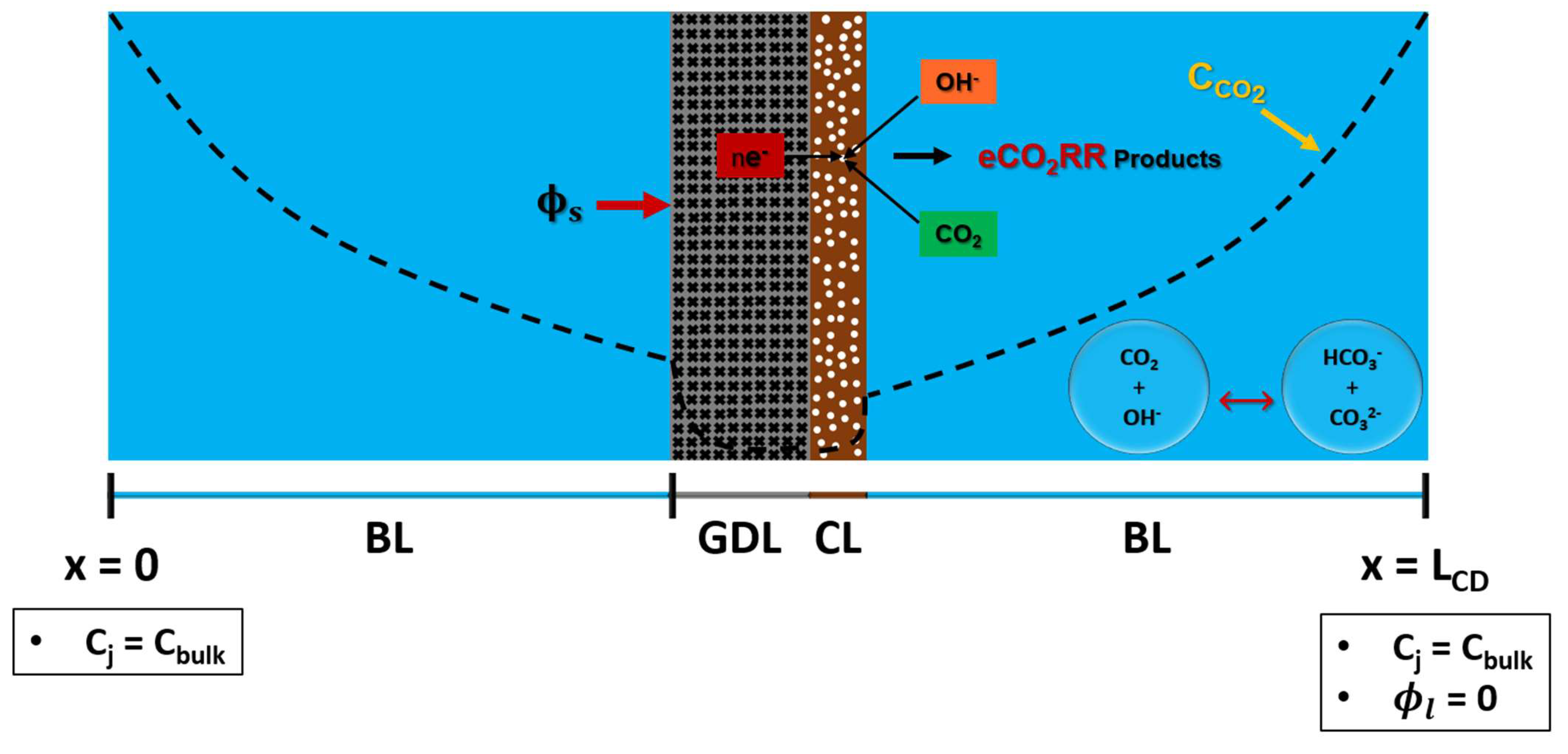
Figure 4.
A grid independence study analyzing total current density as a function of mesh nodes (elements) at a cathodic potential of -1.0 V vs RHE.
Figure 4.
A grid independence study analyzing total current density as a function of mesh nodes (elements) at a cathodic potential of -1.0 V vs RHE.
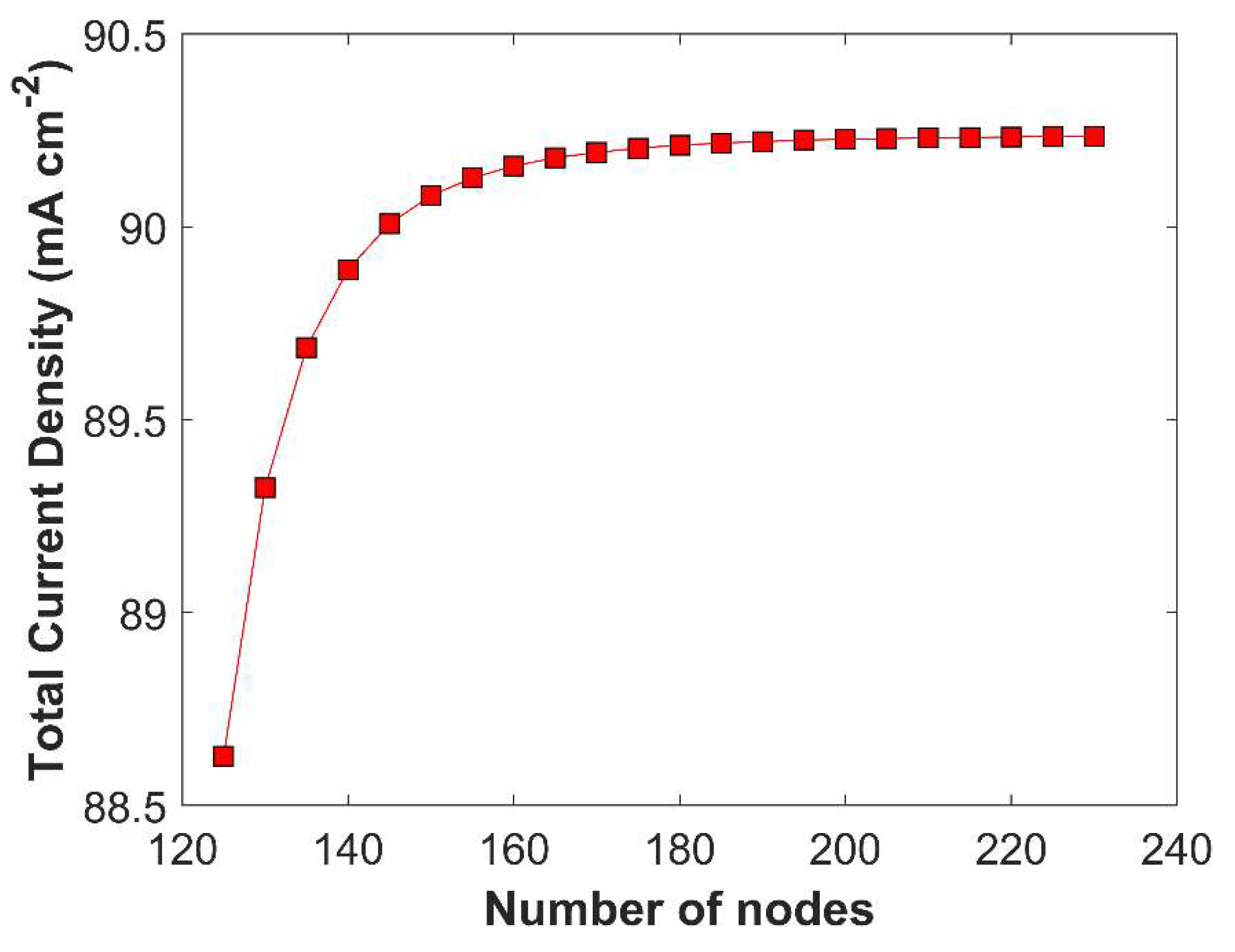
Figure 5.
Batch-cell model validation result comparing simulated TCD vs experimental TCD for CuAg0.5Ce0.2 catalyst as a function of applied cathodic potential.
Figure 5.
Batch-cell model validation result comparing simulated TCD vs experimental TCD for CuAg0.5Ce0.2 catalyst as a function of applied cathodic potential.

Figure 6.
Numerical model validation with metallic Cu catalyst.
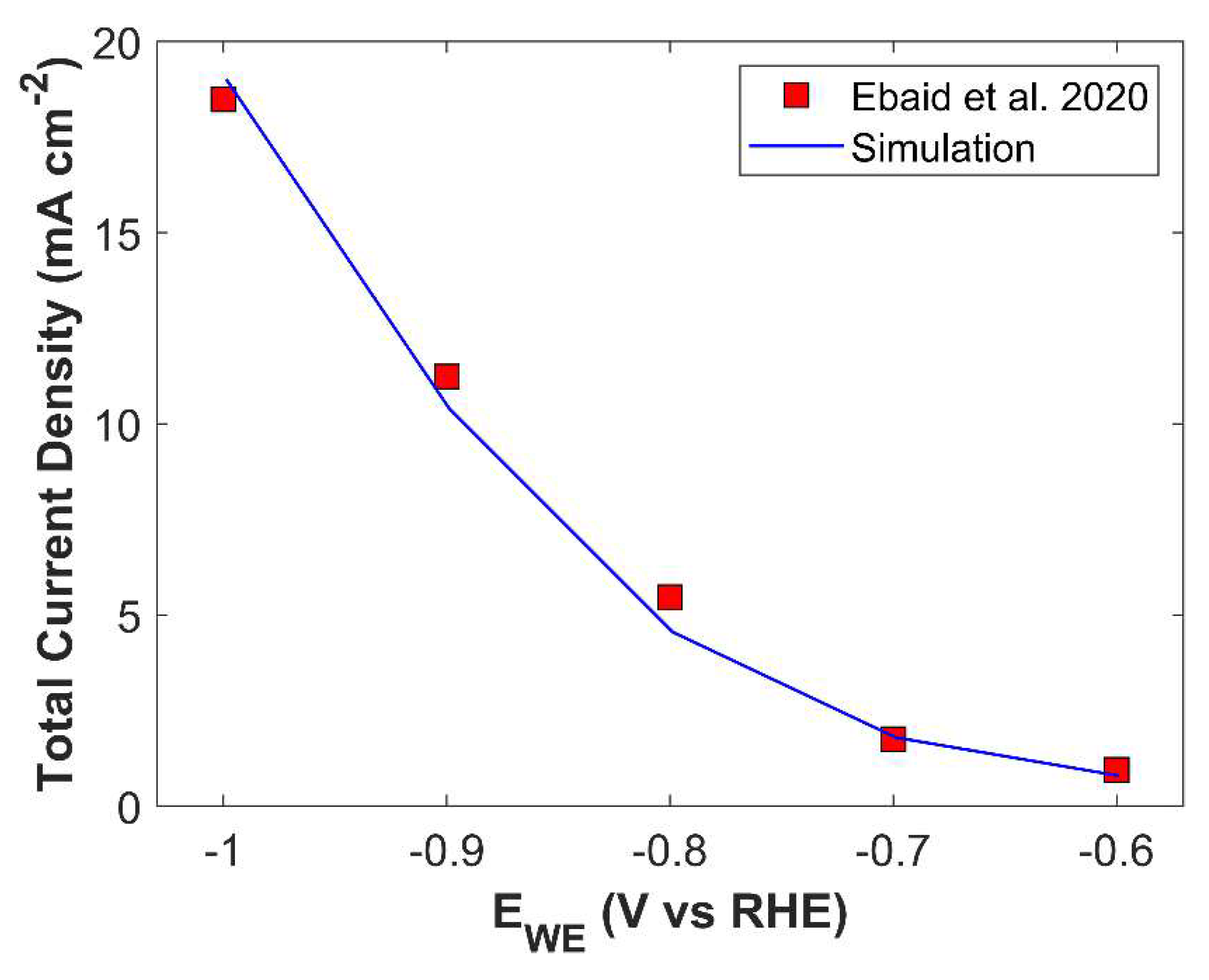
Figure 7.
Boundary layer thickness effect on TCD at a fixed applied potential of -1.0 V vs RHE.
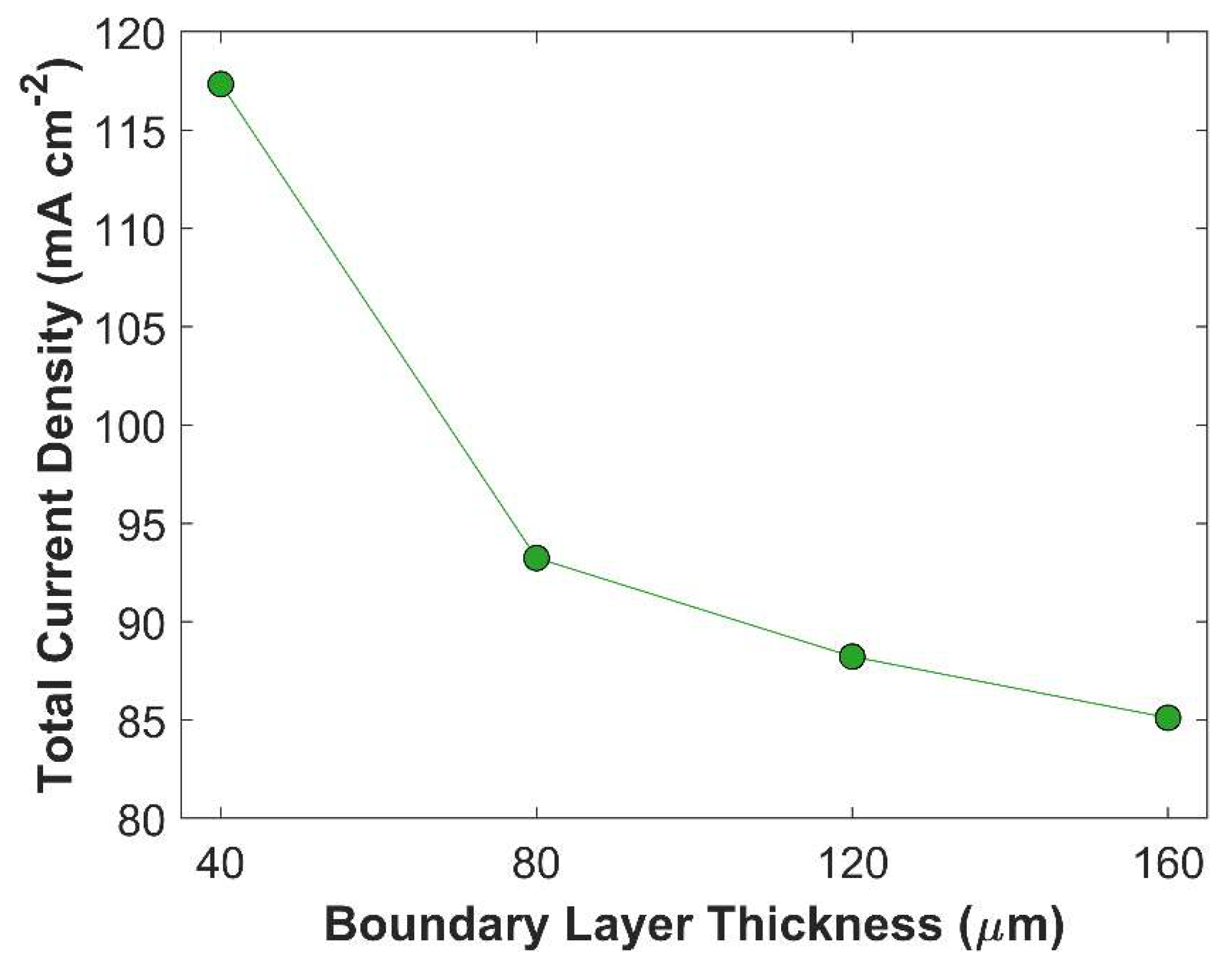
Figure 8.
Average surface CO2 concentration and pH in CL as a function of boundary layer thickness at an applied potential of -1.0 V vs RHE.
Figure 8.
Average surface CO2 concentration and pH in CL as a function of boundary layer thickness at an applied potential of -1.0 V vs RHE.
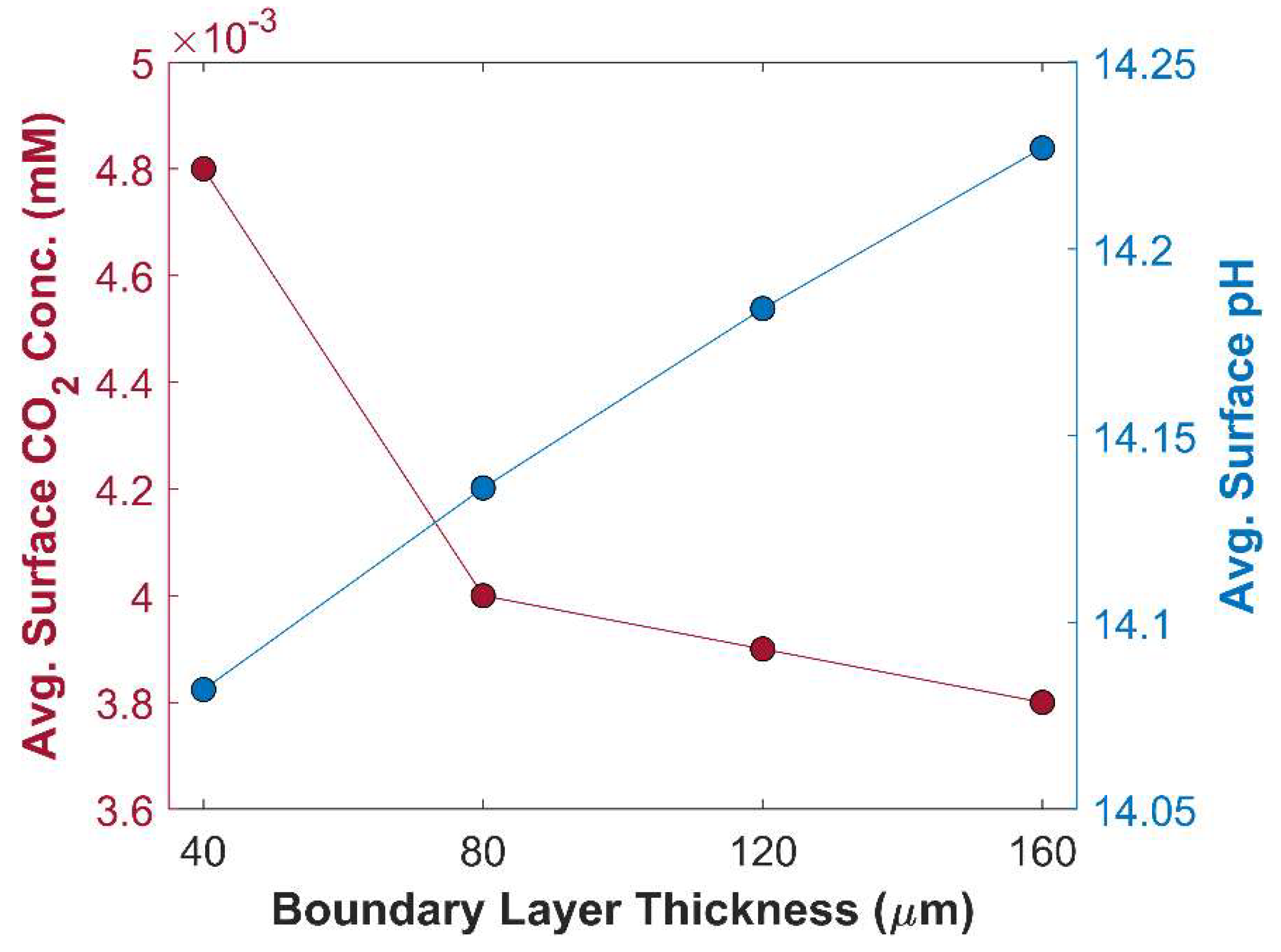
Figure 9.
Effect of CL porosity on TCD. Applied cathodic potential is -1.0 V vs RHE.
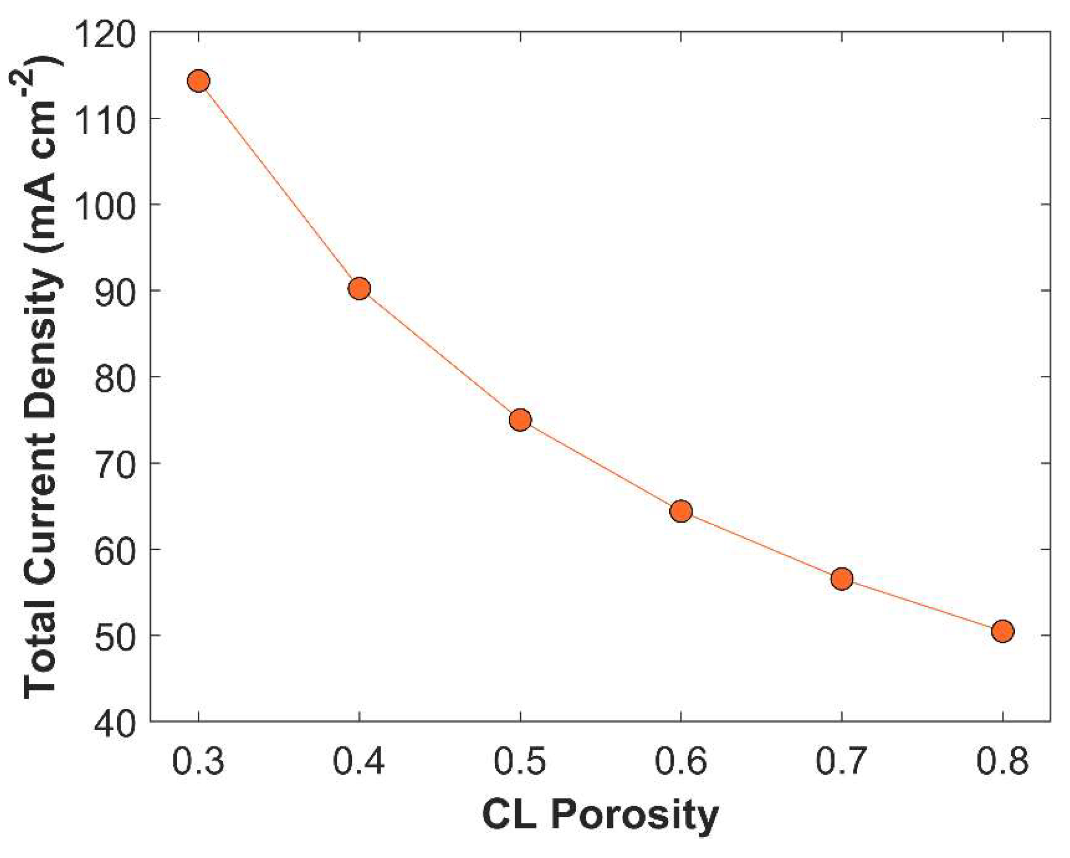
Figure 10.
Variation of average surface CO2 concentration in CL with CL porosity. Applied cathodic potential -1.0 V vs RHE.
Figure 10.
Variation of average surface CO2 concentration in CL with CL porosity. Applied cathodic potential -1.0 V vs RHE.
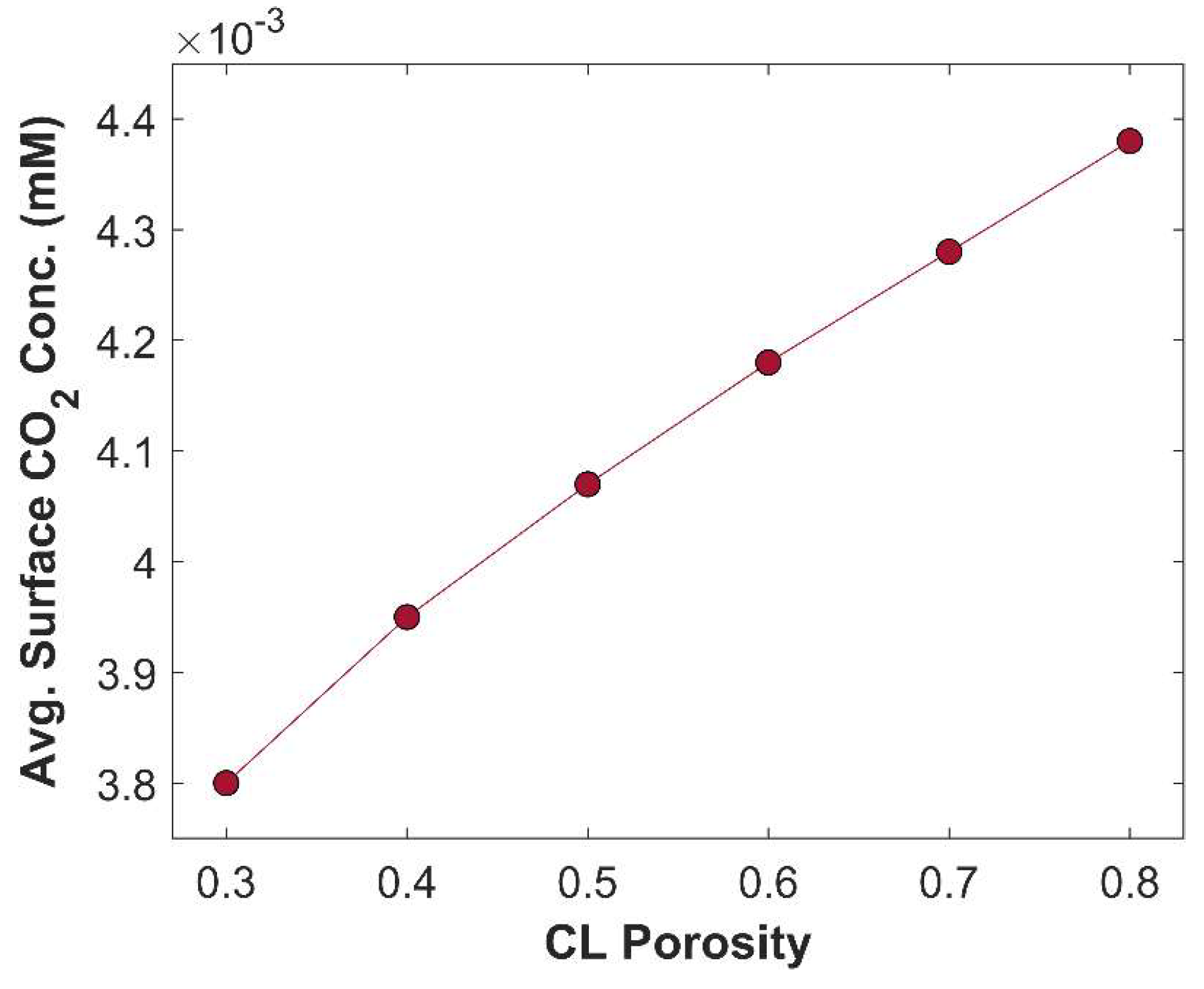
Figure 11.
Variation of TCD with CL thickness. Applied cathodic potential is -1.0 V vs RHE.
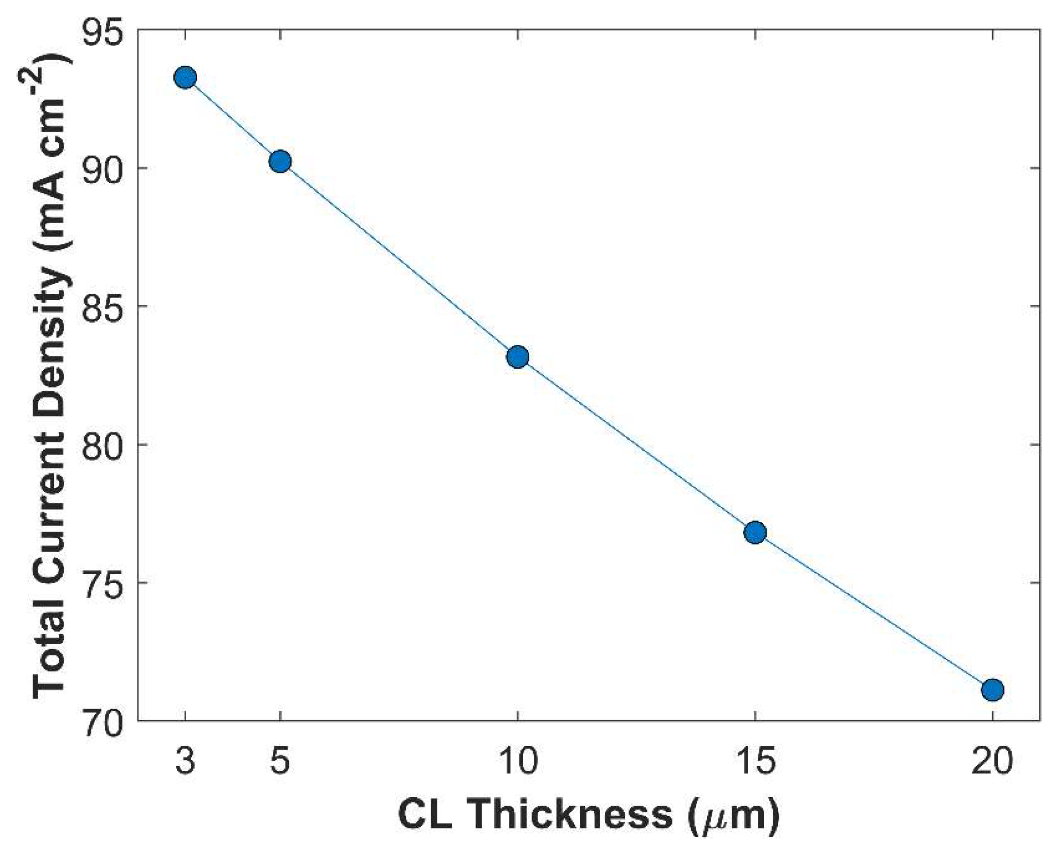
Figure 12.
Average surface CO2 concentration versus CL thickness. Applied cathodic potential is -1 V vs RHE.
Figure 12.
Average surface CO2 concentration versus CL thickness. Applied cathodic potential is -1 V vs RHE.
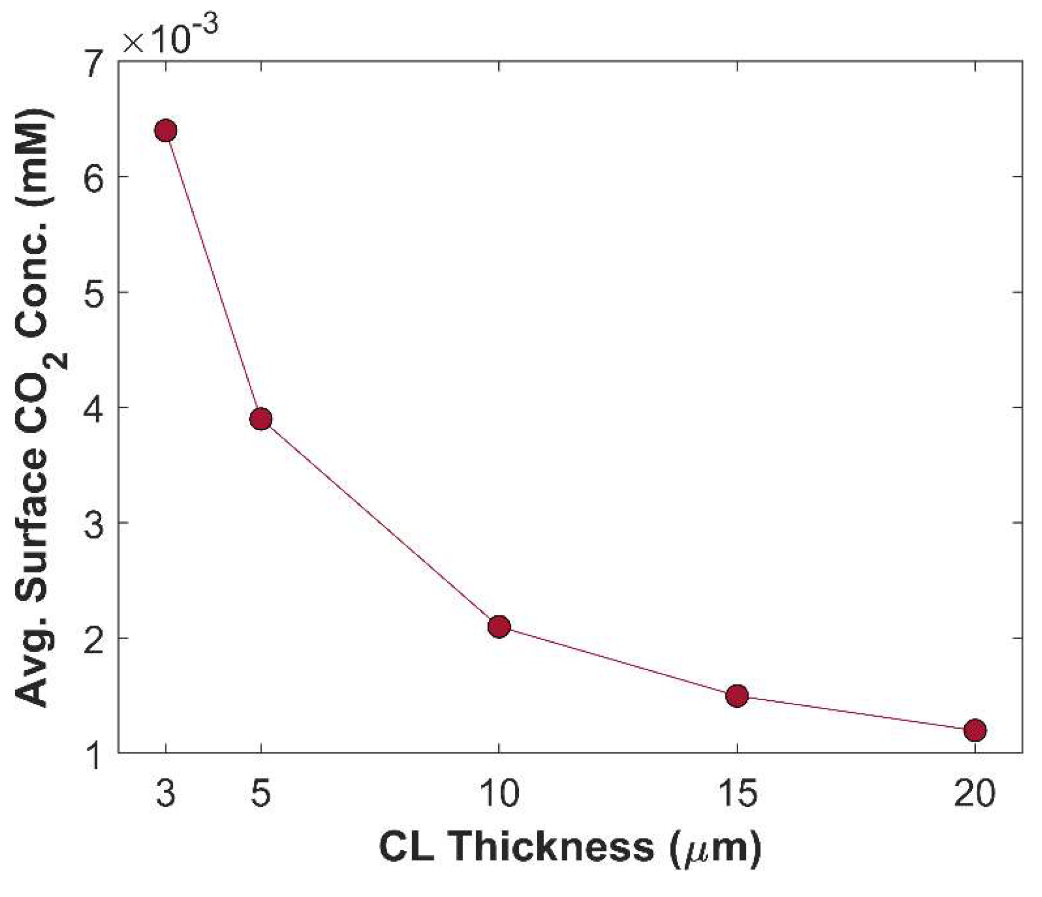
Figure 13.
Local CO2 concentration profile in computational domain (boundary layer +CL).
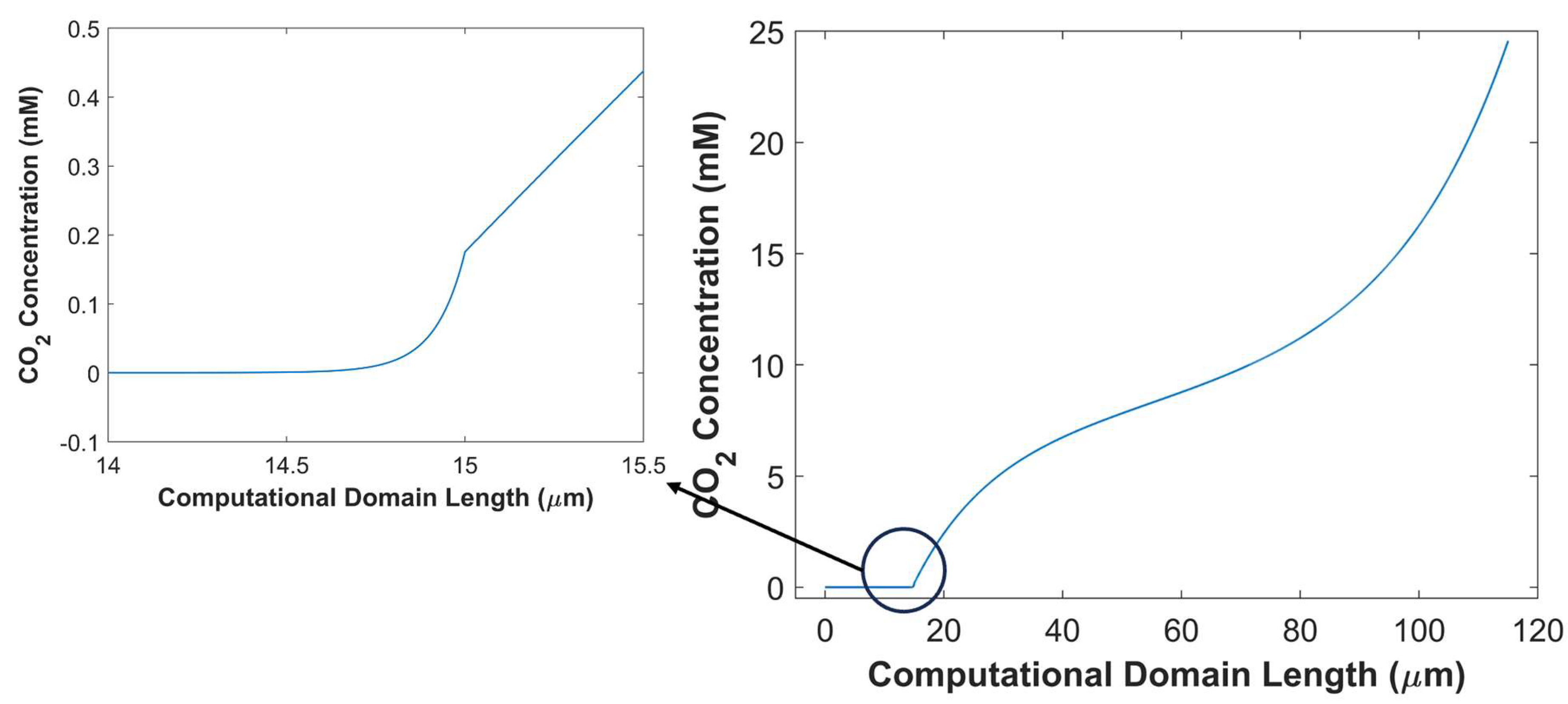
Figure 14.
Effect of 1 M KOH and 1 M KHCO3 electrolyte on TCD.
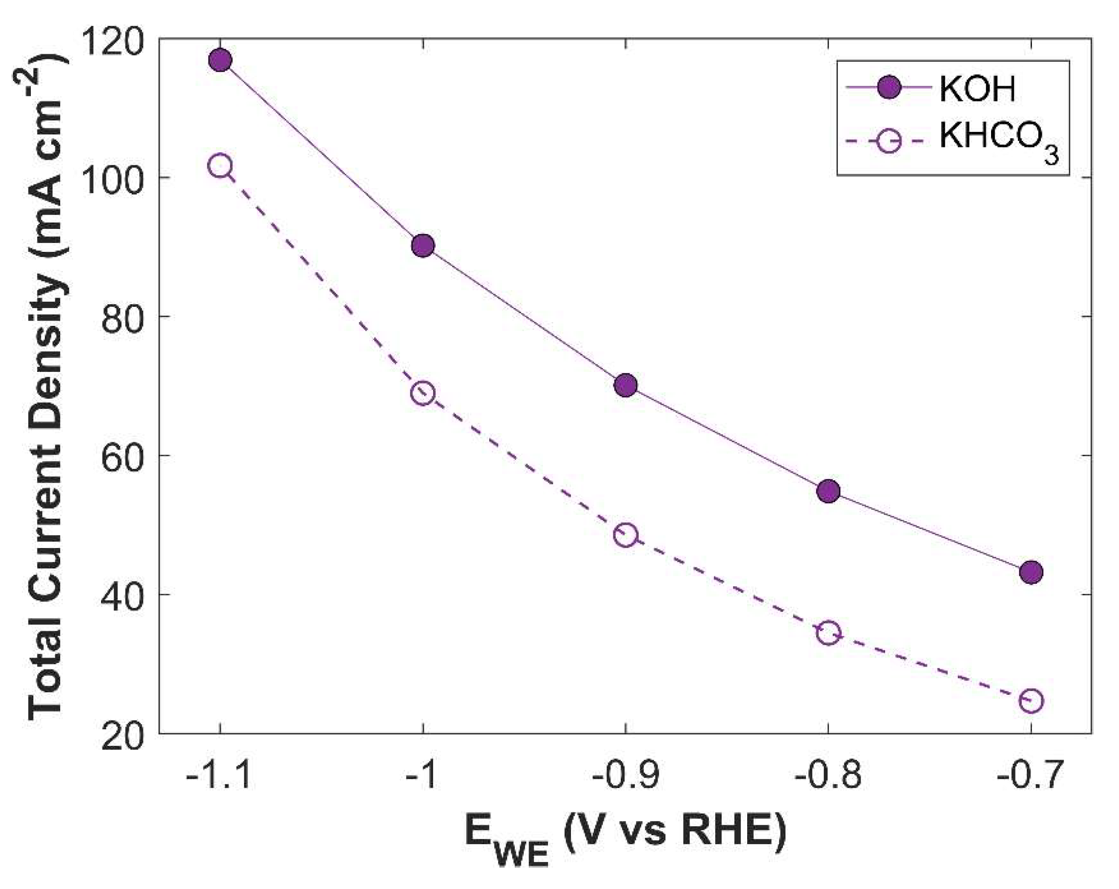
Figure 15.
Average surface CO2 concentration when using 1 M KOH and 1 M KHCO3 as an electrolyte.
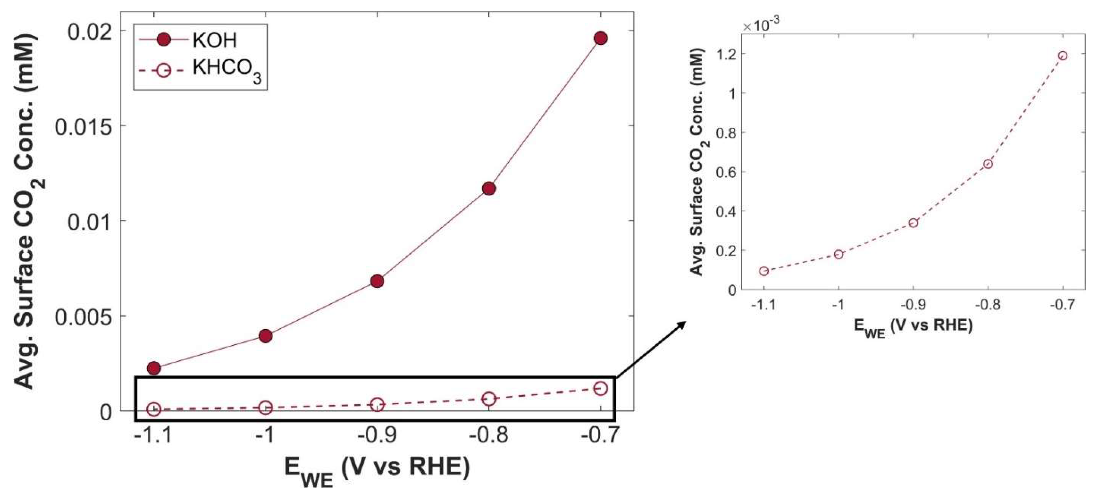
Figure 16.
PCD of CO2 reduction products using 1 M KHCO3 electrolyte.
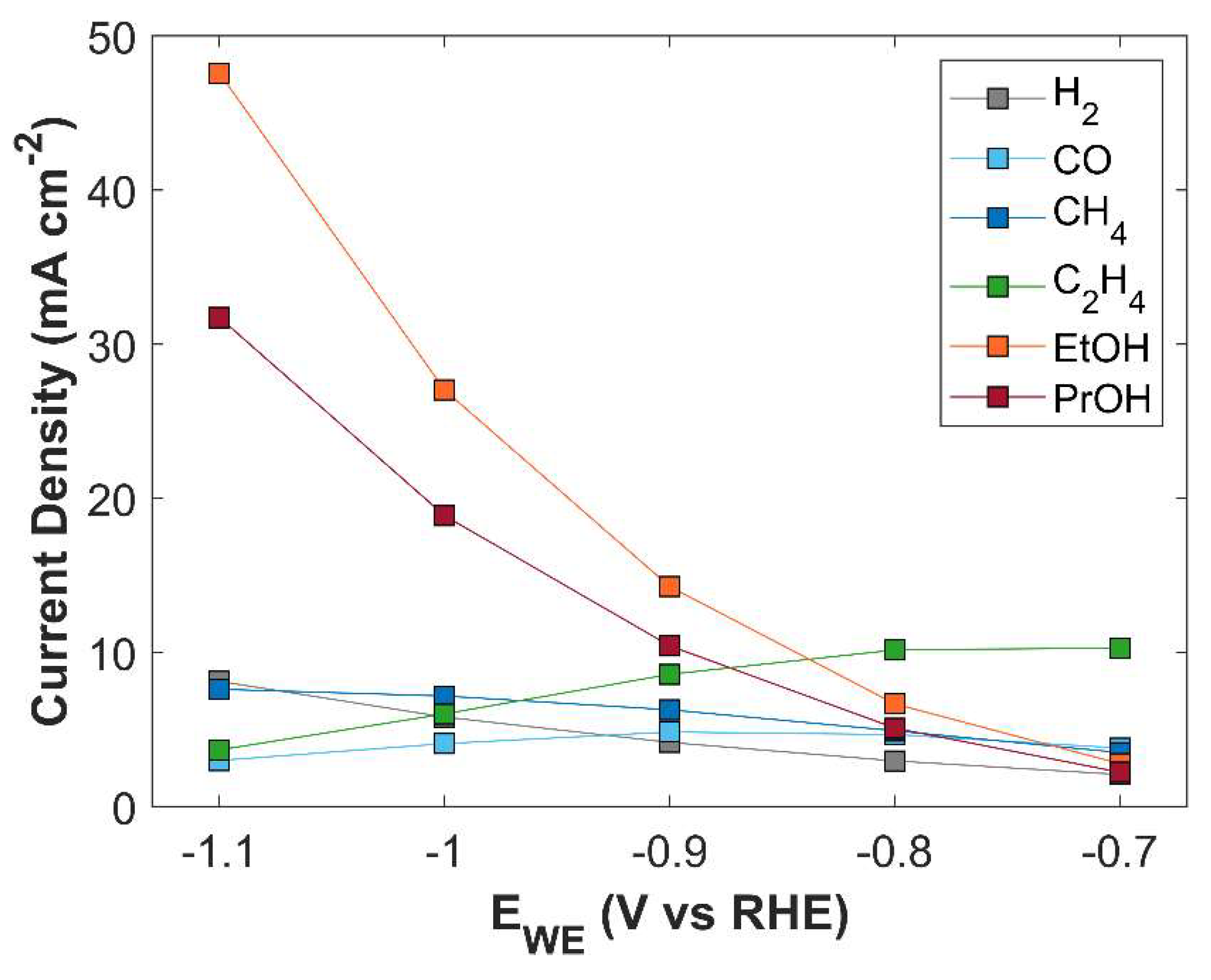
Figure 17.
Effect of electrolyte strength on TCD. Applied cathodic potential is -1.0 V vs RHE.
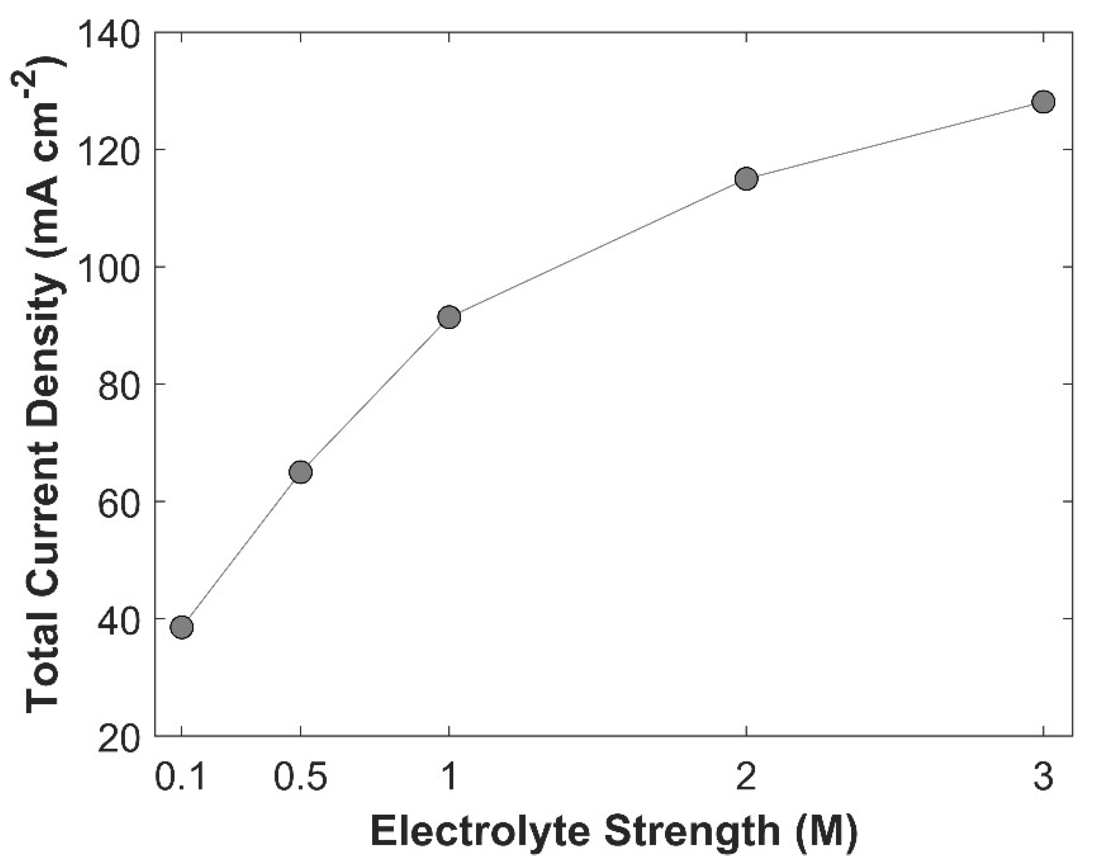
Figure 18.
Average surface concentration of CO2 as a function of electrolyte strength at a fixed applied potential of -1.0 V vs RHE.
Figure 18.
Average surface concentration of CO2 as a function of electrolyte strength at a fixed applied potential of -1.0 V vs RHE.
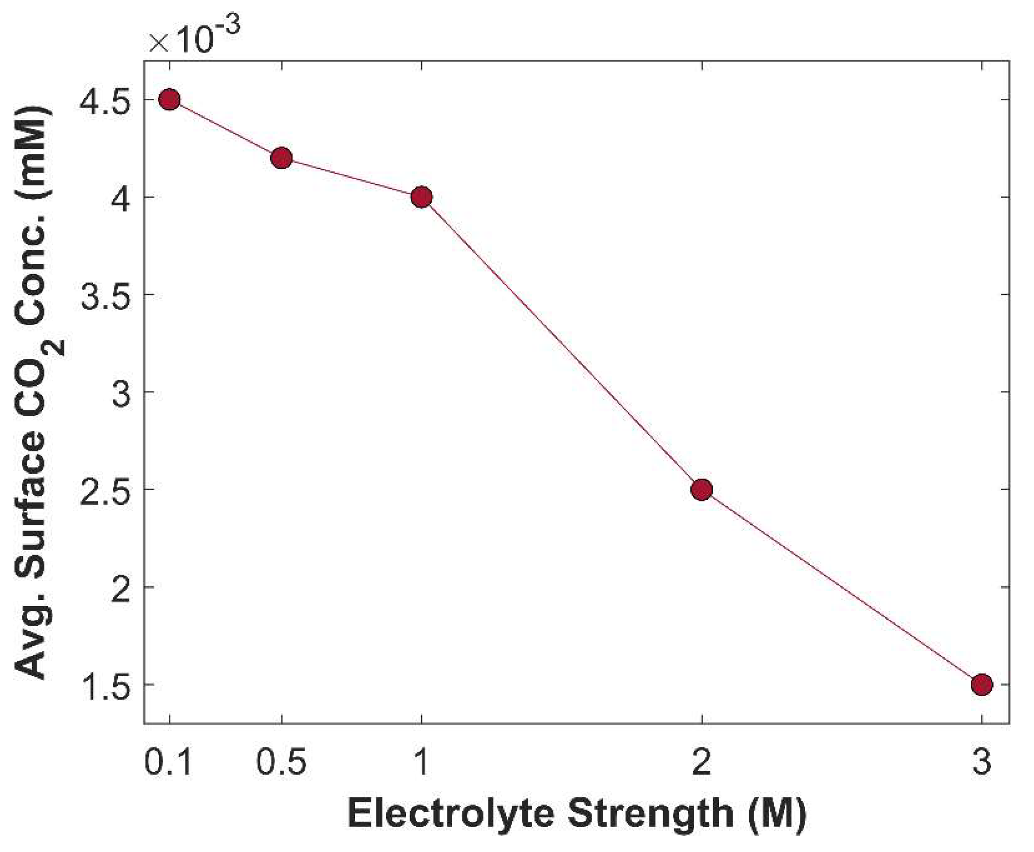
Figure 19.
TCD comparison of 3 different electrode configurations: SE, GDLE, and GCE.
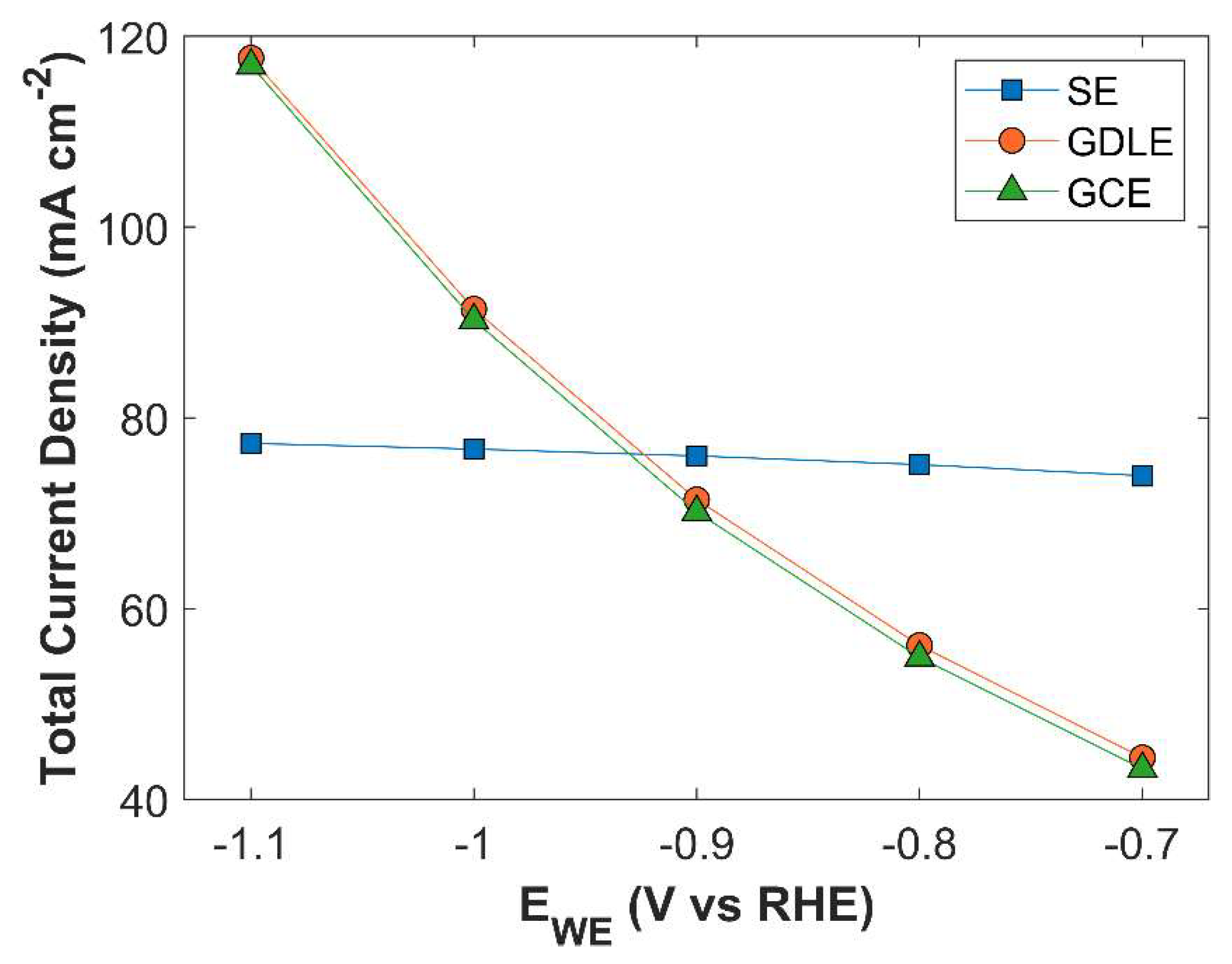
Figure 20.
Average surface CO2 concentration as a function of applied cathodic potential for three different electrode configurations.
Figure 20.
Average surface CO2 concentration as a function of applied cathodic potential for three different electrode configurations.
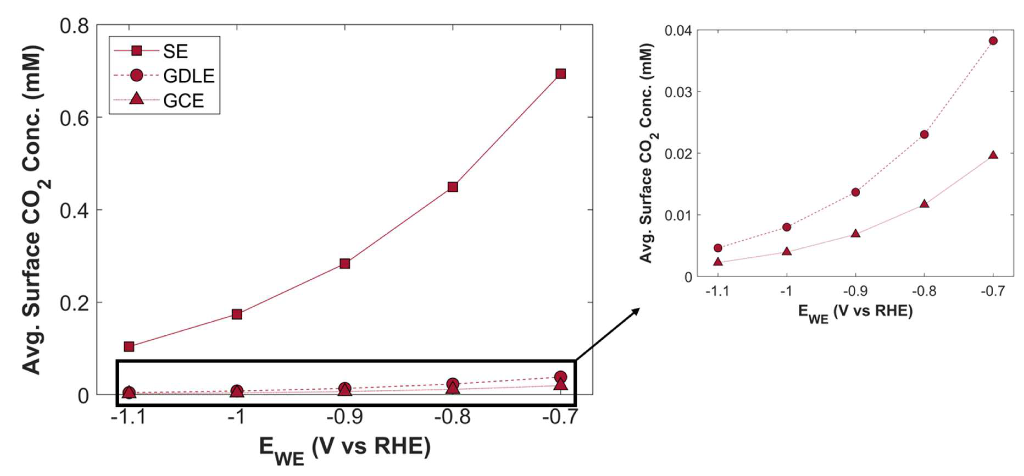
Table 1.
Electrochemical CO2 reduction reactions for CuAg0.5Ce0.2 catalyst.
| Species | Reactions |
|---|---|
| H2: | |
| CO: | |
| CH4: | |
| C2H4: | |
| EtOH: | |
| PrOH: |
Table 2.
Chemical reaction of CO2 with electrolyte in alkaline media.
| R1: | K1 (1/M) | |
| R2: | K2 (1/M) | |
| Rw: | Kw (M2) |
Table 3.
List of Sechenov’s constants [50].
Table 3.
List of Sechenov’s constants [50].
| Constants | Values |
|---|---|
| -0.0172 | |
| -0.000338 | |
| 0.0922 | |
| 0.0839 | |
| 0.0967 | |
| 0.1423 |
Table 5.
Pre-simulation estimates for local CO2 concentration, and pH values using experimental data of CuAg0.5Ce0.2 catalyst.
Table 5.
Pre-simulation estimates for local CO2 concentration, and pH values using experimental data of CuAg0.5Ce0.2 catalyst.
| TCD | CO2 | pH |
|---|---|---|
| (mA cm-2) | (mM) | |
| -47 | 15.747 | 11.072 |
| -64 | 12.150 | 11.128 |
| -84 | 8.0113 | 11.219 |
| -105 | 6.1246 | 11.28 |
| -131 | 4.2034 | 11.368 |
Table 6.
Batch-cell model parameters.
| Parameter | Value | Unit | Reference | |||
|---|---|---|---|---|---|---|
| Design Parameters | ||||||
| LCL | 15 | Experimental input | ||||
| LBL | 100 | Fitted | ||||
| LGDL | 325 | Experimental input | ||||
| T | 298 | K | This study | |||
| EWE | -0.7 – -1.1 | V vs RHE | ||||
| Electrochemical Kinetic Rate Parameters for CuAg0.5Ce0.2 Catalyst | ||||||
| 97.3 | mA cm-2 | This Study | ||||
| 8.89 x 10⁸ | mA cm-2 | |||||
| 9.50 x 10⁵ | mA cm-2 | |||||
| 2.8 | mA cm-2 | |||||
| 4.10 x 10⁻² | mA cm-2 | |||||
| 9.50 x 10⁻³ | mA cm-2 | |||||
| 0.0274 | ||||||
| 0.1001 | ||||||
| 0.1391 | ||||||
| 0.1222 | ||||||
| 0.1490 | ||||||
| 0.1676 | ||||||
| 0 | V vs RHE | [38] | ||||
| -0.11 | V vs RHE | |||||
| 0.17 | V vs RHE | |||||
| 0.07 | V vs RHE | |||||
| 0.08 | V vs RHE | |||||
| 0.09 | V vs RHE | |||||
| Chemical Reaction Rate Parameters | ||||||
| 5.93 x 10⁻³ | m3 mol-1s-1 | [27] | ||||
| 1.0 x 10⁻⁸ | m3 mol-1s-1 | [27] | ||||
| 0.04 | s-1 | [24] | ||||
| 56.281 | s-1 | [24] | ||||
| 0.001 | mol L-1s-1 | [26] | ||||
| 1.34 x 10⁻⁴ | s-1 | [27] | ||||
| 2.15 x 10⁻⁴ | s-1 | [27] | ||||
| 9.37 x 10⁴ | L mol-1s-1 | [24] | ||||
| 1.23 x 10¹² | L mol-1s-1 | [24] | ||||
| 1.0 x 10¹¹ | L mol-1s-1 | [26] | ||||
| Porous Media Properties | ||||||
| 0.72 | This Study | |||||
| 0.3 | This Study | |||||
| 220 | S m-1 | [24] | ||||
| 100 | S m-1 | [24] | ||||
| 1.0 x 10⁷ | m-1 | This Study | ||||
| Liquid Species Diffusion Coefficients | ||||||
| m2 s-1 | [51] | |||||
| m2 s-1 | [51] | |||||
| m2 s-1 | [52] | |||||
| m2 s-1 | [52] | |||||
| m2 s-1 | [53] | |||||
| m2 s-1 | [53] | |||||
Table 7.
Additional reversible chemical reactions.
| R3: | K3 (M) | |
| R4: | K4 (M) |
Disclaimer/Publisher’s Note: The statements, opinions and data contained in all publications are solely those of the individual author(s) and contributor(s) and not of MDPI and/or the editor(s). MDPI and/or the editor(s) disclaim responsibility for any injury to people or property resulting from any ideas, methods, instructions or products referred to in the content. |
© 2025 by the authors. Licensee MDPI, Basel, Switzerland. This article is an open access article distributed under the terms and conditions of the Creative Commons Attribution (CC BY) license (http://creativecommons.org/licenses/by/4.0/).
Copyright: This open access article is published under a Creative Commons CC BY 4.0 license, which permit the free download, distribution, and reuse, provided that the author and preprint are cited in any reuse.


