
Submitted:
29 November 2024
Posted:
02 December 2024
You are already at the latest version
Abstract
This paper provides an integrated overview of the three-year effort to design and implement a prototypical SAA system based on a multisensory architecture leveraging data fusion between optical and radar sensors. The work was carried out within the context of the Italian research project named TERSA (Electrical and radar technologies for remotely piloted aircraft systems) undertaken by the University of Pisa in collaboration with its industrial partners, aimed at the design and development of a series of innovative technologies for remotely piloted aircraft systems of small scale (MTOW < 25 Kgf). The approach leverages advanced computer vision algorithms and an Extended Kalman Filter to enhance obstacle detection and tracking capabilities. The “Sense” module processes environmental data through a radar and an electro-optical sensor, while the “Avoid” module utilizes efficient geometric algorithms for collision prediction and evasive manoeuvre computation. Initially, this integrated system has been rigorously tested by means of a sophisticated simulation environment that replicates real-world conditions, including the generation of realistic artificial scenery to evaluate the closed loop interaction between sense and avoid modules in a Hardware-in-the-Loop (HIL) setup. Preliminary results demonstrate the system’s effectiveness in real-time detection and avoidance of non-cooperative obstacles, providing high computational efficiency and responsiveness while ensuring compliance of UAV aero mechanical constraints and safety constraints in terms of minimum distance requirements. At a later stage of the project, the effectiveness of the integrated system was evaluated by means of a preliminary flight test campaign conducted at the Lucca-Tassignano airport in Italy. The findings underscore the potential for deploying such advanced SAA systems in tactical UAV operations, contributing significantly to the safety of flight in non-segregated airspaces.
Keywords:
Sense and Avoid
; Object detection and Tracking
; Unmanned Aerial Vehicles
; Data fusion
; Collision Avoidance
1. Introduction
During the recent years, Unmanned Aircraft Systems (UAS) and their operations have registered a significant increase in number, sophistication and technical complexity. UAS are no longer a military exclusive reality, but several studies are currently evaluating their possible employment in a broad variety of civil applications. These range from monitoring and surveillance tasks such as border and maritime patrol mission, search and rescue operations, forest fire detection, road traffic surveillance, critical infrastructure protection to commercial purposes such as aerial imagery, crop assessment in agriculture and communication relays [1,2,3]. This rapid expansion is motivated by the unmatched versatility in terms of application scenarios that these systems offer, both military and civil, and by the numerous advantages connected with the employment of a vehicle that doesn’t require a pilot onboard. However, the lack of the presence of a human pilot onboard, also poses a series of safety related concerns and technical challenges mainly connected with the risk of a mid-air collision with another aircraft, that may hinder the successful integration of unmanned aircraft in civil non-segregated airspace [4]. For instance, in Italy, UAV operation is restricted within Visual Line of Sight (VLOS) by the Italian regulatory authority (ENAC) and a specific request must be filed and approved every time a Beyond Visual Line of Sight (BVLOS) operation is to be conducted [5]. Moreover, in the past years, Aeronautical agencies and authorities were involved in the definition of proper regulations to allow UAVs for a safe access to flight, culminating with FAA issuing mandatory installation, onboard UAVs, of dedicated systems for autonomous obstacle detection and avoidance, as a requirement for non-segregated flight operation [6]. Such systems are required to meet or exceed human capabilities in terms of avoiding potential collision threats, a concept that several authors [7,8] refer as “equivalent level of safety” that the UAS should possess for the safe integration in the global airspace. Consequently, a huge effort by worldwide research institutions has been put into place to devise proper Sense and Avoid (SAA) systems with the overall goal of mitigating the risk of mid-air collision between UAVs and other aircraft. The limitations connected with UAS own size and weight, the so-called SWaP (Seize, Weight and Power constraints), severely impact the implementation of autonomous collision avoidance solutions often preventing the adoption of more consolidated technologies such as TCAS [9] or ADB-S. Such constraints often impose to solve real-time, complex, detection and tracking problems utilizing the limited computational resources available onboard. In addition, the fundamental requirement of being able to autonomously detect and avoid non-cooperative intruders which are generally not equipped with transponders and do not take active part in the conflict resolution, force the designer to develop innovative solution leveraging a multitude of sensors with the aim of rendering UAS capable of solving the impending conflict on its own. From a taxonomical standpoint, SAA systems are usually categorized according to the sensor type they rely on, which can be active or passive. For the former case, radar exploiting Frequency Modulated Continuous Wave (FMCW) technology is becoming more and more popular for SAA purposes because of the economical, low Size, weight and power solution they offer. Besides, radar sensors appear interesting because they provide positioning information (in terms of range, range rate and angular measurement) practically under any weather or illumination condition. Several works have investigated the use of radar sensors for SAA applications: in [10] a SAA system comprising the combination of cooperative sensors (TCAS and ADB-S) and a radar is tested in an extensive flight trials campaign; the authors in [11] describe an algorithm for safe navigation of small-sized UAVs within an airspace leveraging secondary Surveillance Radar (SSR); other examples of UAV detection methods based on radar are described in [12,13]. Radar is not the only active sensor which is being investigated for SAA applications. An example of another active sensor, the LIDAR, currently studied for SAA applications is provided in [14]. Passive sensors and specifically optical sensor, on the other hand, generally offer a higher accuracy in terms of target angular position reconstruction, a higher refresh rate and a lower power absorption and weight; their main drawbacks lies in the fact that their operation is severely limited in low lighting conditions (i.e. night) and direct target position reconstruction is not possible because a single camera sensor can’t measure distance directly. In [15] the problem of estimating target distance with only a camera sensor is overcome by means of a depth estimation model based on a lightweight encoder-decoder architecture trained on a large database of airborne object. The deep learning model is trained to translate the input image from the monocular camera to a depth mask, classifying every pixel into depth values. In [16] the authors leverage an implementation of the You Only Look Once (YOLO) object detector to detect cooperative micro UAV within the FOV of a camera. Sensor data coming from the cooperative navigation system are exploited to reduce the search window in a strip of the image which is computed starting from the approximate relative position of the two UAVs and attitude information of the UAV where the camera is mounted. Other examples of different strategies employed to tackle the task of intruder detection relying solely on camera sensor can be found in [17,18]. Other authors have instead favoured an approach exploiting the fusion of passive and active sensors. This choice is motivated by the fact that sensor fusion strategies can leverage the complementary advantages of different sensor sources. For example, in [19] a radar/visual fusion approach designed to fuse the radar and visual tracks is discussed for a non-cooperative Sense and Avoid system for low altitude flying UAVs. In [20] an integrated Sense and Avoid system developed by the Italian Aerospace Research Centre (CIRA) and the university of Naples and deployed onboard a customized TECNAM P-92, based on data fusion between EO and radar sensor is thoroughly discussed. In the work, particular focus is placed on integration details, fusion logics, algorithms and flight results relevant to the achievable situational awareness. A radar/visual multisensory architecture was chosen also for the implementation of one of the activities of the recently concluded Italian project named TERSA. The project aimed at the design and development of several innovative technologies for a lightweight UAV including the development of a collision avoidance system for unmanned aerial vehicles leveraging data fusion between optical and radar sensor. The project involved the University of Pisa (UNIPI) and a consortium of industrial partners led by the Italian UAV manufacturing company Sky Eye Systems (SES), and it led to the development of a fully autonomous SAA system to be installed onboard a new generation of lightweight UAV manufactured by SES in Italy. This work presents an overview of the system that was developed during the project, from the identification and definition of the technical requirements to the actual flight test conducted to validate the system. Specifically, the present article is organized as follows: the reminder of this first Chapter describes the high level requirements of the system; Chapter II briefly recalls the sense and avoid system architecture developed during the project; Chapter III details the principal algorithms designed for the implementation of the system, with particular focus to the computer vision object detection and tracking algorithms and the data fusion strategy adopted; Chapter IV describes the numerical simulations conducted to validate the system providing an overview of the integrated HIL simulation environment that was developed at the Fly-By-Wire laboratories of the Civil and Industrial Engineering Department of the University of Pisa; Chapter V describes the flight test campaign conducted in cooperation with Sky Eye System (SES), and ECHOES radar technologies, the partner who manufactured the radar, aimed at the validation of the integrated system. Finally, Chapter VI presents the conclusion of the research work and provides an outlook of the future developments.
1.1. Reference Aircraft
1.2. System High Level Requirements
UAV autonomous anti-collision systems are still at a developing stage and research studies are still being carried out to identify system requirements and sensing solutions. As a consequence, at present, specific requirements to be met by the system designer don’t exist; however, a collection of universally accepted specifications, guidelines and recommendations formulated by ICAO [21,22], FAA [8], ASTM [23], EUROCONTROL [24], RTCA [25] and other researcher [26,27] has been used to define the system requirement for the present application. A SAA system is usually composed of two main modules. The sense module, from a functional standpoint must acquire information from the environment to contribute building awareness of what is happening in the vicinity of the UAV and to detect potential hazards. The task of the avoid module, on the other hand, is to guarantee both a separation-provision and a collision-avoidance function. By separation provision is intended the capability to separate the UAVs from other aircraft whenever Air Traffic Control (ATC) is not providing separation. The Pilot in Command (PIC) should be warned by the system following a loss of separation so that PIC may manoeuvre as required. System should immediately prompt the PIC as soon as separation is restored and should seek for approval to return on initial trajectory. This function should separate the UAV from other aircraft by a minimum distance of 0.5 NM in the horizontal plane and 500 ft in the vertical plane. Collision-avoidance function instead should operate independently from ATC and should either provide the PIC with valuable cues about an impending collision, waiting for him to employ corrective actions or should autonomously resolve imminent collision executing avoidance manoeuvres. Several requirements can be pointed out both for sense and avoid modules.
1.2.1. Sense Requirements
Principal requirements are summarized below:
- Detection range, It is connected to the time-to-collision by means of approaching speed. It must be sufficiently large to allow for an avoidance manoeuvre complying with aircraft dynamic, structural and aerodynamical constraints that guarantees a minimum separation of 500 ft at the closest point of approach to the obstacle (“miss distance”) [23]. For the characterization of this requirement, the procedure described in [27] has been adopted by considering the most critical condition of a frontal encounter. Since the evasive manoeuvre will be conducted by means of a corrected turn on the horizontal plane, essentially depends on four factors: UAV speed, intruder aircraft speed, latency between detection and evasive command execution and especially the minimum turn radius. As well known, minimum turn radius (in stationary manoeuvre at constant altitude and speed) for a conventional fixed wing aircraft depends on three constraints: aerodynamic, structural and propulsive. As an example, Figure 2 (a) shows the minimum attainable turn radius at sea level for the TERSA aircraft according to each constraint where realistic bounds have been assumed for maximum lift coefficient , maximum vertical load factor , and available thurst (actual exact values provided by the manufacturer have been omitted due to NDA reasons). A lower threshold of is enforced by the FCS as a stall protection mechanism. As it can be noted, in the range of operative flight speeds (), structural constraint is the only effective bound but in turn is capped by the stall protection limit. Figure 2 (b) shows the required minimum detection range for various intruder speed and UAV minimum turn radius, according to the procedure described in [27] (conservative estimate with a delay factor of between detection and evasive command execution). A detection range of appears satisfactory for the effectiveness of a collision avoidance maneuver with an intruder flying at a comparable cruise speed as the UAV.
- Field of View: A widely accepted guideline for manned aircraft manufacturers is to build cockpits as to ensure a visibility of ±110° (azimuthal) and ±15° (in elevation) [23]. Usually, the same requirement is extended to Unmanned aircraft. However, due to the prototypical nature of this system a FOV of ±60° has been identified as the design requirement. As a matter of fact, preliminary sensitivity analysis conducted on a wide range of collision encounter scenarios, considering an intruder cruise speed comparable with the UAV cruise speed, have shown that, given an assigned detection range , FOV anlges greater than 55° don’t substantially affect the detectability of the intruder aircraft.
- Refresh rates: For a precise tracking of the intruder aircraft, computer vision algorithms should run at a sufficiently high frequency (> 10 FPS). Given the limited computational power available on board, it is thus essential to optimize object detection and tracking algorithms and to select the best compromise between image resolution and performance. Data fusion algorithms are based on a standard implementation of an extended Kalman filter and thanks to optimized linear algebra libraries do not pose a significant computation burden on the VPU processor. Likewise, collision avoidance routines, that exploit simple geometric laws, do not constitute a bottleneck for performance; the computation of the setpoint on the desired ground track angle to carry out the maneuver, essentially boils down to the extraction of the roots of a 4th order polynomial which again is performed effectively on the VPU processor by means of optimized linear algebra libraries (OpenBLAS/cuBLAS). The bottleneck is thus represented by the object detector pipeline.
- Optical sensor resolution: the choice of the optimal compromise is the result of a trade-off between computational efficiency and capability of detecting small targets at a great distance. The performance of the visual tracker chosen for the implementation of the system is essentially independent of the resolution because it acts on a finite set of discrete anchor points. On the contrary, the object detection pipeline is strongly affected by the size of the image as detailed in chapter 3. At the same time, a higher resolution is beneficial for two major reasons:
- The attainable maximum angular resolution can be expressed as:where is the horizontal pixel density of the sensor and the focal length.
- Johnson criteria states that the maximum distance at which an object of physical characteristic size of can be detected by an optical sensor, denoting with the minimum number of pixel the object needs to occupy for a successful detection (Johnson’s factor usually assumed = 2) and with the physical size of the pixel, is given by [27]:
For a given sensor’s size, the higher the resolution, the lower the single pixel physical size. For these two reasons, it is thus clear that a higher resolution would be beneficial. For the development of the system, considering the specifics of the Vision Processing Unit chosen (see Chapter 2) and the typical dimensions of the UAVs belonging to the same class as the TERSA aircraft, a resolution of was chosen.
1.2.2. Avoid Requirements
Given the prototypical nature of the system, some simplified assumptions have been made during the definition of the requirements for the collision avoidance module that can be summarized as follows:
- One single intruder aircraft present at a given time in the conflict scenario belonging to the same UAV class with comparable cruise speed and altitude.
- Such aircraft maintains its original linear stationary flight course, wing levelled, constant speed. Several combinations of relative initial positions and relative speeds are evaluated.
- Evasive maneuver is conducted by means of a correct turn on the horizontal plane, conducted at constant speed and altitude.
The reason for a climbing evasive maneuver has not been considered is briefly justified in the following. A study has been conducted evaluating the maximum flight path angle attainable by the reference aircraft in a steep (stationary) climb maneuver utilizing aero mechanical dataset provided by courtesy of SES. Specifically, as well known, the maximum attainable flight path angle is given by:
where is the available thrust, is the aerodynamic drag and the aircraft weight. Considering the equilibrium in the vertical plane:
And applying the principle of superimposition of effects (PSE), former equations can be expressed by means of Eq. (5) where the terms represent variation w.r.t to the reference condition.
Once the trim problem is solved for AOA and elevator deflection ensuring equilibrium, ( respectively), drag force is computed by means of Eq. (6)
Available thrust as a function of flight speed, engine RPM and altitude is obtained by means of engine maps provided by courtesy of SES. Figure 3 shows the attainable as a function of RPM and flight speed at a given altitude.
The exact value of for a given altitude is found by solving the maximization of the expression (3) while enforcing the respect of trim equilibrium described by (5). For instance, at an altitude of 9.57° corresponding to a True air speed of TAS = 18.8 and an engine setting of 7950 RPM. Considering a detection range of , this would result in a , insufficient to ensure a minimum separation provision of as recommended in the guidelines. It should be noted that the actual minimum separation attainable with a climbing manoeuvre alone would be even smaller than the afore mentioned estimate due to engine and aircraft dynamics which prevent the onset of an immediate maximum flight path angle and unavoidable latencies between actual detection and evasive command implementation.
Granted that a climbing manoeuvre alone wouldn’t provide necessary separation to avoid the obstacle and given the prototypical nature of the application, it is decided to carry out the evasive action by means of a coordinated turn on the horizontal plane.
The requirements of the avoid modules are thus hereby summarized:
- Once a threat has been positively identified by the sense module, the avoid function has to perform an avoidance manoeuvre in a completely autonomous fashion which guarantees minimum separation provision at all times between the UAV and the intruder aircraft. The Autonomous Collision Avoidance (ACA) strategy employed must be effective for non-cooperative intruders.
- Such manoeuvre must be conducted on the horizontal plane by means of a coordinate turn that takes into account the aerodynamic and structural limits of the UAV.
- After the conflict has been deemed resolved by the Conflict Detection and Resolution (CDR) algorithms, the avoid module must bring the UAV on his original trajectory.
- It is desirable that the avoidance manoeuvre produces the minimum deviation from the original planned trajectory of the UAV.
2. System Architecture
The Typical integration of a SAA system within the closed loop control system of an UAV is shown in Figure 4. As can be noted, the underlying algorithms take as input the UAV position and velocity states provided by the Inertial Navigation System (INS) and the velocity and position states of the intruder aircraft and yield as output, in the most general case, the demanded speed, flight path angle and ground track angle which in turn are fed as input to the autopilot system to avoid the collision threat.
For this specific application, the only output of the SAA system is the demanded heading angle used as setpoint for the coordinated turn on the horizontal plane. For the actual implementation of the system, a multisensory architecture leveraging data fusion between radar and EO sensor has been chosen. As it has been shown in several previous works [20,27,28] this allows to compensate for the shortcomings of each sensor type, reduce noise and increase the overall solution accuracy. In particular, data fusion between radar and EO sensors leads to an increase in system robustness with respect to false alarms and missed detections during the object detection stage, coupled with a higher accuracy in the tracking stage. A diagram portraying the high-level schematics of the developed architecture is shown in Figure 5. The working principle of the system can be summarized as follows: both the EO (camera) sensor and the radar scan the environment ahead of the UAV in search of a potential threat. Each new frame captured by the camera is compared against a background model of the scene leveraging an object detection strategy based on Single Gaussian Model (SGM), where suitable motion compensation algorithms are employed to compensate for the ego motion of the camera.
A Ransac approach is used to derive the homography matrix describing the transformation between current frame and background model, starting from point correspondences between the two scenes. Background model is then warped according to this transformation as to co-register it to the current frame and minimize the noise due to camera ego-motion. Connected component analysis (CAA) is then used to group various blobs in the binary mask into a single object of interest. Statistical criteria are then applied to validate only those tracks that exhibit a certain regularity in terms of position within the field of view and dimensions across the various frames; more details on the specific algorithms involved are provided in the subsequent chapters. A validated track is then followed across various frames leveraging an implementation of the Kanade Lucas Tomasi (KLT) feature tracker [29]. From the knowledge of camera parameters (focal length, resolution and sensor size) track centroid position in terms of pixel within the scene is then transformed into relative elevation and azimuth angles, as shown in Figure 6 by means of Eq. (7). Here, are the azimuth and elevation angles respectively in a reference system fixed with the camera, are the sensor width and height respectively, the vertical and horizontal resolution of the scene, the focal length and the vertical and horizontal position of the intruder aircraft within the scene (expressed in pixel).
The knowledge of the target distance provided by the radar allows to close the tracking problem. Specifically, distance measure, elevation and azimuth angles together with UAV position, velocity and attitude states are fed as input to an Extended Kalman Filter (EKF) which carries out data fusion and outputs intruder aircraft velocity and position states expressed in an inertial reference system. These states are then fed as input to collision avoidance routines which compute an evasive manoeuvre when an impending collision is predicted. A new setpoint on the heading angle is computed at every iteration step in a such a way that the trajectory of the UAV will be tangent to a sphere centred around the intruder aircraft in the point of closest approach. More details about the designed algorithms are provided in chapter 3.
System Components
The main components identified for the realization of the system are:
- A range doppler radar in Ku-band (13.325 GHz) with forward-looking configuration. Radar emits a Linear Frequency Modulated Continuous Wave (FMCW) with a maximum transmitted band of 150 MHz. Azimuth estimation is obtained by means of monopulse amplitude technique.
- Electro-optical sensor with at least 30 FPS, HD ready resolution. Focal length must be chosen to ensure a sufficiently high FOV.
- Vision processing Unit. An embedded platform with low power absorption, easily interfaceable with camera and radar (through ethernet) must be chosen, ideally optimized for computer vision tasks. Both Sense and avoid algorithms run on the embedded platform
- An Inertial Measurement Unit (IMU) must be employed to retrieve attitude angles which are necessary to transform intruder aircraft position and velocity states into the inertial frame where the conflict is resolved.
3. Algorithms Design
The present section details the implementation of principal algorithms underlying the sense and avoid system.
3.1. Sense Module
As explained above, for the implementation of the system, a multisensory architecture based on data fusion between electro-optical (EO) and radar sensor was chosen. Digital Image processing algorithms thus play a crucial role for the correct functioning of the SAA system. The three main tasks such algorithms are called to perform can be summarized as:
- 4.
- Segmentation between background and objects of interest within the FOV with the aim of identifying the presence of an intruder aircraft, Object Detection (OB).
- 5.
- Carry out noise suppression due to camera ego-motion, Ego Motion Compensation (EMO)
- 6.
- Once the presence of an object has been confirmed, track its motion efficiently across frames after its identification.
The requirement of achieving a sufficiently high frame rate on the VPU chosen, to allow for an effective target tracking while at the same time maintaining a sufficiently high precision to distinguish small targets at a great distance from the optical sensor, guided the entire designing process.
Figure 7 shows a high-level schematic of the adopted computer vision pipeline underlying the sense module. Some of the key algorithms constituting the building blocks of the pipeline (such has Harris Corner detector and Kanade Lucas Tomasi feature tracker) appear at several stages of the processing chain; they will be briefly explained in the following.
3.1.1. Harris Corner Detector
The Harris Corner Detector [30] is one of the most well-known, robust and efficient algorithms for extracting singular points within a digital image. Singular points are points of considerable importance as they tend to be invariant to translation, rotation and changes in illumination; their stability makes them ideal for, among other, image tracking or stabilization applications. The name corner derives from the fact that they are usually located at the intersection of at least two edges within the image, where an edge is defined as an area characterized by a sudden, sharp change in light intensity. Consider a digital image of size and a small window of size ; then a shift of the window in a certain direction will either produce negligible change in mean intensity, if the window lies above a flat region, a substantial change in mean intensity value when shifting in two orthogonal direction if the window lies over a corner and lastly if the window lies over an edge, the shift will produce a substantial change while shifting along a direction but a negligible one if shifting along the orthogonal direction. Mathematically, this can be expressed in terms of the Sum of Square Differences (SSD) of the intensity values of all the pixels within the window before and after the translation as:
where is a weight matrix, denotes the intensity value of the pixel located at position and denotes the intensity value of the same pixel after a small shift of the window in the direction .
By means of Taylor expansion, Eq. (8) can be rearranged as:
where the matrix is generally referred as the structural tensor with representing (spatial) horizontal and vertical image gradient respectively. Eigenvectors of M matrix denote the directions along which the mean square deviation takes on maximum and minimum values. When both the associated eigenvalues are sufficiently high (in a relative sense with respect to the others), the patch is above a singular value (corner point). A suitable Harris response, defined as:
Is used in place of the actual eigenvalues computation, where The chosen implementation is articulated in the following steps:
- Gray scale conversion of original image
- Spatial gradient calculation by means of linear spatial convolution with kernels and its transpose
- Structural tensor calculation for each pixel in a window centered around the pixel.
- Harris response calculation, by computing trace and determinant of M matrix.
- Non maxima suppression (to eliminate duplicate points) and thresholding: in a nutshell, only those points whose response is higher then 1% of the maximum R are selected as valid points.
- Biquadratic fitting to refine corner position and obtain a subpixel location.
3.1.2. Kanade Lucas Tomasi Feature Tracker
The KLT feature tracker is a well-known, efficient feature tracking algorithm which exhibits some robustness w.r.t the change in illumination condition, camera motion, and change of appearance of the tracked object. In its pyramidal implementation [31], it is capable of tracking large motions while preserving a small integration window. The algorithm finds correspondences of points from a primary image and a secondary image by solving a non-linear optimization problem. It attempts to minimize the residual function defined as:
where is the displacement vector to be determined, is the current corner point under evaluation and is an integration window centered on it. The objective of the algorithm is to find the position of a corresponding window centered on the pixel on the secondary image, such that the sum of square differences among the intensity values is minimized. The vector is called optical flow and is the unknown to be determined. Applying Taylor expansion to Eq. (11) and setting its derivative with respect to displacement to zero (at the optimum there should be no change in intensities values) yields:
where the quantity can be interpreted as the time derivative of the intensity values of the image in the point , whereas the matrix is simply the spatial gradient of the intensity values of the secondary image (current frame). For a purely translational displacement, it can be proved that intensity gradients of the primary and secondary images are interchangeable i.e.
This fact is exploited in the implementation leading to great computational advantage because for each image, for each pyramidal level, gradients are computed only once. Gradients are computed by means of the central difference operator Eq. (14)-(15)
Plugging equations (14)-(15) in (12) yields Eq (16).
Now, defining the so-called image mismatch vector as:
And the structural tensor as:
Eq. (16) can be rewritten as:
Which yields the optical flow solution:
Notice that in chosen implementation, the matrix G is constant for each pyramidal level, thus the computation of image gradients (an expensive operation that involves spatial convolution) is performed only once per pyramidal level; the only quantity updated at each iteration is the image mismatch vector which is a function of the difference between the reference window centered around the current pixel in the primary image (which is constant) and window in the secondary image which is a warping of the original window. Notice however that the interpolation required to compute the warped window is not performed on the entire image but only on the window, thus the smaller the window the faster the algorithm. Since the maximum displacement that can be tracked is equal to half the window size, the pyramidal implementation is a clever approach to track higher displacement while preserving a small window and thus computational efficiency. Essentially, each pyramid level is a down sampled version of the original image with a subsample factor of 2. When the algorithm converges at a the level, the displacement is propagated at the level and used as a new starting point. A visual representation of the pyramidal expansion is shown in Figure 8. An example of matched points correspondences for an aeronautical sequence is shown in Figure 9. Finally, a high-level scheme of the implemented algorithm is provided in Figure 10.
3.1.3. Object Detection
Several approaches exist in literature to address the problem of detecting an object of interest within the FOV. These algorithms range from simple colour thresholding, to edge detection coupled with proper thresholding and morphological operations [32], segmentation based on motion estimation through optical flow [6], background subtraction methods, of whom a comprehensive review is presented in [33] or template/block matching. Recent approaches based on machine learning/deep learning such as region proposal convolutional neural networks (R-CNN) have proved to be extremely powerful for the purposes of object detection, but they come at the expense of a higher computational cost. Unified Real time object detection, of which YOLO [34] constitutes the most notorious example, aims at reducing computational cost while retaining the flexibility of R-CNN based methods. For the present application however, also in light of the expected limited object size within the FOV, due to the distance and small size, a more traditional computer vision object detection technique has been employed. A background subtraction scheme based on single gaussian model has been chosen. In addition, in order to reduce noise arising from the ego-motion of the camera, a proper motion compensation strategy, inspired by the works in [35,36,37] is employed; more details about the ego motion compensation are provided in the next section. To address the problem of the dynamic background (due to camera motion new portion of the background enter the FOV while others are no longer visible), two main approaches are commonly found in literature:
- The construction of a panoramic background model by co-registering and stitching consecutive frames of the scene, the so-called panorama stitching.
- The update of a background model which preserves its size in terms of pixels. For this approach it is necessary to warp the background model on the current frame according to a matrix describing the transformation of the scene. The overlapping regions can then be updated while the new regions must be considered as background at the first iteration.
The first approach is very expensive in terms of memory requirements, mainly because it requires constant storage of the new images captured by the camera as it moves; it also requires precise 'stitching' between the images, resulting in a high computational cost. For the system implementation thus, the second approach, inspired by the works [35,36,37], was chosen as it allows for an efficient and effective 'object detection' system, both in terms of memory required and computational cost. The main steps of the developed object detection algorithm are summarized below:
- Grayscale conversion of each new frame and preprocessing by spatial convolution with a Gaussian filter (low pass) to reduce aliasing effects and noise.
- A number of initial frames are stored in a buffer and used to build the single gaussian background model. Here denote pixel position while is the index of the single image in the buffer. In particular, mean intensity value and standard deviation are computed as:
- Once the background model is ready, at each iteration, once a new frame becomes available, the model is coregistered on the current frame following a procedure similar to the one detailed in [35]. The portion of the background which lies outside the new frame is discarded while the new portion of the scene which is not present in the model is flagged as background with maximum learning rate . This is done by computing the homography matrix which describes the perspective transformation between model and current frame using corner points as anchor points and applying this matrix on the background model (warping).
- For each pixel in the current frame, a corresponding pixel in the background model is computed as
- The comparison of the intensity value of a certain pixel in the current frame with the neighborhood of the corresponding pixel in the background model allows to determine whether or not said pixel belongs to the foreground. In analytical form this is expressed by Eq. (23)(24) and (25).where is a threshold chosen arbitrarily (design parameter).
- Once background and foreground section of the frame have been identified (segmentation process), the model is updated according to Eq. (26), (27)
In the previous equations, the subscripts b,f indicate that the corresponding mean value or standard deviation must be considered on the portion of the scene labelled as background or foreground respectively. The terms , are the learning rates of the model. To better understand the effect of these parameters, let’s consider some limit cases. The case for represent a static background model which is never updated. When a new object of interest appears in the scene it will be permanently detected in the associated binary mask. This is desirable but the associated problem lies in the fact that if there’s an actual change in the background scene due to camera motion or dynamic lighting conditions or others, such differences in the scene would be flagged as false positives (ghosting) and the model would be unable to adapt to the dynamic change in the scene. The limit case for is equivalent to having no background pattern at all. With these settings, in fact, each frame is instantaneously compared only with the previous one, resulting in what in technical terms is defined as inter-frame background subtraction. In this case, there are no ghosting problems, but there are at least two important limitations. Since there is no background pattern in fact, the object is only highlighted if it has a relative motion w.r.t to the previous frame and for objects with a uniform pattern, only the edges are highlighted, drastically reducing the effectiveness of detection. The foreground learning rate parameters is related to the speed at which regions of the model labelled as foreground are updated with new information coming from the current frame. A low value means that an object of interest will exhibit its presence in the binary mask for longer times (which is desirable) but at same time excessively low values would determine unwanted streaks with longer decay time associated with object of interest motion within the FOV. Conversely a higher value is beneficial for reducing streaks in the wake of object motions but could entail shorter times of effective detection in terms of binary mask for an object of interest. Similar considerations can be made for the effects of the background learning rate parameter
- 7.
- Connected Component Analysis (CAA) is finally applied to condense several close blobs into the same track reading. In the chosen implementation, a connectivity analysis is essentially performed to filter out the various clusters of scattered pixels with little detection significance and due essentially to noise, in order to select only a trace with dimensions compatible with the intended purposes.
Referring to Figure 7, the output of the object detection algorithm is fed as input to the track validation stage. Specifically bounding box size and its centroid coordinates are evaluated in the track validation algorithm for statistical coherence before being confirmed as a valid track and passed on to the Extended Kalman filter for data fusion with radar reading.
3.2. Avoid Module
The decision-making algorithm for pair wise non-cooperative aircraft collision avoidance chosen for the developed system is adopted from the results of the work [38] and it is based on the concept of minimum separation distance:
where is the minimum distance that will be registered between the two aircraft at future time, is the relative distance vector and is the relative speed vector, and it’s valid only for linear trajectories at constant speed. In this framework, the intruder aircraft is modelled as a safety bubble of radius R with constant speed whereas the UAV is a point mass with a 3DOF dynamic, and a constant speed . With these assumptions, the collision avoidance problem can be formulated as a two-stage problem:
- “Conflict detection problem”: at every processing step, the feasibility of a potential conflict in the future is investigated by determining whether or not, loss of minimum separation will occur at a future time. In other words, it is determined whether the UAV will cross the safety bubble centred around the intruder aircraft. If the response is affirmative the next problem is solved.
- “Conflict resolution problem”: based on the concept of collision cone, during conflict resolution stage, the system computes a heading setpoint that will bring the trajectory of the UAV to be tangent to the safety bubble around the intruder aircraft.
It can be proved [39], that two objects are bound for a collision if Eq. (29)(52) holds:
The algorithm thus, at each time step, starting from the position and velocity states of the intruder aircraft, given by the EKF and the UAV states provided by the INS, computes the relative distance and speed to update the predicted minimum separation distance vector . If the norm of the latter is lower than the safety bubble radius, then a collision is predicted to occur, and an evasive manoeuvre is computed to avoid the obstacle. Conflict resolution is based on the concept of collision cone [38]:
i.e. all the triplets of airspeed , flight path angle , and ground track angle resulting in a speed vector inside the collision cone defined be Eq. (30) will result in a collision. The set of solutions is composed of all the combinations of speed vectors that lie outside such collision cone and at the same time comply with UAV aero mechanical constraints:
Each solution provided by Eq. (31) is clearly a viable one. However, the tangential solution is chosen, as suggested in the original paper because it is the one the minimize the deviation from the nominal trajectory. This can be obtained from Eq. (32)
After some manipulation, Eq. (32) yields:
This can be interpreted as searching for all the triplets of: UAV airspeed , flight path angle and ground track that correspond to a tangential solution for the particular conflict scenario defined by the triplets of R, , . Evidently there are solutions corresponding to all the tangent vectors to the safety bubble in the 3D space. As specified in chapter 1.2.2, for the present application, an evasive maneuver based on a coordinated turn on the horizontal plane is considered. Thus, the only unknown of Eq. (33), is the UAV ground track angle while, and can be considered constant. The previous equation is thus rearranged yielding:
With: ,
This 4th order polynomial yields four solutions corresponding to two tangent solutions in the forward collision cone and two tangent solutions in the backward collision cone as explained in [38]. By filtering out the solutions pertaining to the backward collision cone, two viable ground track angles are left and can be chosen to perform the maneuver. The decision-making algorithm developed for this work always selects the angle which allows the UAV to pass behind the approaching intruder aircraft rather than in front (i.e. turning right for a starboard approaching encounter and turning left for a port approaching encounter); for a front collision encounter a right turn is always chosen. A Finite State Machine (FSM), schematized in Figure 11, handles the transition between the state of navigation and avoidance. A further differentiation is made between a state where the target is within the FOV where both its velocity and position states are constantly corrected with measurements coming from the sensors and a state when the target is outside the FOV and where its states are updated solely by means of the dynamic model. If the intruder aircraft exits the FOV (f.e. due to the avoidance maneuver which turns the nose of the UAV) the maneuver is conducted on the basis of the projected states until the rate of change of the relative distance between UAV and projected target position ( ) becomes positive again. If on the other hand, the intruder aircraft comes back within the FOV, the ongoing maneuver is updated and corrected on the basis of new measurements. Once the conflict scenario is solved, FST brings the control back to the navigation module which sets the original trajectory waypoints as setpoints for the autopilot.
3.3. Data Fusion
Fusion between optical and radar data is accomplished by means of an implementation of the Extended Kalman Filter (EKF). The use of Kalmand Filters (and its variations) for the purposes of collision avoidance is well known in literature: some examples are [19] where the filter is used to fuse radar and visual tracks with a Track-to-Track Fusion (T2TF) approach, taking into account uncertainties associated with each sensor tracking processes; in [40] the performance of an Unscented Kalman Filter (UKF) based tracking system is investigated for different SAA flight scenarios; in [41] the problem of cooperative collision avoidance in a formation of flight of multiple UAVs is tackled by means of an EKF together with a model predictive control (MPC) strategy. The mathematical formulation of the data fusion strategy adopted for the system implementation is briefly summarized below, further details can be found in [42]:
The state vector is composed of position and velocities states of the intruder aircraft expressed in a fixed North East Down (NED) cartesian reference frame which is supposed inertial by neglecting Earth’s rotation and revolution motions Eq. (35).
Measurements are obtained in a reference system fixed with camera by combining azimuth and elevation readings given by Eq. (7) with a distance measure provided by the radar as expressed by Eq. (36)
It’s useful to express the measurement vector in terms of position states expressed in camera reference frame as in Eq (37)
The intruder centre position can be converted from camera axes to UAV body axes by means of a suitable transformation matrix (describing the camera pose):
Then, the relationship between state vector and measurement is obtained combining Eq. (37) and (38) with the transformation matrix between body and NED axes expressed in Eq. (39).
where are the UAV’s yaw, pitch and roll angles respectively. The relationship between measurement model and state vector components is clearly nonlinear, hence the need to employ an extended Kalman filter. Within collision avoidance literature, it is common practice to assume stationary motion for the intruder aircraft (in an inertial reference frame) therefore, it is assumed that the speed of the intruder is constant within the small integration step such as the position state update can be described by:
where is the speed vector and the integration step. State transition matrix can thus be expressed as:
The Jacobian of the measurement model is computed as follows:
where:
The terms are the corresponding elements of the rotation matrix (39) which maps NED coordinates into body-fixed coordinates. Standard Kalman formulation follows. When measurements are not available (due to the lower refresh rate of the radar sensor w.r.t optical data) or when, following the evasive maneuver intruder aircraft exit the FOV, states are clearly updated only by means of the model update; in other words, no correction is carried out when measurements are not available. Both the initial intruder position and velocity states are initialized following a batch linear least square regression method for higher robustness against the presence of noise. In a nutshell, once a track is validated and confirmed, number of measurements are stored before initializing the filter. These are converted in position states expressed in the NED reference frame by means of the inverse of equation (39). Then, matrices , and are defined as:
where are clearly the position states and is the vector of the unknown initial position and velocity states such that . The model clearly assumes constant speed for the intruder aircraft. The overdetermined system is solved by means of the well-known linear least square close formulation as:
The procedure is repeated for each component of 3D motion. Then the EKF is initialized with and Once the filter is initialized, the norm of the innovation vector is used to determine the convergence of the states. The component of the innovation vector at time is defined as:
where is the measurement computed at time whereas is the reconstructed measurement from the predicted states and is the length of the moving average used to populate each component of the innovation vector. At each simulation step, the norm of innovation vector is compared against a threshold and when it is below it, the filter is considered converged.
In chapter 4, results of the EKF in terms of reconstruction of position and velocity states from noisy measurements are shown for a starboard encounter collision scenario.
3.4. Radar Algorithms
The Radar Doppler used in the SAA and its processing algorithms were designed and manufactured by ECHOES radar technologies, one of the industrial partners of the project. The two main algorithms developed are briefly summarized below.
3.4.1. Detection
Figure 12 shows a high-level scheme of the signal processing architecture for the radar sensor.
The architecture has been implemented in multithread C code on the ARM processor of the motherboard of the Radar and it leverages optimized mathematical libraries such as FFTW for Fourier Transform computation and BLAS for linear algebra calculations. For each receiving channel, range profiles are fed as input to a Doppler FFT block. This block implements a floating-point Fast Fourier Transform (FFT) with a user programmable number of points. The output of this block is represented by the range-Doppler maps representing the scene captured by the radar in a bidimensional domain range-doppler speed Figure 13 (a). The detection module is tasked with the population of a list of detected tracks for each frame. It employs an implementation of a Constant False Alarm Rate (CFAR) detector algorithm. This adaptive algorithm is aimed at the detection of targets surrounded by background noise (clutter) with a tolerable false alarm probability. As shown in Figure 13(b), this technique compares the Cell Under Test (CUT) with an appropriate threshold which is function of the false alarm probability and of the leading and lagging cells. The cells immediately adjacent to the CUT (Guard cells) are ignored to avoid corrupting this estimate with power from the CUT itself. In particular, the developed system implements the cell-averaging CFAR (CA-CFAR) shown in Figure 13 (c). The CUT is compared with a threshold given by:
where is the desired false alarm probability and is the number of reference cells. If the CUT is above the threshold, then a track is identified, otherwise no targets are detected. Starting from the two-dimensional range-doppler map, CFAR is applied along the two directions and the resulting two masks are combined with a logical and operation as shown in Figure 14 (a). The result is a binary mask similar to the output of the computer vision object detector algorithm, showing the detected tracks (Figure 14 (b)).
Morphological operations (dilations) are then applied to the binary mask in order to fill in possible gaps between pixels of the same object occupying several adjacent cells. Finally, a unique label is assigned to each region of connected pixel in the current frame and a series of properties is computed for each track such as range, doppler speed, power, signal to noise ratio, detection area in pixels and bounding box.
3.4.2. Monopulse
Monopulse is a technique for the measurement of the Direction of Arrival (DOA) of a signal by comparing the contributions received simultaneously by two or more antennas. The developed SAA radar implements a phase monopulse technique. The working principle is briefly summarized below. The idea is to exploit the difference in phase of the same signal received by different antennas as shown in Figure 15.
By considering a radar consisting of two receiving antennas with a spatial separation having their beams pointing in the same direction and applying the parallel beam approximation, the distance between each antenna and the target can be expressed as:
Thus, the difference between the two distances is where is the physical spatial separation between the two antennas and is the DOA to be estimated. The distance is related to the wavelength and to the phase difference by the well-known Eq. (49).
By inverting the previous equation, the formula for the DOA estimation is obtained:
Since phase is periodical, there is a maximum value of in modulus that can be estimated without ambiguity and it is given by:
In the present application, is obtained by computing the interferogram between the range-Doppler maps of the two receiving channels as described by Eq. (52)
Where is the number of pixels within each bounding box whereas and are the complex numbers populating the two range-Dopplers maps. Each region of pixel which has been detected and labelled is thus also accompanied by the value of the estimated . At this stage of the development of the system however, this estimation has not yet been incorporated into the EKF for the refinement of track estimates or used as a hint for delimiting the search region of the computer vision-based object detector.
4. Simulation Campaign
The effectiveness of the system and the real time interaction between sense and avoid modules have been tested by means of a complex, hardware-in-the-loop simulation environment that was implemented at the Flight-By-Wire laboratories of the aerospace section of the Civil and Industrial Engineering Department of the University of Pisa. A realistic, completely non-linear 6 DOF flight dynamic model of the aircraft was developed in Simulink leveraging aero-mechanical data and Flight Control Laws provided by courtesy of SES. The model features an automatic trim finding routine which exploits a gradient descent strategy and automatically computes engine setting and control surface deflection to ensure equilibrium for each flight condition. Initially, for the purposes of testing avoidance algorithms alone, the position of intruder aircraft was considered known in advance. The effectiveness of the avoidance manoeuvre was evaluated according to several metrics that are summarized in Figure 16 (a). Among these, are the minimum registered distance between UAV and intruder, the duration of the anti-collision evasive manoeuvre, the normal deviation w.r.t the original trajectory at the end of the manoeuvre and the maximum normal deviation registered.
A campaign of simulations was conducted for a combination of different speeds and initial starting positions of the intruder aircraft; the latter were taken on a circumference centred on the initial position of the UAV as shown in Figure 16 (b). The heading of the intruder aircraft was pre-computed for each combination of starting position and speed module as to guarantee a perfect collision supposing, linear, constant speed trajectory for both aircraft with no evasive action carried out by the UAV. Figure 17 shows some results of the simulations: plot (a) shows the 2D trajectory of the UAV, plot (b) shows aileron deflection command which is always well below the saturation limit of prescribed by the manufacturer. Figure 18 (a) shows that the minimum distance registered is always above the threshold of the safety bubble; clearly the value of minimum distance decreases as the intruder speed increases; plot (b) shows the maximum normal distance to the original planned trajectory. It’s interesting to note that as the intruder speed increases, the coordinated turn required for a successful evasive manoeuvre UAV becomes steeper. Subsequently, simulations were repeated with a higher fidelity model including the Extended Kalman Filter, where camera intrinsic and extrinsic matrix were used, together with precomputed intruder trajectory, to reconstruct, for each simulation step, the apparent position of the intruder within the FOV in terms of relative elevation and azimuth angles. Zero mean, Gaussian noise was then artificially injected both in relative distance and angle readings to simulate for real sensor noise. Figure 19 shows the reconstruction of position and velocity states by the EKF plotted against ground truth and noisy measurements. The lag between the moment the intruder is visible, and the moment where states begin to be reconstructed (blue line in Figure 19) is due to the fact that a certain number of initial readings are used to estimate the initial velocity states by means of a linear regression as explained in chapter 3.3. Even when the initial reconstruction of velocity states is not accurate due to biased initial measurements, the filter converges rapidly to the true velocity states value. In the simulation it is chosen a threshold on the norm of the innovation factor of .
The first dashed vertical line indicates the moment the intruder is detectable (within radar range), the second dashed line indicates the moment where the EKF has reached convergence and its output is fed into avoidance algorithms.
After the validation of the avoidance algorithms in the presence of sensor noise, the complete HIL simulation system, whose high-level scheme is shown in Figure 20, was used to test the simultaneous interaction between sense and avoid algorithms. Essentially, the 6 DOF flight mechanic model, drives a real time realistic rendering of the scene, leveraging the open-source flight simulator Flight Gear v 2020.3 (FG). A python program was then developed to efficiently acquire screenshot of the monitor where the FG instance was running and a Gstreamer pipeline was built to send the video stream from the host PC to the VPU via UDP protocol in real time. In order not to saturate the network adapter of the Nvidia Jetson Nano, the video stream was compressed according to the H264 (MPEG-4 AVC) standard. The two pipelines used for sending and receiving video data are schematized in Figure 21. The intruder aircraft was inserted within the FG visual rendering by creating a tailored xml file defining the scenario and its waypoints according to its precomputed trajectory. The intruder aircraft was rendered with a mockup of the Cessna 172p SkyHawk single-engine aircraft. Some glue code in the scripting language nasal interfacing FG properties tree with the underlying C++ simulation engine code was required to ensure proper synchronization between the various components of the simulation framework. Additional code was required to create a camera view in front of the aircraft as to simulate the SAA camera sensor positioned on the nose of the UAV. An example of such view is shown in Figure 22. Sense algorithms were re-implemented on the Jetson Nano by means of Python code leveraging optimized OpenCV library when possible, to speed up the execution rate. Likewise, the avoidance decision-making algorithms, including the Extended Kalman filter and the finite state machine, was deployed on the jetson nano as well. The intruder range was sent to the jetson nano alongside the video stream on the same UDP interface. The VPU was thus processing the video stream in real time, performing both object detection and tracking and merging the distance information to computing the evasive maneuver. The setpoints on the ground track angle outputted by the avoidance algorithms by the VPU were then fed back to the Simulink model via another UDP interface and were used to update the simulation in real time, so that at each simulation step the position of the UAV could reflect the results of the SAA system calculations.
All the simulations conducted have shown a full compliance with aero mechanical constraints of the aircraft while at the same time respecting the safety boundaries; the minimum separation distance is never violated for every initial position of the intruder aircraft according to the scheme of Figure 16 (b) and for a range of intruder’s flight speed equal to , greatly exceeding the cruise speed of other UAV belonging to the same class as imposed by system requirements. Figure 23 illustrates some results in terms of UAV flight parameters throughout the evasive manoeuvre, obtained with the HIL complete simulation framework, for a conflict scenario with intruder aircraft approaching from starboard side and flying at a constant speed of . For the same simulation, Figure 24 shows the comparison between the actual elevation and azimuth as they would appear on the sensors based on the ground truth position of the intruder aircraft and the ones reconstructed by the SAA system, compensated for the transmission and processing delay of the signal between VPU and host pc. Figure 25 shows some screenshots from the Flight Gear rendering relative to the same collision scenario with the intruder aircraft approaching from the starboard side, highlighted with a red bounding box. Both the intruder aircraft and the UAV were rendered with a Cessna 172p mockup. Notice however that the simulations were conducted with the viewpoint shown in Figure 22, with the camera pointing forward so that the UAV actual rendering was meaningless; in Figure 25 UAV rendering has been included for the sake of clarity in showing the evolution of the evasive manoeuvre on the horizontal plane.
; . 3D trajectory (a), Euler angles (b), Speed components in NED reference frame (c), load factors (d).
5. Flight Tests
A preliminary flight test campaign aimed at the validation of the effectiveness of the system in detecting an intruder aircraft was conducted at the Lucca-Tassignano airport in conjunction with SES and Echoes. Due to flight safety restrictions, it was impractical to operate two distinct UAV at the same time in the same airspace in light of the fact that the sense and avoid system hasn’t received yet airworthiness certification; it was therefore decided to position the SAA system fixed on the ground and compare track readings of the detected aircraft with actual telemetry data recorded onboard during the flight. The prototype of the SAA system that was used during the test is shown in Figure 26.
As highlighted by the picture, the system is composed of several components, briefly listed below:
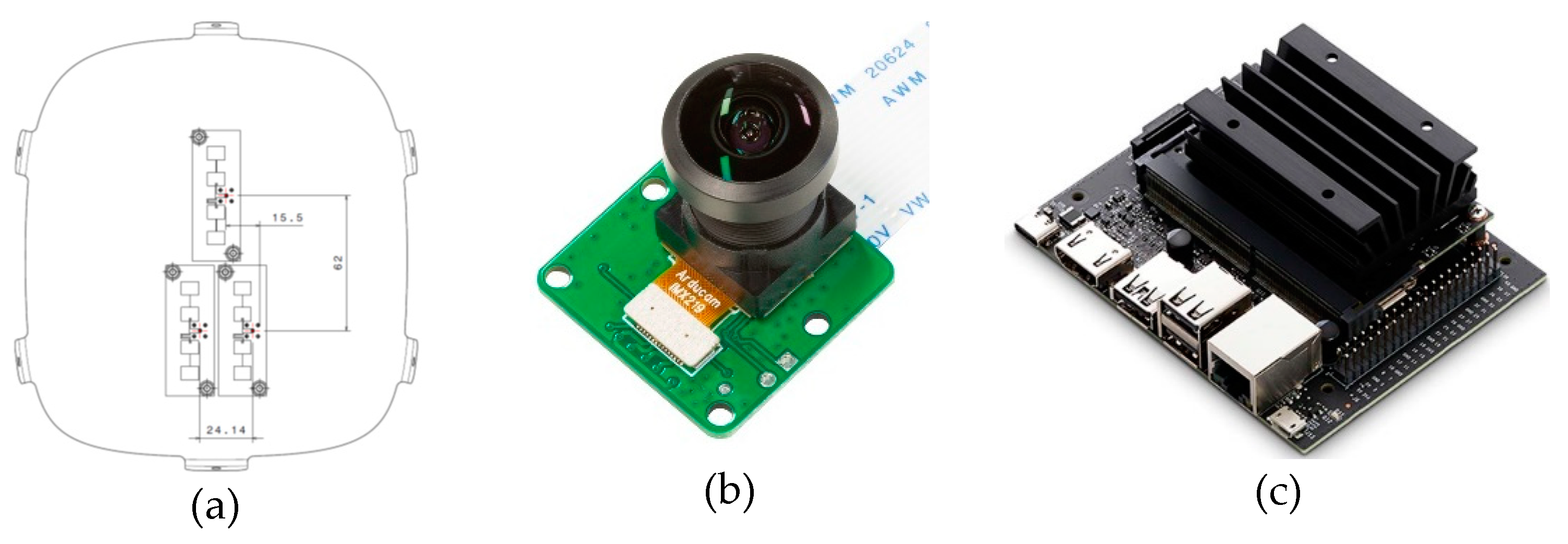
- Color camera Arducam 1/4” 8MP IMX219, 30 FPS. Recording resolution was set at 1280 x 720. Due to the small footprint size of the target in terms of pixels it was chosen a lens with a horizontal FOV of around .
- Sense and Avoid doppler radar, developed by Echoes.
- Vision Processing Unit. Nvidia Jetson Nano was chosen thanks to its small size and weight and low power absorption.
- Receiving and transmitting antennas are housed inside a fiberglass mockup of the nose of the aircraft to better simulate operating conditions of the system. Fig shows the position of the antennas within the nose. Camera sensor was mounted on the nose mockup in such a way to ensure the alignment of the camera Line of Sight with radar beam.
- Lipo batteries provide power to the radar at a tension of 22V, while a voltage regulator is employed to provide power to VPU and camera at a lower voltage.
- Two different workstations were used for real time monitoring of both radar and camera sensors.
Figure 27.
(a) Antennas placement within the nose mockup; (b) camera sensor chosen for the system implementation; (c) Jetson nano Vision Processing Unit.
Figure 27.
(a) Antennas placement within the nose mockup; (b) camera sensor chosen for the system implementation; (c) Jetson nano Vision Processing Unit.
During the flight test, each sensor was recording on a local storage the result of its own processing; moreover, a synchronization of radar processor and VPU with the system time of the telemetry onboard the aircraft was implemented to guarantee temporal alignment of data acquisition. Specifically, data acquired by each sensor during the test is summarized in Table 2.
Figure 28 shows the position of the Sense and Avoid system during the flight test with respect to the trajectory of the UAV. Tue blue line indicates the direction of the geographic north, the green line is parallel to the SAA LOS and the launch site of the drone is marked with a red rectangle. The drone was launched in the air leveraging its pneumatic catapult platform. It was decided to position the radar with the highway behind (visible in the lower right corner of the image) in order to reduce the ground clutter as much as possible. Radar sensor was designed for operation in the air where ground targets are not so close, thus during flight test some adjustments to the gains were made in order to compensate for the presence of cars and other highly reflective objects nearby. As noticeable in Figure 28, after take-off, the UAV entered an helicoidal climbing trajectory and then it remained in a Loiter circuit (approximately rectangular in shape) at a constant altitude of .
Telemetry data was post processed and transformed into a cartesian fixed Baseline Reference Frame (BRF), with its origin centred in the SAA system position and the x axis pointing north, axis towards right and chosen as to comply with the right-hand rule. The position of the UAV was reconstructed by the system in a cartesian Reference Frame fixed with the SAA system with axis oriented along the LOS. Attitude angles of the system as recorded by the IMU installed on the radar were used to transform position state recorded by the system in the BRF in order to compare them with telemetry. Figure 29 show one example of such reconstruction of the target position states, expressed in the BRF. Due to the presence of ground clutter, in certain section of the flights radar distance wasn’t available but optical algorithms still correctly performed detection and tracking. In absence of distance readings it was still possible to reconstruct heading and azimuth angles in camera reference frame. Figure 30 shows the comparison of said angles with ground truth (obtained by projecting the real UAV position logged by telemetry into the focus plane by means of camera intrinsic and extrinsic matrices) for two distinct segments of flight.
position state, (b) position state, (c) position state.
6. Conclusions
This paper has detailed the design and development of a sense and avoid system for a mini-UAV. The system was designed to comply with the strict SWaP constraints of the aircraft platform manufactured by SES. Particular focus was employed in the development of efficient processing algorithms with a sufficiently high refresh rate and ego motion compensation both for optical and radar sensor to ensure a robust detection and tracking capability. The developed, hardware in the loop, integrated simulation environment has allowed the validation of the sense and avoid algorithms for a multitude of different collision scenarios leveraging a realistic, real-time, dynamic representation of the scene. Finally, the preliminary flight test campaign has produced promising results for the reconstruction of the position states of a representative target aircraft despite its small size and ground clutter noise. Several aspects still need to be investigated and will constitute the core of an important future research effort. First of all, the interaction between the FCS and avoidance algorithms has not been tested because the system was static during flight tests and during simulations, attitude and position states of the UAV were considered known in advance. Attitude angles are essential for the correct reconstruction of target position in an inertial reference frame. Therefore, complete flight tests with two flying aircraft will be conducted in the future where the SAA system will be deployed onboard one of the UAVs. The interaction between FCS and SAA system will be validated during said flight campaign and the test will provide precious insights about the effectiveness of motion compensation capabilities in rejecting noise caused by the ego-motion of the platform and engine vibration. Future research will also investigate more advanced collision avoidance strategies, leveraging 3D manoeuvres with optimality constraints (fuel/time minimization). Another essential aspect to be investigated is the simultaneous presence of multiple intruder aircraft within the FOV, where possibly each of them pose a collision threat. Finally, the benefits of employing an array of camera sensors properly oriented to enlarge the overall available FOV will be investigated together with the utilisation of the coarse azimuth reading provided by the radar with the aim of increasing system capabilities and robustness w.r.t to noise.
Author Contributions
Conceptualization, R.G. and M.F.; methodology, R.G. and M.F.; software, M.F.; validation, R.G., G.D.R. and M.F.; formal analysis, R.G., G.D.R. and M.F.; investigation, M.F.; resources: R.G. and G.D.R.; data curation, M.F.; writing – original draft preparation, M.F.; writing - review and editing, R.G. and M.F; visualization, R.G., G.D.R. and M.F.; supervision, R.G. and M.F.; project administration, R.G.; funding acquisition, R.G. and G.D.R.. All authors have read and agreed to the published version of the manuscript.
Funding:This research was co-funded by the Italian Government (Ministero delle Imprese e del Made in Italy, MIMIT) and by the Tuscany Regional Government, in the context of the R&D project “Tecnologie Elettriche e Radar per SAPR Autonomi (TERSA)”, Grant number: F/130088/01- 05/X38. .
Data Availability Statement
Restriction apply to the availability of these data.
Acknowledgments
The authors wish to thank the project leader company Sky Eye Systems S.r.l. (Via Grecia 52, 56021 Cascina, Italy) for the support to the research activity and for providing the UAV aero-mechanical data and FCS laws that allowed the creation of an accurate dynamic simulation model. Special thanks to the partner company Echoes S.r.l. (Viale Giovanni Pisano 55, 56123 Pisa, Italy), responsible for the design and development of the SAA radar, and to the partner company Free Space S.r.l. (via Antonio Cocchi 7, 56121 Pisa, Italy) for the design and development of the radar antennas.
Conflicts of Interest
The authors declare no conflicts of interest. The funders had no role in the design of the study; in the collection, analyses, or interpretation of data; in the writing of the manuscript; or in the decision to publish the results.
References
- FAA “Integration of Civil Unmanned Aircraft Systems (UAS) in the National Airspace System (NAS) Roadmap - 2° Ed,” Federal Aviation Administration, 2018.
- R. Merkert and J. Bushell, “Managing the drone revolution: A Systematic literature review into the current use of airborne drones and future strategic directions for their effective control,” Journal of Air transport Management, 2020. [CrossRef]
- P. Angelov, Sense and Avoid in UAS (Research and Applications), John Wiley & Sons, Ltd ISBN: 978-0-470-97975-4, 2012.
- K. V. a. L. P. K. Dalamagkidis, “On unmanned aircraft systems issues, challeneges and operational restrictions preventing integration into the National Airspace System,” Progress in Aerospace Sciences, vol. 44, no. 7, pp. 503-519, 2008. [CrossRef]
- ENAC, “Regolamento mezzi aerei a pilotaggio remoto,” 2016.
- G. Recchia, G. Fasano, D. Accardo and A. Moccia, “An Optical Flow Based electro-Optical See-and-Avoid System for UAVs,” IEEE, 2007. [CrossRef]
- J. martin, J. Riseley and J. J. Ford, “A Dataset of Stationary, Fixed-wing Aircraft on a Collision Course for Vision-Based Sense and Avoid,” in International Conference on Unmanned Aircraft Systems (ICUAS), Dubrovnik, Croatia, 2022. [CrossRef]
- FAA, “Sense and Avoid (SAA) for unmanned aircraft systems (UAS). Prepared by FAA sponsored Sense and Avoid Workshop,” Oct. 9, 2009.
- Radio Technical Commision for Aeronautics, “RTCA-DO-185B, Minimum operational performance standards for traffic alert and collision avoidance system II (TCAS II),” July 2009.
- D. Klarer, A. Domann, M. Zekel, T. Schuster, H. Mayer and J. Henning, “Sense and Avoid Radar Flight Tests,” in International Radar Symposium, Warsaw, Poland, 2020. [CrossRef]
- M. Mohammadkarimi and R. T. Rajan, “Cooperative Sense and Avoid for UAVs using Secondary Radar,” IEEE transactions on aerospace and electronic systems, 2024. [CrossRef]
- A. Huizing, M. Heiligers, B. Dekker, J. d. Wit and L. Cifola, “Deep Learning for Classification of Mini-UAVs Using Micro-Doppler Spectrograms in Cognitive Radar,” IEEE Aerospace and Electronic Systems Magazine, vol. 34, no. 11, pp. 46-56, 2019. [CrossRef]
- Y. L. a. Y. S. “. a. t. o. a. U. v. C. Zhou, “Detection and tracking of a UAV via hough transform,” in CIE International Conference on Radar, 2016. [CrossRef]
- S. Ramasamy, R. Sabatini, A. Gardi and J. Liu, “LIDAR Obstacle Warning and Avoidance System for Unmanned Aerial Vehicle Sense-and-Avoid,” Aerospace Science and Technology, 2016. [CrossRef]
- v. Karampinis, A. Arsenos, O. Filippopoulos, E. Petrongonas, C. Skliros, D. Kollias, S. Kollias and A. Voulodimos, “Ensuring UAV Safety: A Vision-only and Real-time Framework for Collision Avoidance Through Detection, Tracking and Distance Estimation.,” in International Conference on Unmanned Aircraft Systems (ICUAS), Chania, Crete, Greece, 2024. [CrossRef]
- R. Opromolla, G. Inchingolo and G. Fasano, “Airborne Visual Detection and Tracking of Cooperative UAVs Exploiting Deep Learning,” MDPI Sensors, vol. 19, 2019. [CrossRef]
- J. Zhao, J. Zhang, D. Li and D. Wang, “Vision-based Anti-UAV Detection and Tracking,” IEEE Transactions on Intelligent Transportation Systems, 2022. [CrossRef]
- P. Bauer, A. HIba and J. Bokor, “Monocular Image-based Intruder Direction Estimation at Closest Point of Approach,” in International COnference on Unmanned Aircraft Systems (ICUAS), Miami, FL, USA, 2017. [CrossRef]
- F. Vitiello, F. Causa, R. Opromolla and G. Fasano, “Experimental Analysis of Radar/Optical Track-to-track Fusion for Non-Cooperative Sense and Avoid,” in International COnference on Unmanned Aircraft Systems (ICUAS), Warsaw, Poland, 2023. [CrossRef]
- G. Fasano, D. Accardo, A. E. Tirri and A. Moccia, “Radar/electro-optical data fusion for non-cooperative UAS sense and avoid,” Aerospace Science and Technology, vol. 46, pp. 436-450, 2015. [CrossRef]
- ICAO, “Doc 10019 - Manual on Remotely Piloted Aircraft Systems,” International Civil Aviation Organization, 2015.
- ICAO, “Cir. 328 - Unmanned Aircraft Systems (UAS),” International Civil Aviation Organization, 2011, 2011.
- ASTM Designation: F 2411-04, “Standard Specification for Design and Performance of an Airborne Sense-and-Avoid system,” ASTM International, West Conshohocken, PA, 2004.
- EUROCONTROL, “Specification for the use of Military Unmanned Aerial Vehicle as Operational Traffic Outside Segregated Airspaces, SPEC-0102,” July 2007.
- A. D. Zeitlin, “Progress on Requirements and Standards for Sense & Avoid,” The MITRE Corporation, 2010.
- C. Geyer, S. Singh and L. Chamberlain, “Avoiding Collisions Between Aircraft: State of the Art and Requirements for UAVs operating in Civilian Airspace.,” 2008.
- G. Fasano, D. Accado, A. Moccia and D. Moroney, “Sense and Avoid for Unmanned Aircraft Systems,” IEEE A&E SYSTEMS MAGAZINE, pp. 82-110, November 2016. [CrossRef]
- S. Ramasmy and R. Sabatini, “A Unified Approach to Cooperative and Non-Cooperative Sense-and-Avoid,” in International Conference on Intelligent robots and Systems (IROS), Vancouver, BC, Canada, 2017. [CrossRef]
- B. D. Lucas and T. Kanade, “An Iterative Image Registration Technique with an Application to Stereo Vision,” in Proceedings of the 7th International Joint Conference on Artificial Intelligence, Vancouver, Canada, 1981.
- C. Harris and M. Stephens, “A Combined Corner And Edge Detection,” in Proceedings of the 4th Alvey Vision Conference, 1988. [CrossRef]
- J. Y. Bouguet, “Pyramidal Implementation of the Lucas Kanade Feature tracker Description of the algorithm,” Intel Corporation, Microprocessor Research Labs, 2000.
- L. Forlenza, G. Fasano and A. M. D. Accardo, “Flight Performance Analysis of an Image Processing Algorithm for Integrated Sense-and-Avoid Systems,” International Journal of Aerospace Engineering, p. 8, 2012. [CrossRef]
- Y. Benezeth, P. M. Jodoin, B. Emile, H. Laurent and C. Rosenberger, “Comparative Study of Background Subtraction Algorithm,” Journal of Electronic Imaging, July 2010. [CrossRef]
- J. Redmon, S. Divvala, R. Girshick and A. Farhadi, “You Only Look Once: Unified Real-Time Object Detection,” 9 May 2016. [Online]. Available: https://arxiv.org/abs/1506.02640v5.
- S. W. Kim, K. Yun, K. M. Yi, S. J. Kim and J. Y. Choi, “Detection of moving objects with moving camera using non-panoramic background model,” machine Vision and Applications, pp. 1016-1028, 2013. [CrossRef]
- W. Y. D. H.,. J. K. L. Kurnianggoro, “Online Backgorund-Subtraction with Motion Compensation for Freely Moving Camera.,” in Intelligent Computing Theories and Application, 2016. [CrossRef]
- K. M. Yi, K. Yun, S. W. Kim, H. J. Chang, H. Jeong and J. Y. Choi, “Detection of Moving Objects with Non-stationary Cameras in 5.8ms: Bringing Motion Detection to Your Mobile Device,” in IEEE Conference on Computer Vision and Pattern Recognition Workshops, 2013. [CrossRef]
- C. Carbone, U. Ciniglio, F. Corraro and S. Luongo, “A Novel 3D Geometric Algorithm for Aircraft Autonomous Collision Avoidance,” in Proceedings of the 45th IEEE Conference on Decision and Control, San Diego, CA, USA, 2006. [CrossRef]
- A. Chakravarthy and D. Ghose, “Obstacle avoidance in a Dynamic Environment: A Collision Cone Approach,” IEEE Transactions on Systems, Man and Cybernetics - Part A: Systems and Humans, vol. 28, no. 5, 1998. [CrossRef]
- S. Wang, A. Then and R. Herschel, “UAV Tracking based on Unscented Kalman FIlter for Sense and Avoid Applications,” in International Radar Symposium, Warsaw, Polan, 2020. [CrossRef]
- H. Huang, H. Zhou, M. Zheng, C. Xu, X. Zhang and W. Xiong, “Cooperative Collision Avoidance Method for Multi-UAV Based on Kalman Filter and Model Predictive Control,” in International Conference on Unmanned Systems and Artificial Intelligence (ICUSAI), Xi'an, China, 2019. [CrossRef]
- M. Fiorio, R. Galatolo and G. D. Rito, “Extended Kalman Filter Based Data Fusion Algorithm Implemented in a Sense and Avoid System for a Mini-UAV application,” in IEEE Metrology for Aerospace, Lublin, Poland, 2024. [CrossRef]
Figure 1.
Reference TERSA aircraft.
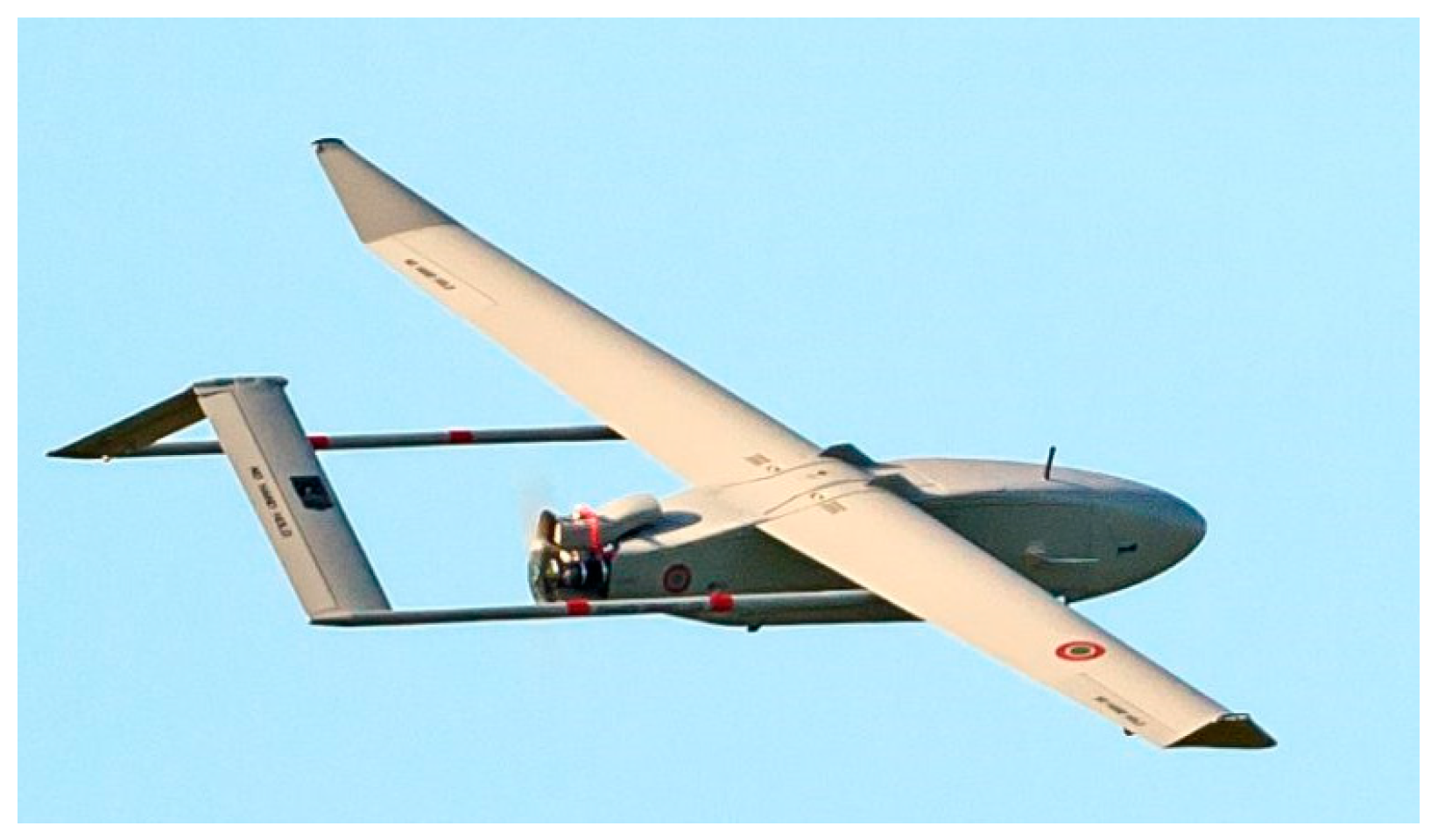
Figure 2.
a) minimum turn radius as a function of aerodynamic, structural and propulsive constraint for TERSA aircraft; (b) minimum detection required range as a function of intruder aircraft airspeed.
Figure 2.
a) minimum turn radius as a function of aerodynamic, structural and propulsive constraint for TERSA aircraft; (b) minimum detection required range as a function of intruder aircraft airspeed.
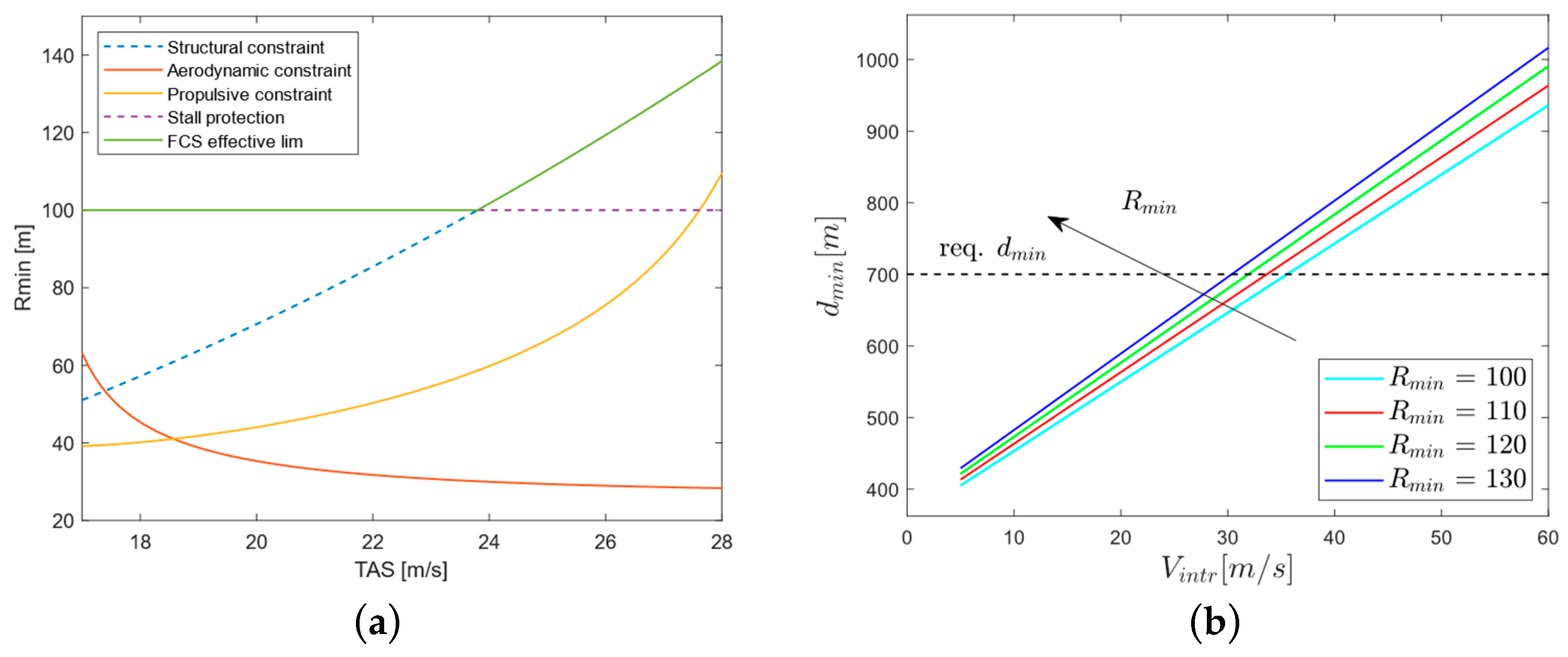
Figure 3.
Maximum attainable flight path angle @
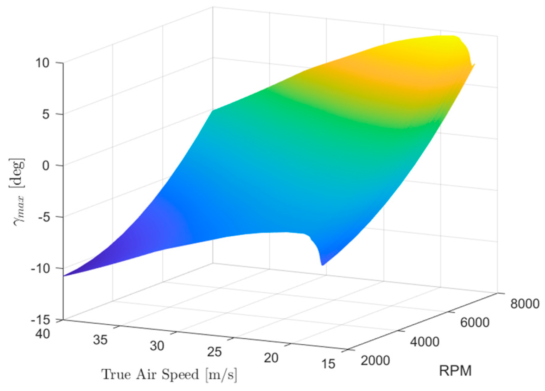
Figure 4.
SAA typical system integration high-level scheme.
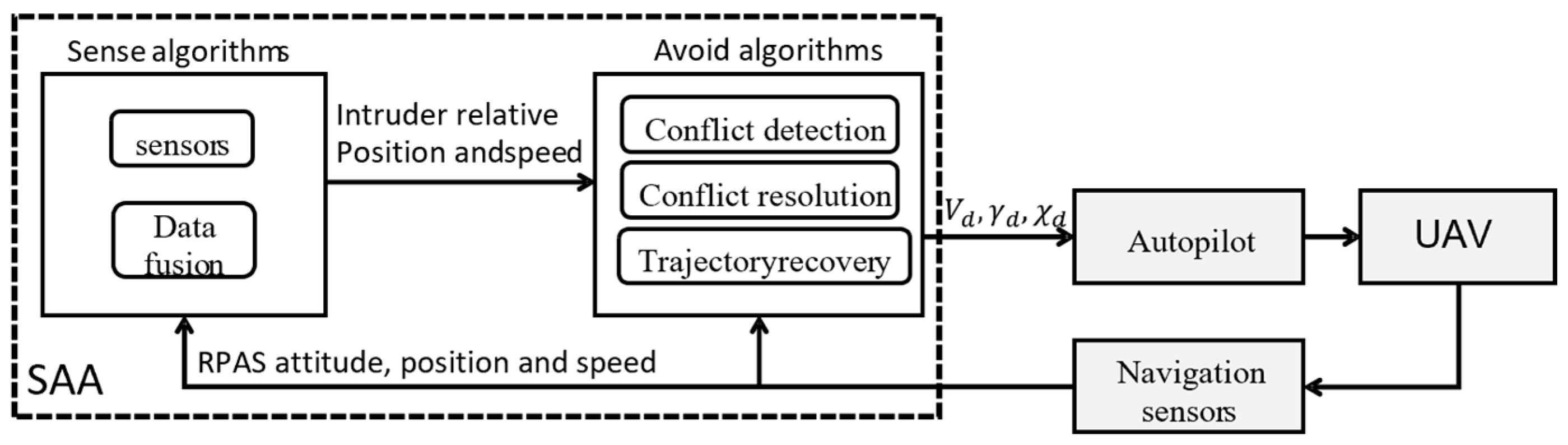
Figure 5.
High-level schematics of the proposed SAA system.
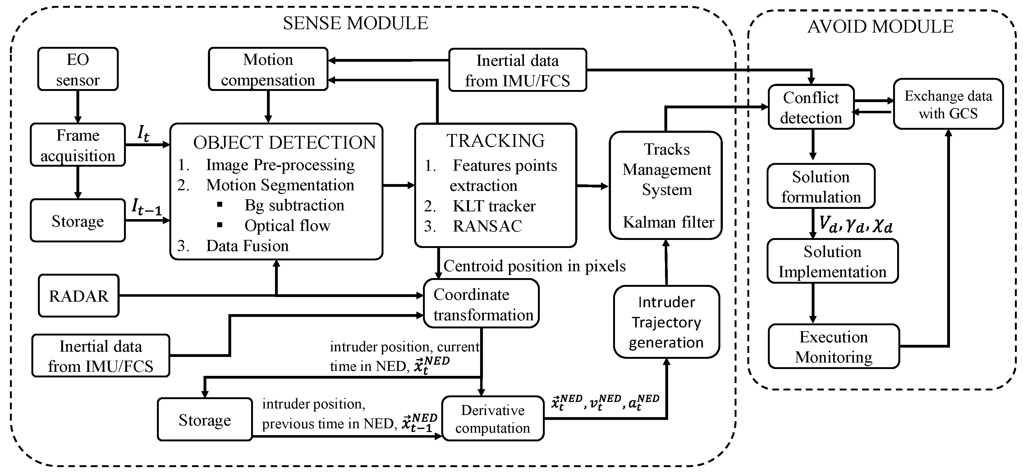
Figure 6.
Intruder aircraft azimuth and elevation angles reconstruction.
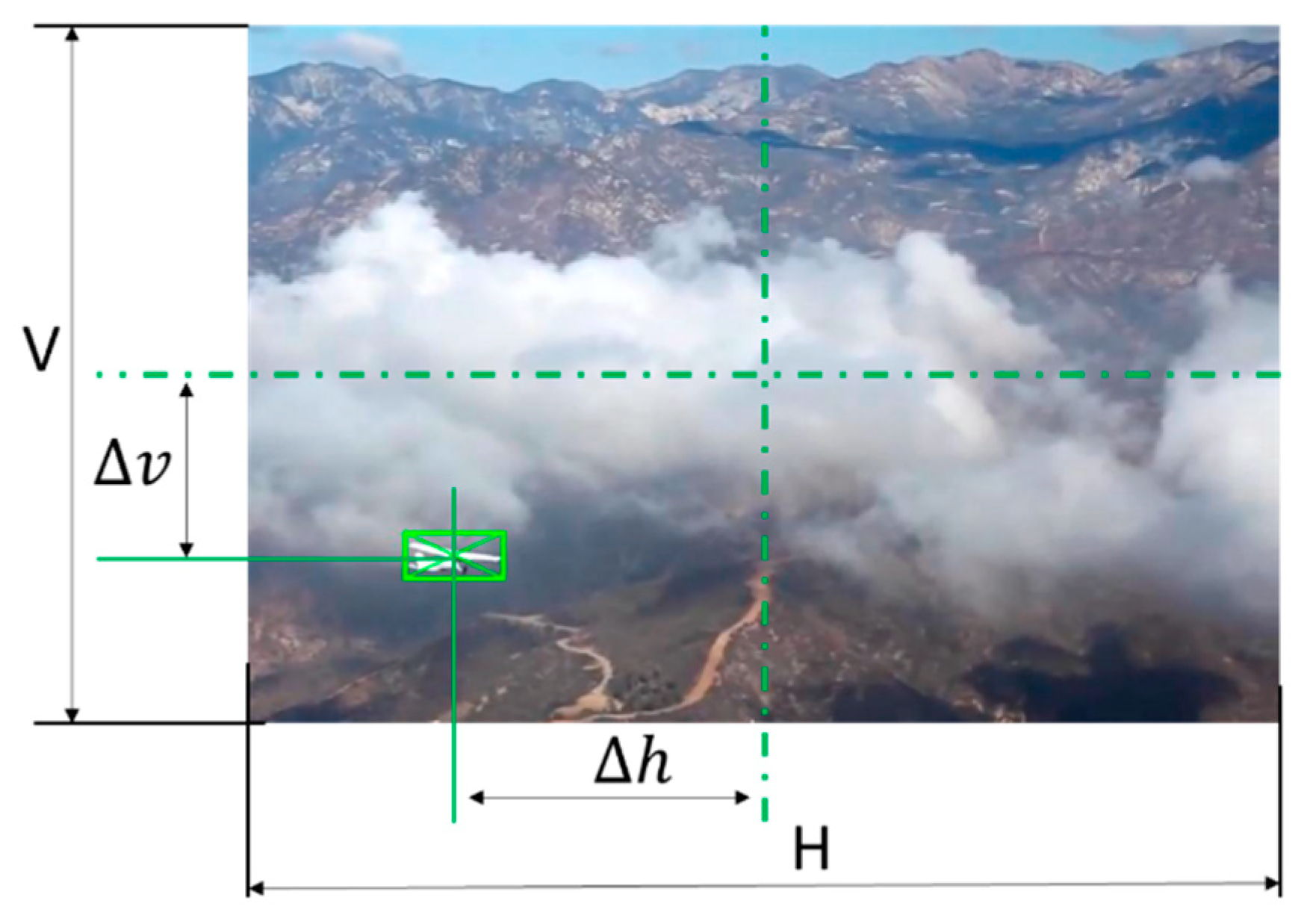
Figure 7.
Sense module computer vision pipeline.
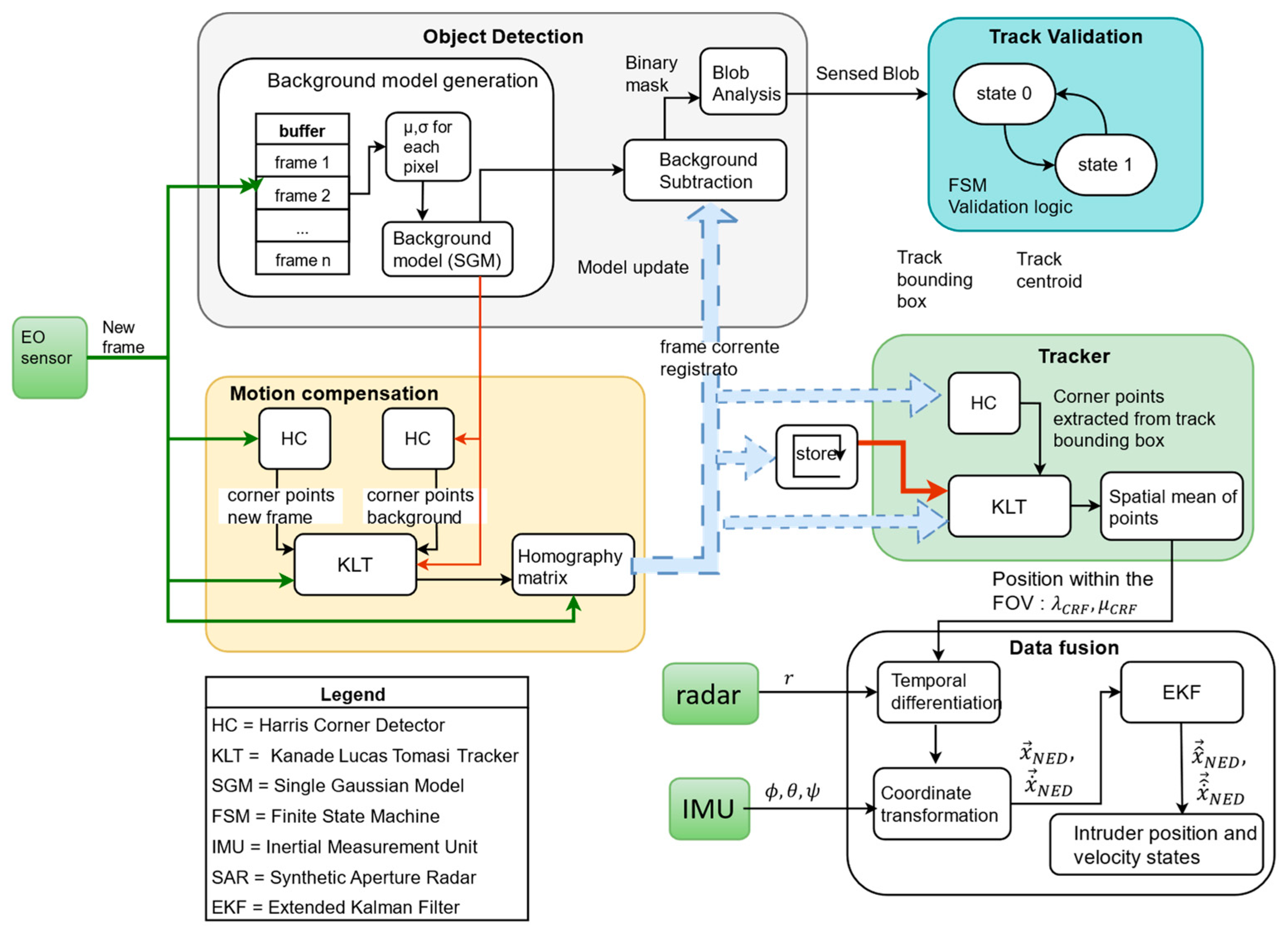
Figure 8.
Visual representation of the pyramidal expansion of the algorithm.
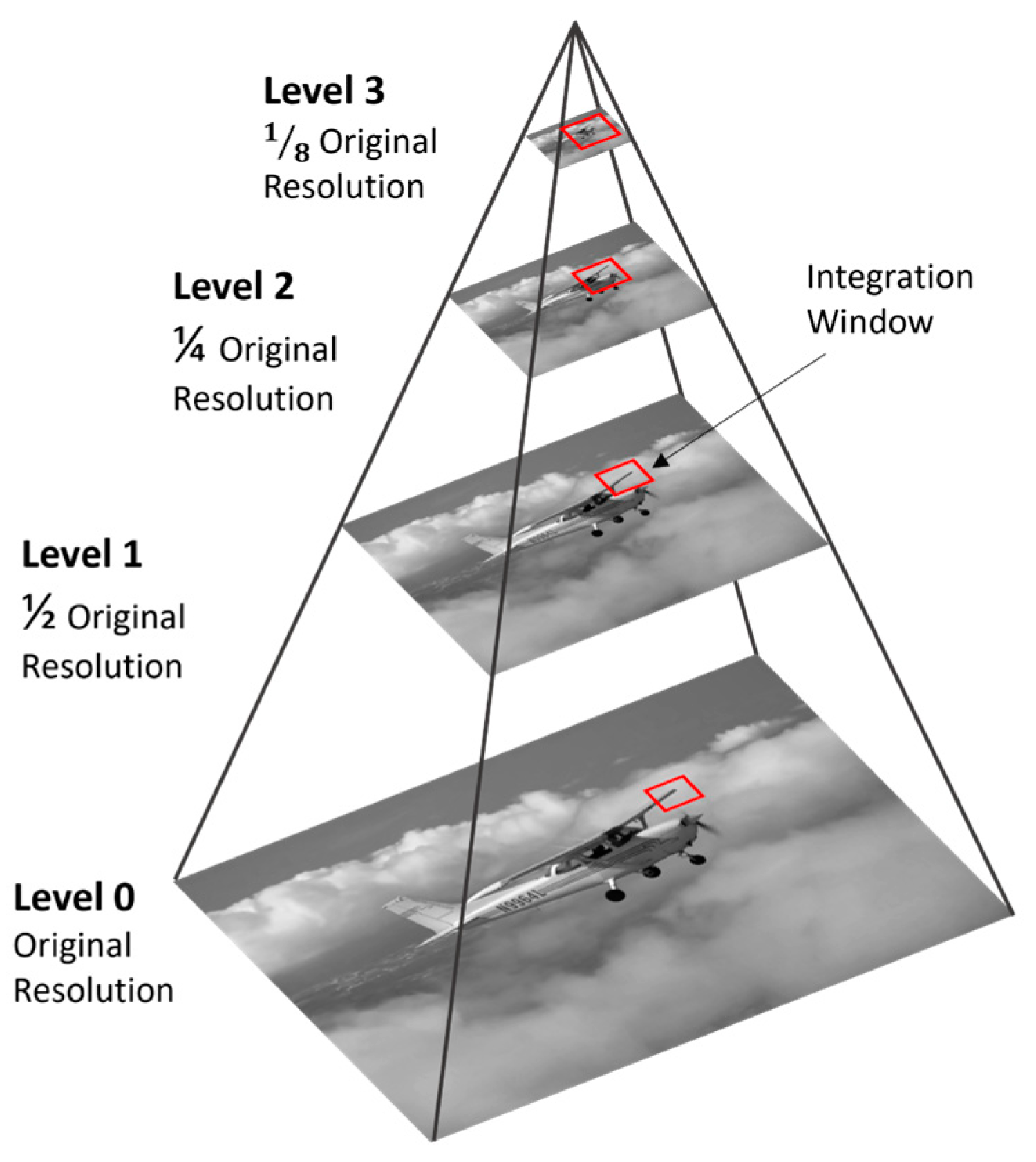
Figure 9.
Example of KLT feature matcher output.
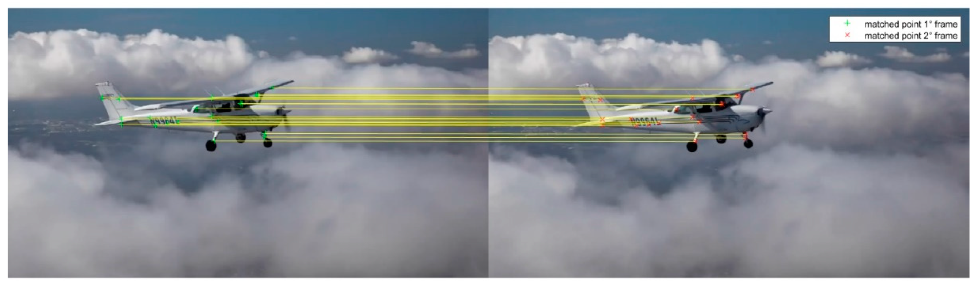
Figure 10.
Flow chart of KLT algorithm.
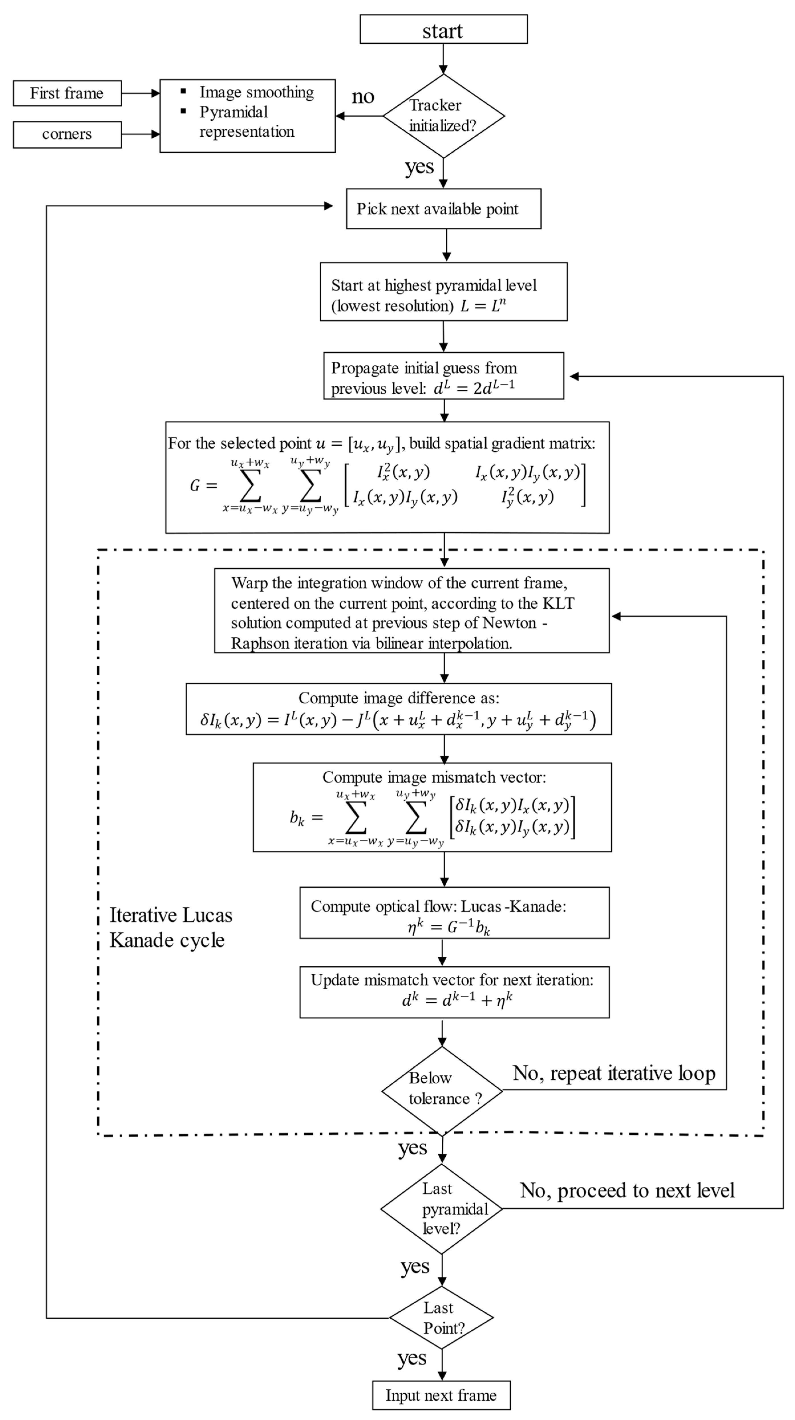
Figure 11.
High level scheme of the Finite State Machine handling the conflict detection and resolution problem.
Figure 11.
High level scheme of the Finite State Machine handling the conflict detection and resolution problem.
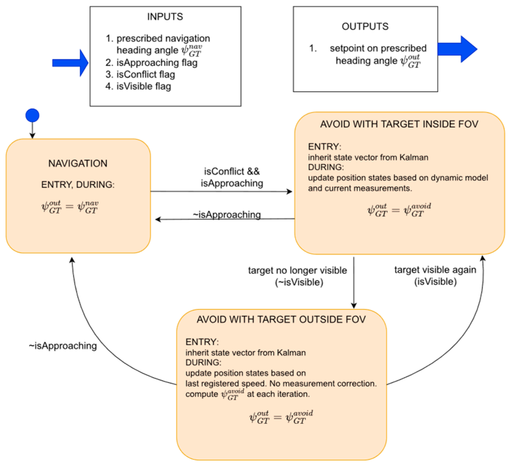
Figure 12.
Radar signal processing architecture.
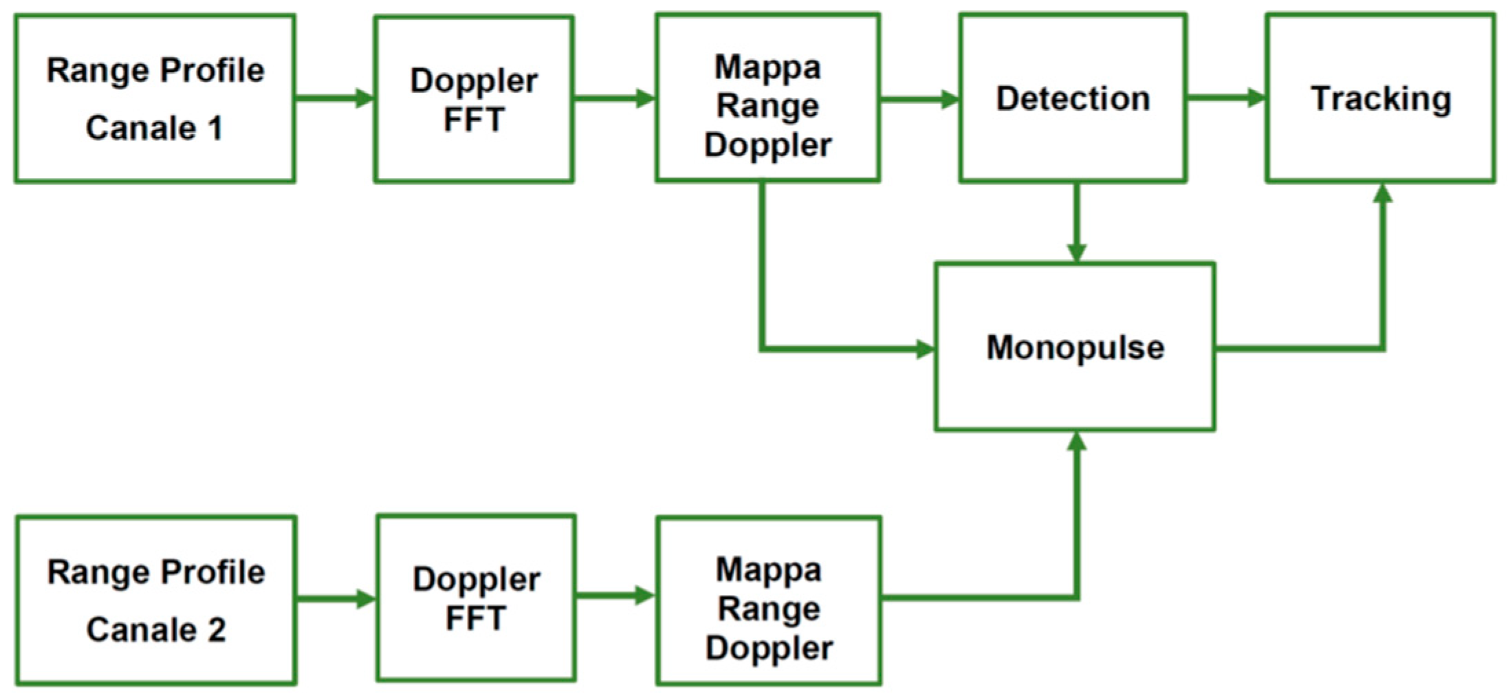
Figure 13.
(a) example of a range doppler map, (b) CFAR technique, (c) CA-CFAR technique.
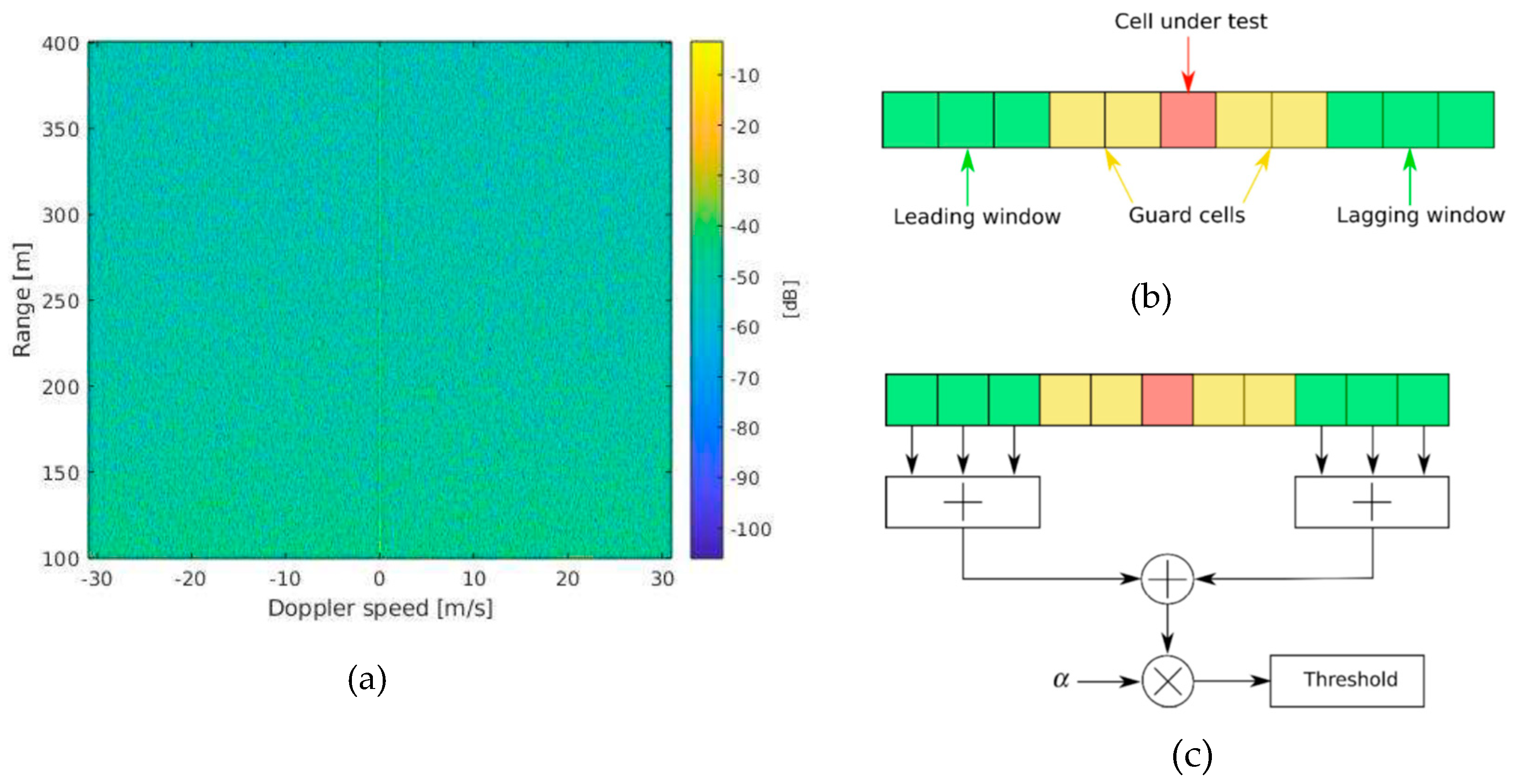
Figure 14.
(a) bi-dimensional CFAR; (b) binary mask showing detected tracks.
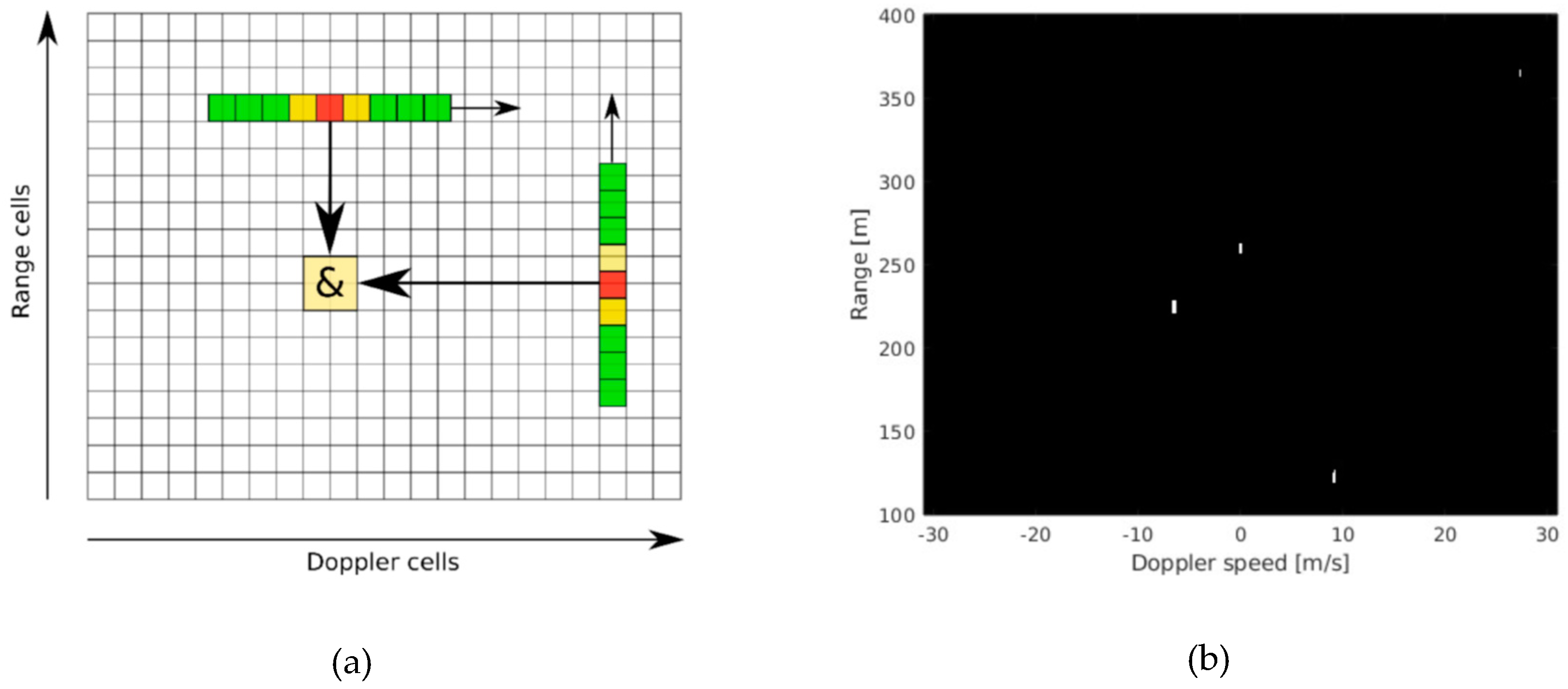
Figure 15.
Phase monopulse configuration.
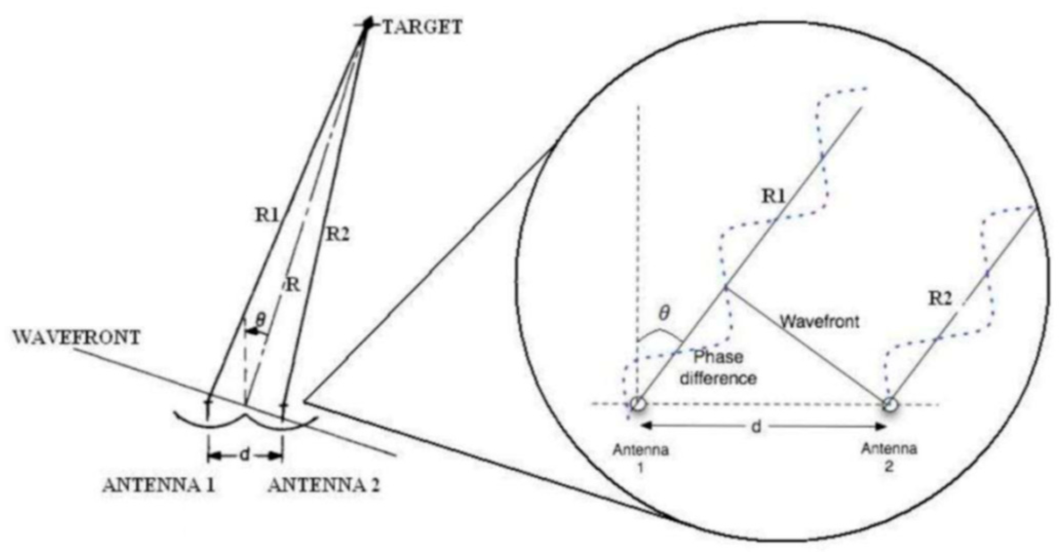
Figure 16.
Metrics used for the evaluation of avoidance manoeuvre (a); initial position of the intruder aircraft (b).
Figure 16.
Metrics used for the evaluation of avoidance manoeuvre (a); initial position of the intruder aircraft (b).
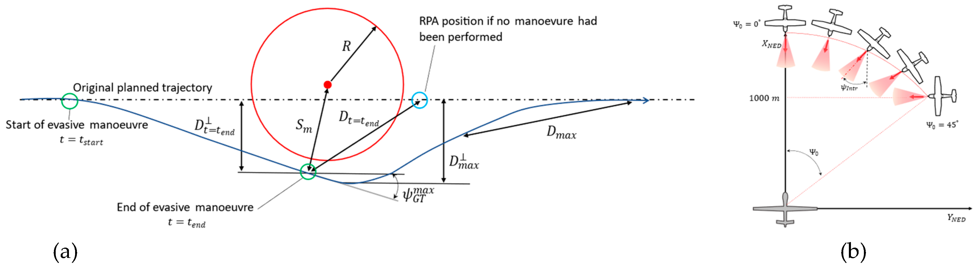
Figure 17.
Results of evasive maneuver for different initial positions and velocity states of the intruder aircraft; (a) 2D trajectory, (b) aileron deflection.
Figure 17.
Results of evasive maneuver for different initial positions and velocity states of the intruder aircraft; (a) 2D trajectory, (b) aileron deflection.
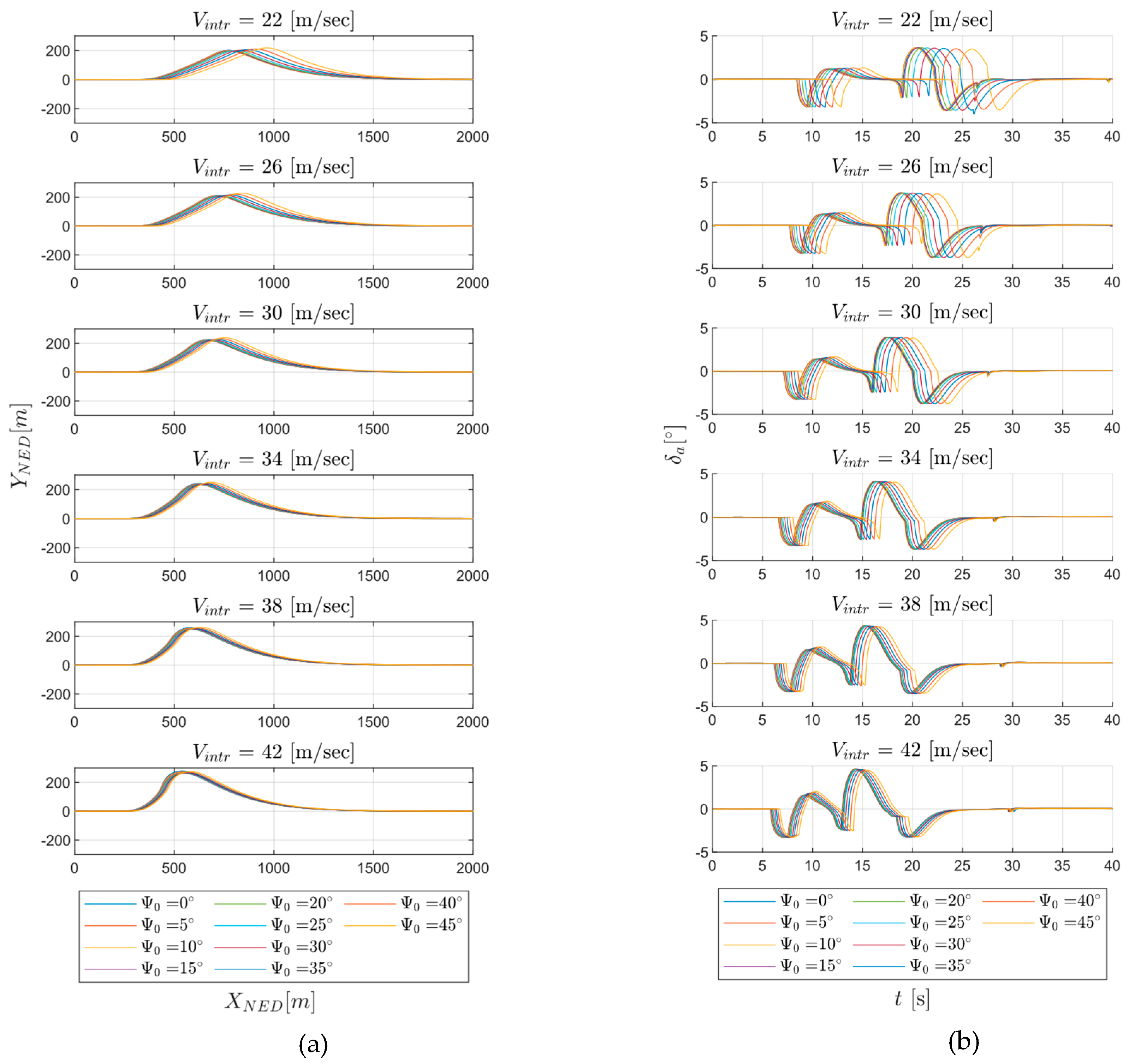
Figure 18.
Simulations Results; (a) minimum distance; (b) maximum normal deviation.
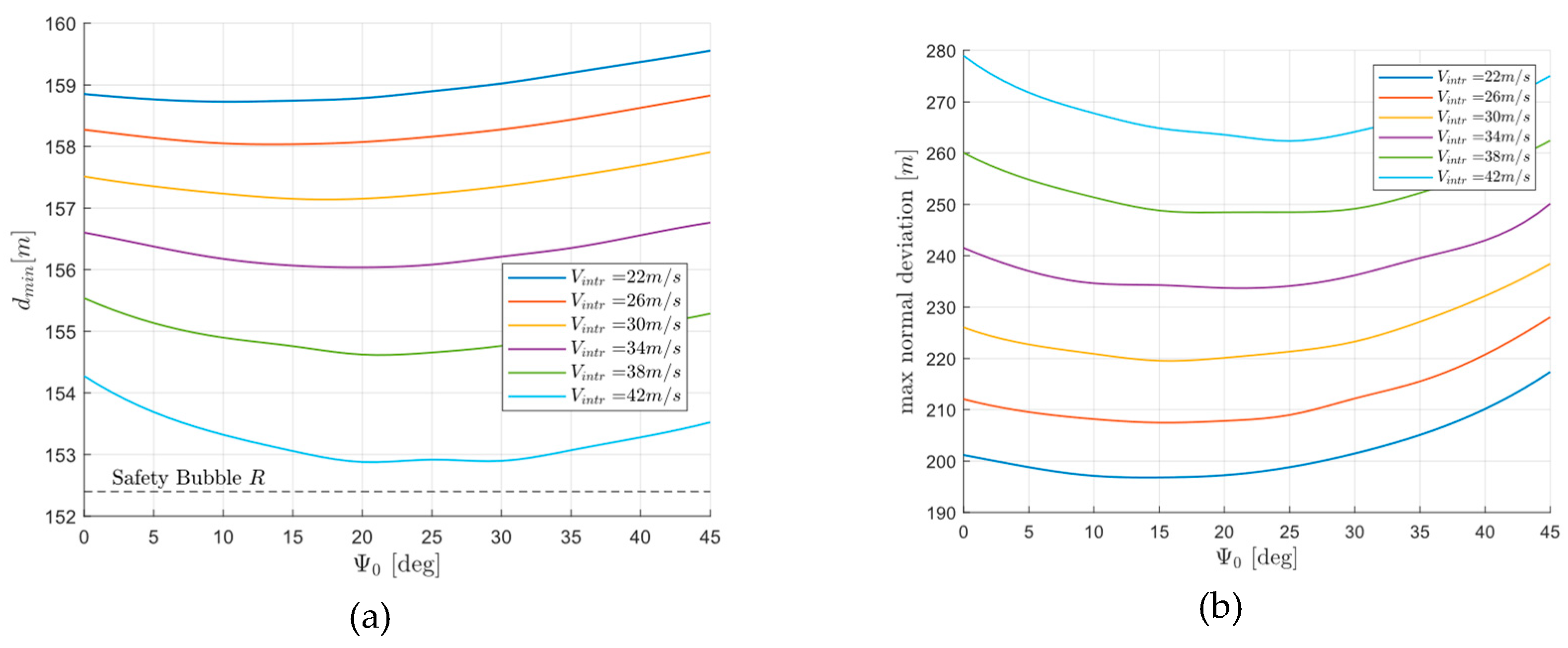
Figure 19.
Intruder position states (a,b,c) and velocity states (d,e,f) reconstruction by the EKF for a starboard encounter;
Figure 19.
Intruder position states (a,b,c) and velocity states (d,e,f) reconstruction by the EKF for a starboard encounter;
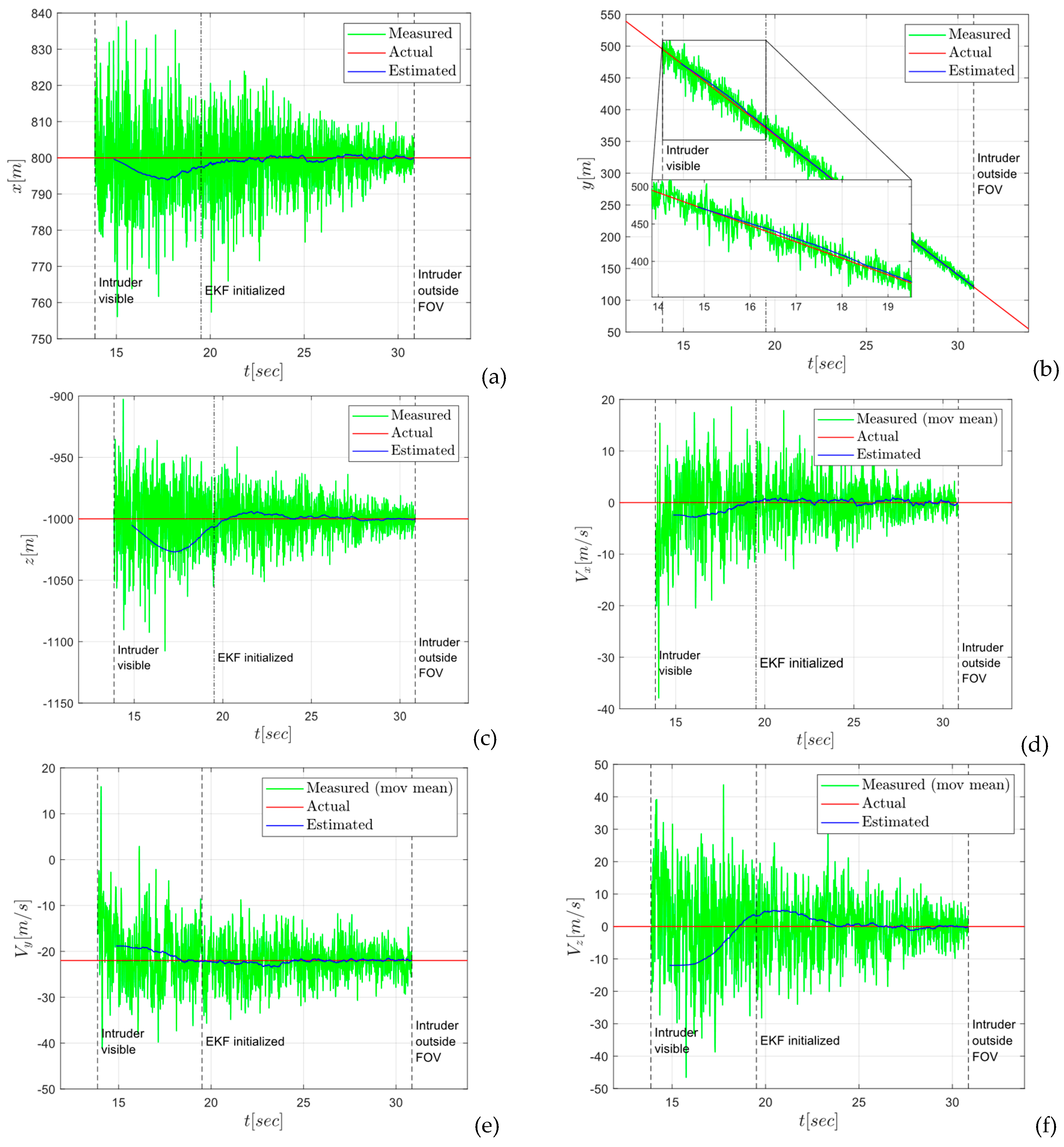
Figure 20.
High level scheme of the complete simulation framework.
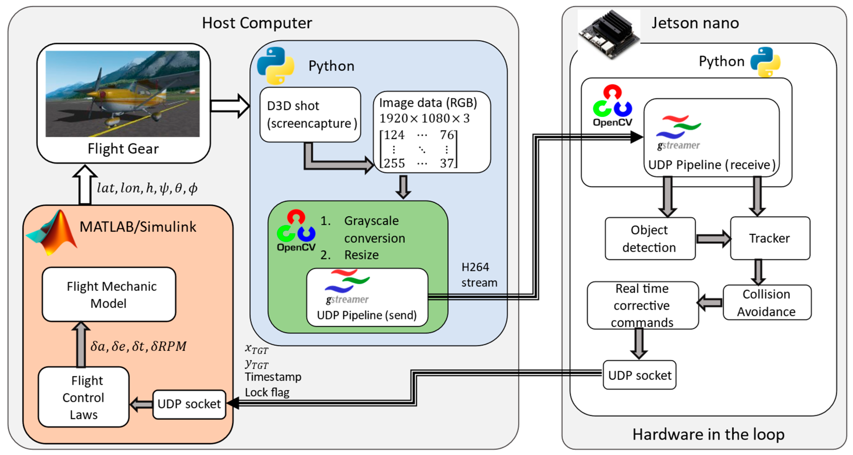
Figure 21.
Video stream send (a) and receive (b) pipeline schematics.
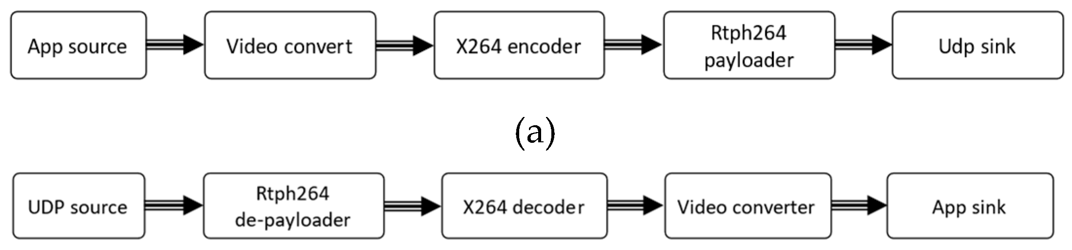
Figure 22.
SAA camera viewpoint as rendered in Flight Gear, (flying over the city of Pisa).
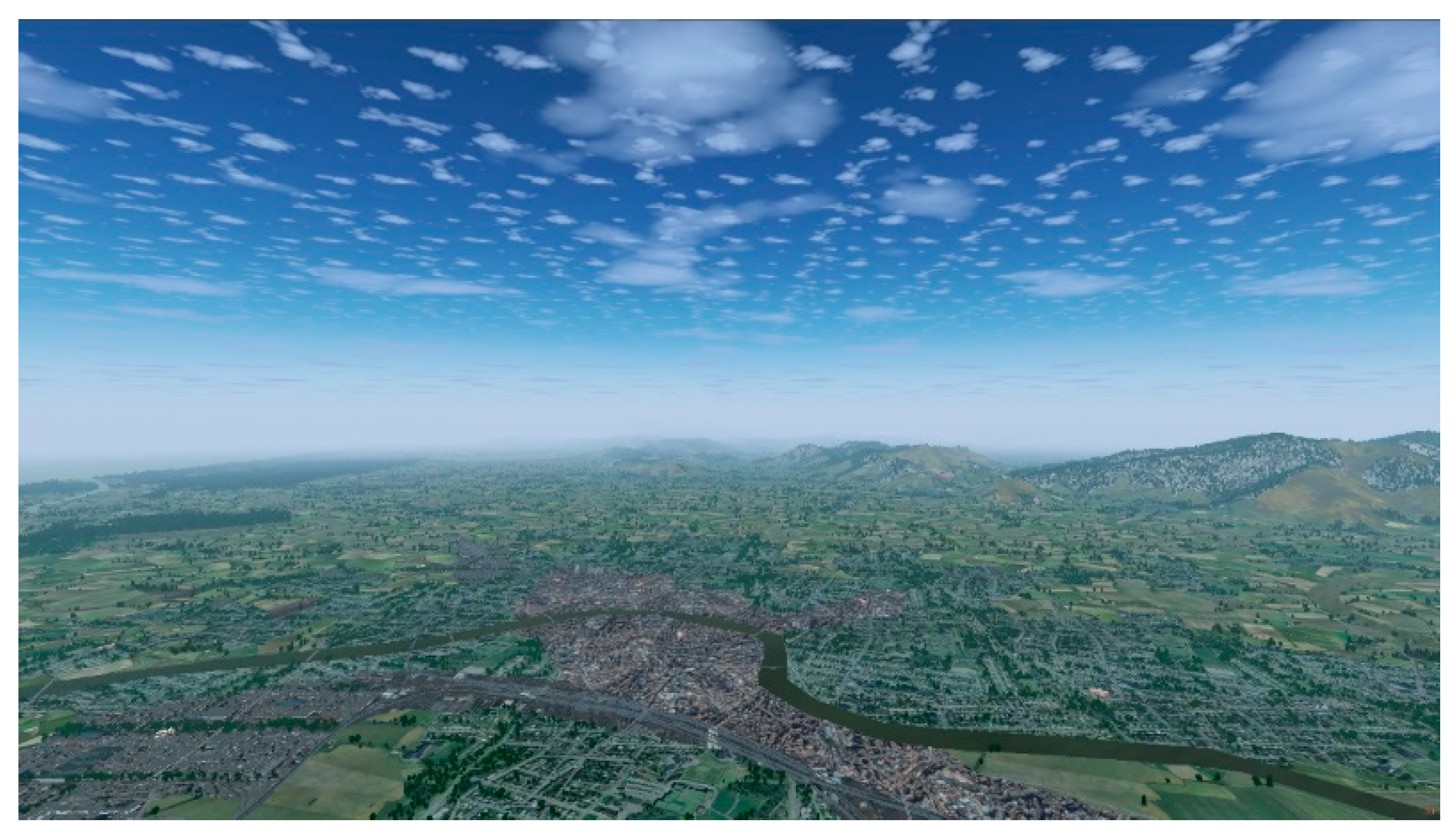
Figure 23.
Results of a HIL collision scenario in the complete simulation environment. Intruder approaching from starboard side.
Figure 23.
Results of a HIL collision scenario in the complete simulation environment. Intruder approaching from starboard side.
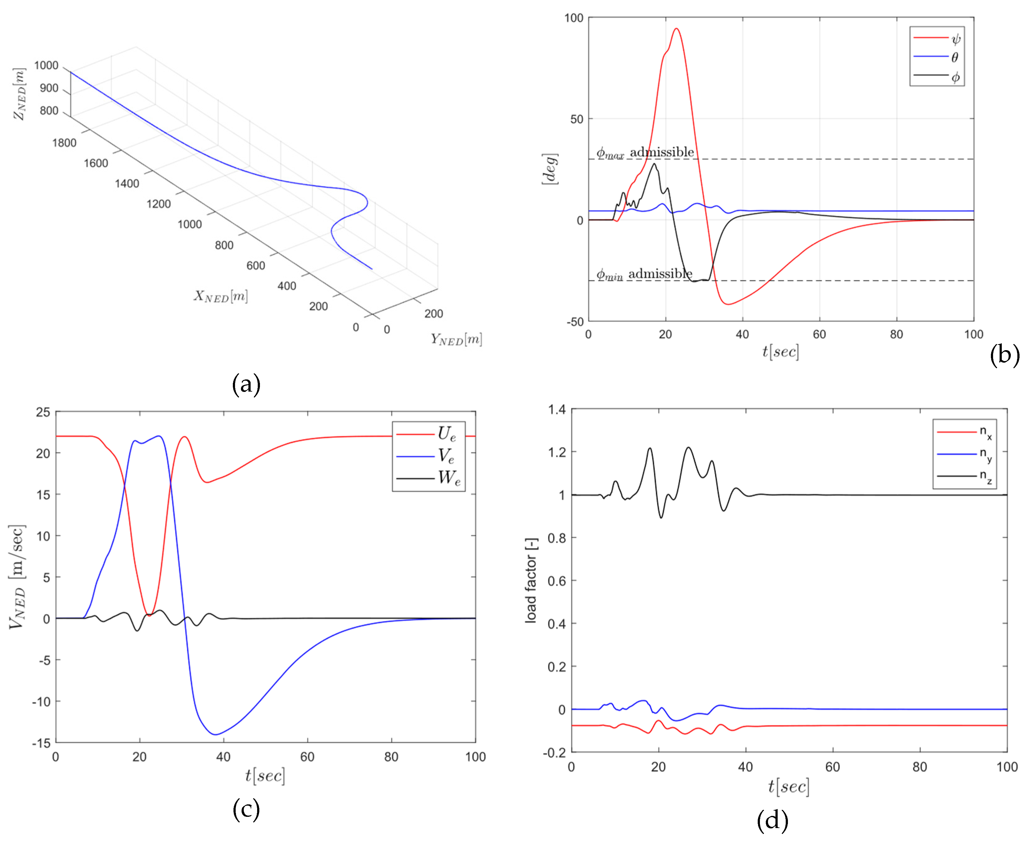
Figure 24.
Comparison between elevation (a) and azimuth (b) measurements with ground truth for the complete simulation framework.
Figure 24.
Comparison between elevation (a) and azimuth (b) measurements with ground truth for the complete simulation framework.
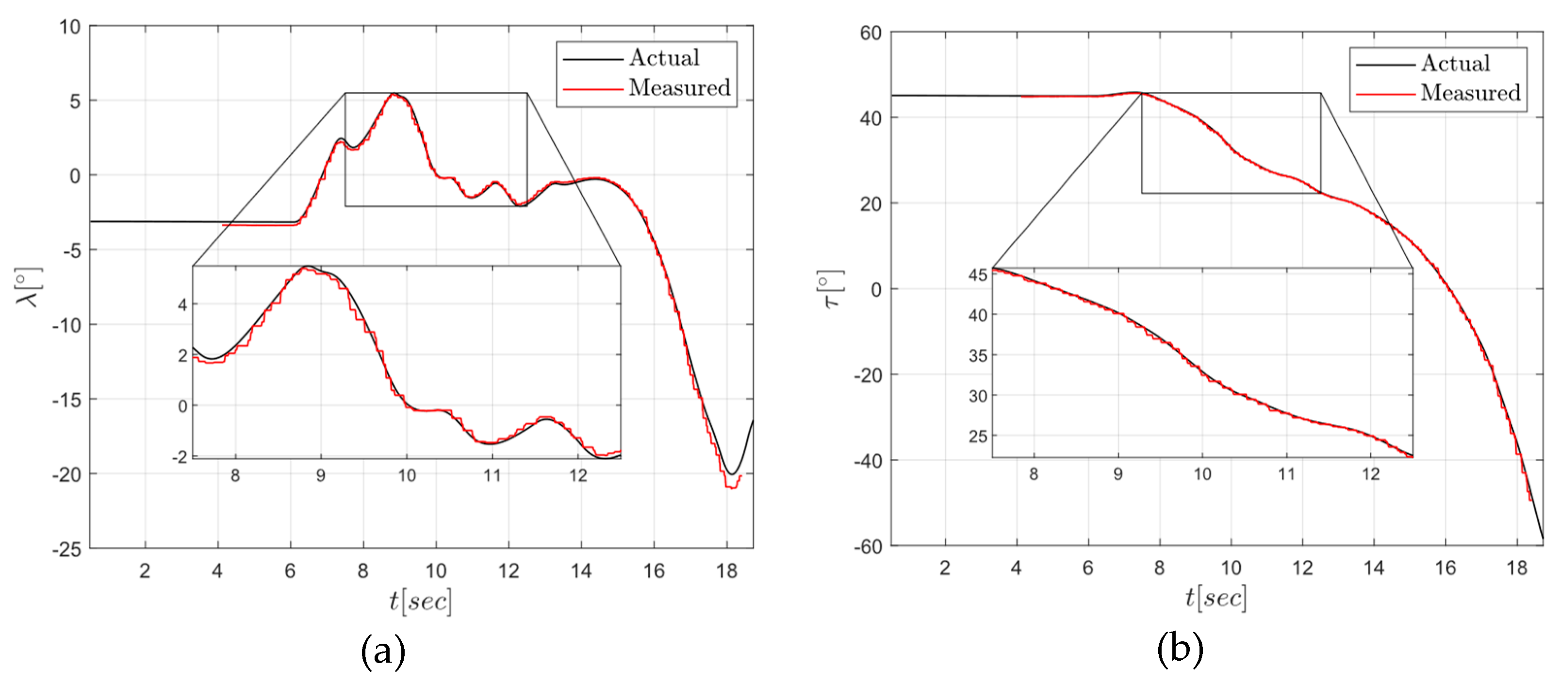
Figure 25.
Flight Gear Rendering of a starboard collision scenario on a coastal landscape with intruder position highlighted as detected by Sense algorithms within the complete simulation framework.
Figure 25.
Flight Gear Rendering of a starboard collision scenario on a coastal landscape with intruder position highlighted as detected by Sense algorithms within the complete simulation framework.
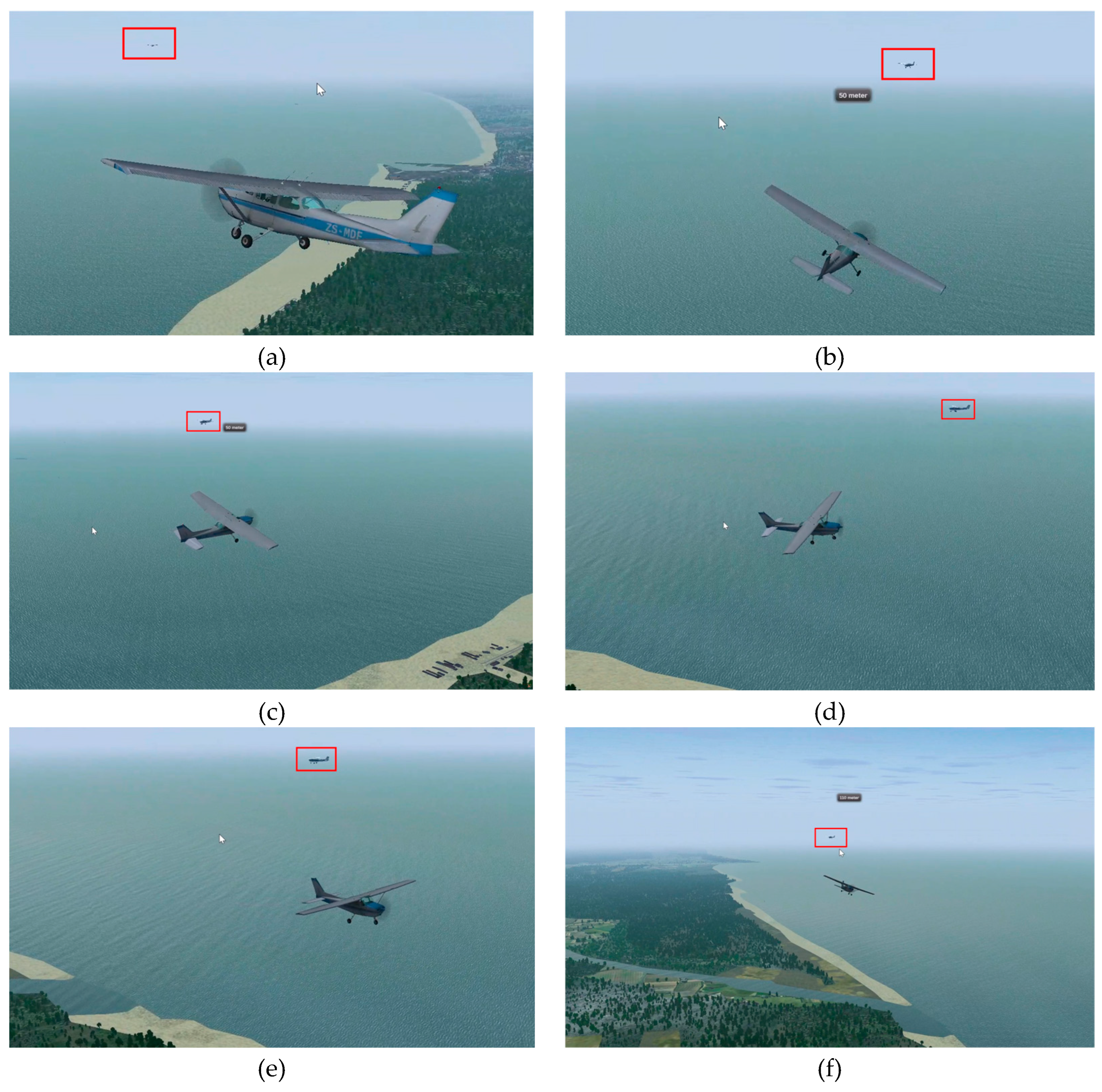
Figure 26.
SAA system prototype.
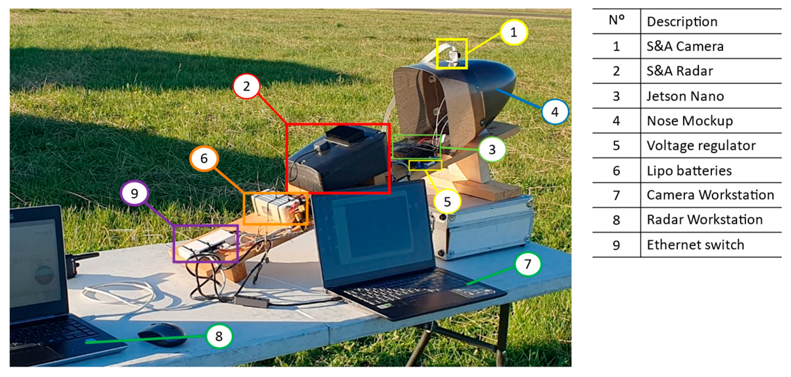
Figure 28.
SAA system position and UAV trajectory during flight test at Lucca-Tassignano airport.
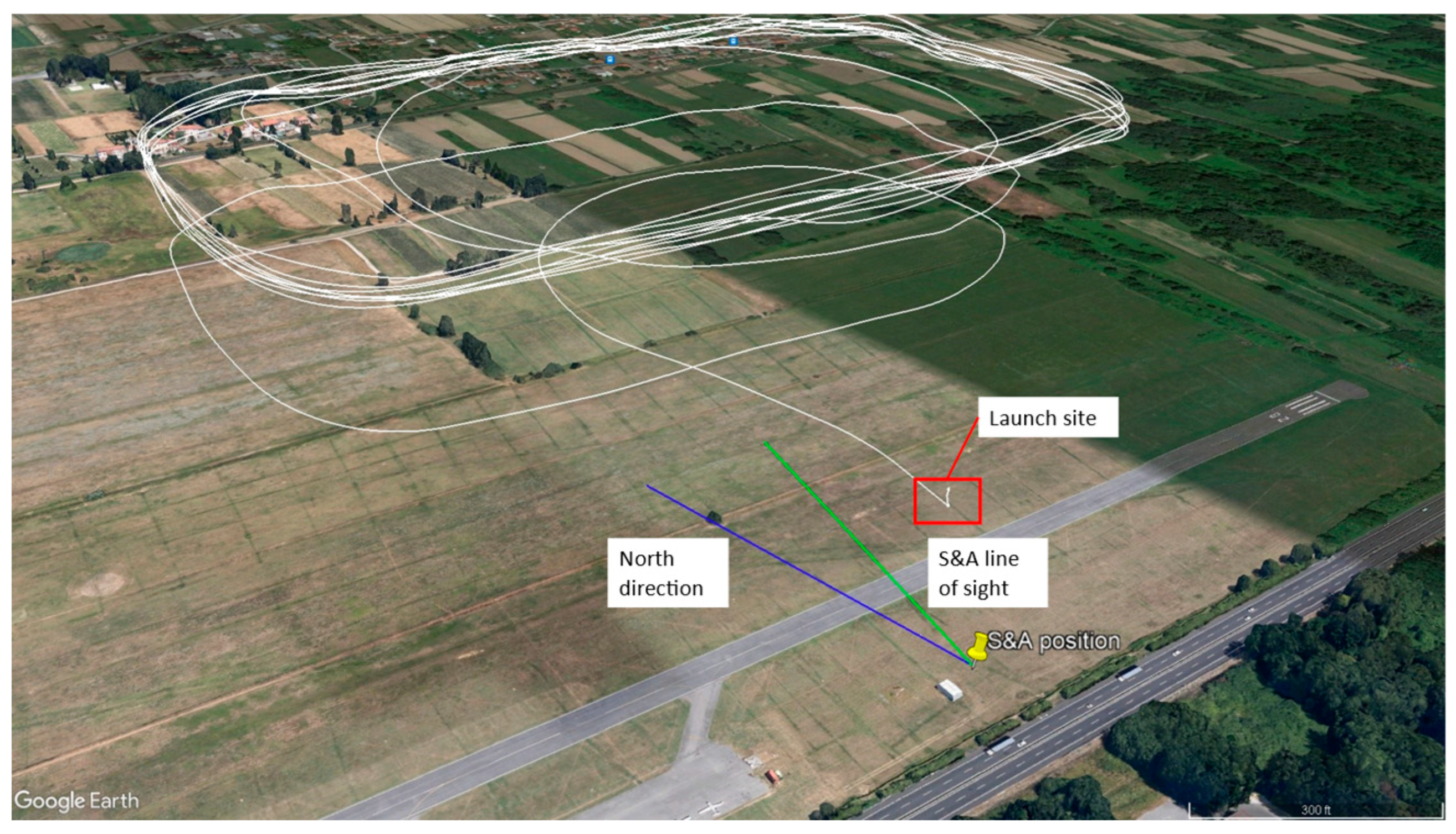
Figure 29.
reconstructed UAV position states vs telemetry in Base Reference Frame: (a)
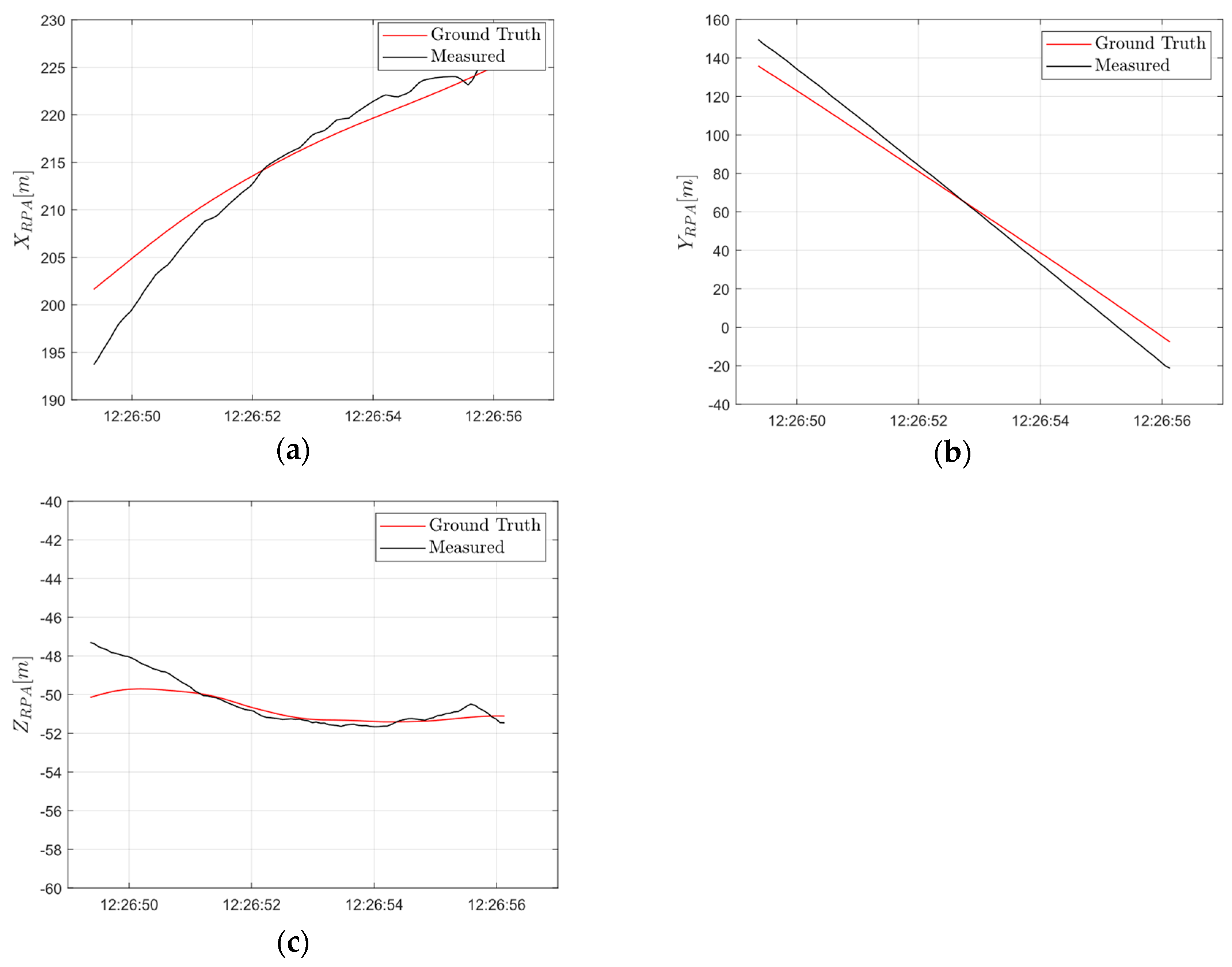
Figure 30.
relative azimuth (a) (c) and elevation (b) (d) angles between target UAV and SAA reference frame for two different flight phases.
Figure 30.
relative azimuth (a) (c) and elevation (b) (d) angles between target UAV and SAA reference frame for two different flight phases.
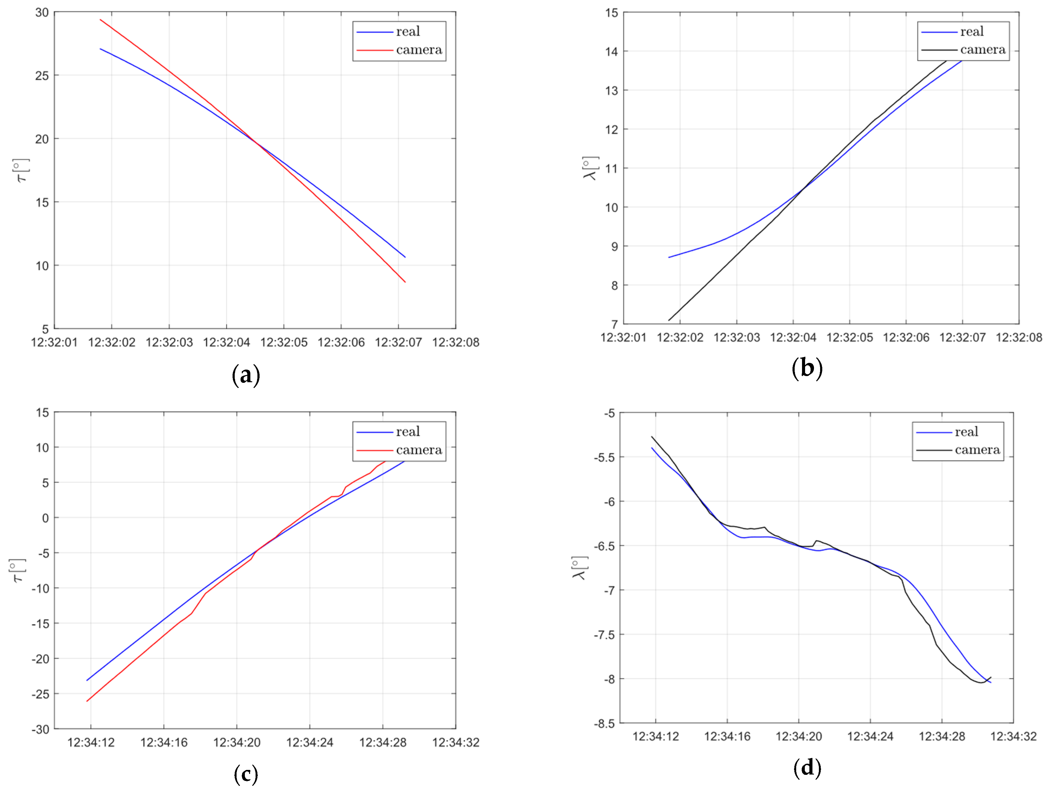

Table 1.
Reference aircraft characteristics.
| MTOW | |
| Reference surface S | |
| Mean aerodynamic chord | |
| Wingspan | |
| Stability margin |
Table 2.
Sensors data acquired during the flight test.
| UAV Telemetry | Radar | Camera |
|---|---|---|
| Altitude | Target radial distance | Target position within FOV |
| Latitude | Target radial velocity | Timestamp of readings |
| Longitude | System attitude (roll, pitch, heading) | |
| Timestamp of readings | System position (altitude, latitude, longitude) | |
| Timestamp of readings |
Disclaimer/Publisher’s Note: The statements, opinions and data contained in all publications are solely those of the individual author(s) and contributor(s) and not of MDPI and/or the editor(s). MDPI and/or the editor(s) disclaim responsibility for any injury to people or property resulting from any ideas, methods, instructions or products referred to in the content. |
© 2024 by the authors. Licensee MDPI, Basel, Switzerland. This article is an open access article distributed under the terms and conditions of the Creative Commons Attribution (CC BY) license (https://creativecommons.org/licenses/by/4.0/).
Copyright: This open access article is published under a Creative Commons CC BY 4.0 license, which permit the free download, distribution, and reuse, provided that the author and preprint are cited in any reuse.


