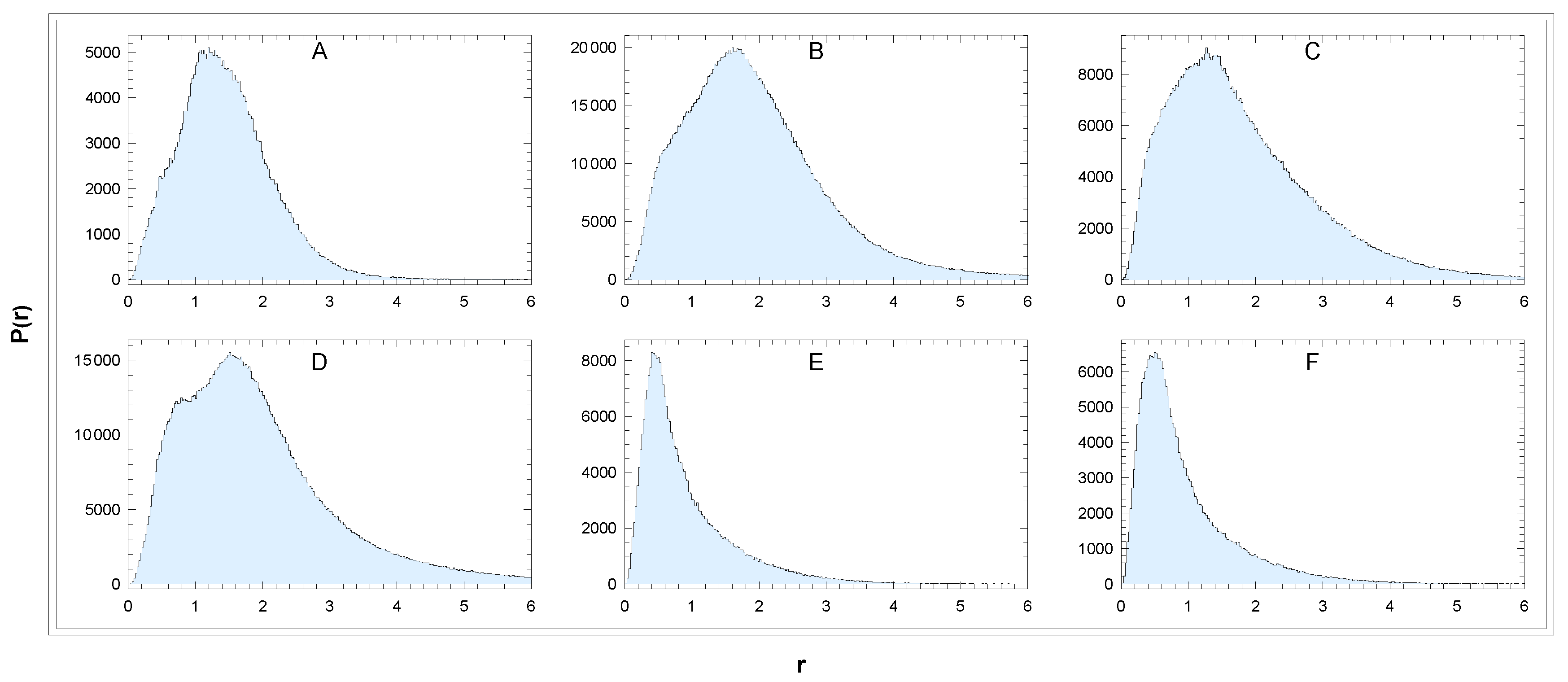
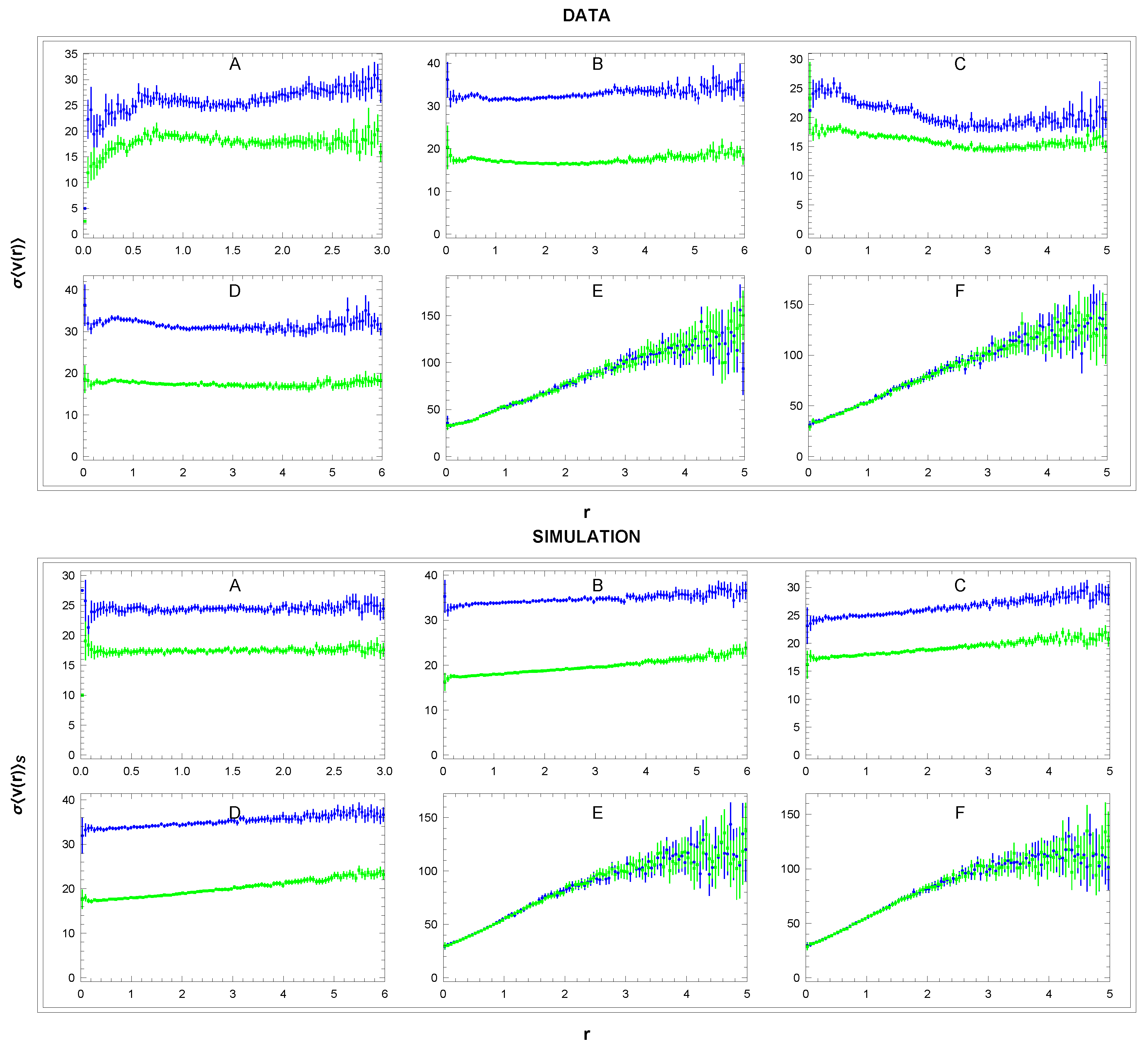
Figure 3.
Distribution of distances in the sectors A-F. Unit: r[kpc]. Binning: 0.024kpc.
3.1. Velocity of the Sun
According to (
8) and (
15) the Sun’s velocity can be decomposed as
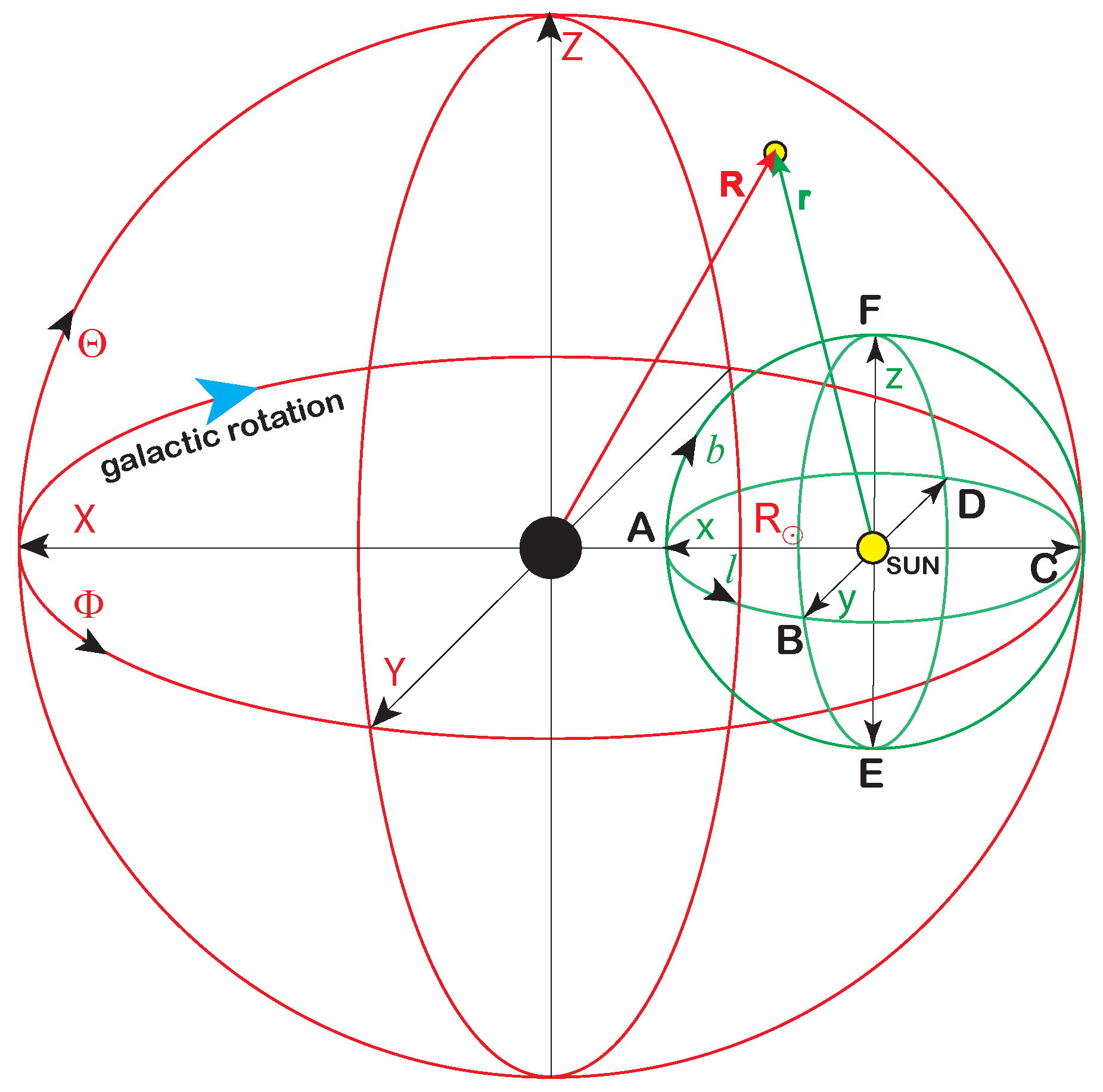
where
is the LSR velocity and
is the Sun’s velocity in the LSR frame. How can these velocities be determined? In the galactic reference frame the star velocity
is given as
which implies
The region of averaging
should be reasonably wide to suppress the influence of local fluctuations on the obtained average, then the first two terms cancel and for the local Sun’s velocity we obtain
For its calculation, we use the projections of galactic velocities (
12) in sectors A-D shown in
Figure 4 together with the relations
where the vectors of local orthonormal basis
are defined in (7). In the sectors considered, we get:
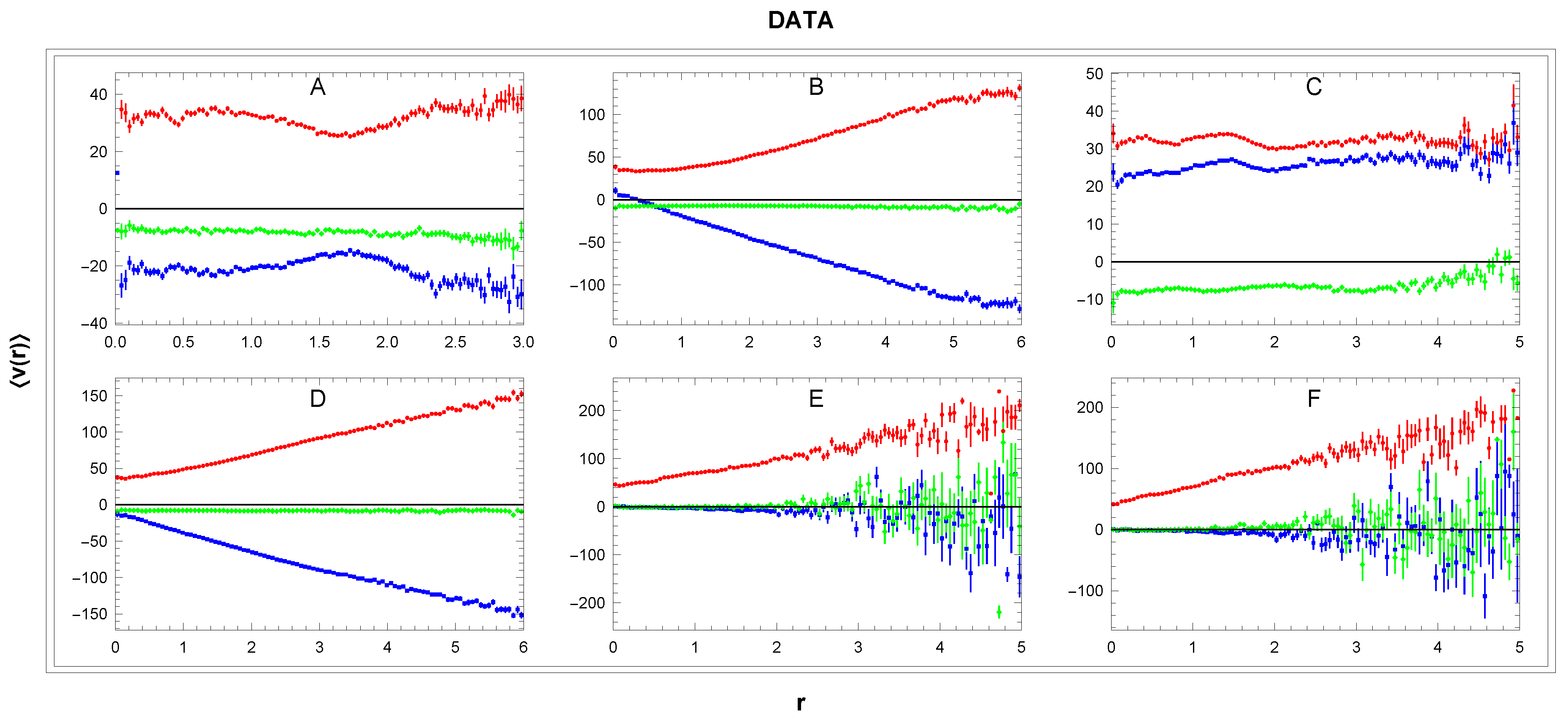
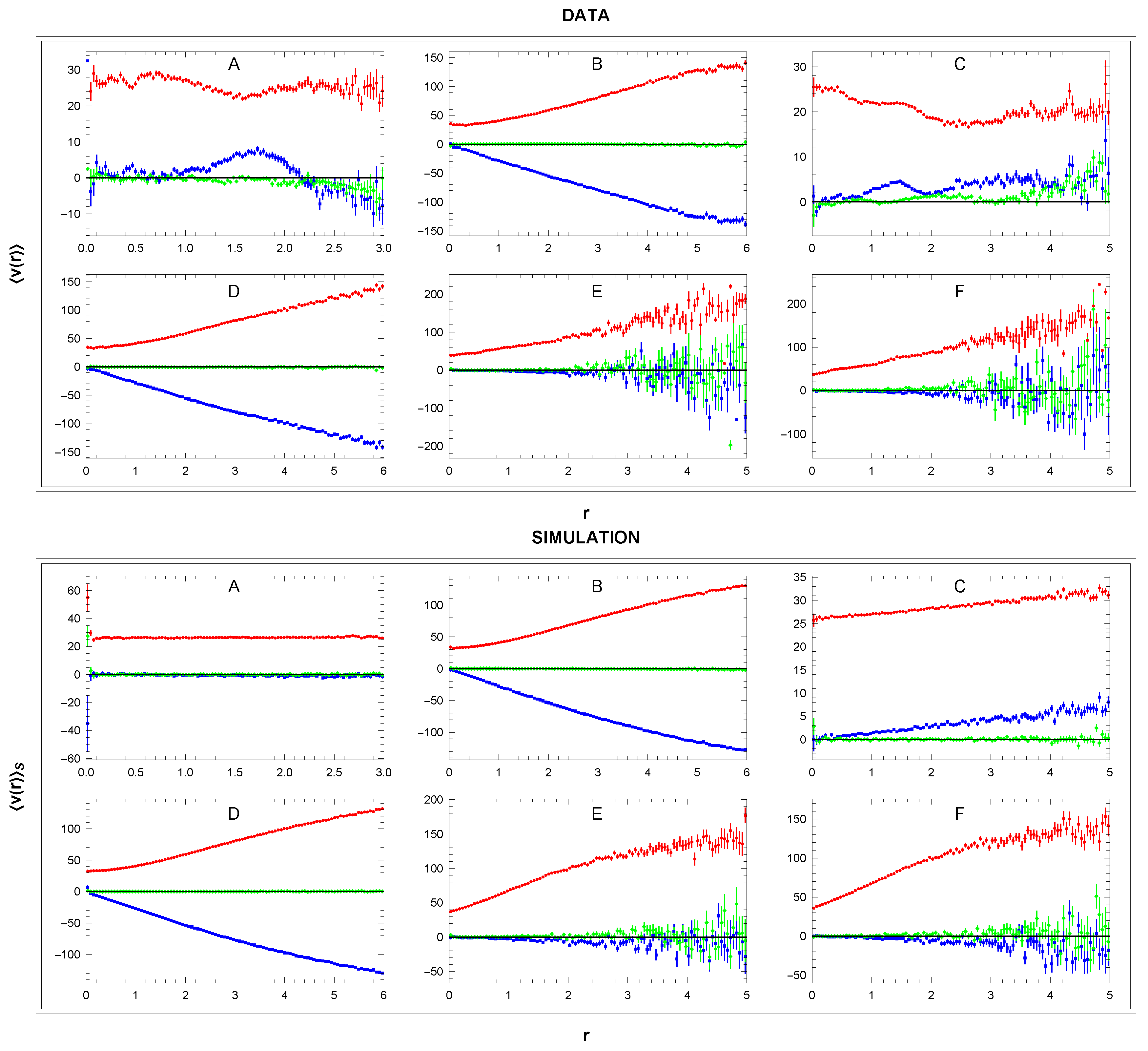
Figure 4.
Dependence of mean velocity ( - blue, - green, - red) on distance r in the galactic reference frame in sectors A-F. Cut . Units: r[kpc], v[km/s].
Figure 4.
Dependence of mean velocity ( - blue, - green, - red) on distance r in the galactic reference frame in sectors A-F. Cut . Units: r[kpc], v[km/s].
1)
in the sectors A-D Since in these sectors we have
so we can identify
. The mean values
depending on distance
r are for individual sectors shown in
Figure 4. The velocity
is the average
where
means the region of averaging, which are the stars in the sectors A-D and radius
. The resulting curve is shown in
Figure 5.
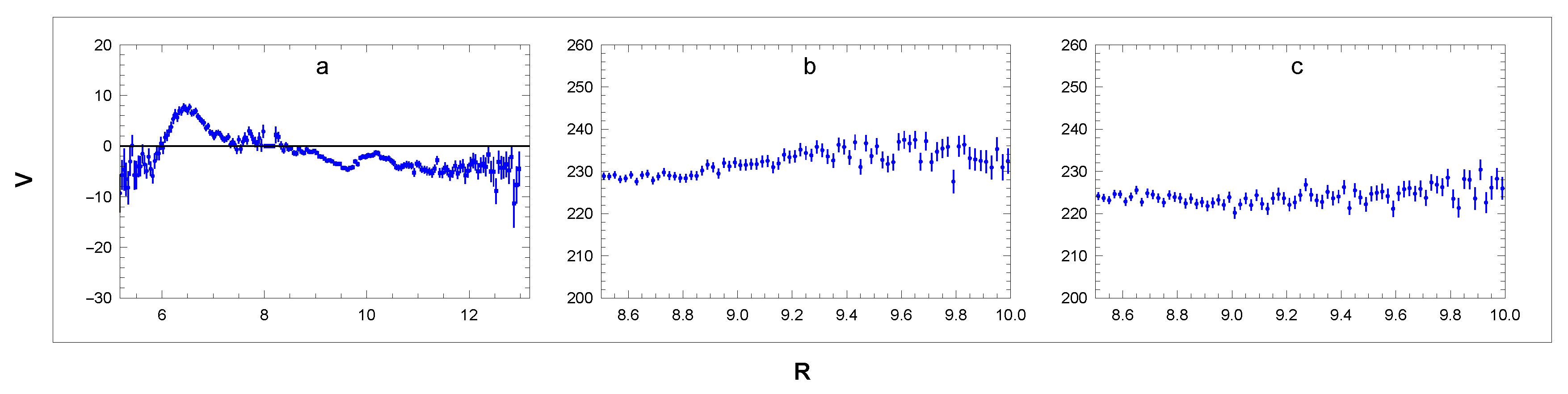
Figure 5.
Velocities (blue) and (green) as the functions of (left) with corresponding statistical errors (right). Cut . Units: [kpc], [km/s].
Figure 5.
Velocities (blue) and (green) as the functions of (left) with corresponding statistical errors (right). Cut . Units: [kpc], [km/s].
2)
in the sectors A and C In these sectors we have
, so we identify
in the A and
in the C sector. The corresponding curves
are in panels A,C (
Figure 4) and curve
is in
Figure 5. The region of averaging are sectors A and C up to the distance
3)
and
in the sectors B and D Here we have
so we can identify
in the sector B and
in the D sector. In panels B,D in
Figure 4 we show corresponding
curves. For small
r we have
, which implies for B,D sectors
but what is the reason for the steep slope of
as
r increases? In the considered sectors, the mean value
includes a significant contribution from the collective rotation velocity
proportional to
r, as explained below (
Figure 9 and Eq.(
43)). Thus, in B,D sectors we have
and correspondingly
The two curves
are shown in
Figure 6 together with the curve produced by fitting the free parameters
and
in the range
kpc. Assuming that rotation velocity is constant in these sectors,
, we obtain very good agreement of the fit to the data. In the next we abbreviate
by
. The obtained velocities are:
Admittedly, there is a weak dependency [
18,
39]
however the range
kpc means that
, which is too small a range for reliable fit involving
.
Figure 6.
Curves (
29): data (
blue) and fit (
red). Cut
. Units: r[kpc],
[km/s].
Figure 6.
Curves (
29): data (
blue) and fit (
red). Cut
. Units: r[kpc],
[km/s].
In the left panel of
Figure 5 we observe nearly constant curves, while the right panel shows dependence of corresponding statistical errors. The range of distances
involves the dominant part of analyzed stars in sectors A-D. To estimate the Sun’s local velocity
, we take the values in the middle of the range
. The velocities
and
are obtained as averages of the values in (
30).
However, for consistent comparison with other analyses, the velocities
and
can require further correction based on the calculation of asymmetric drift (see [
14], Sec.11):
where
is the MW circular velocity at
and
is a mean orbital velocity of the stars in neigborhood of the Sun. The Sun orbital velocity
in the Galactocentric frame can be decomposed alternatively as
so
The study [
49] estimates the asymmetric drift
around the Sun’s position to be about 6 km/s. A very similar value can be extracted from
Figure 3 in the paper [
40], where the parameter
is replaced by our parameter
km
2s
−2, which is calculated in
Section 3.3, (
Table 4). In the standard notation, we can identify
where
and
are the averages of the corresponding values in (
30). We have:
The associated velocities
and
are shown in
Table 3.
Table 3.
Local velocity of the Sun, mean rotation velocity and circular velocity along with the results of other analyses. Units: [km/s].
Table 3.
Local velocity of the Sun, mean rotation velocity and circular velocity along with the results of other analyses. Units: [km/s].
|
|
|
|
|
|
|
ref. |
|
|
|
228 |
234 |
|
|
this work |
|
|
|
|
|
|
|
[40] |
|
|
|
|
|
|
|
[11] |
|
|
|
|
|
|
|
[43] |
|
|
|
|
|
|
|
[17] |
| |
|
|
|
|
|
|
[39] |
| |
|
|
|
|
|
|
[12] |
|
|
|
|
|
|
|
[32] |
| |
|
|
|
|
|
|
[28] |
|
|
|
|
|
|
|
[18] |
| |
|
|
|
|
|
|
[13] |
| |
|
|
|
|
|
|
[41] |
| |
|
|
|
|
|
|
[37] |
| |
|
|
|
|
|
|
[20] |
| |
|
|
|
|
|
|
[33] |
| |
|
|
|
|
|
|
[48] |
| |
|
|
|
|
|
|
[26] |
| |
|
|
|
|
|
|
[27] |
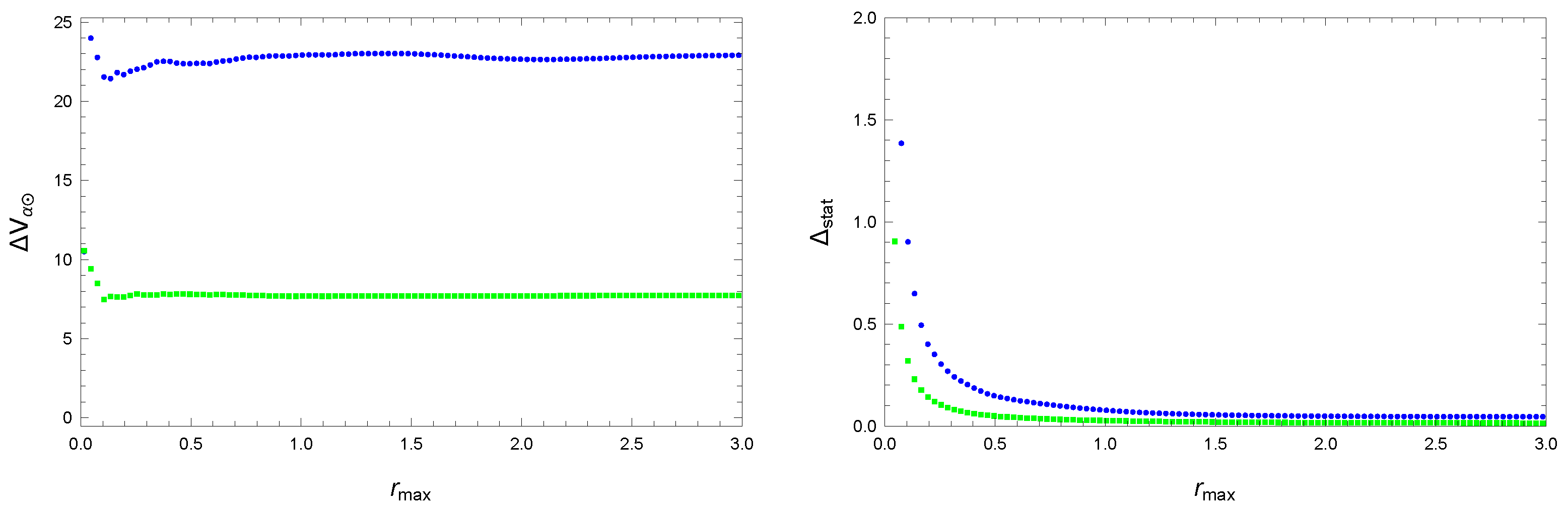
Their systematic uncertainties are estimated as follows. For velocities are defined by the range of variability of the curves in the left panel in interval kpc. For velocities and systematic uncertainty is estimated from a set of fits in different intervals of distances . The relatively small systematic uncertainty in reflects the relatively small local variations.
3.2. Rotation Curves
From now, we will substitute galactic velocity
in (
21) by
, which is the velocity related to the LSR:
In this frame, the input data (
12) are modified with the use of our
as
After this substitution,
Figure 4 is replaced by the top panel in
Figure 7.
Figure 7.
Dependence of mean velocity (
- blue,
- green,
- red) on distance
r in the local rest frame at
in sectors A-F. For panel DATA we used cut
. For panel SIMULATION see
Section 3.3 and
Section 3.4. Units: r[kpc], v[km/s].
Figure 7.
Dependence of mean velocity (
- blue,
- green,
- red) on distance
r in the local rest frame at
in sectors A-F. For panel DATA we used cut
. For panel SIMULATION see
Section 3.3 and
Section 3.4. Units: r[kpc], v[km/s].
The new
refer to the LSR whose velocity is
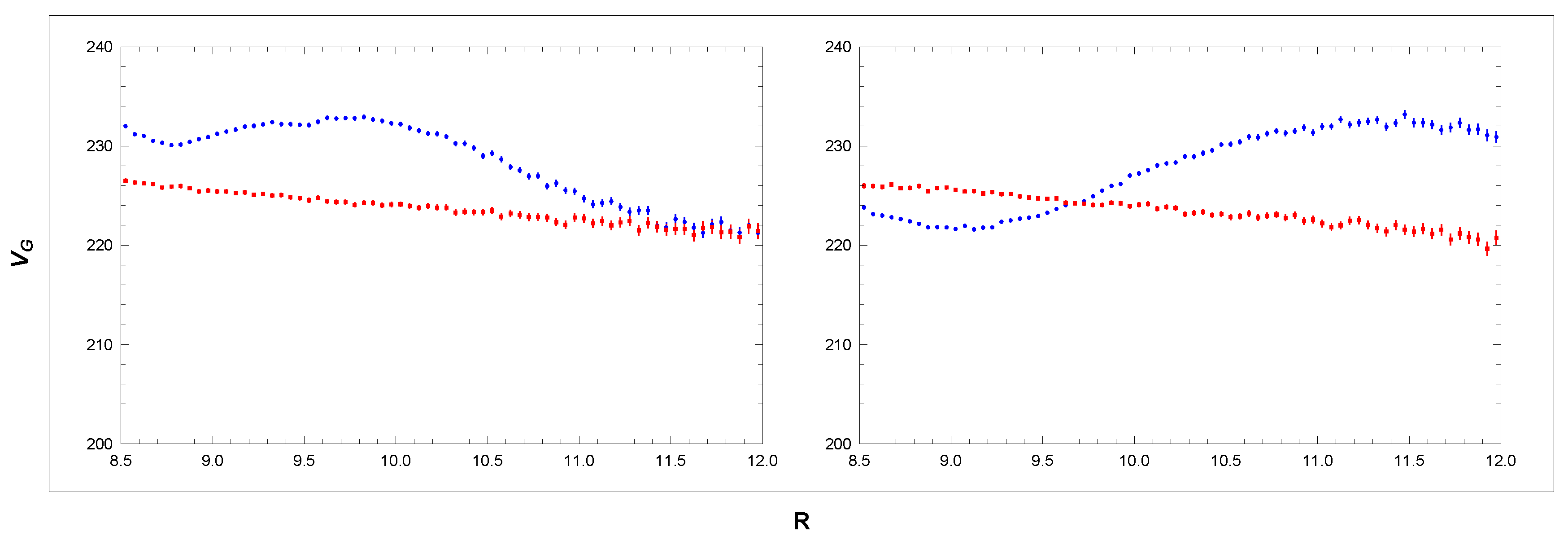
The combination of the new panels A and C, which represents the RC is shown in
Figure 8a.
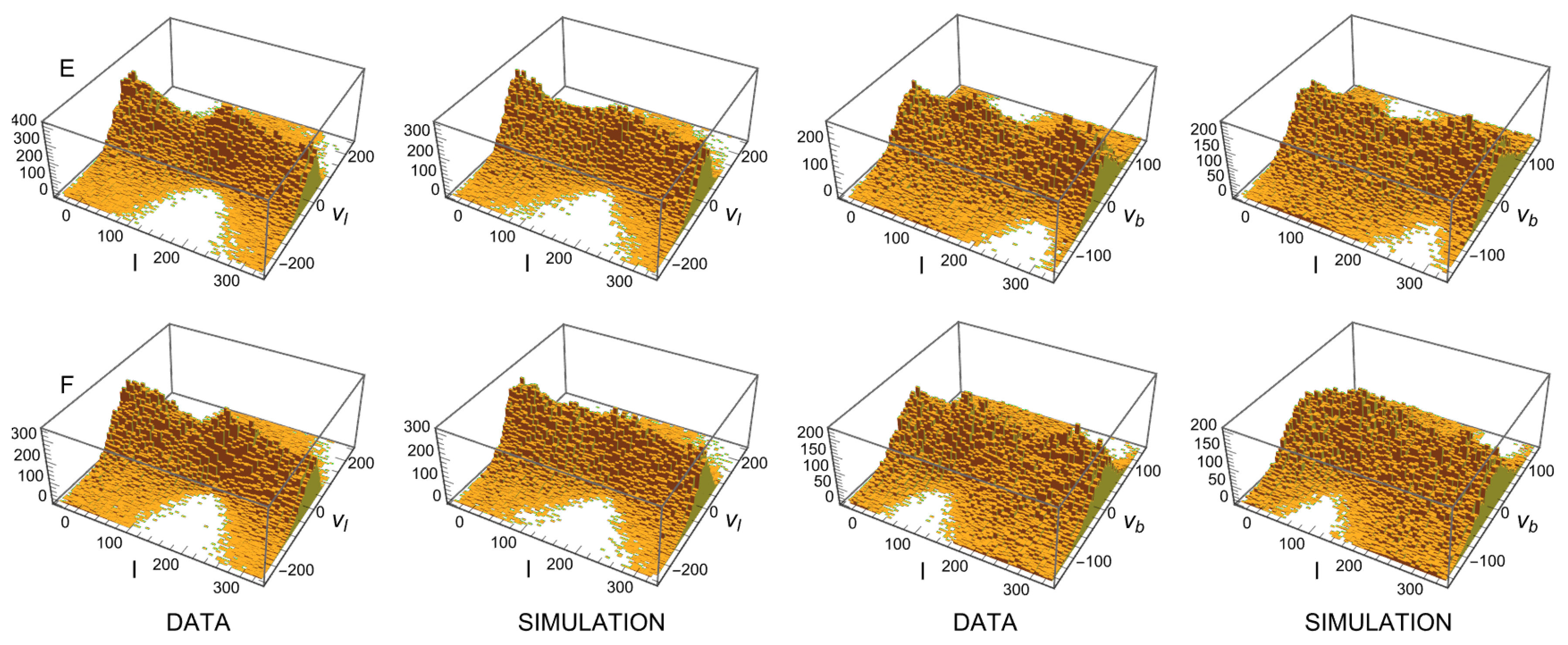
Figure 8.
Velocity curves in sectors A+C (panel (a)) and in sectors B and D (panels (b) and (c)). For panel (a) we used cut . Units: R[kpc], v[km/s].
Figure 8.
Velocity curves in sectors A+C (panel (a)) and in sectors B and D (panels (b) and (c)). For panel (a) we used cut . Units: R[kpc], v[km/s].
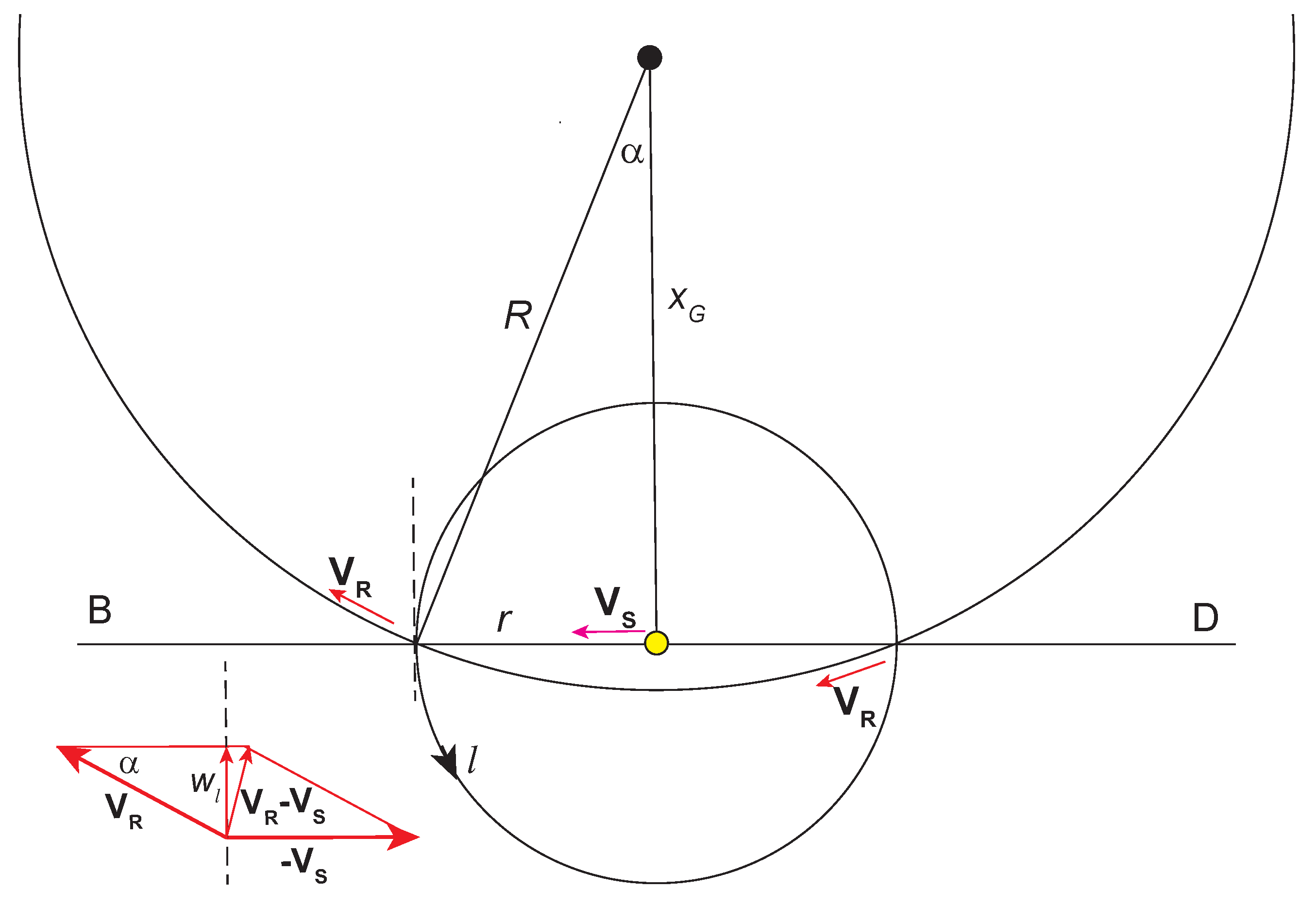
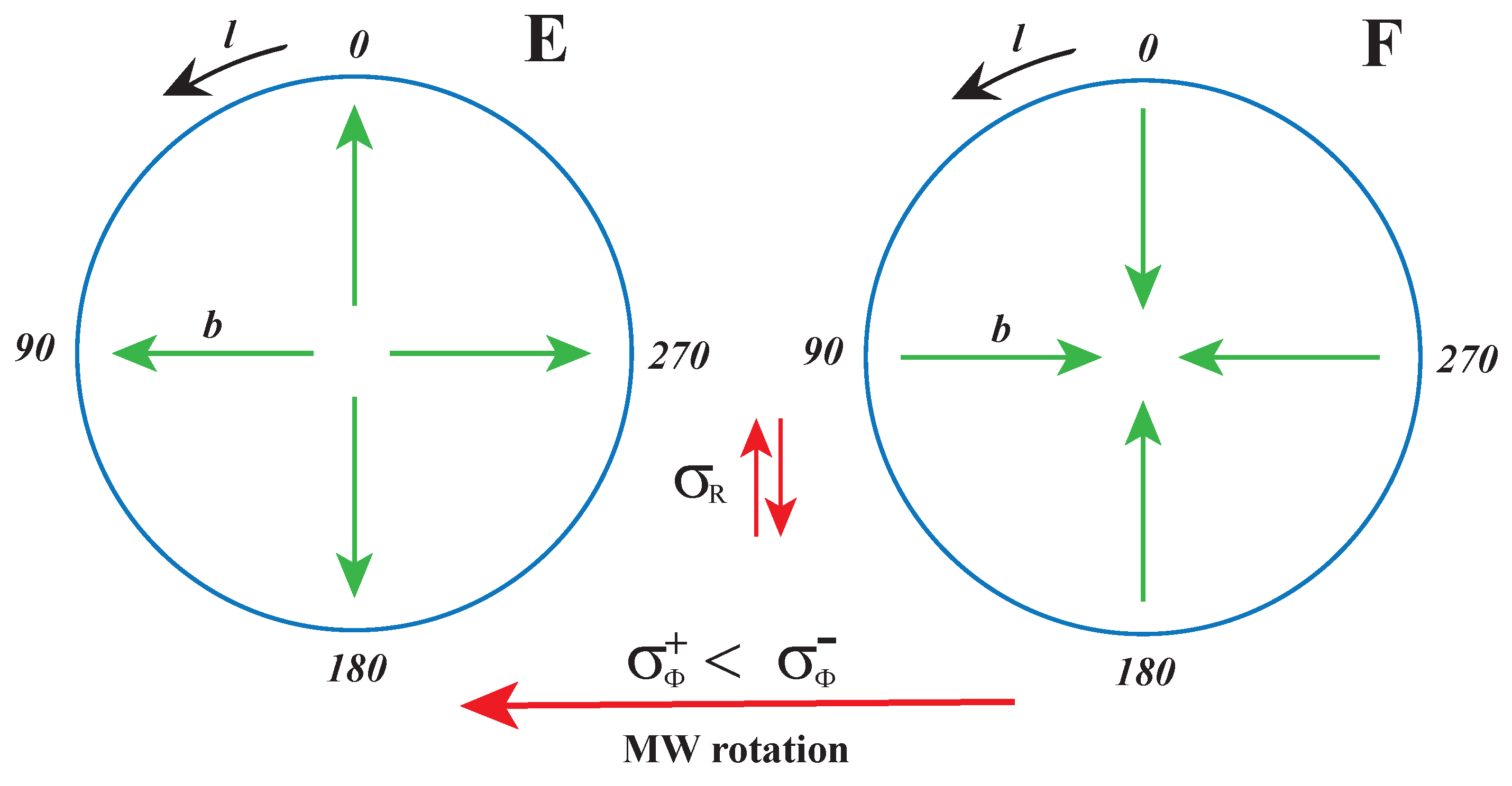
Figure 9.
Rotation of MW as seen in sectors B and D. Here the symbols and stand for and
Figure 9.
Rotation of MW as seen in sectors B and D. Here the symbols and stand for and
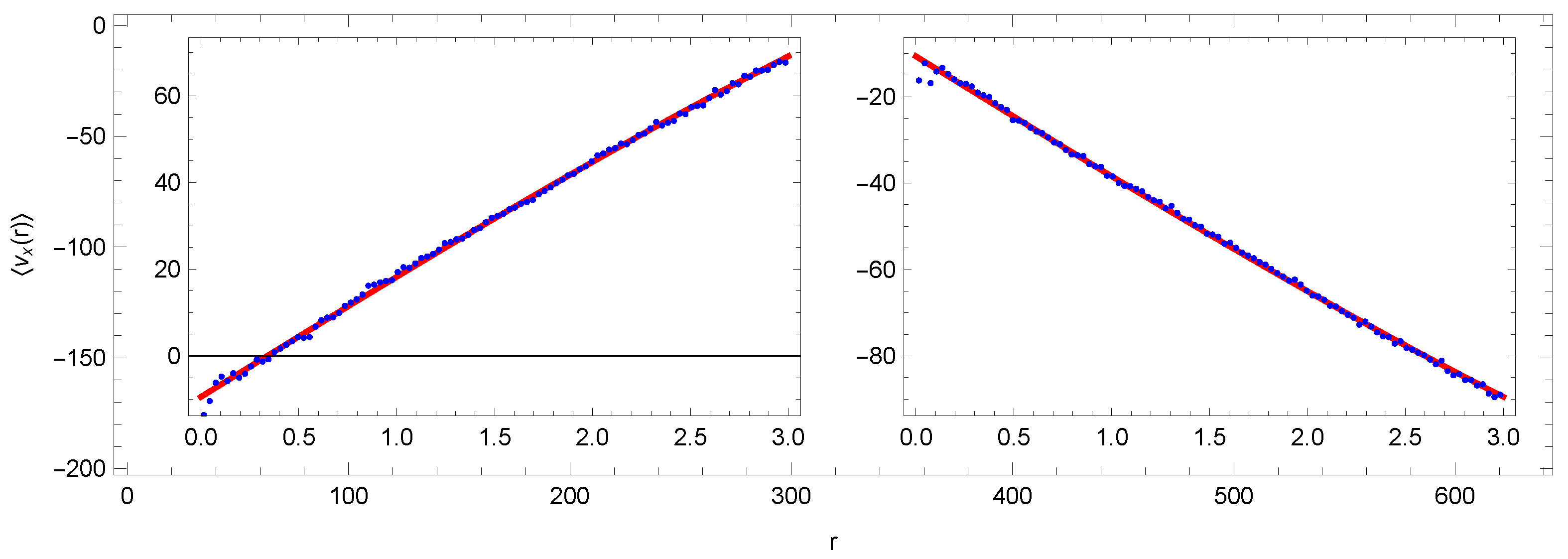
Another representation of the RC is obtained from panels B and D. For
and
the term
in Eq.(38) and its transverse projection
are calculated as suggested in
Figure 9 from two similar orthogonal triangles with angle
We obtain
Since
, we get
The corresponding RCs are shown in panels b,c of
Figure 8. These curves are a different representation of the
curves in panels B and D of
Figure 7.
Relation (
43) holds only for sectors B and D, where
and
(or
). In the general case, the geometry is more complicated. With the use of (
24) and (38) we have
This relation can be modified as
With the use of relations (
6),(
3) and (
1, vector
can be expressed in galactic coordinates
and after a few further modifications, we get
and if
, then
One can check that in sectors B and D, where
,
and where we have assumed
, relation (
47) reduces to (
43). Relation (
48) allows us to analyze
not only in narrow sectors B and D but also in the wider regions, which can provide higher statistics with smaller errors. This relation is not suitable for the reconstruction of
in the vicinity of singularity
. In
Figure 10
(blue points) we show RCs obtained with the use of (
48) in the sectors Q
2 and Q
4. In the analyzed area we observe irregular fluctuations in the rotation velocity:
. The relation allows us to calculate rotation velocity not only in the galactic plane, but also outside the plane. In
Figure 11
we show the velocity curves calculated in sectors and .
3.3. Six Parameters of the MW Collective Rotation
Panels E and F at the top of
Figure 7 provide further important information. We observe
and
, as expected in both narrow cones pointing perpendicularly from the galactic plane, where positive and negative
are equally abundant. On the other hand, the value
increases with distance from the plane. This increase occurs in the galactic reference frame reflecting the slowing of collective rotation in the Galactocentric frame, which increases with
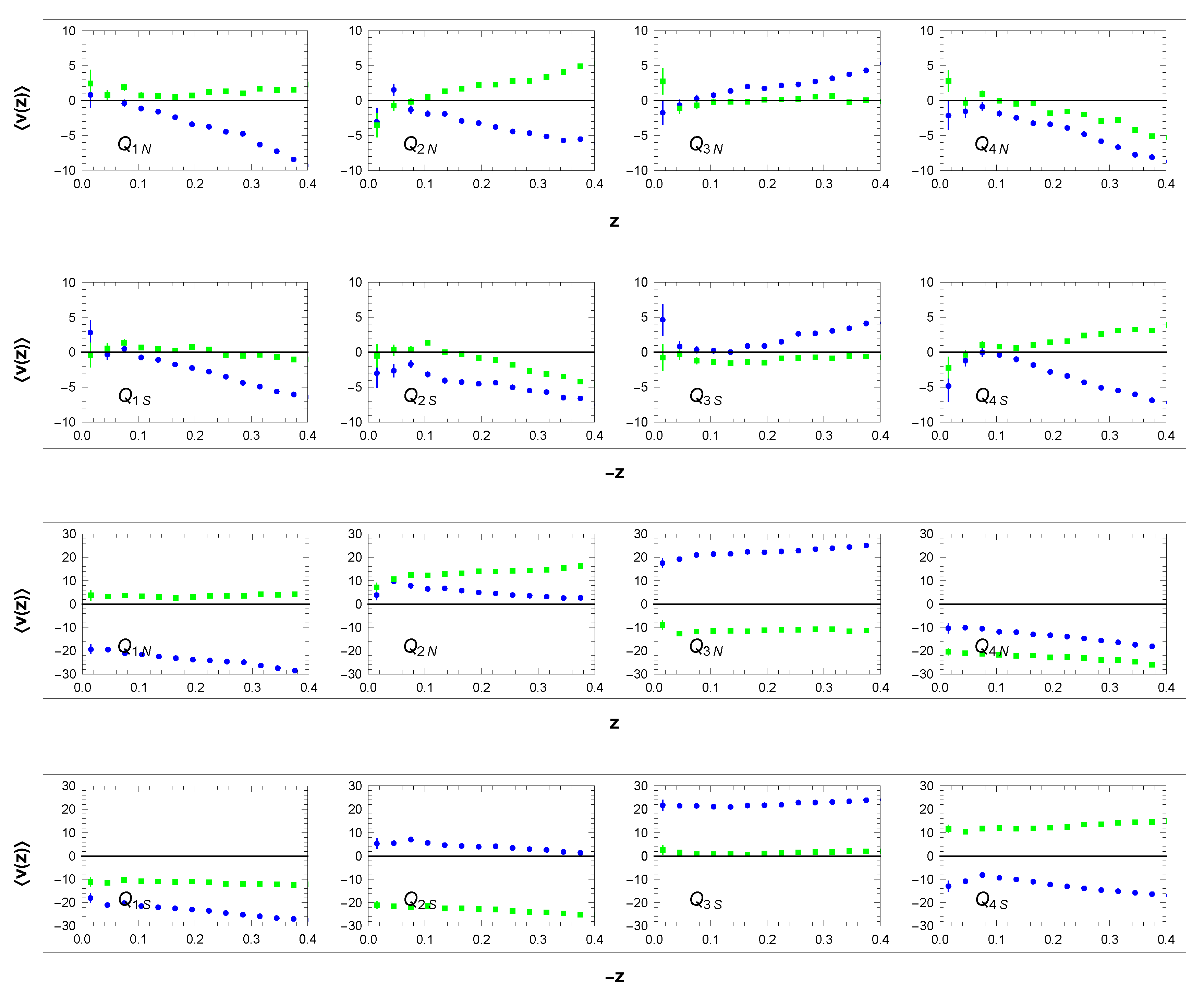
. The same effect is seen even more clearly in
Figure 11. Important information is obtained from
Figure 12,
where dependencies of standard deviations are shown. The increasing standard deviations in panels E and F suggest a less collective, but more disorderly motion of high velocities away from the galactic plane.
In the distribution (
16), we assume in a first approximation:
where
and
are the free parameters. We proceed as follows in their setting:
i) From the data panels A-D in
Figure 12 where
, we estimate
In directions other than A-D, the relations between
’s in the galactic and Galactocentric frames are more complex. The data panels E and F (where
), show in the region of the peaks (
kpc, see
Figure 3, panels E,F) a linear increase of the corresponding mixture of
’s with
.
ii) To obtain the parameters
, we analyzed the respective distributions in all the sectors listed in
Table 1. We found that the optimal shape of the distribution
in (
16) is asymmetric, having different
for the two opposite orientations, where
means
in (against) the rotation direction:
Thus, only
depends on
. This asymmetry also reflects the effective deceleration
of the collective rotation for larger
as mentioned above. We have
After integration we get
The parameter
is obtained by the fit from
Figure 11, which suggests dependence
For the remaining two parameters, the analysis showed that
is a good approximation. We denote
, this last free parameter was set up from the tuning of the slope in simulation panels E and F in
Figure 12. A list of the six resulting parameters controlling simulation (
16) is given in
Table 4.
Table 4.
Monte-Carlo simulation model parameters and corresponding parameters from other analyses. Velocity
is taken from
Table 3.
Table 4.
Monte-Carlo simulation model parameters and corresponding parameters from other analyses. Velocity
is taken from
Table 3.
|
|
|
|
|
|
ref. |
| 17 |
24 |
33 |
20 |
42 |
228 |
this work |
|
|
|
x |
x |
x |
[2] |
| 11 |
20 |
31 |
x |
x |
x |
[45] |
The relation (
56) shows that the MW rotation at
kpc is
km/s lower than at
, which is significantly less than the total error in determining
. Therefore, we have neglected
in our calculation. The Wolfram Mathematica code of the generator is available on the website
https://www.fzu.cz/~piska/Catalogue/genkinFEB24.nb.
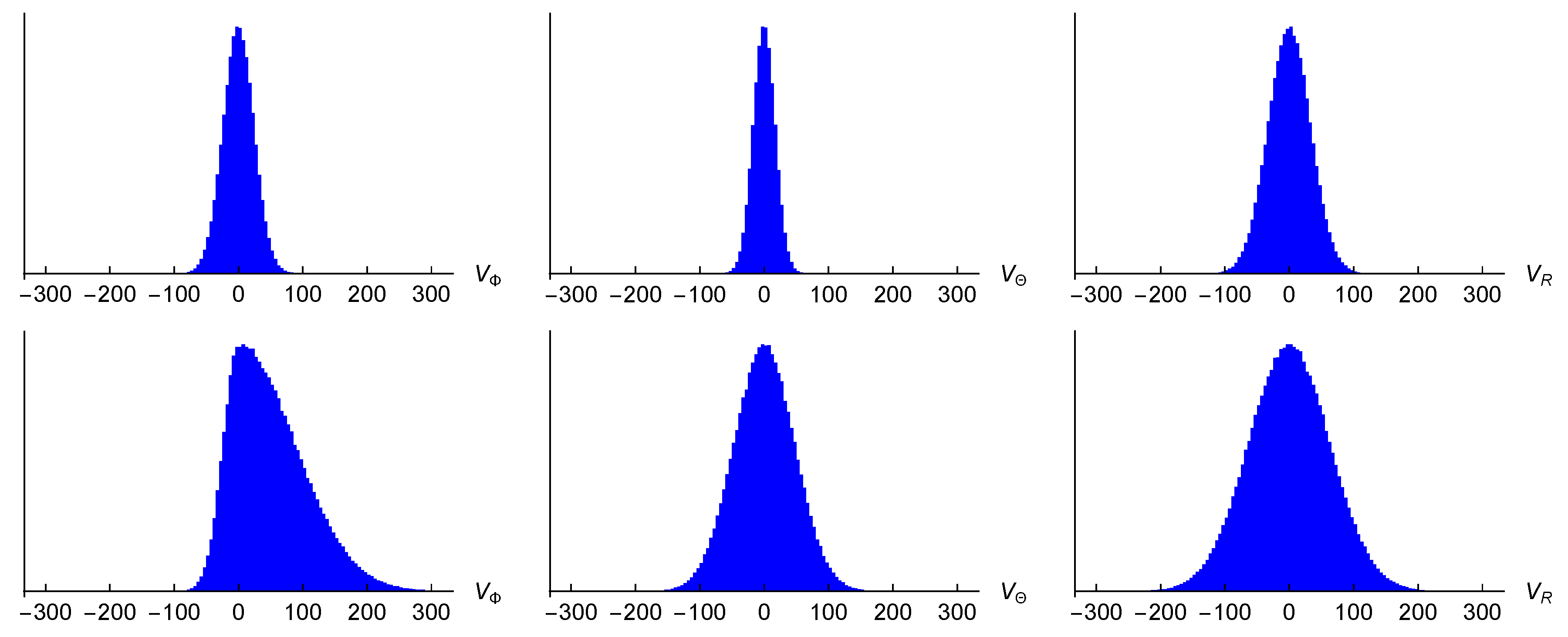
Figure 13
shows the examples of the distribution of simulated velocities and . The simulated distributions and are symmetric for any , distribution is asymmetric for .
3.4. Comparison of Simulation Model with Data
The comparison is done as follows:
1) Position
of the source in the galactic reference frame is with the use of Eqs.
3 transformed to the Galactocentric spherical frame
. For this position, the velocity
defined by (
14) is generated according to distribution (
16) with the parameters from
Table 4.
2) Using (
41) and (7) we get the corresponding LSR transverse velocities:
So for any source defined by input
we generate a vector
and then create the desired distributions from both.
3) These distributions obtained from the input data and simulations will now be compared. The comparison in
Figure 7 shows perfect agreement between data and simulation for panels B,D,E,F. In panels A and C, the simulation model does not reproduce local kinematic substructures generating deviations
km/s. The presence of these substructures shows the precision with which we work. At the same time, the fluctuations are not noticeable in the other panels because their velocity scale is coarser.
The simulation in panel C indicates that the velocity increases with r, despite the constant parameter . This small effect is because we are working inside the angle deg, which means a slight linear increase in average and correspondingly some deceleration with r. So, a corresponding correction would therefore be necessary to evaluate the RC in this sector more accurately. We have checked that for smaller angles this effect disappears. At the same time, we do not observe a similar effect in sector A. The reason is that in a very dense field of this sector our cuts and accept only a narrow sector of the data: deg.
Figure 12 shows the corresponding velocity dispersion dependencies. In the upper panels A-D we again observe fluctuations that are not present in the simulation. In panels E,F with a coarser scale the fluctuations are not noticeable. Averaged data in panels A-D were together with panels E,F used to determine parameters
in
Table 4. After averaging the fluctuations the simulation model fits the data well.
Relatively small velocity fluctuations (
km/s,
) also appear in the RC in
Figure 10. The slightly decreasing simulated RC is due to the shape of the sectors
and
, where a larger
R correlates with a larger average
, implying smaller
.
Figure 11 shows that the simulation of decreasing
controlled by the fitted parameter
in Eq.(
56) agrees well with the data.
The good agreement of the simulations with the data is confirmed by other results.
Figure 14.
Distributions of and in sectors A-F: data and simulation model. Unit: v[km/s]. Binning: 1.6 km/s.
Figure 14.
Distributions of and in sectors A-F: data and simulation model. Unit: v[km/s]. Binning: 1.6 km/s.
Figure 15.
Histograms and in sectors E and F: data and simulation.Units: l[deg], v[km/s]. Binning : deg km/s km/s.
Figure 15.
Histograms and in sectors E and F: data and simulation.Units: l[deg], v[km/s]. Binning : deg km/s km/s.
Figure 16.
Asymmetry
in the Galactocentric reference frame generates asymmetries in the galactic frame, see text and
Figure 15.
Figure 16.
Asymmetry
in the Galactocentric reference frame generates asymmetries in the galactic frame, see text and
Figure 15.
Figure 17.
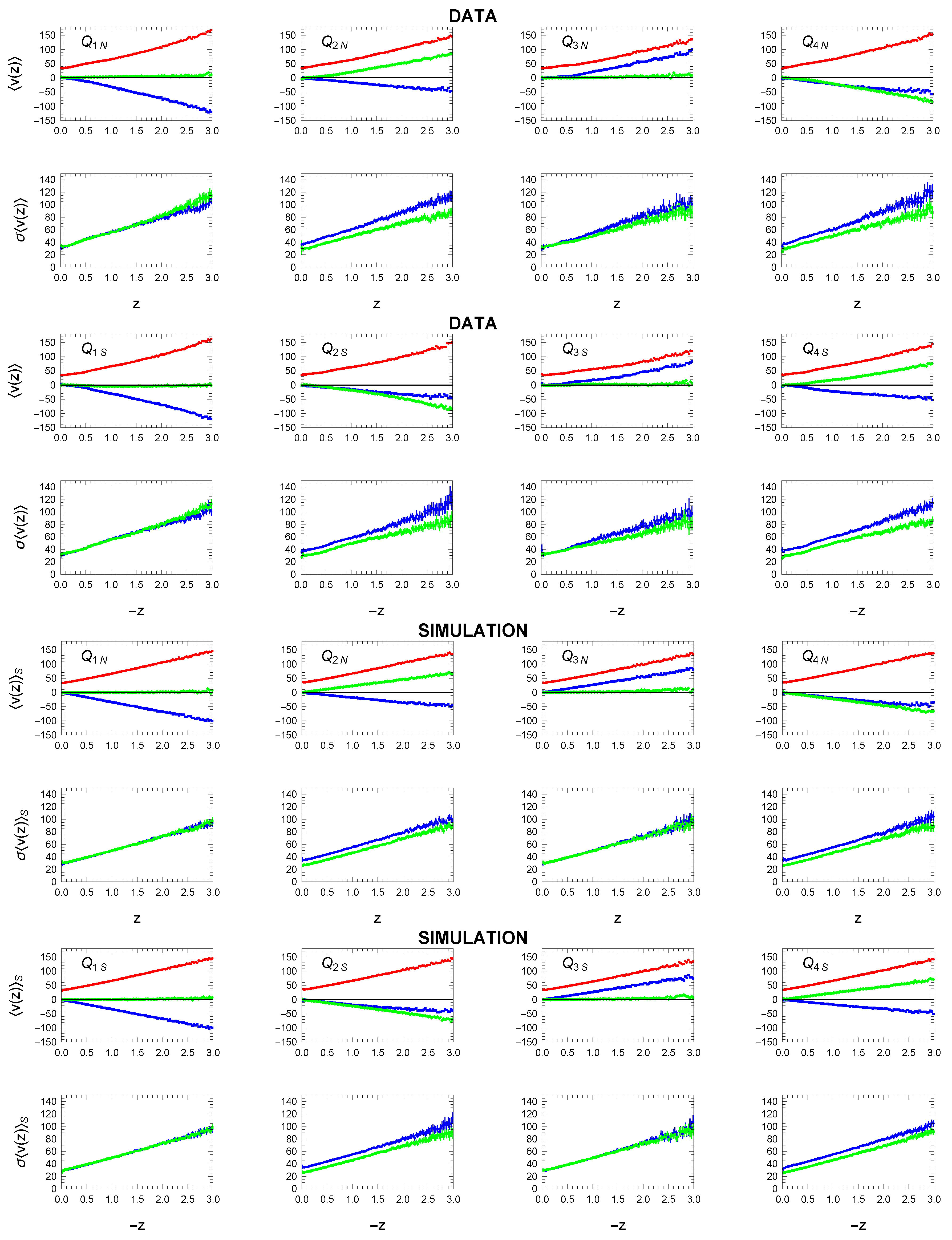
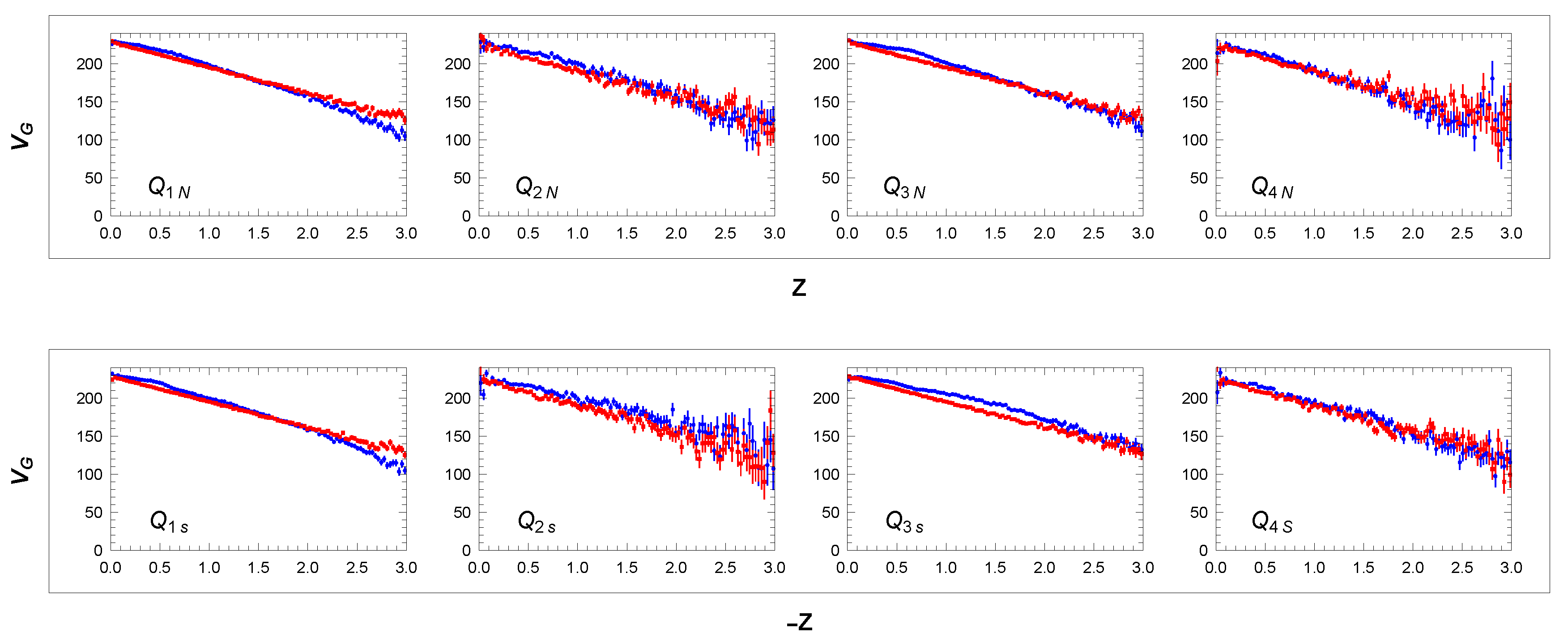
Dependence of mean velocity and its dispersion ( - blue, - green, - red) on distance z in sectors - and -: data and simulation model. Units: z[kpc], v[km/s].
Figure 17.
Dependence of mean velocity and its dispersion ( - blue, - green, - red) on distance z in sectors - and -: data and simulation model. Units: z[kpc], v[km/s].
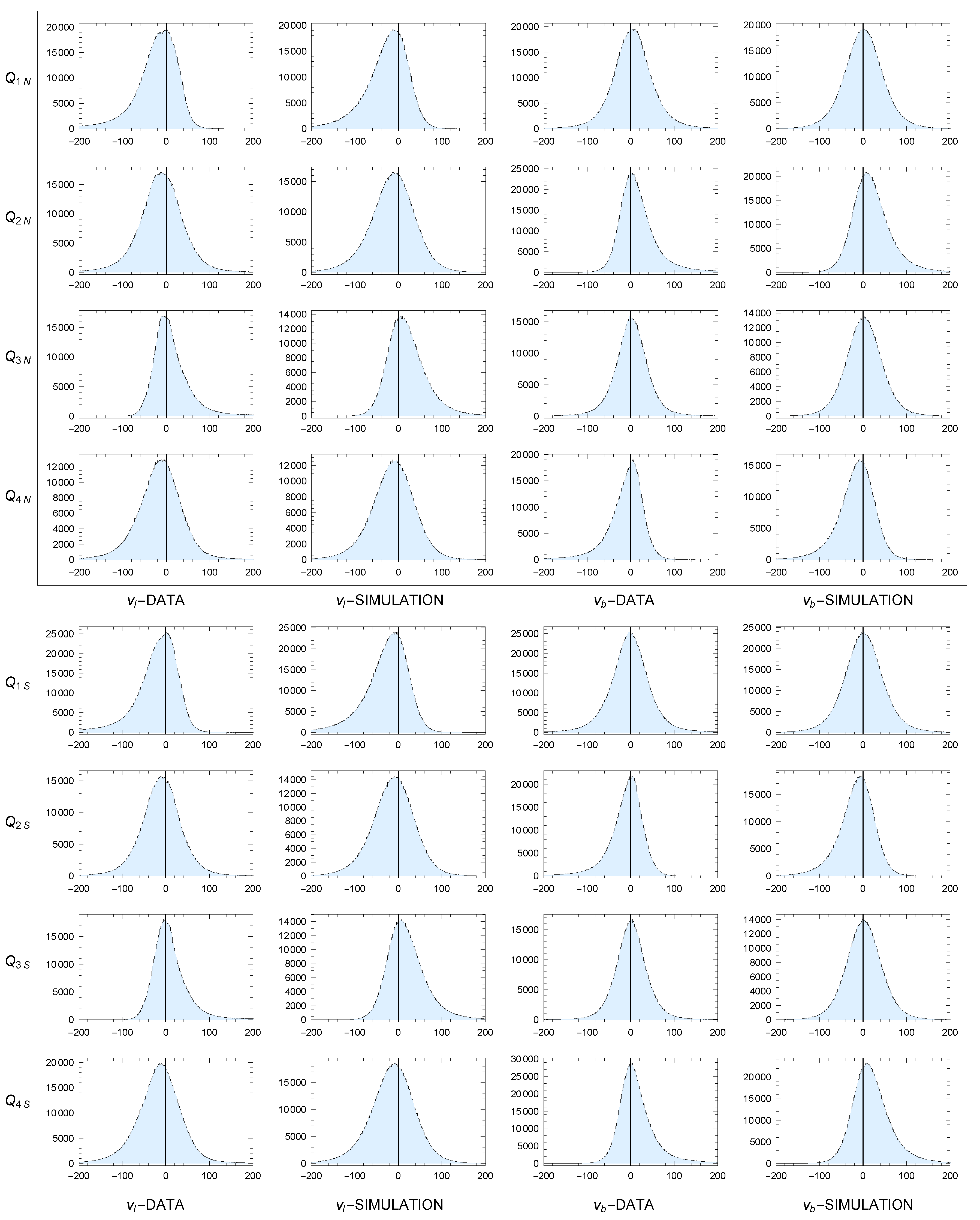
Figure 18.
Distributions of and in sectors , : data and simulation model. Unit: v[km/s]. Binning: 1.6 km/s.
Figure 18.
Distributions of and in sectors , : data and simulation model. Unit: v[km/s]. Binning: 1.6 km/s.
Table 5.
Correspondence of dispersions
of velocity distributions of
and
at
in sectors E,F with velocity dispersions in the Galactocentric reference frame
and
The origin of the asymmetries is suggested in
Figure 16.
Table 5.
Correspondence of dispersions
of velocity distributions of
and
at
in sectors E,F with velocity dispersions in the Galactocentric reference frame
and
The origin of the asymmetries is suggested in
Figure 16.
| sector∖l[deg] |
0 |
90 |
180 |
270 |
| E,F |
|
|
|
|
| E |
|
|
|
|
| F |
|
|
|
|
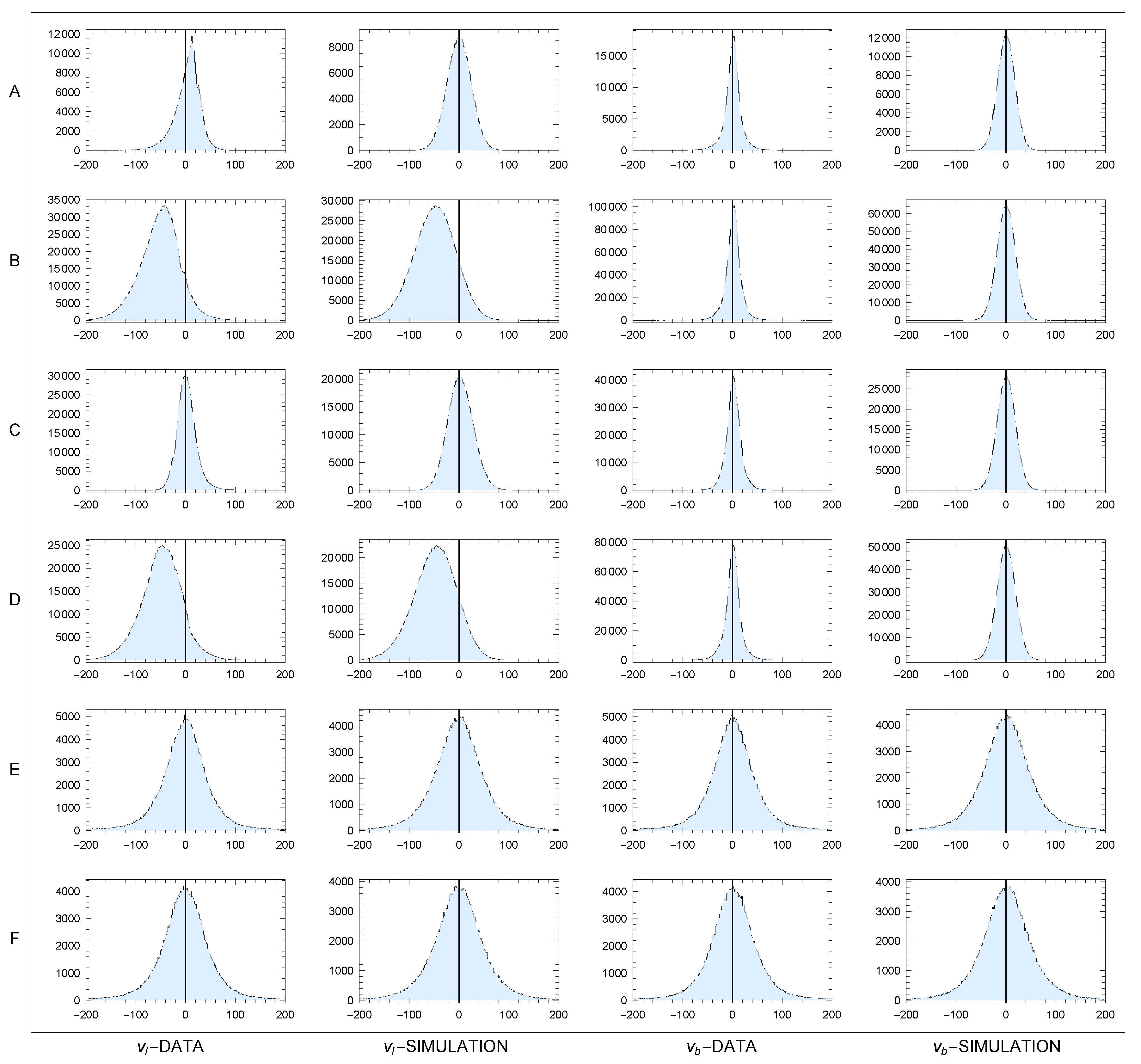
Figure 14 shows distributions of
and
in sectors A-F along with the corresponding distributions obtained from simulations. In sectors A-D we observe a narrower distribution of
, the width of which does not depend on the sector. The distributions have roughly the same dispersion for both data and simulation, but the peak in the data is sharper. The peaks in the data also have slightly longer tails, which increase the dispersion. The simulated shape is therefore only approximate. The distributions of
are slightly different. Note the shift in sectors B and D resulting from the decrease in
in upper panels B and D in
Figure 7. The distribution
DATA in sector A (where
) also has a sharper peak with an apparent asymmetry. This may be a manifestation of the asymmetric drift effect. So the simulated shape is only approximate here as well. In the opposite sector C (where
), the asymmetry is negligible. The distributions of
in both sectors A and C are copies (up to a constant shift) of the distribution of orbital velocities in the Galactocentric frame.
The important result is shown in
Figure 15. The asymmetry of histograms
and
in sectors E and F with the empty spaces reflects different projections of the asymmetry (
53). The shape of histograms can be explained using
Figure 16 and
Table 5. Distributions of
for
are controled by the parameters
in the first row of table. Their connection with
and
can be deduced from figure. At
the directions of
and MW rotation are identical, so
. But at
, the two directions are opposite, so
. At
the situation is a little more complicated. If
or
are small (which is almost our case, see panels E,F in
Figure 3, where
r), then the
direction can be approximated by vector
, so
. Similarly for
distributions controlled by
in the next rows of the table. Histograms involve integrated distributions over sectors E and F. Also here, the agreement between the data and simulation model is perfect.
Correct Monte-Carlo parameter settings can be verified in wide Q-sectors outside the area of the galactic plane.
Figure 17 shows
dependence of mean values and dispersions of velocity distributions in these sectors. The curves together with the corresponding overall distributions of velocities in broad sectors
,
in
Figure 18 again confirm the perfect agreement of the simulation with data. Note in particular the projections
in sectors
,
,
,
and
in sectors
,
,
,
. This is also due to the asymmetry (
53) that occurs for
, as illustrated by simulated
distribution in
Figure 13.