Submitted:
25 November 2024
Posted:
26 November 2024
Read the latest preprint version here
Abstract
A cascade control structure (CCS) is still the most commonly used control scheme in variable speed control (VSC) electrical drives with AC motors. Several tuning methods are used to select the coefficients of controllers applied in CCS. These approaches can be divided into analytical, empirical, and heuristic ones. Regardless of the tuning method used, there is still a question of whether the CCS is tuned optimally in terms of considered performance indicators to provide high-performance behavior of the electrical drive. Recently, artificial intelligence-based methods, e.g., swarm-based metaheuristic algorithms (SBMA), have been extensively examined in this field, giving promising results. Moreover, the intensive development of AI assistants based on large language models (LLMs) supporting decision-making processes is observed. Therefore, it is worth examining the ability of LLMs to tune the CCS in the VSC electrical drive. This paper investigates tuning methods for the cascade control structure equipped with PI-type current and angular velocity controllers for PMSM drive. Sets of CCS parameters from electrical engineers with different experiences are compared with reference solutions obtained by using the SBMA approach and LLMs. The novel LLM-based Tuning Assistant (TA) is developed and trained to improve the quality of responses. The obtained results are assessed regarding the drive performance, number of attempts, and time required to accomplish the considered task. The results indicate that AI-based tuning methods and the properly trained Tuning Assistant can significantly improve the performance of VSC electrical drives, while state-of-the-art LLMs do not guarantee high-performance drive operation.
Keywords:
cascade control structure
; variable speed drive
; permanent magnet synchronous motor
; tuning assistant
; artificial intelligence
; large language models
1. Introduction
Variable speed drives (VSDs) with permanent magnet synchronous motors are commonly applied in high-performance industry applications such as robotics, CNC machines, and recently in electromobility and aircraft [1,2,3,4,5,6]. It is caused by superior dynamic properties, reliability, and energy efficiency of considered motors [7,8,9]. Full use of the listed features requires precise information about drive signals and an accurate control scheme. The actual values of the motor’s phase currents and the shaft angular position can be obtained using encoders and Hall-effect current sensors. To improve the VSD level of safety, estimation techniques and fault detection mechanisms are introduced [10,11,12,13,14].
PMSM, as a typical AC motor, is described by electrical and mechanical equations with different dynamic properties. Therefore, control schemes can be divided into two main groups: (i) cascade control structure (CCS) with the inner and the outer control loops, and (ii) cascade-free with a complex control scheme. The second approach, implemented as a state feedback control, provides robustness against parameter variations and better disturbance compensation compared to CCS [8,15,16]. However, its tuning process is relatively complex and usually requires expert knowledge. Recently, SBMA has been applied in this field, and these show superior properties in comparison to the analytical approach [15,16]. It should be pointed out that SBMA is based on the optimization of the performance function, and the overall drive performance is strongly related to its components. Therefore, expert knowledge and experience are required during the performance function construction and SBMA parameters selection [17,18].
Contrary to the cascade-free complex control scheme, the CCS is based on a series of connections of well-known PID controllers. In this approach, controllers are tuned separately, and several tuning methods can be used. These can be divided into three main groups: (i) empirical, (ii) analytical, and (iii) computer-aided. In the first group, the controller coefficients are usually selected by trial and error or using Ziegler-Nichols-like approaches. The overall drive performance and the time needed to accomplish the tuning procedure are strongly related to user experience and may result in non-optimal behavior [19,20]. From the literature review, it can be seen that mistakes that disable correct drive operation are common, even for a basic control structure. In [21], negative values of the PI speed controller are enabled, which may result in positive feedback and loss of stability. From the results shown in [22], one can see that improper controller tuning may result in a huge overshoot and poor load torque compensation. Instead of applying a proper tuning procedure, the authors suggest the introduction of low-pass filters or non-linear control law.
The analytical approach utilizes a symmetric optimum criterion for the angular velocity controller and a magnitude optimum criterion or an internal model control (IMC) theory for the current controller [23,24]. These approaches require more advanced knowledge from electrical drives and control theory compared to the empirical solutions listed above and, therefore, are commonly applied by more advanced electrical engineers. In [25], the IMC is combined with model following control to provide velocity control of PMSM with reduced impact of the load torque. The authors report that the presented control structure is much more insensitive to disturbances at the plant input compared to the classical cascade control structure. On the other hand, an explicit tuning procedure for the controller, which generates an additional control signal responsible for load torque compensation, is not precisely defined. It was also mentioned that the proposed solution is based on model knowledge, and modeling a complex plant, e.g., a CNC control system, can be a challenging task. An optimized PI tuning scheme based on an analytical approach, namely deadbeat predictive conception, is proposed in [26]. It was found that the integration gains in both controllers are equal to zero, and therefore, the load torque observer must be applied to provide steady-state error-free operation of the drive. The formulas proposed for proportional gains of both controllers are simpler compared to the reference solutions but in the angular velocity controller, a manually selected coefficient is present. As the authors reported, its value should be chosen during experimental tests.
As in the case of complex control schemes, the tuning process of PI controllers in a cascade control structure can also be supported by AI-based approaches. In [17,18], several SBMAs are applied to adjust the parameters of the velocity PI controller in the PMSM drive. The objective function responsible for setting the maximum overshoot and the rise time and elimination of the steady-state error has been proposed. The weighting factor has also been introduced to shape the dynamic properties of the control system. Based on the simulation results, it was concluded that the velocity controller is tuned properly, and the drive tracks the given trajectories well, including the load torque compensation. A similar conclusion can be found in [27], where a comparison between a conventional PI speed controller tuned by using the Ziegler-Nichols approach and one using the optimization scheme (i.e., multivariable sliding-mode extremum seeking) is shown. Faster attainment of steady-state, reduced overshoot, and enhanced robustness against load torque and parameter variations were reported. However, the user must select additional parameters responsible for the drive’s dynamic behavior and smooth control action. As in the case of a cascade-free control scheme, the final behavior of the drive with SBMA-tuned controllers strongly depends on the performance function applied, and therefore expert knowledge is required in this area.
The intensive development of large language models causes their area of application to expand [28]. Recently, the ability of LLM to solve undergraduate control engineering problems has been examined using the state-of-the-art LLM’s: GPT-4, Claude 3 Opus, and Gemini 1.0 Ultra [29]. It was reported that answers generated by LLMs are sometimes inconsistent even for the same problem, and the reasoning and calculation capabilities must be improved in the future. In [30], the innovative combination of an adaptive PID controller with an LLM to enhance explainability was proposed. The potential of LLMs to bolster the control loop performance has been demonstrated. As an example, the integration of the GPT-3.5-turbo into the control loop of a convoy of autonomous vehicles was shown in a simulation study.
In this paper, a novel Tuning Assistant based on the large language model is proposed and examined. A data set necessary to accurately train the TA is described, and a two-stage training process is presented. The developed solution is used to find the coefficients of PI-type angular velocity and current controllers for a variable speed drive with a permanent magnet synchronous motor. The obtained results are compared with reference solutions, namely answers from the state-of-the-art LLMs, responses from electrical engineers, and outturns from swarm-based metaheuristic algorithms. The innovative use of LLM in tuning the cascade control structure allows the drive to obtain superior control behavior.
This paper is organized as follows. Section 2 introduces the mathematical description and methods for the determination of the main parameters of the PMSM. The description of a cascade control structure and tuning methods used in PMSM drives are also included in this section. Section 3 explores the results obtained from the Tuning Assistant. These are compared with reference solutions, namely the state-of-the-art LLMs, swarm-based metaheuristic algorithms, and finally, responses from electrical engineers. In Section 4, the obtained results and discussed. Here, conclusions and the potential directions for future research are also outlined.
2. Materials and Methods
2.1. Determination of the Parameters of the PMSM
Analytical methods used to determine coefficients of PI current and velocity controllers are based on the knowledge of the drive’s parameters. These can be obtained using measurements, as shown in [31], or identification described in [32]. In the later part of this section, the calculation of the motor’s electrical and mechanical parameters will be discussed.
2.1.1. Electrical Parameters of the Motor
The electrical part of the PMSM can be described using the following formulas, usually written in reference frame:
where , are space vector components of voltages, , are current space vector components, is angular velocity, , are stator resistance and inductance, p is the number of pole pairs, is flux linkage. From (1)-(2), one can see that precise control of the PMSM currents requires knowledge of the stator resistance and inductance. These can be calculated from the motor’s electrical circuit step response parameters under the assumption that the motor shaft is locked, resulting elimination of the back-emf components. The motor’s resistance can be computed from the steady-state value of the step response:
where is the steady-state value of the commanded voltage, and is the steady-state value of the current, as shown in Figure 1.
Next, the motor’s inductance can be calculated from the obtained time constant:
where is the electrical time constant estimated from the current step response presented above. To improve the accuracy of calculations, the experiment should be conducted for different values of the commanded voltage, and the motor’s shaft should be immobilized. It may also be necessary to take into account the converter gain. In such a case, the steady-state value of the commanded voltage in (1) will be multiplied accordingly [33].
2.1.2. Mechanical Parameters of the Motor
The mechanical part of the PMSM can be described using the following equation:
where and are the motor’s moment of inertia and the viscous friction coefficient, is the torque constant, and is the load torque. From (5), it can be seen that accurate control of the PMSM angular velocity depends on the knowledge of the motor’s mechanical parameters, namely , , and . These can be calculated from the motor’s response parameters if they are unknown. In such a case, it is necessary to command the step values of the reference current and record the angular velocity waveform in the current/torque mode of the drive. The gain coefficient of the mechanical part can be calculated from the following formula:
where is the steady-state value of the angular velocity. Next, the object’s moment of inertia can be computed from the following formula:
where is the mechanical time constant estimated from the velocity step response, as shown in Figure 2.
Now, it is also possible to estimate the viscous coefficient of the mechanical part of the object using the following formula:
Further information related to the identification of motor parameters can be found in [32].
2.2. Cascade Control Structure
As stated before, the cascade control structure (CCS) with the inner and the outer control loops is considered in this study. The choice is related to the behavior of the electrical drive, where different dynamic properties are observed for electrical and mechanical parts, as well as to the well-known structure and tuning methods of PI controllers. The selection procedures of the controller’s coefficients will be discussed in the later part of this section, while the considered CCS is shown in Figure 3.
From Figure 3, it can be seen that a standard or textbook version of the PI controller is utilized. In the case of the outer angular velocity controller, is the proportional gain of the controller, while is the integration time constant of the controller. Similarly, in the inner current control loop, is the proportional gain of the controller, while is the integration time constant of the controller. The controller from the outer control loop generates a reference signal for the inner control loop, i.e., , while the controller from the inner control loop generates a control signal for the modulator [33]. Since nonlinear limitations exist in electrical drives (e.g., limited voltage of the voltage source inverter, limited current, and angular velocity of the PMSM), it may happen that the control variable reaches the actuator limits. In such a case, the error will continue to be integrated by the integral path of the controller, resulting in deterioration of the control performance [34]. To overcome this drawback, the tracking back-calculation method can be implemented to attenuate the integral path during saturation [33]. As shown in Figure 3, the tracking time constants and (i.e., anti-windup coefficients) are used in the anti-windup path. These determine how quickly the integral is reset.
In the case of the other controller’s structure, the coefficients should be converted before implementation, as shown in [35]. For example [33], instead of the integration time constant , the gain can be utilized. A similar modification can be found for the tracking time constant implemented as the gain . Here, the subscript x will be replaced by i for current controllers, while for the angular velocity control loop, it is substituted by .
2.3. Tuning Approaches
In this part, the tuning methods of the control structure described previously will be discussed. Typically, these can be divided into two main groups: (i) analytical-based tuning and (ii) empirical-based tuning. Recently, it was found that AI-based approaches can successfully support the tuning process, both analytical- and empirical-based methods. All of these will be discussed later in this section.
2.3.1. Analytical-Based Tuning
In this approach, it is necessary to maintain the tuning order of the controllers, i.e., from the inner (current) to the outer (angular velocity) control loop. In the case of the current control loop tuning, it should first be decided whether the current overshoot is permissible. Since the magnitude optimum criterion presented in [23] provides a fast current response and slight overshoot, these can be used to calculate the controller coefficients analytically. In this case, the dominant time constant in the plant (i.e., ) is canceled by the zero in the controller, resulting in the following formulas for PI current controller:
where is the switching frequency. If the current overshoot is not allowed, the internal model control (IMC) approach presented in [24] can be used to calculate the coefficients of the PI current controller. Here, the parameters of the controller are expressed directly in machine parameters and the desired rise time of the control loop. Such an approach simplifies the design procedure by reducing the trial-and-error steps. According to the IMC approach, the PI current controller’s coefficients will be as follows:
It is worth pointing out that regardless of the method used, the same formula is proposed for the calculation of the integration time constant. In IMC, a suitable trade-off between the current control loop’s bandwidth and the current signal’s noise can be obtained [33]. The current rise time is typically specified as a couple of control periods [36].
In the next step, the angular velocity controller will be designed. Here, the symmetric optimum criteria can be used [23]. It is necessary to know the object’s moment of inertia, the torque constant of the motor, and the time constant of the current control loop. The PI velocity controller’s coefficients will be as follows:
where is the time constant of the current control loop. As stated in [23], there will be a 43% overshoot if the abovementioned coefficients are used. To improve the control system’s velocity transient response (i.e., reduction of an overshoot), an input filter of reference velocity may be introduced. It is positioned outside the loop without affecting the load torque compensation. As a result, an 8.1% overshoot can be obtained.
The controller’s coefficients obtained using (9)-(10) or (11)-(12) and (13)-(14) should be treated as initial ones. The discretization period from the drive should also be considered during the implementation of the integration time constant. If the control performance needs to be further improved, consider adjusting the anti-windup [34] and/or anti-resonance filters according to the drive documentation. To quickly reset the integrator, a very small value of the tracking time constant should be chosen. As shown in [34], the initial value of this anti-windup coefficient can typically be in the range of .
2.3.2. Swarm-Based Tuning
In this approach, computational intelligence is employed to find the optimal coefficients of the controllers. An application of swarm-based metaheuristic algorithms in tuning tasks has recently been observed. It is caused by better convergence and robustness against local minima compared to the exact optimization methods [37]. Contrary to the analytical-based solutions described above, here, all coefficients of the cascade control structure shown in Figure 3 are determined simultaneously. As shown in [37], several SBMAs can be used to solve the tuning task, and the choice may be related to the user experience and/or specific requirements. Regardless of the metaheuristic algorithm used, the general principle of operation can be described by the flowchart shown in Figure 4.
In phase 1, the control parameters specified for an SBMA are set, the population is initialized randomly, and the performance index is calculated for all swarms. Next, a part of the population is employed to global searching for the solution in the defined solution space. The performance index is again calculated for all swarms, and the best solution is remembered. At this stage, the constraint handling method can be employed to abandon solutions that exceed limitations [16]. In phase 3, the rest of the population is sent to the neighborhood of the best solution to improve the result. In order to improve convergence and avoid stagnation in a local minimum, additional mechanisms based on randomly changing the locations of some particles in the solution space can be used [37]. Finally, the optimization process is finished when the condition defined by the stopping criterion is met.
As described before, the operation of SBMAs is based on the optimization of the performance function, and the overall drive performance is strongly related to its components. To provide the desired behavior of the drive, several requirements should be taken into account during the performance index construction. The main control objective for the considered PMSM drive is to assure steady-state error-free operation and good dynamics of the angular velocity for both the reference and the load torque and step changes. Secondary control objectives related to zero d-axis current and chattering-free control signals can also be taken into account if high-performance drive operation is expected. The abovementioned requirements lead to the construction of the following performance index:
where , , and are the weighting factors responsible for prioritizing the impact of the performance index components. It is also possible to directly control the selected parameters of the plant response (e.g., the rise time, the overshoot) during auto-tuning [17].
In this paper, the ABC optimization method was chosen to find the initial coefficients of the controllers shown in Figure 3. The choice of the ABC is based on the confirmed convergence and repeatability of results obtained in similar tasks [15,16]. The control parameters of the optimization scheme and the results obtained are presented and discussed later in the paper.
2.3.3. LLM-Based Tuning
By reasoning, learning, and incorporating knowledge into pre-trained neural networks, Large Language Models are changing human-machine interactions and improving work in many areas [38]. The natural language generation and question-answering abilities are also very desirable advantages in search engines and intelligent customer services [28]. The abovementioned properties make it advisable to verify the usefulness of LLMs in the controller’s tuning task.
With this approach, it was decided that the Tuning Assistant (TA) based on LLM be developed and investigated. As a base of the proposed TA, the AI Assistant from Ordemio has been chosen due to the learning ability from multiple data sources, simple development process, no hallucinations, and no-cost operations (with restrictions) [39].
In the first stage, based on the authors’ experience, a data set was selected, and respective articles were loaded to the TA knowledge. Since the considered task is related to the tuning process of the angular velocity and current controllers for the PMSM drive, it was decided to load the paper where the magnitude optimum and the symmetric optimum criterion are described [23]. The work with the IMC approach was also included since this method can be successfully applied to current control [24]. To provide information about the PID controller’s structures, the paper [35] was introduced as an additional source. In this case, the URL was pointed directly to the open-access version of the article. Finally, the data set was augmented by two papers using the above-mentioned control methods in the PMSM drive [33,40]. The results obtained for the assistant trained using such a data set are discussed later in the paper.
In the second stage, the TA was re-trained to examine if the reasoning and answering abilities could be improved. Here, additional pre-processed information related to the tuning procedure and presented in Section 2.1 - Section 2.2 and in subSection 2.3.1 was used.
The Tuning Assistant trained in this way is used to support the selection of CCS coefficients, and the results are shown in the following section along with state-of-the-art LLMs, namely OpenAI ChatGPT and Microsoft Copilot. Developed Tuning Assistant is available at http://fizyka.umk.pl/~ttarczewski/ta.html.
3. Results
Tuning methods for the cascade control structure equipped with PI-type current and angular velocity controllers for the PMSM drive described in the previous section have been investigated. A group of electrical engineers with different experience levels were invited to tune a model of the PMSM drive. The main parameters of the PMSM drive used in the considered task are listed in Table A1. As the reference signal, the angular velocity step from 0 rad/s to 3 rad/s at 50 ms has been applied. To investigate the disturbance compensation ability, the load torque step variations were introduced. Its value is equal to 3 Nm in the time period 200 ÷ 400 ms and 0 Nm outside this period. The above-mentioned values were set as initial ones. However, it was found that the electrical engineers did not modify these during the tuning task. Model of the PMSM drive developed in Matlab/Simulink environment was shared with the user invited to accomplish tuning task.
Received sets of controller parameters along with additional explanations, including the drive performance (i.e., performance index), number of attempts, and time required to accomplish the considered task, were analyzed, and these are listed in Table 1. The following colors were used to indicate selected data: red for swarm-based tuning, green for analytical-based tuning, and blue for LLM-based tuning. These results were presented as waveforms and described in the later part of this section.
Figure 5.
Step responses of PMSM drive with cascade control structure tuned using swarm-based optimization algorithms: (a), (c), and (e) angular velocity, (b), (d), and (f) space vector current components.
Figure 5.
Step responses of PMSM drive with cascade control structure tuned using swarm-based optimization algorithms: (a), (c), and (e) angular velocity, (b), (d), and (f) space vector current components.
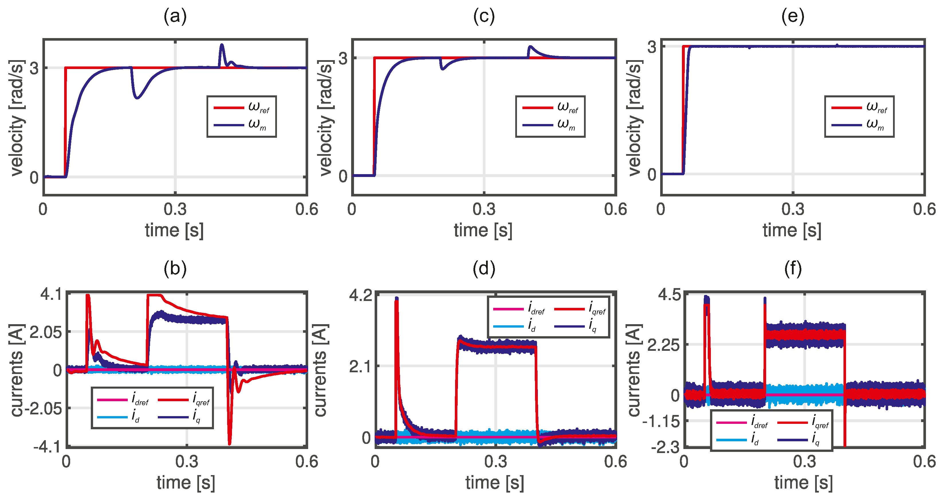
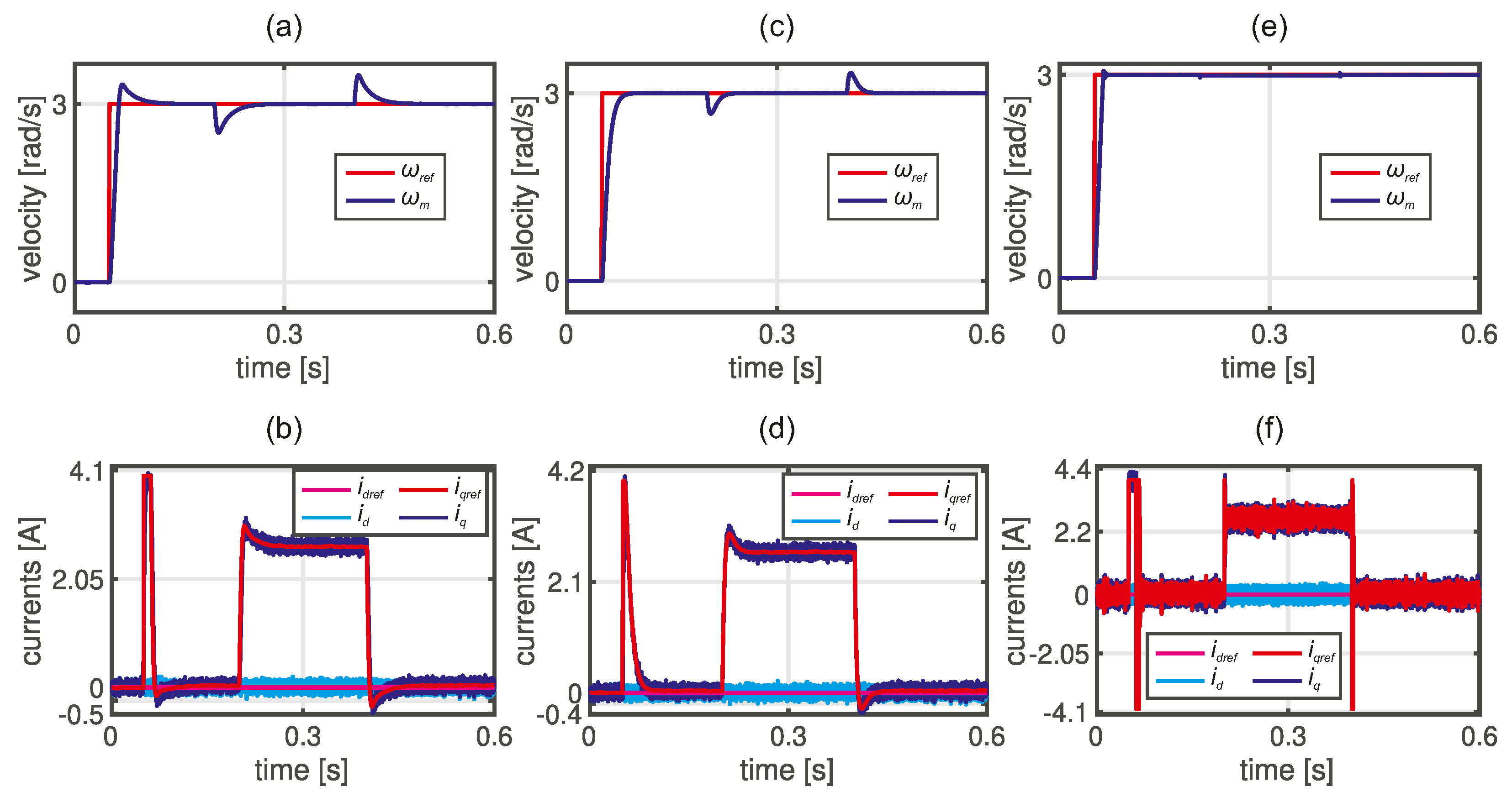
Figure 6.
Step responses of PMSM drive with cascade control structure tuned using analytical criteria: (a), (c), and (e) angular velocity, (b), (d), and (f) space vector current components.
Figure 6.
Step responses of PMSM drive with cascade control structure tuned using analytical criteria: (a), (c), and (e) angular velocity, (b), (d), and (f) space vector current components.
From the obtained results, it can be seen that the empirical approach is most often used together with auto-tuning. The mean value of the iteration number is equal to 116, and the mean time needed to accomplish the task is equal to 73 minutes. Significantly fewer iterations are observed if the empirical approach - the mean value of the iteration number equals 45. In such a case, the time required to tune the control structure is also shorter - the task lasts ca. 58 minutes. The highest number of iterations is obtained for SBMA’s, but this approach does not directly involve the users. Here, the task is accomplished in ca. 62 minutes, and the users reported that most of this time was spent on the integration of the drive’s model with the optimization procedure and developing the proper performance index to be optimized. Therefore, it is expected that another tuning attempt would take less time, as in the case of the solution from row 26 used as the initial set from auto-tuning by the users. The fastest responses related to the considered tuning task were received from LLMs. Copilot needs ca. 2 minutes, ChatGPT gives the responses after ca. 3 minutes, while the answer from TA powered by Ordemio came after ca. 1 minute. The conversation concerned tuning the current regulator, tuning the angular velocity controller, reducing possible overshoot, and selecting the anti-windup coefficient. The recording form conversations with LLMs is available to the reader as supplementary material attached to the paper.
It has been noted that there is a relationship between the chosen approach and the user experience. The empirical approach supported by auto-tuning is most often used by beginners. The advanced users rather prefer analytical methods but Ziegler-Nichols method-based approach with manual fine-tuning can also be found in the considered group. The swarm-based tuning came from advanced users only. Finally, it was found that beginner users mainly focus on minimizing the index, which leads to relatively large controller coefficients, which can lead to current oscillations in the transient and noisy operation of the drive. In the case of advanced users, a compromise between performance index minimization and secondary requirements related to signal oscillations is observed, resulting in relatively lower controller coefficients. Selected results from Table 1 are presented as waveforms and described in the following subsections.
3.1. Swarm-Based Tuning
From Figure 5, it can be seen that a slightly different behavior has been obtained. All coefficients were simultaneously tuned along with anti-windup gains in this approach, but different performance indexes have been applied during optimization.
It is worth noting that results from the left column are obtained for the ABC optimization algorithm, and these were used as the initial set for users if needed. In this case, both the angular velocity step response and the load torque compensation are average, so there is a space for performance improvement. On the other hand, the current ripples are relatively small. The optimization procedure lasted 24 minutes, and 430 iterations were completed in this amount of time. The performance index used in this approach is described by (15). The control parameters of the ABC are listed in Table A2. It is worth noting that the parameters were selected in accordance with the information provided in [41].
Results shown in the center column (see Figure 5 (c), (d)) are obtained for the PSO optimization algorithm. According to the user’s response with advanced experience, the tuning process took ca. 120 minutes, but most of the time was spent adapting PSO to the considered control system. It is worth noting that all coefficients of the control structure were simultaneously tuned along with anti-windup gains. One can see a much better control performance compared to the results obtained for the ABC control scheme. Moreover, the current ripple seems to be acceptable, and a compromise between dynamic behavior and the noise of the drive has been achieved after 2757 iterations. The performance index used in this case was similar to (15), but the second component responsible for elimination d-axis steady-state error has been omitted, and the absolute value of the angular velocity error has been used instead of square one.
In the case of the results shown in the right column, the ABC control algorithm has also been used. In this case, the overall time needed to accomplish this task was ca. 70 minutes, but the advanced user responded that the tuning time lasted ca. 5 minutes. It is also caused by using initial gain coefficients. From the angular speed response, it can be seen that the rise time and the load torque compensation are superior. On the other hand, the current ripple observed in Figure 5 (f) seems to be unacceptable. The reason is a simple performance index used in an optimization scheme, where the IAE from the difference between actual and reference velocity has been minimized. The lack of the component responsible for chattering attenuation is visible in the drive response. The obtained controller’s coefficients and calculated performance index are listed in Table 1 and marked in red.
3.2. Analytical-Based Tuning
The first example of the tuning results obtained for the analytical approach is shown in the left column in Figure 6. In this case, the IMC was used for the current control loop, while the symmetric optimum criteria were utilized for the outer loop. Finally, the obtained coefficients were fine-tuned according to the Ziegler-Nichols approach. In this case, the beginner user did not use the initial coefficients obtained from auto-tuning supported by ABC. The dynamic performance of the angular velocity response and load torque compensation is acceptable. The main disadvantage of the proposed set of coefficients is the windup phenomenon. The level of current ripples is acceptable. The tuning procedure lasted 45 minutes, and a simplified drive model was utilized during the fine-tuning.
Results shown in the center column in Figure 6 (c), (d) are obtained for the root locus method. The superior load torque compensation and drive dynamics have been obtained along with the low level of current ripples. Moreover, the advanced user needs only 14 iterations to obtain the final coefficients of controllers.
In the case of the results shown in the right column in Figure 6, these are obtained by the beginner user in the analytical approach (i.e., IMC and symmetric optimum criteria). The number of iterations equals 109, and the overall tuning process, including manual fine-tuning of the current controllers, lasts ca. 30 minutes. The dynamic performance of the angular velocity control is superior but not applicable in the real drive. The unacceptable current ripples are also observed. Quite similar results are obtained for half of the responses received from beginner users in the tuning task. They are focused on the superior angular velocity response, and secondary requirements are not considered. The obtained controller’s coefficients and calculated performance index are listed in Table 1 and marked in green.
3.3. LLM-Based Tuning
As stated before, the efficiency of the developed TA was compared with the state-of-the-art LLMs, namely ChatGPT from OpenAI and Copilot from Microsoft. To obtain objective results from the LLMs’, the same questions have been asked in the manner shown in Figure 7.
From Figure 7, it can be seen that the questions were asked in the manner typical for cascade control structure tuning, i.e., from the inner to the outer control loop. In the case of an incorrect or incomplete answer, an auxiliary question was asked. It was marked with a rectangle with a dashed line. If the answers were too generic, the question was edited and asked again. The final results obtained from the conversations with the state-of-the-art LLMs and the proposed Tuning Assistant are shown below. The recording of the conversations is accessible to the reader as supplementary material attached to the paper.
Results obtained for controller’s coefficients from the OpenAI ChatGPT conversation are shown in the left column in Figure 8 (date of access: 25.09.2024). The unacceptable current ripples are observed, and the angular velocity has high dynamics in this case. These are caused by relatively huge proportional coefficients of both controllers. In the first version of the response, the anty-windup coefficients have not been pointed out. After additional conversation, formulas for the anty-windup coefficients were depicted, resulting in drive behavior presented in Figure 8 (a) and (b). The conversation with ChatGPT is presented in the recording.
Results shown in the center column (see Figure 8 (c), (d)) are obtained from the Microsoft Copilot (date of access: 2.10.2024). Poor dynamics of the angular velocity control and poor load torque compensation are observed for the obtained set of coefficients. Such a behavior is caused by a relatively small value of the controller’s coefficients. As in the case of the ChatGPT response, the anty-windup coefficients have not been pointed out. After additional conversation, formulas for the anty-windup coefficients were depicted, resulting in drive behavior presented in Figure 8 (c) and (d). The conversation with Microsoft Copilot is presented in the recording, from time: 3:16 sec.
Finally, the results shown in the right column in Figure 8 are obtained from a custom AI Assistant Ordemio. In this case, both the angular velocity dynamics and load torque compensation are superior. The current ripples are acceptable. The learning ability of this assistant has been proven in this case. The conversations with the TA powered by Ordemio are also presented in the recording. From time 5:44 sec. is the first conversation, while from time 7:03 sec. the final conversation with the re-trained TA powered by Ordemio is shown. The controller’s coefficients obtained for LLM-based tuning and calculated performance index are listed in Table 1 and marked in blue.
4. Discussion
The paper described a novel Tuning Assistant based on the large language model. A two-stage training process was described, along with data set preparation. The ability to reason and answer questions in the PMSM drive tuning task has been confirmed.
The reason for developing and examining the TA is that the state-of-the-art LLMs do not provide correct answers, resulting in poor dynamics properties and/or unacceptable torque ripples, as shown in Figure 8. The tested LLMs give answers of a general nature, can be misleading, and do not provide valuable solutions for the analyzed problem. The proposed Tuning Assistant outperforms other LLMs, is available online, and can be used by the users if needed. The results also indicate that by using the pre-processed data set containing a synthetic description from the highest-quality research papers, the reasoning and answering abilities of the Tuning Assistant can be improved.
Received from electrical engineers, sets of CCS parameters indicate that users with relatively low experience do not take into account secondary requirements, resulting in non-proper drive operation. They often focus on superior dynamics of the angular velocity, which leads to high current ripples, resulting in vibrations and noise. If the empirical approach is employed, the number of attempts is high, and the time needed to accomplish the tuning task is relatively long.
As shown in Figure 5, SBMA can successfully support the tuning procedure. However, the final result is strongly related to the performance index used. If the developed function takes into account secondary requirements related to the drive behavior, better results are achieved. This solution is recommended for more advanced users who can integrate knowledge from the area of electric drive control and optimization.
Electrical engineers with greater experience obtain better results in a shorter time. Even if the quality indicator does not reach the minimum value, the drive behavior is very good, and the secondary requirements are usually taken into account. The results obtained from this user group are related to applying analytical methods and giving good initial results after relatively simple calculations.
The Tuning Assistant has been developed to make it easier for less experienced users to use analytical methods. The obtained results indicate that by using the pre-processed data set, the reasoning and answering abilities of TA can be improved, giving proper and accurate solutions in a tuning task. The proposed approach can also be used in applications where analytical tuning methods exist. In such a case, the respective data set should be created, and the Tuning Assistant should be retrained.
Future research directions will be focused on developing, implementing, and validating training sets with tuning methods for complex controllers (e.g., state feedback, model predictive) used in electrical drives. It is also planned to use AI-supported image recognition in the controller tuning process for visual evaluation and shaping the drive’s responses in the time and frequency domain.
Supplementary Materials
The following supporting information can be downloaded at the website of this paper posted on Preprints.org, The recording of the conversations with LLMs and the Tuning Assistant.
Author Contributions
Conceptualization, T.T.; Data curation, T.T. and D.S.; Formal analysis, T.T., D.S. and A.D.; Investigation, T.T., D.S. and A.D.; Methodology, T.T.; Project administration, T.T. and A.D.; Resources, T.T.; Software, T.T.; Supervision, A.D.; Validation, T.T., D.S. and A.D.; Visualization, T.T.; Writing—original draft, T.T.; All authors have read and agreed to the published version of the manuscript.
Funding
This research received no external funding.
Conflicts of Interest
The authors declare no conflicts of interest.
Abbreviations
The following abbreviations are used in this manuscript:
| LLM | Large Language Model |
| PMSM | Permanent Magnet Synchronous Motor |
| VSC | Variable Speed Drive |
| TA | Tuning Assistant |
| CCS | Cascade Control Structure dichroism |
| AC | Alternating Current |
| SBMA | Swarm-Based Metaheuristic Algorithm |
| PID | Proportional-Integral-Derivative |
| AI | Artificial Intelligence |
| IMC | Internal Model Control |
| ITSE | Integral of Time Squared Error |
| ABC | Artificial Bee Colony |
| PSO | Particle Swarm Optimization |
Appendix A

Table A1.
Parameters of the PMSM drive.
| Symbol | Value | Unit | Symbol | Value | Unit | |
|---|---|---|---|---|---|---|
| 1.05 | 0.014 | Nms/rad | ||||
| 0.0127 | H | 0.0177 | ||||
| 0.25 | Wb | 100 | - | |||
| 1.145 | Nm/A | 22000 | Hz | |||
| p | 3 | - | 4.55 |
Appendix B
Table A2.
Parameters of the ABC.
| Parameter | Symbol | Value |
|---|---|---|
| No of optimized parameters | D | 6 |
| No of colony size | NP | 10 |
| No of food sources | FN | NP/2 |
| Maximum no of cycles | MCN | 20 |
| Control parameter limit | limit | FN×D |
| Scout production period | SPP | FN×D |
| Modification rate | MR | 0.8 |
References
- Huanhuan, R.; Zhang, L.; Su, C.; Jian, S.; Liu, D. Research on fuzzy control of permanent magnet synchronous motor for a mobile robot. Journal of Physics: Conference Series. IOP Publishing, 2021, Vol. 1754, p. 012172.
- Li, P.; Xu, X.; Yang, S.; Jiang, X. Open circuit fault diagnosis strategy of PMSM drive system based on grey prediction theory for industrial robot. Energy Reports 2023, 9, 313–320. [Google Scholar] [CrossRef]
- Che, X.; Ma, Z.; Qi, X.; Li, W.; Niu, H.; Yan, C. Barrier-Function-Based Adaptive Fast-Terminal Sliding-Mode Control for a PMSM Speed-Regulation System. Electronics 2024, 13, 1091. [Google Scholar] [CrossRef]
- Farah, N.; Lei, G.; Zhu, J.; Guo, Y. Robust Model-Free Reinforcement Learning Based Current Control of PMSM Drives. IEEE Transactions on Transportation Electrification 2024, pp.1–1. [CrossRef]
- Di Fonso, R.; Cecati, C. Navigation and Motors Control of a Differential Drive Mobile Robot. 2023 International Conference on Control, Automation and Diagnosis (ICCAD), 2023, pp. 1–6. [CrossRef]
- Wang, Y.; Fang, S.; Hu, J. Active disturbance rejection control based on deep reinforcement learning of PMSM for more electric aircraft. IEEE Transactions on Power Electronics 2022, 38, 406–416. [Google Scholar] [CrossRef]
- Aggarwal, A.; Meier, M.; Strangas, E.; Agapiou, J. Analysis of Modular Stator PMSM Manufactured Using Oriented Steel. Energies 2021, 14. [Google Scholar] [CrossRef]
- Tarczewski, T.; Szczepanski, R.; Erwinski, K.; Hu, X.; Grzesiak, L.M. A Novel Sensitivity Analysis to Moment of Inertia and Load Variations for PMSM Drives. IEEE Transactions on Power Electronics 2022, 37, 13299–13309. [Google Scholar] [CrossRef]
- Ewert, P.; Kowalski, C.T.; Jaworski, M. Comparison of the Effectiveness of Selected Vibration Signal Analysis Methods in the Rotor Unbalance Detection of PMSM Drive System. Electronics 2022, 11. [Google Scholar] [CrossRef]
- Zuo, Y.; Lai, C.; Iyer, K.L.V. A review of sliding mode observer based sensorless control methods for PMSM drive. IEEE Transactions on Power Electronics 2023. [Google Scholar] [CrossRef]
- Wróbel, K.; Szabat, K.; Wicher, B.; Brock, S. Hybrydowy ślizgowy obserwator Luenbergera w układzie napędowym z połączeniem elastycznym. Przeglad Elektrotechniczny 2024, 2024. [Google Scholar] [CrossRef]
- Kaminski, M.; Malarczyk, M. Hardware implementation of neural shaft torque estimator using low-cost microcontroller board. 2021 25th International Conference on Methods and Models in Automation and Robotics (MMAR). IEEE, 2021, pp. 372–377.
- Jankowska, K.; Dybkowski, M. Experimental Analysis of the Current Sensor Fault Detection Mechanism Based on Neural Networks in the PMSM Drive System. Electronics 2023, 12. [Google Scholar] [CrossRef]
- Jin, L.; Mao, Y.; Wang, X.; Lu, L.; Wang, Z. Online Data-Driven Fault Diagnosis of Dual Three-Phase PMSM Drives Considering Limited Labeled Samples. IEEE Transactions on Industrial Electronics 2023. [Google Scholar] [CrossRef]
- Tarczewski, T.; Niewiara, L.; Grzesiak, L. Artificial bee colony based state feedback position controller for PMSM servo-drive – the efficiency analysis. Bulletin of the Polish Academy of Sciences. Technical Sciences 2020, 68. [Google Scholar] [CrossRef]
- Niewiara, L.J.; Szczepanski, R.; Tarczewski, T.; Grzesiak, L.M. State Feedback Speed Control with Periodic Disturbances Attenuation for PMSM Drive. Energies 2022, 15. [Google Scholar] [CrossRef]
- Templos-Santos, J.L.; Aguilar-Mejia, O.; Peralta-Sanchez, E.; Sosa-Cortez, R. Parameter Tuning of PI Control for Speed Regulation of a PMSM Using Bio-Inspired Algorithms. Algorithms 2019, 12. [Google Scholar] [CrossRef]
- Aguilar-Mejía, O.; Minor-Popocatl, H.; Tapia-Olvera, R. Comparison and ranking of metaheuristic techniques for optimization of PI controllers in a machine drive system. Applied Sciences 2020, 10, 6592. [Google Scholar] [CrossRef]
- Hussain, H.A. Tuning and Performance Evaluation of 2DOF PI Current Controllers for PMSM Drives. IEEE Transactions on Transportation Electrification 2021, 7, 1401–1414. [Google Scholar] [CrossRef]
- Ren, J.; Ye, Y.; Xu, G.; Zhao, Q.; Zhu, M. Uncertainty-and-Disturbance-Estimator-Based Current Control Scheme for PMSM Drives With a Simple Parameter Tuning Algorithm. IEEE Transactions on Power Electronics 2017, 32, 5712–5722. [Google Scholar] [CrossRef]
- Rajesh Kumar Mahto, A.M.; Bansal, R.C. Controller design using PSO and WOA algorithm for enhanced performance of vector-controlled PMSM drive. International Journal of Modelling and Simulation 2024, 0, 1–11. [Google Scholar] [CrossRef]
- Achour, H.B.; Ziani, S.; Chaou, Y.; El Hassouani, Y.; Daoudia, A. Permanent magnet synchronous motor PMSM control by combining vector and PI controller. WSEAS Trans. Syst. Control 2022, 17, 244–249. [Google Scholar] [CrossRef]
- Umland, J.W.; Safiuddin, M. Magnitude and symmetric optimum criterion for the design of linear control systems: What is it and how does it compare with the others? IEEE Transactions on Industry Applications 1990, 26, 489–497. [Google Scholar] [CrossRef]
- Harnefors, L.; Nee, H.P. Model-based current control of AC machines using the internal model control method. IEEE Transactions on Industry Applications 1998, 34, 133–141. [Google Scholar] [CrossRef]
- Pietrusewicz, K.; Waszczuk, P.; Kubicki, M. MFC/IMC control algorithm for reduction of load torque disturbance in PMSM servo drive systems. Applied Sciences 2018, 9, 86. [Google Scholar] [CrossRef]
- Song, W.; Li, J.; Ma, C.; Xia, Y.; Yu, B. A Simple Tuning Method of PI regulators in FOC for PMSM Drives based on Deadbeat Predictive Conception. IEEE Transactions on Transportation Electrification 2024. [Google Scholar] [CrossRef]
- Nasab, M.R.; Ghalebani, P.; Bruno, S.; Cometa, R.; La Scala, M. Adaptive PI Control of PMSM for Electric Vehicle Application Based on Sliding-mode Extremum Seeking Algorithm. 2023 Asia Meeting on Environment and Electrical Engineering (EEE-AM). IEEE, 2023, pp. 1–6.
- Chang, Y.; Wang, X.; Wang, J.; Wu, Y.; Yang, L.; Zhu, K.; Chen, H.; Yi, X.; Wang, C.; Wang, Y.; others. A survey on evaluation of large language models. ACM Transactions on Intelligent Systems and Technology 2024, 15, 1–45.
- Kevian, D.; Syed, U.; Guo, X.; Havens, A.; Dullerud, G.; Seiler, P.; Qin, L.; Hu, B. Capabilities of large language models in control engineering: A benchmark study on gpt-4, claude 3 opus, and gemini 1.0 ultra. arXiv preprint arXiv:2404.03647 2024. arXiv:2404.03647 2024.
- de Zarzà, I.; de Curtò, J.; Roig, G.; Calafate, C.T. Llm adaptive pid control for b5g truck platooning systems. Sensors 2023, 23, 5899. [Google Scholar] [CrossRef] [PubMed]
- Bobek, V. PMSM electrical parameters measurement. Application Note, Freescale Semiconductor Inc., Doc. No. AN4680 2013, 7, 13. [Google Scholar]
- Szczepanski, R.; Tarczewski, T.; Niewiara, L.J.; Stojic, D. Identification of mechanical parameters in servo-drive system. 2021 IEEE 19th International Power Electronics and Motion Control Conference (PEMC). IEEE, 2021, pp. 566–573.
- Tarczewski, T.; Skiwski, M.; Grzesiak, L.M.; Zieliński, M. PMSM servo-drive fed by SiC MOSFETs based VSI. Power Electronics and Drives 2018, 3, 35–45. [Google Scholar] [CrossRef]
- Astrom, K.J.; Hagglund, T. PID controllers; theory, design, and tuning problems; Instrument Society of America, 1995.
- Bingi, K.; Ibrahim, R.; Karsiti, M.N.; Hassan, S.M.; Harindran, V.R. A comparative study of 2DOF PID and 2DOF fractional order PID controllers on a class of unstable systems. Archives of Control Sciences 2018, pp. 635–68.
- Dannehl, J.; Fuchs, F.W.; Thøgersen, P.B. PI state space current control of grid-connected PWM converters with LCL filters. IEEE Transactions on Power Electronics 2010, 25, 2320–2330. [Google Scholar] [CrossRef]
- Roni, M.H.K.; Rana, M.; Pota, H.; Hasan, M.M.; Hussain, M.S. Recent trends in bio-inspired meta-heuristic optimization techniques in control applications for electrical systems: A review. International Journal of Dynamics and Control 2022, pp. 1–13.
- Chen, J.; Liu, Z.; Huang, X.; Wu, C.; Liu, Q.; Jiang, G.; Pu, Y.; Lei, Y.; Chen, X.; Wang, X.; others. When large language models meet personalization: Perspectives of challenges and opportunities. World Wide Web 2024, 27, 42.
- www.ordemio.com/ai-chatbot.
- Tarczewski, T.; Grzesiak, L.M. Constrained State Feedback Speed Control of PMSM Based on Model Predictive Approach. IEEE Transactions on Industrial Electronics 2016, 63, 3867–3875. [Google Scholar] [CrossRef]
- Karaboga, D.; Basturk, B. Artificial bee colony (ABC) optimization algorithm for solving constrained optimization problems. International fuzzy systems association world congress. Springer, 2007, pp. 789–798.
Figure 1.
Drive’s current step responses.
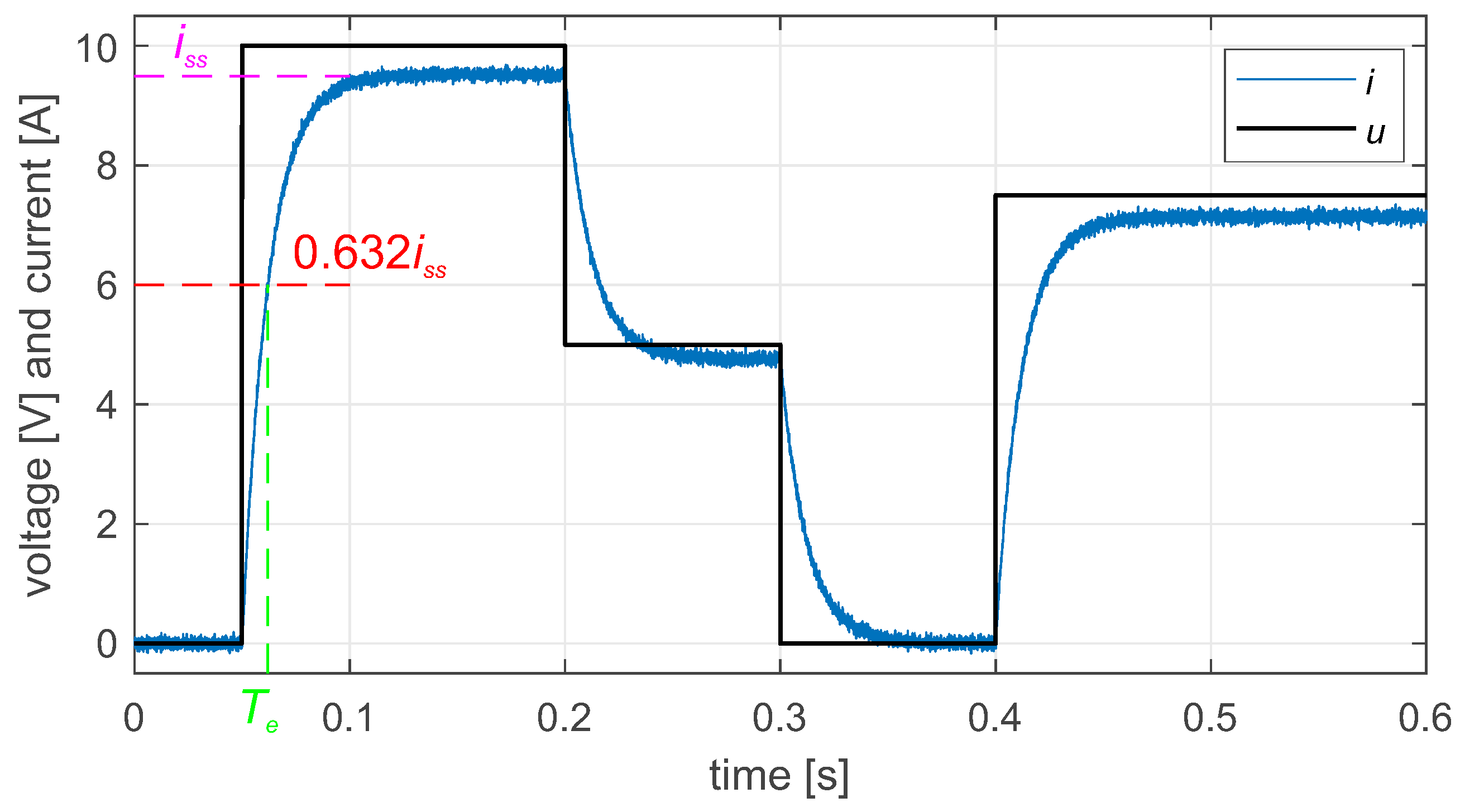
Figure 2.
Drive’s velocity step response.
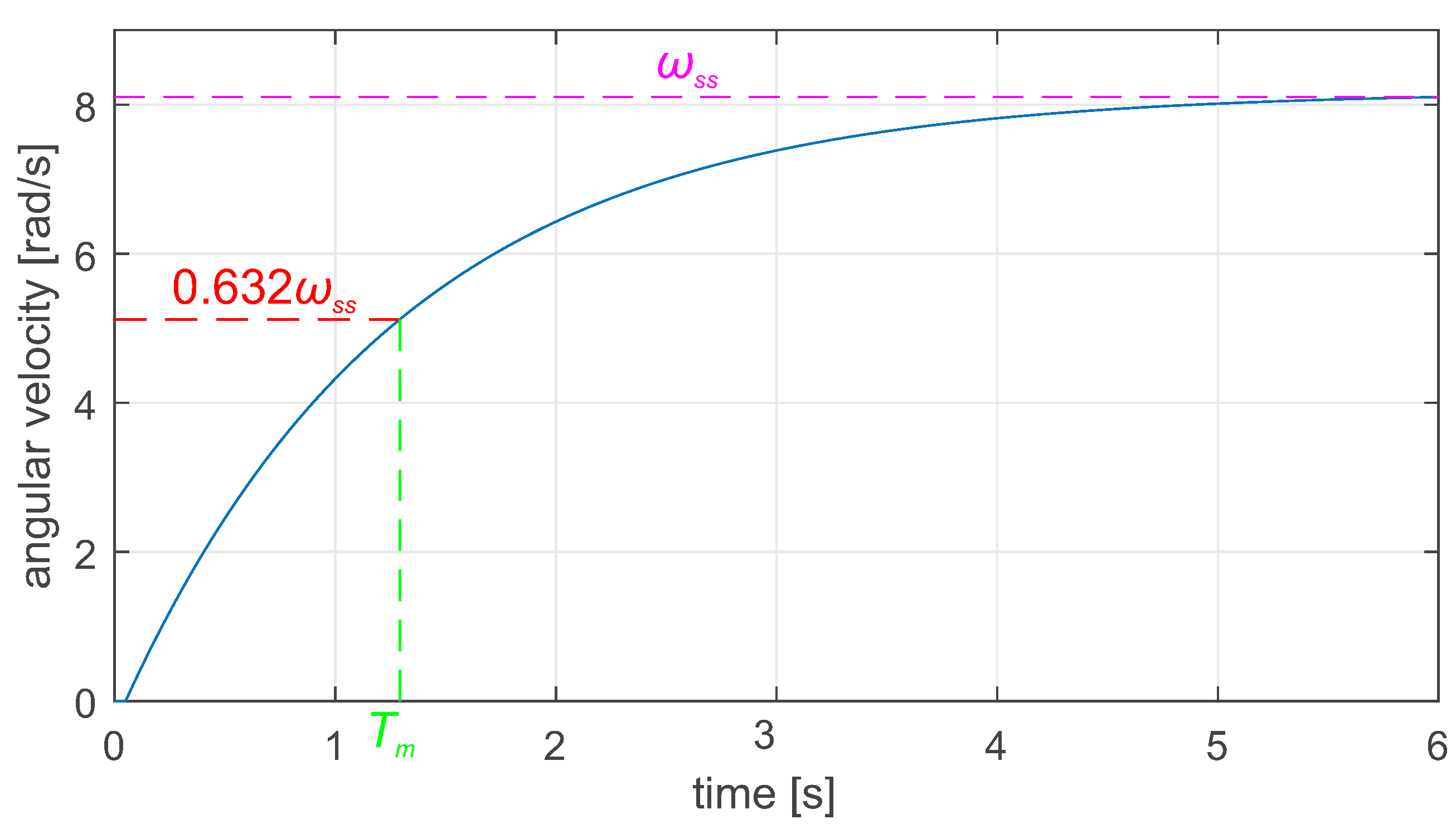
Figure 3.
Cascade control structure.
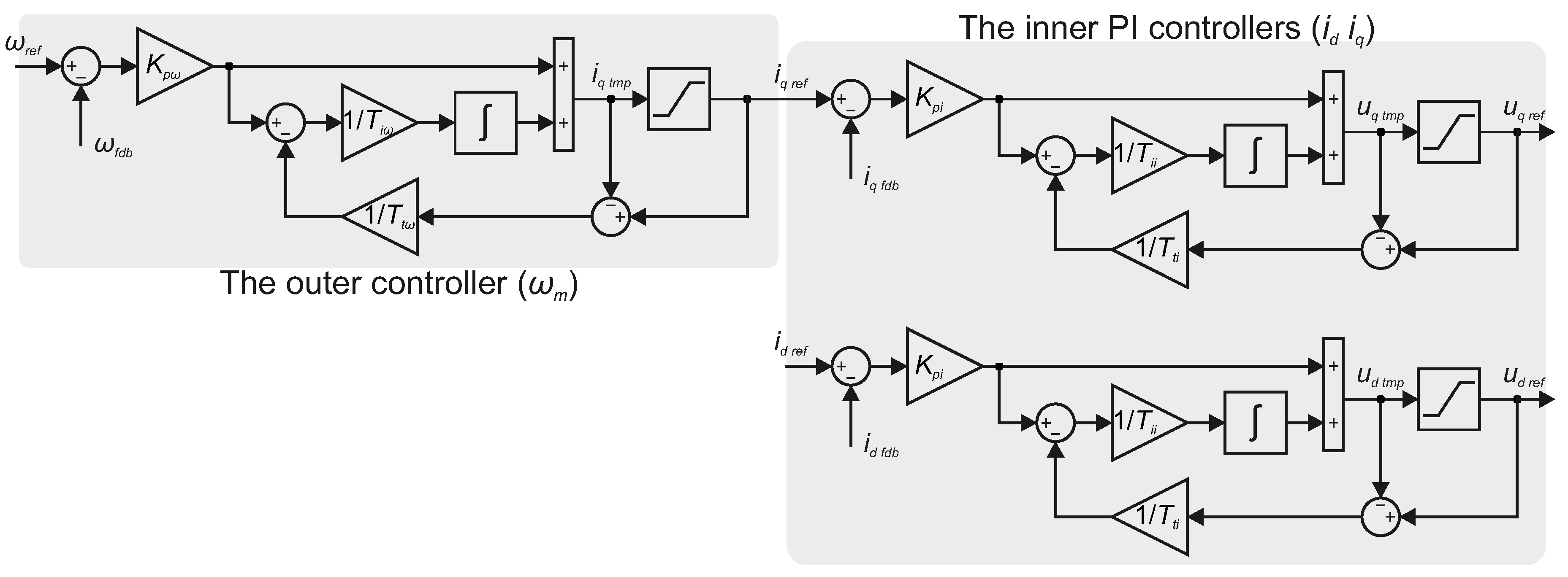
Figure 4.
SBMA’s general flowchart.
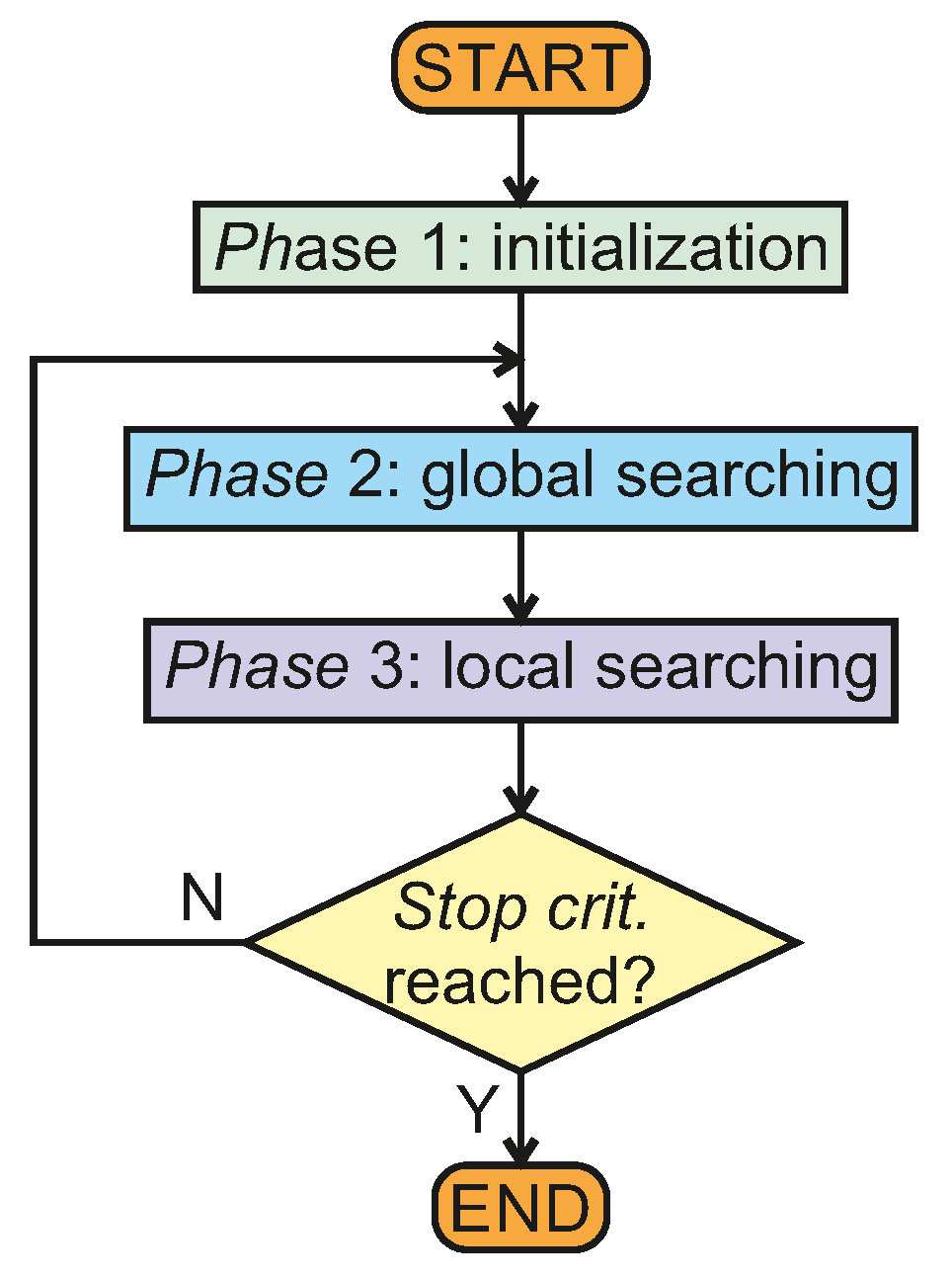
Figure 7.
LLM’s evaluation flowchart.
Figure 8.
Step responses of PMSM drive with cascade control structure tuned using LLM’s: (a), (c), and (e) angular velocity, (b), (d), and (f) space vector current components.
Figure 8.
Step responses of PMSM drive with cascade control structure tuned using LLM’s: (a), (c), and (e) angular velocity, (b), (d), and (f) space vector current components.
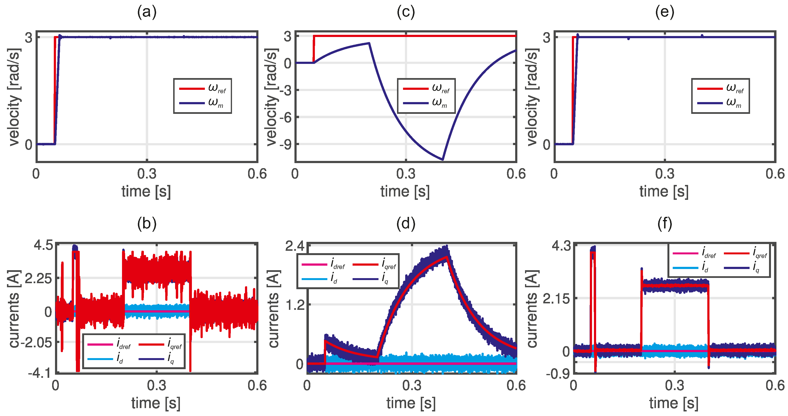
Table 1.
Parameters of the angular velocity and the currents PI controllers obtained by the users.
| No. | Auto-tuning* | Method | Iter. no. | Time [mins] | User exp. | Figure | |||||||
|---|---|---|---|---|---|---|---|---|---|---|---|---|---|
| 1 | 5.58 | 82.85 | 1 | 30.89 | 1000 | 1 | 0.00197 | N | Ordemio | – | adv | Figure 8 (e)-(f) | |
| 2 | 0.5 | 200 | 1 | 30 | 200 | 1 | 0.00198 | Y | empirical | 74 | 80 | beg | – |
| 3 | 0.9 | 45 | 0 | 350 | 4 | 0.8 | 0.00198 | Y | empirical | 80 | – | beg | – |
| 4 | 217.15 | 0 | 371.45 | 134.49 | 500 | 3.16 | 0.00198 | Y | ABC | 500 | 70 | adv | Figure 5 (e)-(f) |
| 5 | 0.39 | 144.44 | 0.1 | 210.1 | 0.0001 | 1 | 0.00199 | N | analytical | 80 | – | beg | – |
| 6 | 8.37 | 0.0001 | 1000 | 382.29 | 0.0004 | 100 | 0.002 | N | analytical | 109 | 30 | beg | Figure 6 (e)-(f) |
| 7 | 2.79 | 82.85 | 0.8 | 152.72 | 1098 | 0.5 | 0.002 | N | analytical | 32 | – | beg | – |
| 8 | 278.96 | 82.85 | 3.37 | 388.98 | 388.98 | 1 | 0.0021 | N | ChatGPT | – | adv | Figure 8 (a)-(b) | |
| 9 | 0.56 | 82.72 | 0.8 | 15.29 | 109.86 | 1.12 | 0.0021 | N | analytical | 41 | 50 | beg | – |
| 10 | 0.5 | 231.11 | 7 | 15.29 | 109.86 | 1.27 | 0.0021 | N | analytical | 70 | – | beg | – |
| 11 | 0.23 | 82.72 | 0 | 152.97 | 0.0009 | 20 | 0.0021 | N | analytical | 34 | 71 | beg | – |
| 12 | 0.28 | 120.7 | 1 | 16.97 | 549.31 | 50 | 0.0022 | N | analytical | 27 | – | beg | – |
| 13 | 2.8 | 82.7 | 0 | 5493.1 | 0.0002 | 5 | 0.0022 | N | analytical | 37 | 56 | beg | – |
| 14 | 2.5 | 12.5 | 0.7 | 17.5 | 25 | 1.25 | 0.0023 | N | empirical | 42 | 15 | adv | – |
| 15 | 0.5 | 60 | 62 | 10 | 120 | 190 | 0.0026 | Y | empirical | 120 | – | beg | – |
| 16 | 1 | 300 | 5 | 20 | 100 | 40 | 0.0026 | Y | empirical | 93 | – | adv | – |
| 17 | 0.4 | 185 | 30 | 150 | 90 | 30 | 0.003 | N | empirical | 115 | 75 | beg | – |
| 18 | 0.75 | 38.52 | 0 | 44.7 | 92.52 | 0 | 0.003 | N | analytical | 98 | – | beg | – |
| 19 | 0.47 | 963.65 | 19.56 | 5.81 | 94.45 | 19.96 | 0.003 | N | analytical | 14 | – | adv | Figure 6 (c)-(d) |
| 20 | 0.056 | 82.85 | 0.7 | 17.5 | 27.5 | 1.5 | 0.0032 | N | an. & em. | 55 | 10 | adv | – |
| 21 | 0.35 | 750 | 200 | 100 | 110 | 190 | 0.0034 | Y | empirical | 91 | 60 | beg | – |
| 22 | 1.21 | 44.95 | 1 | 7.73 | 45.14 | 15 | 0.0042 | Y | PSO | 2757 | 120 | adv | Figure 5 (c)-(d) |
| 23 | 0.103 | 82.72 | 0 | 5 | 50 | 1 | 0.0044 | N | an. & em. | – | 45 | adv | Figure 6 (a)-(b) |
| 24 | 1.4 | 82.72 | 0 | 15.29 | 1.4 | 5 | 0.0045 | Y | analytical | 47 | 66 | beg | – |
| 25 | 0.36 | 250 | 65 | 75 | 30 | 100 | 0.0091 | Y | empirical | 238 | 75 | beg | – |
| 26 | 0.019 | 11.88 | 40.42 | 9.47 | 37.86 | 189.86 | 0.013 | N | ABC* | 430 | 24 | adv | Figure 5 (a)-(b) |
| 27 | 0.011 | 82.72 | 0.1 | 3.05 | 0.046 | 0 | 0.054 | N | analytical | 13 | 48 | beg | – |
| 28 | 0.28 | 82.85 | 1 | 0.3 | 0.8 | 1 | 3.22 | N | an. & em. | 21 | 16 | adv | – |
| 29 | 0.64 | 3.81 | 3.81 | 0.16 | 0.12 | 0.12 | 10.72 | N | Copilot | – | adv | Figure 8 (c)-(d) |
* The coefficients obtained from ABC (row 26) were applied if auto-tuning is used.
Disclaimer/Publisher’s Note: The statements, opinions and data contained in all publications are solely those of the individual author(s) and contributor(s) and not of MDPI and/or the editor(s). MDPI and/or the editor(s) disclaim responsibility for any injury to people or property resulting from any ideas, methods, instructions or products referred to in the content. |
© 2024 by the authors. Licensee MDPI, Basel, Switzerland. This article is an open access article distributed under the terms and conditions of the Creative Commons Attribution (CC BY) license (http://creativecommons.org/licenses/by/4.0/).
Copyright: This open access article is published under a Creative Commons CC BY 4.0 license, which permit the free download, distribution, and reuse, provided that the author and preprint are cited in any reuse.


