
Submitted:
02 September 2025
Posted:
02 September 2025
You are already at the latest version
Abstract
The increasing adoption of high-performance DC motor control in embedded systems has driven the development of cost-effective solutions that extend beyond traditional software-based optimization techniques. This work presents a refined hardware-centric approach implementing real-time particle swarm optimization (PSO) directly executed on STM32 microcontroller for DC motor speed control, departing from conventional simulation-based parameter tuning methods. Novel hardware-optimized composition of an interval type-2 fuzzy logic controller (FLC) and a PID controller is developed, designed for resource-constrained embedded systems and accounting for processing delays, memory limitations, and real-time execution constraints typically overlooked in non-experimental studies. The hardware-in-the-loop implementation enables real-time parameter optimization while managing actual system uncertainties in controlling DC micro-motors. Comprehensive experimental validation against conventional PI, PID, and PIDF controllers, all optimized using the same embedded PSO methodology, reveals that the proposed FT2-PID controller achieves superior performance with 28.3% and 56.7% faster settling times compared to PIDF and PI controllers, respectively, with significantly lower overshoot at higher reference speeds. The proposed hardware-oriented methodology bridges the critical gap between theoretical controller design and practical embedded implementation, providing detailed analysis of hardware-software co-design trade-offs through experimental testing that uncovers constraints on low-cost microcontroller platform.
Keywords:
Experimental DC motor control
; hardware-software co-design
; STM32 microcontroller
; embedded Interval Type-2 FLC
; low-cost prototyping
1. Introduction
Rising demands in green energy generation, electric vehicles [1], transportation, construction, consumer electronics and industrial automation are bolstering the need for high performance, robust and high quality motors. Direct Current (DC) motors, even though they are one of the oldest electric motor designs, are still more than relevant in modern industry. Their market is experiencing steady growth, attributed to a broad range of application areas such as as robotics, military, spacecrafts [2], medical equipment, agriculture [3], unmanned monitoring systems [4]. The global push towards sustainable practices combined with the rising prevalence of electric vehicles are influencing the adoption of DC motors. Their main advantages in comparison with other types of motors are; small noise operation, low cost, better characteristics of speed and torque, good controllability, fast response in dynamic changes, high power-to-weight ratio, no requirement for current excitation and adequate performance for their cost.
Yet open loop method is being used for controlling brushed and brushless DC motors. Despite the simplicity of this approach, open loop systems lack of accuracy especially in dynamic or unpredictable applications. Another major disadvantage is the susceptibility to external factors. This vulnerability to variations and disturbances in load conditions leads to decreased system performance. The lack of feedback limits adaptability, since open loop systems are not adaptable to changing conditions. Meanwhile, wear and tear can not get compensated, hence manual tuning is required. Therefore, the aforementioned reasons in recent years have draw attention to closed loop control [5]. The presence of feedback loop provides enhanced precision, accuracy and adaptability to varying conditions. Disturbances can get compensated and stable performance is maintained, even in dynamic environments. Additionally, robustness is achieved, which is essential in robotics, automation, electric vehicles, medical equipment, computer numerical control machines. Sensorless DC motor controllers offer simplicity and cost-effectiveness [6,7]. These controllers rely on motor’s back electromotive force (EMF) or other internal characteristics to estimate the position of the rotor, i.e. without using external sensors. However, sensorless controllers do not perform well at low speeds. The motor appears “jumpy” or “jittery”, which is also known as “cogging”. Additionally, during rapid load changes, the lack of sensor results in less precise control. In sensored operation, motor operation is smooth, while stuttering and vibrations are significantly reduced. Sensor feedback enhances stability, leading to better response to load variations. Due to these reasons, over the last few years a greater focus has been placed on sensored closed loop controllers [8,9]. Reliable performance is ensured, while accurate and precise control may be achieved even at low speeds.
Traditionally, the most common control methods, used in the majority of studies, are the PI and PID controllers [10,11,12]. These conventional controllers are well known as common techniques for non-linear systems control, mainly due to their simple architecture and the easily managed control algorithm. However, PID controllers are sensitive to measurements errors and noise, causing crucial performance deterioration, instabilities and undesired oscillations [13]. Additionally, derivative filtering is proposed in [14,15,16], significantly enhancing robustness and improving stability. Parallel and coupling PID controllers were proposed in [17], while in [18] an approach using backstepping sliding mode control was demonstrated. Observer-based non linear controllers have also been employed in [19,20], providing immunity against measurement noise.
In recent years, much research has been performed on artificial intelligence (AI) control methods. Embedded artificial intelligence is impacting the future of every industry and every human being. Autonomous cars, robots, virtual nursing assistants, diagnosis of diseases, virtual tutors in education and customer services are some current and future applications. The main advantage of AI controllers is their robustness [21], being capable of overcoming the uncertainty of conventional control methods and providing better system response [22,23]. Commonly implemented methods use structures based on neural networks, fuzzy logic, genetic algorithms or even hybrid approaches. Fuzzy logic controllers (FLC) for DC motor control has been employed in [24,25], towards improved controller’s performance. The problem of disturbances has been addressed in [26]. FLC’s superiority over conventional PID controllers have been experimentally validated in [27]. Novel neural network controllers were examined in [28,29,30], while recently [22,31] genetic algorithm approaches were demonstrated. The robustness of neuro-adaptive controller was experimentally proved in [32]. In [33] a hybrid controller, consisting of a parallel combination of sliding mode and neurofuzzy controllers, was proposed.
Fuzzy logic controllers execute the control process by utilizing linguistic expressions along with the processes of fuzzification, rule base, and defuzzification [34]. These controllers provide an excellent way of dealing with imprecision and nonlinearity in complex control situations [35]. Despite the apparent advantages of Type-1 (IT1) FLC’s, it has been proved that they are not capable of fully handling the impact of uncertainties. [36,37]. In recent studies interval Type-2 (IT2) FLC’s outperformed IT1-FLC’s [38,39,40] mainly attributed to the crisp values of their membership grades of IT1-FLC’s. While the membership functions of Type-1 FLCs are certain, the membership functions of Type-2 FLCs are fuzzy themselves. Type-2 FLC’s have primary membership functions (PMF’s), which might be any value in the interval [0, 1]. Moreover, in PMF’s there is a secondary membership functions (SMF), defining the probability of PMF’s. The latter leads to an increased computational burden and as a result zero or unity SMF’s are developed. The combination of a conventional PID and a fuzzy system led to the creation of Fuzzy PID (FPID) [41,42,43]. Adaptive fuzzy controllers were presented in [44,45], providing robustness and improved control performance. In this paper, a composition of an interval Type-2 FLC and a PID controller is proposed to manage uncertainties in controlling the DC micro-motor under study. PID controller parameters are dynamically set by fuzzy sets, improving performance, robustness and systems response.
In recent literature numerous efforts in closed loop DC motor control development have been conducted, either by means of simulations [46,47,48], or in experimental configurations [49,50,51]. The former approaches, even though valuable to prove the conceptual design, use either low-cost development boards, which have hardware constraints and especially memory limitations, or expensive FPGA development boards which are considered as “overkill” for these type of applications. On the other hand, modern families of microcontrollers (e.g. like STM32 provided by STMicroelectronics), keep pace with emerging trends and remain at the forefront of embedded systems development, providing an ideal balance between cost, performance, scalability and dependability as presented in [52,53,54].
Although, a few control algorithms applied on experimental setup have been suggested, the amount of research analyzing practical difficulties and limitations either in hardware or software level, while proposing a clear methodology and design optimization techniques, is limited. Considering cases, in which readymade solutions are costly or insufficient due to custom application specifications, a low cost, fully flexible, customizable and parametrised prototype should be build. Based on the aforementioned factors, the key contributions of this paper are:
- Present refined hardware-in-the-loop approach, integrating real-time PSO directly on STM32 microcontroller, with comprehensive hardware-software co-design analysis highlighting constraints and trade-offs.
- Develop novel optimized hybrid FT2-PID controller tailored for embedded platforms.
- Validate the proposed FT2-PID controller against PI, PID, and PIDF controllers showing significantly faster settling times and reduced overshoot at higher reference speeds.r
- Address critical hardware limitations, including processing time, memory constraints, and real-time execution challenges, being overlooked in theoretical studies.
It should be highlighted that -to the authors’ knowledge extend- in research literature, similar efforts offering valuable technical competence are not found. In this paper, an adaptive IT2-PID controller is especially designed and experimentally implemented for coreless DC micro-motor (though the procedure can be easily applied to other DC motor types). Prioritizing cost and simplicity, hardware limitations and components selection are detaily presented. This proposed controller is being compared with PI, PID and PID with D filtering controllers, all being tuned using embedded real time PSO algorithm [55]. Discrete reference speed cases are being investigated not only to present the robustness of the controller under investigation but also to compare the microcontroller’s performance and resources needed. Emphasis is being given to microcontroller’s system-level characteristics and to hardware considerations for the prototype design. Parameters such as pulse width modulation (PWM) bit resolution, interrupt time selection for speed measurements, encoder’s resolution, experimental speed data filtering are also examined and pointed out. Finally, the design and the level of goodness of a microcontroller embedded adaptive IT2-PID is discussed.
The structure of this paper is as follows. A brief theory of DC micro-motor is presented in Section II, while the control strategies are discussed in Section III. Prototype design and development is described in Section IV. Section V presents the software development considering hardware limitations. The derived results are reported and commented in Section VI and ultimately Section VII serves to conclude the work.
2. Brief DC Micro-Motor Theory Overview
DC micro-motors represent a class of miniature motors that offer significant advantages over conventional DC motors, particularly in applications requiring compact size, high efficiency, and precise control. These motors are typically characterized by their small dimensions, with diameters ranging from a few millimeters to several centimeters, making them ideal for use in miniature devices and systems. They are known for their lightweight construction, which is often achieved by using specialized materials such as precious metals for the commutator and brush assembly, including platinum, silver, and gold. This contributes to reduced wear and tear, increased durability, and improved performance in high-speed applications. The design of these motors often incorporates permanent magnets in the stator, and their compact rotor design reduces energy losses while enhancing torque production. The small size of DC micro-motors allows for precise control over speed and positioning, making them particularly suitable for applications in robotics, medical devices, and embedded systems where space and efficiency are critical. Figure 1 presents the equivalent circuit and the investigated micro-motor.
The DC micro-motor under study, along with its equivalent circuit, is shown in Figure 1. The armature winding is characterized by its winding resistance () and inductance (), where the supply voltage () is introduced. The back electromotive force () induced in the armature winding arises from the interplay of the armature’s motion with the magnetic field. As the armature rotates within the magnetic field, it cuts through magnetic flux lines, which induces a voltage that opposes the applied voltage. This back electromotive force maintains a direct proportionality to the magnetic flux () and to the angular velocity (), which can be expressed as the rate of change in shaft position ().
The rotational speed (), expressed in revolutions per minute (rpm), is related to the angular velocity () using the equation below:
The back-emf coefficient () is a constant that represents the proportionality between the motor’s rotational speed and the induced electromotive force, reflecting the motor’s design and the strength of its magnetic field. This constant defines the relationship between the motor’s angular velocity () and the back electromotive force () generated. The back-emf is directly proportional to the motor’s rotational speed and the relationship is described by the following equation:
The armature current () is determined by the applied supply voltage (), the armature winding resistance (), its inductance (), and the back-emf () generated. The total applied supply voltage must counteract the resistive losses in the armature winding (), the inductive voltage drop caused by the time rate of change of the armature current (), and the back-emf. This relationship can be expressed as follows:
The back-emf reflects the conversion of electrical energy into mechanical energy, with its magnitude being directly influenced by the motor’s speed. The magnetic flux () is related to the coefficient , which governs the conversion between the armature current and the electromagnetic torque () generated by the motor. The mechanical dynamics of the motor are described by the following set of equations, where is the viscous damping coefficient, denotes the moment of inertia of the rotor, and represents the load torque:
By combining the electrical and mechanical equations, the following differential equations are obtained, which fully describe the system dynamics:
Upon applying the Laplace transform to Equations (7) and (8), the transfer function of the motor is derived, which relates the motor speed to the applied input voltage:
The transfer function is commonly depicted in block diagram form, as illustrated in Figure 2. In this diagram, the supply voltage () serves as the input, while the micro-motor’s rotational speed () serves as the output. Accurate modeling of the motor necessitates identifying six parameters: , , , , , and . The specific parameter values for the DC micro-motor utilized in this work are provided in Table A1.
3. Control Strategies
3.1. Closed-Loop Control for Micromotor Speed Regulation
The objective of the controller under study is to regulate the DC micro-motor speed to a specified reference value by employing a closed-loop negative feedback control system. In the context of this study, the controller employs two inputs to determine the control action: the error and the change in error. The error is expressed as the difference between the measured rotational speed () and the reference rotational speed ().
Respectively, the change in error, which describes how the error changes over time, is calculated as:
The controller processes the error signal to generate the control signal . To interface with the DC micro-motor, a converter is incorporated between the controller and the motor, translating the control signal into the appropriate input voltage . This converter reconciles the voltage and current mismatches, ensuring the control signals are properly scaled to to meet the power requirements and drive the micro-motor. The negative feedback structure dynamically adjusts the control action based on the deviation between the reference and measured micro-motor speed, thereby minimizing the error signal . This closed-loop mechanism compensates for external disturbances, system nonlinearities, and load variations, ensuring accurate and stable speed regulation. Additionally, the feedback system enhances the motor’s response to dynamic changes in speed, enhancing steady-state accuracy and robustness against fluctuations.
Figure 3 presents the schematic of the negative feedback control loop used. The diagram illustrates the interconnections between key system components, including the controller, converter, DC micro-motor, and speed sensor. This closed-loop configuration ensures motor speed control by continuously comparing the reference speed with the measured speed.
3.2. PI, PID, and PIDF Controllers
In industrial applications, proportional integral controllers (PI) are among the most widely adopted control strategies due to their simplicity and effectiveness in reducing steady-state error. The PI controller works by combining two fundamental control actions: proportional control and integral control. The proportional term addresses the current error in the system by generating an output directly proportional to the current error. The error signal is multiplied by a constant, , known as the proportional gain. This relationship is given by:
The term represents the Laplace transform of the error signal . While the proportional term effectively reduces error in the short term, it does not address persistent, steady-state errors that may arise. To tackle this issue, the integral term is introduced. The integral action accumulates the error over time and provides corrective action to eliminate any steady-state offset. This action is represented as:
When combined, the overall output of the PI controller, , is given by:
This combination of proportional and integral terms delivers balance between quick responsiveness and sustained accuracy. The PI controller is particularly effective in systems where the error changes slowly or remains constant over time. However, the PI controller faces limitations in systems where the error changes rapidly. Since it lacks a term that responds to the rate of change of the error, the controller may exhibit slower response times, higher overshoot, and longer settling times in dynamic systems. To enhance the performance of the PI controller in more dynamic systems, the proportional-integral-derivative (PID) controller is introduced. The PID controller builds on the PI controller by incorporating a derivative term that responds to the rate of change of the error. This term helps the controller anticipate future error trends, allowing it to adjust more quickly and precisely to changes in the system. The derivative term contributes to system stability by limiting overshoot and advancing transient response. It is mathematically expressed as:
Thus, the output of the PID controller becomes:
Conventional PID controllers frequently struggle to handle the intricate dynamics of DC motors, leading suboptimal performance [56]. While the derivative term improves the system’s responsiveness and stability, it can also amplify high-frequency noise, resulting in oscillations or unwanted vibrations in the control signal. To address these challenges, a derivative filter can be introduced. This filter smooths the high-frequency components of the derivative term, reducing the controller’s sensitivity to noise and mitigating undesirable oscillations. The resulting controller, known as the Proportional-Integral-Derivative-Filter controller (PIDF), is mathematically expressed as:
Here, N represents the filter coefficient, which determines how much high-frequency noise is filtered out from the derivative term in the PIDF controller. The filter is typically employed to avoid undesirable oscillations or instability caused by noise amplification in the derivative term. The value of N creates a trade-off between noise suppression and the controller’s responsiveness. Table 1 summarizes the advantages and disadvantages of selecting small or large values of N.
The PIDF controller is particularly effective in DC motor control applications where precise speed regulation is required despite fluctuations in load or noise in the feedback signal. By incorporating a derivative filter, it suppresses high-frequency noise that can otherwise destabilize the control loop. This controller strikes a balance between rapid error correction and maintaining stability, enabling the controller to achieve accurate motor operation while adapting to changes in reference speed or system disturbances. Figure 4 shows the structure of the examined controllers.
3.3. FT2-PID Controller
Fuzzy logic is a computational model based on approximate reasoning rather than fixed, exact rules. It manages uncertainty and imprecision, making it effective in complex control systems. Unlike traditional controllers that require precise mathematical models, fuzzy logic handles ambiguity, imprecise measurements, and noisy data. Using linguistic variables and fuzzy rules, it adapts well to systems with nonlinearities and disturbances, where conventional methods like PID may falter.
In essence, fuzzy logic control operates through three key stages: fuzzification, inference, and defuzzification. During fuzzification, precise input values are transformed into fuzzy representations using membership functions (MFs) that describe the degree of membership within a given range, typically [0, 1]. Complete membership in a fuzzy set is denoted by 1, while 0 reflects no membership. In the inference stage, a rule base consisting of conditional relationships is applied to the fuzzified inputs. These relationships define how the inputs correspond to the outputs, with the inference engine processing them to generate the corresponding fuzzy outputs. In this work, the process follows the Mamdani fuzzy inference system, which combines these rules to derive fuzzy control actions. Finally, in the defuzzification phase, the fuzzy outputs are translated into a precise, crisp value, which serves as the final control signal, enabling accurate system control.
Interval Type-2 Fuzzy Logic (IT2-FL) extends traditional fuzzy logic by introducing an additional dimension of uncertainty within its membership functions. While Type-1 fuzzy logic employs precise membership grades to map input values to fuzzy sets, IT2-FL utilizes interval-valued membership functions to account for uncertainties inherent in real-world data. This framework captures both the primary membership values and their associated uncertainties, thereby enabling a more nuanced representation of vagueness and imprecision.
Uncertainty in these sets is characterized using key parameters. The mean () represents the central value of the membership function, serving as the core membership value around which the fuzzy set’s membership degrees vary. The standard deviation () quantifies the spread of membership values around the mean, with larger indicating greater uncertainty. The delta () represents the uncertainty interval, describing the deviation in the mean membership value. Figure 5 shows IT2 gaussian membership functions, with the left image representing uncertainty in the mean and the right image depicting uncertainty in the standard deviation.
In this work uncertainty in the mean is used, with the centers of each membership function expressed as:
where and represent the centers of each MF, is the mean, and is the uncertainty in the mean. The standard deviation is assumed to remain the same across both membership functions. The membership function of an interval type-2 fuzzy set defined over the input domain F and output domain G can be expressed as:
where and are secondary membership intervals that account for the uncertainty in the primary memberships and , respectively. These fuzzy sets are defined over the domains F and G, which represent the input and output spaces, respectively. The relationship between inputs and outputs is governed by a set of fuzzy rules, commonly represented as . A typical rule is formulated as:
where are interval type-2 fuzzy sets associated with the inputs, and represents the output fuzzy set. These rules form a rule base that enables the inference process, ultimately producing a fuzzy output that is defuzzified into a crisp control signal.
The IT2-FLC structure is illustrated in Figure 6. The diagram demonstrates the process by which crisp inputs are transformed into fuzzy values, processed through the inference system, and subsequently converted back into crisp outputs. The arrows illustrate the transfer of information across these stages. In this study, an Interval Type-2 Fuzzy Logic-based PID (IT2-PID) controller is implemented, integrating the adaptive capabilities of Interval Type-2 Fuzzy Logic (IT2-FL) with the proven effectiveness of the PID control framework. The IT2-PID controller dynamically adjusts the proportional (), integral (), and derivative () gains through a Type-2 fuzzy inference system. This enables real-time adaptation of the control parameters to varying system conditions, ensuring robust and precise control. The proposed structure of the IT2-PID controller is depicted in Figure 7.
The proposed IT2-FLC accepts two inputs: the error (e) and the change in error (). The output of the controller is a scalar value referred as the PID Tuning Index (). The standard deviation () is set to 250 for the error and 25 for the change in error MFs, while the delta () values are 62.5 and 6.25, respectively. MFs and the inference system surface are depicted in Figure 8. The rule base governing the IT2-FLC is presented in Table 2.
Since lies within the range , parameter mapping is required to determine the appropriate PID gains (, , and ). The absolute value of the PID Tuning Index () is utilized. This ensures that the tuning decisions depend only on the magnitude of the index, independent of its sign. The absolute value is divided into predefined intervals, with each interval corresponding to a unique set of PID parameters. The selection of parameter sets is performed dynamically based on the magnitude of . Table 3 presents the mapping framework between the intervals of and the corresponding PID parameter sets. Tuned parameter values will be presented in Section VI. The resulting parameters are stored and dynamically selected at runtime.
4. Prototype Design and Development
The hardware system’s topology, as shown in Figure 9, illustrates the interconnected components necessary for the control and operation of the DC micro-motor. At the heart of the system, a microcontroller functions as the central processing unit, responsible for acquiring, processing, and transmitting various signals. The microcontroller interfaces with a rotary encoder, which monitors the micro-motor’s speed and delivers real-time feedback. Given the micro-motor’s higher voltage and current demands compared to the microcontroller, a dedicated power supply and a robust motor driver circuit are included to ensure proper operation of the motor. The system’s capability to monitor motor performance is enhanced by an oscilloscope, which facilitates the acquisition of speed and current data. Since the oscilloscope operates in the analog domain, a digital-to-analog converter (DAC) is employed to bridge the gap between the digital signals generated by the microcontroller and the analog signals required by the oscilloscope.
Furthermore, the system incorporates multiple power supplies to meet the diverse power requirements of the various components. A dedicated power supply is allocated for the DC micro-motor, while two buck converters provide 5 V and 12 V to power the peripheral devices, ensuring stable and efficient operation of the entire system. The following sections will delve into the specifics of each hardware module, offering a comprehensive analysis of their design considerations, operational principles, and role within the overall system architecture. Figure 10 shows the experimental testbench setup.
4.1. Microcontroller
The selection of the microcontroller was based on several critical criteria: a) external hardware interrupts for speed measurement, as the encoder generates square pulses, b) software interrupts, required not only for speed measurement but also for the controller’s time-discrete actions, c) sufficient number of general-purpose digital input/output pins, including at least one output pin with PWM capability, d) fast processing and enough memory to meet the application requirements, e) low cost and market availability. Considering these factors, the STM32F103C8 from STMicroelectronics was selected. The detailed microcontroller specifications are presented in Table 4.
4.2. Power Supply
The NPS306W digital DC power supply is selected for its capacity to provide stable and sufficient power for the coreless DC micro-motor, with a maximum output of 30 V and 6 A. In addition, two buck-boost voltage regulation modules supply the necessary 5 V and 12 V for peripheral components. These regulated power levels are essential for powering the DAC, current sensor, motor driver, and rotary encoder, which together support the motor’s control and monitoring.
4.3. Driver, Sensors, and Peripherals
DC motors demand high voltage and current, whereas microcontrollers operate on low-power signals. To address this mismatch, the BTS7960 H-bridge motor driver is used to convert the low-power signals from the microcontroller into high-power signals capable of driving the motor.This driver efficiently converts the low-power control signals from the microcontroller into high-power signals capable of driving the motor. The BTS7960 is well-suited for the application, as it supports bidirectional motor control, operates within the required voltage and current range, and can handle a PWM frequency of up to 25 kHz, all while maintaining cost-effectiveness and wide availability. For precise monitoring of the motor’s speed, the OMRON E6A2-CW5C rotary encoder is integrated into the system, providing 200 pulses per rotation to accurately measure the rotational speed. Data acquisition is a critical aspect of system performance evaluation, and for this purpose, the RIGOL DS1054Z oscilloscope is selected. With four channels, a 50 MHz bandwidth, and a sampling rate of 1 GS/s, the oscilloscope is used to capture and display both the microcontroller’s control signals and the motor’s real-time speed and current characteristics. In addition, the ACS712 Hall-effect current sensor is chosen to measure the motor’s current, providing data for visual representation on the oscilloscope. This sensor measures currents up to 5 A with a sensitivity of 185 mV per ampere. Since the microcontroller generates only digital signals, a 10-bit MCP4725 digital-to-analog converter (DAC) is employed to convert the digital data into analog signals for oscilloscope visualization. The hardware components used are summarized in Table 5.
5. Software Development Considering Hardware Limitations
5.1. Software Development Philosophy
The control strategy for the micro-motor system is implemented through a modular software architecture, comprising four main routines: (a) the control loop routine, which includes PI, PID, PIDF, and FT2-PID control strategies, (b) the PSO tuning routine, (c) the Encoder Pulse Interrupt Service Routine (ISR), triggered by the rising edges of the encoder’s square pulses, and (d) the Time Interval ISR, executed at predefined intervals to filter and perform calculations on speed measurement data. Two initialization routines were developed for variable setup and interrupt configuration. The PSO routine is divided into two main subroutines: parameter initialization and objective calculation. The software was implemented in C using STM32CubeIDE, leveraging the STM32F103C8 microcontroller’s features. In particular, the platform’s customizable Pulse Width Modulation (PWM) generation capabilities streamlined the development of the examined DC micro-motor control algorithms. The software implementation is schematically represented in the flowchart in Figure 11.
5.2. Main Flowchart
The main program routine begins with the initialization of timers and variables, followed by setting the micro-motor’s reference speed. When tuning mode is enabled, the program executes the PSO tuning routine; otherwise, it proceeds directly to the setpoint of reference speed. Upon a new speed measurement is available, the program initiates the closed loop control routine. The workflow of the main routine is depicted in Figure 11a.
5.3. PSO Tuning Routine
Particle Swarm Optimization (PSO) is an algorithm inspired by the social dynamics observed in natural phenomena, particularly bird flocking and fish schooling. In this approach, each particle represents a potential solution to the optimization problem. The movement of a particle is influenced by two primary factors: its personal best position, which is the best solution it has achieved individually, and the global best position, representing the best solution identified by the swarm as a whole. By integrating individual experiences with the collective knowledge of the swarm, particles explore the solution space to achieve optimization. The goal of this process is to minimize the objective function, which in this study is the system’s settling time. The position and velocity of each particle are progressively modified through iterative updates, following the equations outlined below:
where:
- denotes the position of the i-th particle at time t,
- represents the velocity of the i-th particle at time t,
- w is the inertia weight, which adjusts the influence of the particle’s prior velocity,
- and are the cognitive and social coefficients, which determine the weight given to the personal best and global best positions in influencing the particle’s movement, respectively
- and have random values, uniformly distributed between 0 and 1, adding stochastic behavior to the algorithm,
- refers to the best position found by the i-th particle during its search,
- represents the best position found by the entire swarm.
The PSO tuning routine is illustrated in Figure 11b. First the Parameter Initialization Subroutine initializes the velocities and positions of the particles within the swarm. This process, presented in Figure 12a, includes randomizing the positions and velocities, and defining the bounds for the parameters being optimized. Additionally, this subroutine initializes the objective function and sets the initial positions for the personal best and global best solutions within the swarm. Then, the tuning reference speed setpoint is defined as 2750 rpm for this work. The system checks whether new speed measurements are available. If new measurements are available, the system checks whether the PSO iteration time has elapsed. Once the iteration time has passed, the Objective Calculation subroutine is triggered. This subroutine, depicted in Figure 12b, determines the fitness of each particle by measuring the settling time of the system. This settling time is then used as the fitness value, which guides the update of both the personal best position of the particle and the swarm global best position. The iterative process allows the particles to modify their positions according to their own experiences as well as the swarm’s collective knowledge. After each iteration, the system checks if the PSO iterations have been completed. If the iterations are not completed. Once the PSO iterations are completed, the tuned parameters are updated, and the routine ends. Table 6 summarizes the parameter values used in the PSO routine:
5.4. Closed Loop Routine
The closed loop routine, illustrated in Figure 13, is integral to the precise control of the micro-motor within this system. The process begins with the continuous reading of the motor’s speed, which provides real-time feedback to the system. Upon receiving the latest speed measurement, the routine retrieves the latest tuned controller parameters, ensuring that the controller operates with the optimal settings. Following this, the controller performs the necessary calculations based on the error between the reference and measured speeds. The computed control signal is then subjected to saturation limits to prevent excessive control actions that could destabilize the system. Finally, a PWM control signal is generated from the control signal. This signal is sent to the motor driver to adjust the motor’s voltage, thereby achieving the desired speed. This iterative process ensures accurate and responsive speed control, balancing performance and stability throughout operation.
STM32F103C8 offers fully customizable PWM pulse generation. PWM is utilized to control the micro-motor’s voltage with a specific degree of accuracy, facilitating the adjustment of micro-motor speed. The characteristics of the PWM signal, specifically its resolution and frequency, are determined by the microcontroller’s clock speed and the chosen resolution. The relationship governing this dependency is expressed in Equation 23:
Here, is the frequency of the PWM signal, represents the clock frequency of the microcontroller, and n denotes the bit resolution of the PWM. The bit resolution defines the granularity of the voltage control, while the PWM frequency is related to how smoothly the motor operates. Table 7 presents the achievable PWM frequencies for various bit resolutions, assuming a clock speed of 72 MHz.
The motor driver used in this system is capable of operating at frequencies as high as 25 kHz. To ensure compatibility while maintaining adequate resolution, a 12-bit resolution and a PWM frequency of 17.578 kHz are chosen. The resolution of the voltage control step is calculated using Equation 24, where is the nominal voltage of the micromotor, and corresponds to the resolution scale:
For an 18 V micromotor operating with 12-bit resolution, the voltage step is determined as follows:
This voltage step value influences the motor’s speed control precision. The relationship between the control speed step and the voltage step is described in Equation 26, where is the nominal speed of the motor:
By substituting the nominal speed of 5000 rpm and the voltage step of 4.39 mV, the control speed step is calculated as:
This calculated speed step of 1.22 rpm ensures that the system can provide sufficiently fine control over the micro-motor’s operation. The selected values balance the requirements for precision and system compatibility with the motor driver hardware.
5.5. Interrupt Services Routines
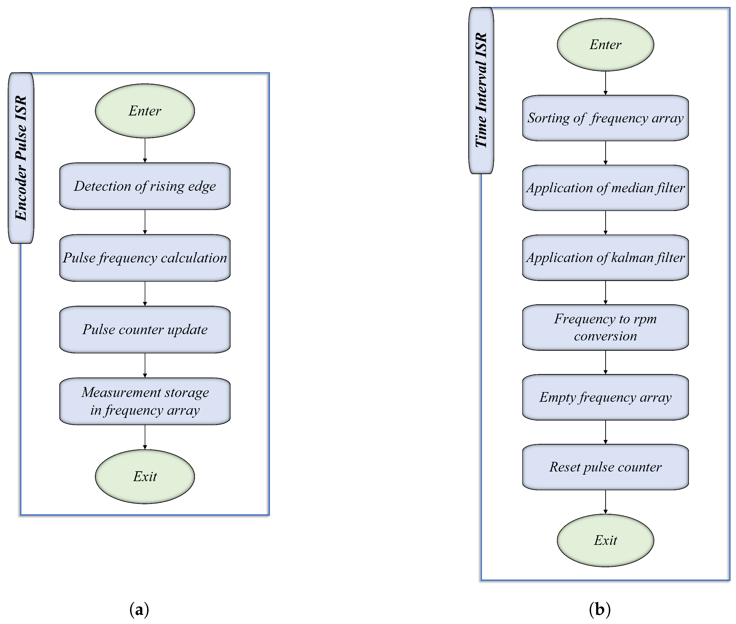
This category of routines manages two program interrupts, namely the Encoder Pulse ISR and the Time Interval ISR, which are both employed for measuring the speed of the DC micro-motor.
Figure 14.
Flowchart of the software routines for (a) Encoder Pulse ISR and (b) Time Interval ISR.
5.5.1. Speed Measurement Methodology
Figure 15 illustrates the proposed speed measurement principle. The rotary encoder produces square pulses which are directly proportional to the angular displacement of the micro-motor shaft. These pulses form the foundation for determining the micro-motor’s speed over a defined time interval, denoted as . During this interval, interrupts are triggered by the rising edges of the encoder’s pulse signal. Each interrupt represents a discrete event that is processed by the microcontroller, which measures the elapsed time between consecutive rising edges. The microcontroller records the amount of clock cycles () occurring between two rising edges. This count is used to calculate the frequency of encoder pulses () for a given speed as:
where is the clock frequency of the microcontroller. Given the encoder’s resolution () representing the number of pulses per full micro-motor revolution, the rotational speed () is calculated as:
5.5.2. Time Interval
During the time interval , the microcontroller calculates and stores multiple speed measurements. At the end of the interval, the collected data is processed, and a new speed measurement is obtained. Increasing the duration of this interval allows for the capture of a greater number of pulses, which enhances the accuracy of the calculated rotational speed. However, this improvement in measurement precision comes at the expense of control responsiveness, as the controller updates its actions only after each new speed measurement is available. Conversely, a shorter time interval provides more frequent speed updates, enabling the controller to respond more rapidly to changes in the system. However, this may reduce the accuracy of the speed measurements due to fewer captured pulses. Thus, the selection of represents a critical balance between measurement accuracy and control responsiveness, requiring careful optimization based on the application’s requirements. Table 8 summarizes the benefits and drawbacks of selecting small or large time interval values. Figure 16 illustrates the correlation between the selected time interval and the number of encoder pulses, based on the equation:
where is the number of encoder pulses generated within the time interval period. For this work, a of 2 ms is chosen, as it strikes a balance between measurement accuracy and control responsiveness.
5.5.3. Proposed Two-Stage Filtering Method
Raw data obtained from the rotary encoder often exhibit noise, particularly under dynamic conditions. To address this, a two-stage filtering method is proposed, combining a median filter with a Kalman filter. In the initial stage, raw data speed measurements are processed through the median filter () to eliminate outliers and suppress sporadic noise. Following the initial median filtering stage, the signal undergoes further processing using a Kalman filter. This stage enhances the reliability of the speed estimation by reducing the effect of high-frequency noise. The Kalman filter estimates the speed () using the following recursive equations:
where:
- K: Kalman gain, determining the weight of the new measurement,
- P: Estimate error covariance,
- Q: Process noise covariance,
- R: Measurement noise covariance.
- : Estimated speed at the current time step k,
- : Measured speed after the median filter at time step k.
The parameters listed in Table 9 were selected to optimize the performance of the Kalman filter in suppressing noise while preserving the responsiveness of the speed estimation process. These parameters strike a balance between sensitivity to dynamic changes and the stability of the estimated output. To evaluate the effectiveness of the proposed filtering approach, a step voltage was applied to the micro-motor, enabling a direct comparison between raw sensor data, single-stage Kalman filtering, and the proposed two-stage filtering method. As illustrated in Figure 17, the proposed method eliminates undesired spikes and significantly attenuates noise, resulting in a more stable and accurate speed estimation. The applied step voltage profile is shown in Figure 17b for reference.
6. Results and Discussion
6.1. PSO Real-Time Tuning
The Particle Swarm Optimization (PSO) algorithm was employed for real-time tuning of all evaluated controllers. This approach leverages the computational capabilities of the microcontroller to dynamically optimize controller parameters, with settling time serving as the optimization objective. The target speed for all controllers was set at 2750 rpm to ensure uniformity in performance assessment across different control strategies. The convergence times for PSO tuning of the four controllers are illustrated in Figure 18.
The results indicate that the PI and PID controllers achieve convergence within 30 seconds, highlighting their computational efficiency and simplicity. In contrast, the PIDF and FT2-PID controllers exhibit significantly longer convergence times, requiring approximately 7 minutes and 5 minutes, respectively. This disparity is attributed to the increased complexity of these controllers and the higher number of variables involved in their parameter optimization processes. The PSO tuning results for the PI, PID, and PIDF controllers are summarized in Table 10. For the FT2-PID controller, the Interval Type-2 Fuzzy Logic Control (IT2-FLC) framework described in Section V was employed to dynamically adapt the controller parameters (, , and ) based on the PID Tuning Index (). The index values, lying within , were mapped to parameter sets according to the intervals defined in Table 3. The PSO optimization focused on refining the fuzzy system to ensure optimal tuning intervals. Table 11 presents the tuned parameter values corresponding to each interval of .
6.2. Memory Usage and Analysis
The memory usage of the microcontroller was evaluated after uploading the control algorithms for all controllers, as well as during the Particle Swarm Optimization (PSO) real-time tuning. The results, presented in Table 12 and Table 13, highlight SRAM and Flash memory usage for the different controllers.
Table 12 presents the memory requirements for all controllers. The FT2-PID controller exhibits the highest memory consumption, requiring 3.20 KB of SRAM and 32.39 KB of Flash memory. This increased memory demand is primarily due to the higher computational complexity associated with fuzzy type-2 logic and additional tuning parameters. Table 13 shows the memory usage during PSO real-time tuning. SRAM usage increases by more than 58% for all controllers compared to standard operation. The FT2-PID controller, again, demands the most memory, with 7.86 KB of SRAM and 41.69 KB of Flash memory. These results suggest that the microcontroller’s memory is sufficient for all tested controllers in both standard operation and PSO real-time tuning. However, the significant rise in memory consumption during PSO tuning highlights the need for efficient resource management when deploying optimization techniques on embedded systems.
SRAM usage directly affects real-time performance due to its role in storing temporary variables, stack operations, and intermediate computations during controller execution. Flash memory, although less critical to runtime, shows notable consumption by the FT2-PID controller. During real-time tuning, it uses approximately 65% of the available Flash memory, while SRAM consumption for the FT2-PID controller reaches around 39% of the available memory.
Figure 19 provides a visual comparison of SRAM and Flash memory usage across all controllers. The FT2-PID controller consistently demonstrates the highest memory consumption in both SRAM and Flash categories. These findings highlight the trade-offs between advanced control performance and resource utilization, which must be carefully considered during system design. While all tested controllers are suitable for implementation on the selected microcontroller, the FT2-PID controller is the most resource-intensive. Future work could explore memory optimization techniques for fuzzy type-2 controllers, aiming to reduce memory usage while maintaining system performance and efficiency.
6.3. CPU Load Analysis
The CPU load was evaluated for all controllers to assess the computational demand imposed by each control algorithm. The outcomes are summarized in Table 14, which details the CPU load percentage at various motor speeds. Two configurations were analyzed: PI, PID, and PIDF controllers, and the FT2-PID controller. The data reveal that the CPU load increases with motor speed for all controllers. The FT2-PID controller exhibits a significantly higher CPU load compared to the PI, PID, and PIDF configurations. At a motor speed of 5000 rpm, the FT2-PID controller requires approximately 69.14% of the CPU resources, whereas the PI, PID, and PIDF controllers demand only 11.73%. This substantial difference of approximately 57.41% can be attributed to the added complexity of the fuzzy type-2 control logic and the associated computations required for its real-time operation.
At 1500 rpm, the CPU load for the FT2-PID controller is 57.72%, while the PI, PID, and PIDF controllers demand only 3.70%. This represents an increase of 54.02% in CPU load for the FT2-PID controller, further emphasizing the computational overhead associated with the fuzzy type-2 control algorithm. Similarly, at 3000 rpm, the FT2-PID controller consumes 61.11% of CPU resources, which is approximately 54.32% more than the 6.79% required by the other controllers. Figure 20 visually represents the CPU load variation with motor speed for all controllers. The FT2-PID controller’s computational overhead becomes evident as the motor speed increases, showcasing a steeper curve compared to the PI, PID, and PIDF controllers. The figure emphasizes the trade-offs between control complexity and computational efficiency, particularly for high-speed operations where the CPU is under significant load.
The increasing CPU load with motor speed highlights the importance of selecting computationally efficient algorithms, especially for high-speed applications. The PI, PID, and PIDF controllers demonstrate significantly lower CPU load across all tested speeds, making them more suitable for resource-constrained environments. However, the FT2-PID controller, despite its higher computational demand, offers the potential for superior control performance, particularly in systems requiring robust handling of uncertainties. These results underscore the trade-offs between computational resource utilization and control algorithm complexity. While the FT2-PID controller provides advanced features such as enhanced robustness and adaptability, its implementation on resource-limited microcontrollers necessitates careful consideration of CPU usage. This is particularly critical in applications where multiple tasks must run concurrently, as the high CPU load could limit the availability of processing power for other real-time operations.
In future work, optimization of the FT2-PID algorithm could be explored to reduce its computational burden without compromising control performance. Techniques such as approximate inference methods or precomputed rule bases may help achieve a balance between advanced control capabilities and efficient resource usage.
6.4. Controller Performance Evaluation
The performance of the designed controllers is evaluated across a series of experimental conditions to assess their behavior under varying reference speeds. The conditions are presented in Table 15, which provides an overview of the different test cases, corresponding reference speeds, and the controllers used.
6.4.1. Experimental Cases
The experimental cases are organized by increasing reference speeds. The reference speeds represent the desired motor speed, measured in revolutions per minute (rpm), to which the controller adjusts the motor. Each controller is tested at three different target speeds to evaluate its performance under various operational conditions.
The table defines three distinct cases based on reference speeds: 2000 rpm, 2750 rpm, and 3500 rpm. These cases represent low, medium, and high-speed conditions, respectively. Each controller’s ability to regulate the motor speed under these conditions is assessed. The primary objective in each case is to observe the controller’s behavior in terms of rise time, overshoot and settling time.
6.4.2. Experimental Results: Current, Voltage, and Speed
Figure 21, Figure 22 and Figure 23 present the experimental results for the armature current, armature voltage, and motor speed for all four controllers, tested at the three different target speeds: 2000 rpm, 2750 rpm, and 3500 rpm. These figures offer a comparative view of how each controller regulates the motor’s current, voltage, and speed under varying reference speed conditions.
6.4.3. Controller Performance Metrics
To quantify the performance of each controller in regulating the speed of DC micro-motors, key metrics such as rise time, overshoot and settling time are analyzed across three experimental cases. These metrics provide critical insight into the responsiveness, stability, and accuracy of the controllers in achieving precise motor speed control.
6.4.4. Rise Time
The rise time for different controllers at various reference speeds is shown in Table 16. This metric measures the time taken for the system to respond from 10% to 90% of the final value. For DC micro-motors, achieving low rise times is essential to ensure rapid speed adjustments and minimize delays in response.
In case 1 at a reference speed of 2000 rpm, the PI controller achieves the shortest rise time of 22.7 ms, followed closely by the PID controller at 24.3 ms. The PIDF and FT2-PID controllers exhibit slightly higher rise times of 26.1 ms and 29.7 ms, respectively. For DC micro-motors, these differences reflect varying trade-offs between fast response and robustness. As the reference speed increases to 3500 rpm in case 3, all controllers exhibit a rise in response time due to the increased demand on motor dynamics. The FT2-PID controller records the longest rise time of 53.5 ms, approximately 5.5% slower than the PIDF controller at 52.3 ms. These results underline the need for carefully selecting controllers based on specific performance requirements in DC micro-motor applications.
6.4.5. Overshoot
Overshoot values for different controllers at various reference speeds are shown in Table 17. For DC micro-motors, minimizing overshoot is crucial to avoid potential damage to the motor and ensure smooth operation.
In case 1, the PI controller exhibits the highest overshoot at 19.00%, whereas the PIDF controller achieves the lowest value at 9.00%. The FT2-PID controller maintains an overshoot of 12.00%, balancing between responsiveness and stability. At higher speeds, the FT2-PID controller demonstrates remarkable consistency, with overshoot values increasing marginally to 12.50% in case 3. This contrasts with the PI controller, which reaches 25.00% overshoot, indicating reduced stability under dynamic conditions. These results highlight the FT2-PID controller’s ability to minimize excessive motor speed fluctuations effectively.
6.4.6. Settling Time
The settling time for different controllers at various reference speeds is presented in Table 18. Settling time is defined as the duration required for the motor speed to stabilize within 2% of the target value, ensuring precise control in DC micro-motor applications.
In case 1, the FT2-PID controller demonstrates the fastest stabilization, achieving a settling time of 104 ms. This represents a 28.3% improvement over the PIDF controller and a 56.7% improvement over the PI controller. These results are particularly significant for DC micro-motor applications where rapid stabilization is critical to prevent operational delays. At higher reference speeds, the FT2-PID controller continues to outperform, with a settling time of 167 ms in case 3 compared to 225 ms for the PIDF controller. The PI controller, at 313 ms, has the slowest stabilization. This highlights the FT2-PID controller’s superior capability to achieve precise speed control in demanding conditions.
6.4.7. Summary
The performance metrics, rise time, overshoot and settling time, illustrate distinct advantages and trade-offs among the controllers for DC micro-motor applications. The FT2-PID controller emerges as the most balanced option, excelling in rapid stabilization and consistently maintaining low overshoot values. While the PI controller delivers the fastest rise times, its high overshoot and slower stabilization limit its suitability for precision motor control. The PIDF controller shows excellent performance in reducing overshoot at lower reference speeds, making it an attractive option for systems prioritizing stability. However, its longer settling times especially at higher speeds reveal some limitations. The PID controller, with moderate rise times and low overshoot, provides a reliable compromise for applications requiring general-purpose control. These findings establish the FT2-PID controller as the optimal choice for achieving both precision and robust performance in DC micro-motor systems.
7. Conclusions
In this paper, the experimental implementation of speed control for a coreless DC motor using a low-cost microcontroller was presented. The prototype design methodology was thoroughly analyzed, addressing critical limitations and ensuring practical feasibility. An adaptive FT2-PID controller was evaluated against conventional PI, PID, and PIDF controllers, with comprehensive performance metrics, including rise time, settling time, and overshoot, used for comparison. The results demonstrate that the adaptive FT2-PID controller consistently outperforms the conventional controllers across all test cases. It exhibits superior dynamic performance with faster settling times, reduced overshoots, and robust speed tracking capabilities. Notably, the FT2-PID controller achieves these results despite the inherent challenges of implementing advanced control strategies on resource-constrained microcontroller platforms.
The performance of the FT2-PID controller, when compared to traditional PI, PID, and PIDF controllers, highlights significant advantages in terms of response speed and stability. Specifically, in terms of settling time, the FT2-PID consistently outperformed the other controllers across different reference speeds. At 2000 rpm, the FT2-PID controller achieved a settling time of 104 ms, which is 28.3% faster than the PIDF controller at 145 ms and 56.7% faster than the PI controller at 240 ms. This superior performance is especially critical in applications where fast and stable motor response is required, such as in robotics or automation systems. The FT2-PID controller also demonstrated lower overshoot at higher reference speeds, further underscoring its effectiveness in ensuring stable operation, with overshoot values remaining consistently lower than the PI controller, which exhibited significant fluctuations, especially at higher speeds. These results underscore the potential of the FT2-PID controller in applications requiring precise and reliable speed control of DC micromotors.
For future work, further optimization of the FT2-PID algorithm could be explored to reduce its computational burden without compromising its control efficacy. Techniques such as approximate inference methods or precomputed rule bases may strike a balance between advanced control capabilities and efficient resource utilization. Additionally, memory optimization techniques tailored for fuzzy type-2 controllers could be investigated to minimize memory usage while maintaining system performance and efficiency. Such advancements would enable broader applicability of FT2-PID controllers in embedded systems with stringent resource constraints. Furthermore, comparative studies with other modern control approaches, such as adaptive neural controllers or model predictive controllers, could provide deeper insights into the strengths and limitations of the FT2-PID control method. By addressing these future directions, the effectiveness and practicality of FT2-PID controllers can be further enhanced, paving the way for their application in more complex and demanding control scenarios.
Appendix A

Table A1.
Coreless DC micro-motor technical characteristics.
| Quantity | Symbol | Value | Unit |
|---|---|---|---|
| Output Power | 6.19 | W | |
| Efficiency | 74 | % | |
| Nominal Voltage | 18 | V | |
| Terminal resistance | 12.5 | ||
| Rotor inductance | 1300 | H | |
| Back-EMF constant | 3.52 | mV/rpm | |
| Torque constant | 0.03 | ||
| Rotor inertia | J | 14 | g·cm2 |
| Mechanical time constant | 15 | ms | |
| No-load current | 33 | mA | |
| Current constant | 0.03 | ||
| Friction torque | 0.156 | oz·in | |
| Stall torque | 7.193 | oz·in | |
| No-load speed | 5000 | rpm | |
| Speed constant | 284 | rpm/V | |
| Slope of n-T curve | 106 | rpm/mNm | |
| Angular acceleration | rad/s2 |
References
- Cheng, M.; Sun, L.; Buja, G.; Song, L. Advanced electrical machines and machine-based systems for electric and hybrid vehicles. Energies 2015, 8, 9541–9564. [Google Scholar] [CrossRef]
- Praveen, R.; Ravichandran, M.; Achari, V.S.; Raj, V.J.; Madhu, G.; Bindu, G. A novel slotless Halbach-array permanent-magnet brushless DC motor for spacecraft applications. IEEE Transactions on Industrial Electronics 2011, 59, 3553–3560. [Google Scholar] [CrossRef]
- Wang, T.; Du, W.; Zeng, L.; Su, L.; Zhao, Y.; Gu, F.; Liu, L.; Chi, Q. Design and Testing of an End-Effector for Tomato Picking. Agronomy 2023, 13, 947. [Google Scholar] [CrossRef]
- Lee, D.H. Combined sensor–sensorless control of PMDC motor for HD camera of unmanned monitoring system. Journal of Electrical Engineering & Technology 2020, 15, 27–35. [Google Scholar]
- Tajdari, F.; Ebrahimi Toulkani, N. Implementation and intelligent gain tuning feedback–based optimal torque control of a rotary parallel robot. Journal of Vibration and Control 2022, 28, 2678–2695. [Google Scholar] [CrossRef]
- Karnavas, Y.L.; Topalidis, A.S.; Drakaki, M. Development of a low cost brushless DC motor sensorless controller using dsPIC30F4011. In Proceedings of the 2018 7th International Conference on Modern Circuits and Systems Technologies (MOCAST). IEEE; 2018; pp. 1–4. [Google Scholar]
- Sun, L. A new method for sensorless control of brushless DC motor. Cluster Computing 2019, 22, 2793–2800. [Google Scholar] [CrossRef]
- Lee, D.H. Balanced parallel instantaneous position control of PMDC motors with low-cost position sensors. Journal of Power Electronics 2020, 20, 834–843. [Google Scholar] [CrossRef]
- Ghder Soliman, W.; Rama Koti Reddy, D. Microprocessor based prototype design of a PMDC motor with its system identification and PI controller design. SN Applied Sciences 2019, 1, 1–8. [Google Scholar] [CrossRef]
- Sankardoss, V.; Geethanjali, P. Parameter estimation and speed control of a PMDC motor used in wheelchair. Energy Procedia 2017, 117, 345–352. [Google Scholar] [CrossRef]
- Zhou, M.; Li, D. Research on arm embedded system for football robot. Microprocessors and Microsystems 2021, 81, 103776. [Google Scholar] [CrossRef]
- Kecskés, I.; Burkus, E.; Király, Z.; Odry, Á.; Odry, P. Competition of motor controllers using a simplified robot leg: Pid vs fuzzy logic. In Proceedings of the 2017 Fourth International Conference on Mathematics and Computers in Sciences and in Industry (MCSI). IEEE; 2017; pp. 37–43. [Google Scholar]
- Sankardoss, V.; Geethanjali, P. Design and low-cost implementation of an electric wheelchair control. IETE Journal of Research 2021, 67, 657–666. [Google Scholar] [CrossRef]
- Yang, S.K. A new anti-windup strategy for PID controllers with derivative filters. Asian Journal of control 2012, 14, 564–571. [Google Scholar] [CrossRef]
- Huba, M.; Vrančič, D. Comparing filtered PI, PID and PIDD control for the FOTD plants. IFAC-PapersOnLine 2018, 51, 954–959. [Google Scholar] [CrossRef]
- Vrančić, D.; Huba, M. High-order filtered PID controller tuning based on magnitude optimum. Mathematics 2021, 9, 1340. [Google Scholar] [CrossRef]
- Zhang, P.; Wang, Z. Improvements of direct current motor control and motion trajectory algorithm development for automated guided vehicle. Advances in Mechanical Engineering 2019, 11, 1687814018824937. [Google Scholar] [CrossRef]
- Xue, J.; Chen, J.; Stancu, A.; Wang, X.; Li, J. Spatial Trajectory Tracking of Wall-Climbing Robot on Cylindrical Tank Surface Using Backstepping Sliding-Mode Control. Micromachines 2023, 14, 548. [Google Scholar] [CrossRef]
- Chu, H.; Gao, B.; Gu, W.; Chen, H. Low-speed control for permanent-magnet DC torque motor using observer-based nonlinear triple-step controller. IEEE Transactions on Industrial Electronics 2016, 64, 3286–3296. [Google Scholar] [CrossRef]
- J. Humaidi, A.; Kasim Ibraheem, I. Speed control of permanent magnet DC motor with friction and measurement noise using novel nonlinear extended state observer-based anti-disturbance control. Energies 2019, 12, 1651. [Google Scholar] [CrossRef]
- Ahmad, N.S. Robust h∞-fuzzy logic control for enhanced tracking performance of a wheeled mobile robot in the presence of uncertain nonlinear perturbations. Sensors 2020, 20, 3673. [Google Scholar] [CrossRef]
- Ganzaroli, C.A.; de Carvalho, D.F.; Coimbra, A.P.; do Couto, L.A.; Calixto, W.P. Comparative Analysis of the Optimization and Implementation of Adjustment Parameters for Advanced Control Techniques. Energies 2022, 15, 4139. [Google Scholar] [CrossRef]
- Tuna, M.; Fidan, C.B.; Kocabey, S.; Gorgulu, S. Effective and reliable speed control of permanent magnet DC (PMDC) motor under variable loads. Journal of Electrical Engineering and Technology 2015, 10, 2170–2178. [Google Scholar] [CrossRef]
- Murugananth, G.R.; Vijayan, S. Development of fuzzy controlled chopper drive for permanent magnet DC motor. Journal of Vibration and Control 2015, 21, 555–562. [Google Scholar] [CrossRef]
- ÇORAPSIZ, M.R. Performance analysis of speed control of PMDC motor using fuzzy logic controller. Eastern Anatolian Journal of Science 2017, 3, 16–29. [Google Scholar]
- Velagic, J.; Galijasevic, A. Design of fuzzy logic control of permanent magnet DC motor under real constraints and disturbances. In Proceedings of the 2009 IEEE Control Applications,(CCA) & Intelligent Control,(ISIC). IEEE; 2009; pp. 461–466. [Google Scholar]
- Odry, Á.; Fullér, R.; Rudas, I.J.; Odry, P. Fuzzy control of self-balancing robots: A control laboratory project. Computer Applications in Engineering Education 2020, 28, 512–535. [Google Scholar] [CrossRef]
- Kumar, N.S.; Sadasivam, V.; Asan Sukriya, H. A comparative study of PI, fuzzy, and ANN controllers for chopper-fed DC drive with embedded systems approach. Electric Power Components and Systems 2008, 36, 680–695. [Google Scholar] [CrossRef]
- Guan, X.; Lou, S.; Li, H.; Tang, T. Intelligent control of quad-rotor aircrafts with a STM32 microcontroller using deep neural networks. Industrial Robot: the international journal of robotics research and application 2021, 48, 700–709. [Google Scholar] [CrossRef]
- Prakash, R.; Vasanthi, R. Speed control of DC-DC converter fed DC motor using robust adaptive intelligent controller. Journal of Vibration and Control 2015, 21, 3107–3120. [Google Scholar] [CrossRef]
- Öztürk, N.; Celik, E. Speed control of permanent magnet synchronous motors using fuzzy controller based on genetic algorithms. International Journal of Electrical Power & Energy Systems 2012, 43, 889–898. [Google Scholar] [CrossRef]
- Nizami, T.K.; Chakravarty, A.; Mahanta, C. Design and implementation of a neuro-adaptive backstepping controller for buck converter fed PMDC-motor. Control Engineering Practice 2017, 58, 78–87. [Google Scholar] [CrossRef]
- Elmas, C.; Ustun, O. A hybrid controller for the speed control of a permanent magnet synchronous motor drive. Control Engineering Practice 2008, 16, 260–270. [Google Scholar] [CrossRef]
- Erenturk, K. MATLAB-based GUIs for fuzzy logic controller design and applications to PMDC motor and AVR control. Computer Applications in Engineering Education 2005, 13, 10–25. [Google Scholar] [CrossRef]
- Li, D.; Ranjitkar, P. A fuzzy logic-based variable speed limit controller. Journal of advanced transportation 2015, 49, 913–927. [Google Scholar] [CrossRef]
- Hagras, H.A. A hierarchical type-2 fuzzy logic control architecture for autonomous mobile robots. IEEE Transactions on Fuzzy systems 2004, 12, 524–539. [Google Scholar] [CrossRef]
- Mendel, J.M. Uncertain rule-based fuzzy systems. Introduction and new directions 2017, 684. [Google Scholar]
- Karnavas, Y.L.; Chatzipapas, N.V. Interval Type-2 Fuzzy Logic Controller Development for Coreless DC Micromotor Speed Control Applications. In Proceedings of the Proceedings of Fourth International Conference on Communication, Computing and Electronics Systems: ICCCES 2022.
- Hassani, H.; Zarei, J. Interval Type-2 fuzzy logic controller design for the speed control of DC motors. Systems Science & Control Engineering 2015, 3, 266–273. [Google Scholar] [CrossRef]
- Buyukyildiz, C.; Saritas, I. Sensorless brushless DC motor control using type-2 fuzzy logic. International Journal of Intelligent Systems and Applications in Engineering 2020, 8, 184–190. [Google Scholar] [CrossRef]
- Shi, Q.; Lam, H.K.; Xiao, B.; Tsai, S.H. Adaptive PID controller based on Q-learning algorithm. CAAI Transactions on Intelligence Technology 2018, 3, 235–244. [Google Scholar] [CrossRef]
- Mahmud, M.; Motakabber, S.; Alam, A.Z.; Nordin, A.N. Adaptive PID controller using for speed control of the BLDC motor. In Proceedings of the 2020 IEEE International Conference on Semiconductor Electronics (ICSE). IEEE; 2020; pp. 168–171. [Google Scholar]
- Shokouhandeh, H.; Jazaeri, M. An enhanced and auto-tuned power system stabilizer based on optimized interval type-2 fuzzy PID scheme. International Transactions on Electrical Energy Systems 2018, 28, e2469. [Google Scholar] [CrossRef]
- Chiu, C.H. Adaptive fuzzy control strategy for a single-wheel transportation vehicle. IEEE Access 2019, 7, 113272–113283. [Google Scholar] [CrossRef]
- Rigatos, G.G. Adaptive fuzzy control of DC motors using state and output feedback. Electric Power Systems Research 2009, 79, 1579–1592. [Google Scholar] [CrossRef]
- Dhinakaran, P.; Manamalli, D. Novel strategies in the Model-based Optimization and Control of Permanent Magnet DC motors. Computers & Electrical Engineering 2015, 44, 34–41. [Google Scholar]
- Ahmed, S.; Amin, A.A.; Wajid, Z.; Ahmad, F. Reliable speed control of a permanent magnet DC motor using fault-tolerant H-bridge. Advances in Mechanical Engineering 2020, 12, 1687814020970311. [Google Scholar] [CrossRef]
- Shen, Y.; Yao, X.; Liu, S. Research on the drive control of the Disk Coreless BLDC motor based on the soft switching inverter. In Proceedings of the 2020 5th International Conference on Mechanical, Control and Computer Engineering (ICMCCE). IEEE; 2020; pp. 1019–1022. [Google Scholar]
- Alset, U.; Apte, A.; Mehta, H. Implementation of Fuzzy Logic based High Performance Speed Control System for PMDC motor using ATMEGA-328P-PU Micro-controller. In Proceedings of the 2020 IEEE International Conference on Electronics, Computing and Communication Technologies (CONECCT). IEEE; 2020; pp. 1–5. [Google Scholar]
- Soliman, W.G.; Rama Koti Reddy, D.; Reddy, D.A. Microprocessor-based performance indices analysis of individual systems distributed motion control strategies. SN Applied Sciences 2020, 2, 1–11. [Google Scholar] [CrossRef]
- Mishra, P.; Banerjee, A.; Ghosh, M. FPGA-based real-time implementation of quadral-duty digital-PWM-controlled permanent magnet BLDC drive. IEEE/ASME Transactions On Mechatronics 2020, 25, 1456–1467. [Google Scholar] [CrossRef]
- Chaber, P.; awryńczuk, M. Fast analytical model predictive controllers and their implementation for STM32 ARM microcontroller. IEEE Transactions on Industrial Informatics 2019, 15, 4580–4590. [Google Scholar] [CrossRef]
- Shan, X.; Li, M.; Yan, H.; Wang, Q.; Lan, Z. Design and implementation of the electrically powered wheelchair controller based on STM32. In Proceedings of the 2015 IEEE International Conference on Mechatronics and Automation (ICMA). IEEE; 2015; pp. 1484–1488. [Google Scholar]
- Rhouma, A.; Hafsi, S.; Bouani, F. Global optimization in robust fractional control of uncertain fractional order systems: A thermal application using the stm32 microcontroller. Electronics 2022, 11, 268. [Google Scholar] [CrossRef]
- Sharaf, A.M.; Elgammal, A.A. Novel AI-based soft computing applications in motor drives. In Power electronics handbook; Elsevier, 2018; pp. 1261–1302.
- Mostafa, J.; Serdar, E.; Davut, I.; Mohit, B.; Ievgen, Z. Efficient DC motor speed control using a novel multi-stage FOPD(1 + PI) controller optimized by the Pelican optimization algorithm. Scientific Reports 2024, 14, 22442. [Google Scholar]
Figure 1.
DC micro-motor: (a) Equivalent circuit and (b) Investigated micro-motor.
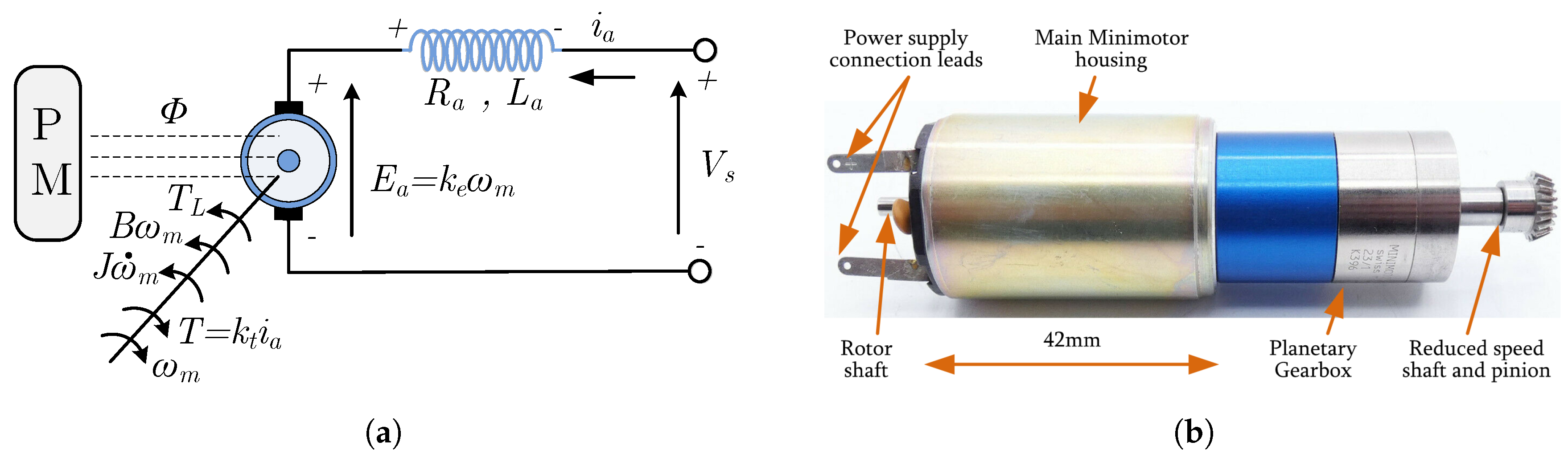
Figure 2.
Block diagram illustrating closed-loop architecture for DC micro-motor speed control.
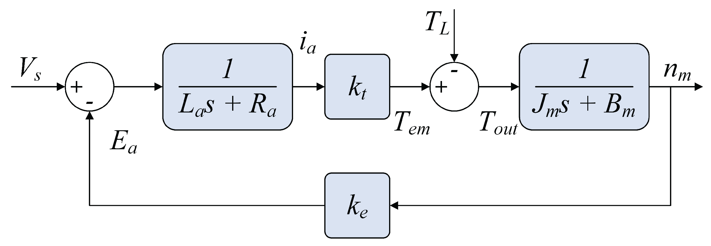
Figure 3.
Schematic of the negative feedback control loop for regulating DC micro-motor’s speed.
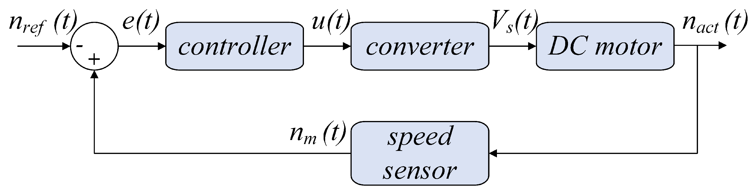
Figure 4.
Structure of the controllers under study: (a)PI (b) PID (c) PIDF.
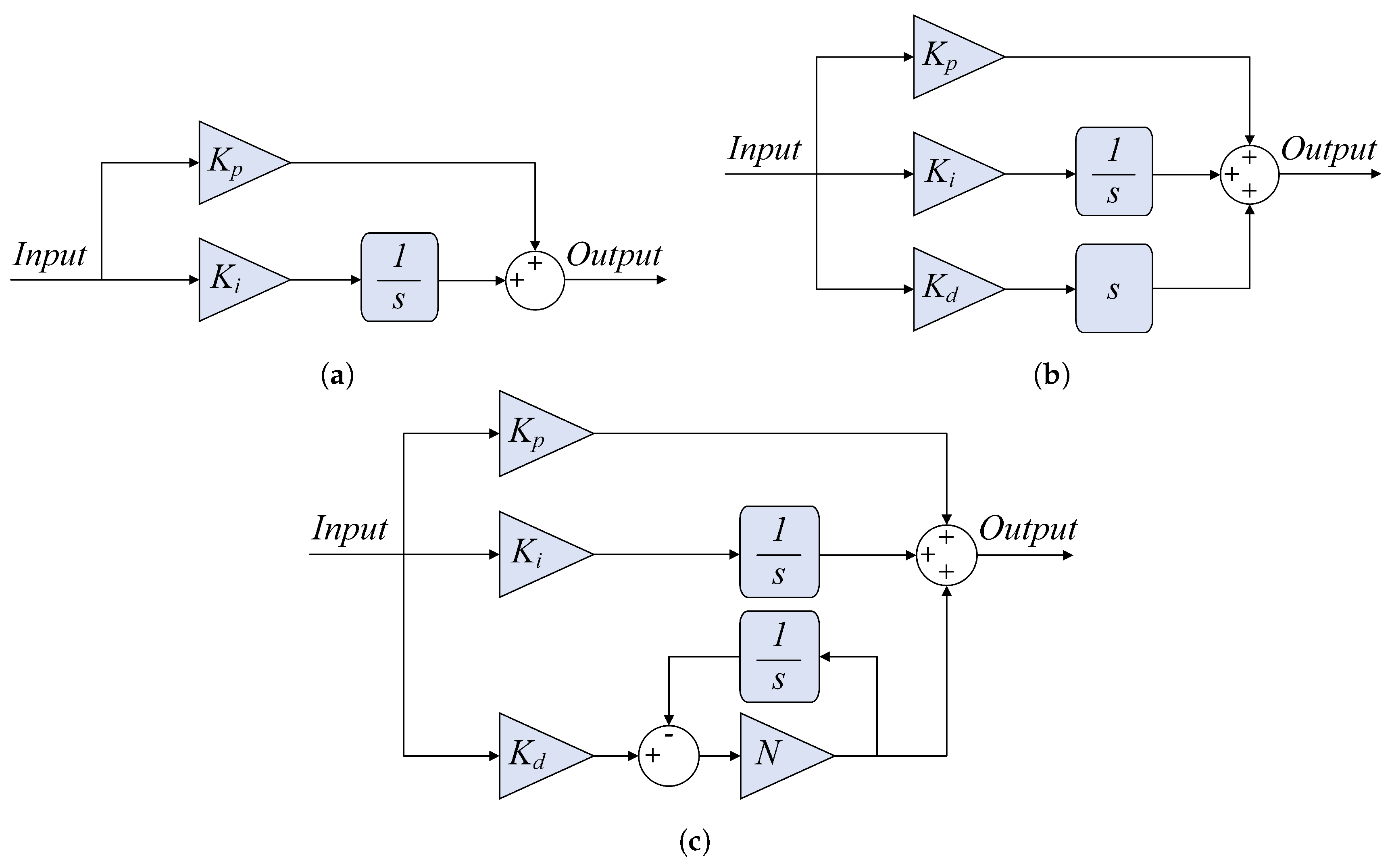
Figure 5.
Gaussian IT2 MFs with: (a) uncertainty in the mean (b) uncertainty in the standard deviation.
Figure 5.
Gaussian IT2 MFs with: (a) uncertainty in the mean (b) uncertainty in the standard deviation.
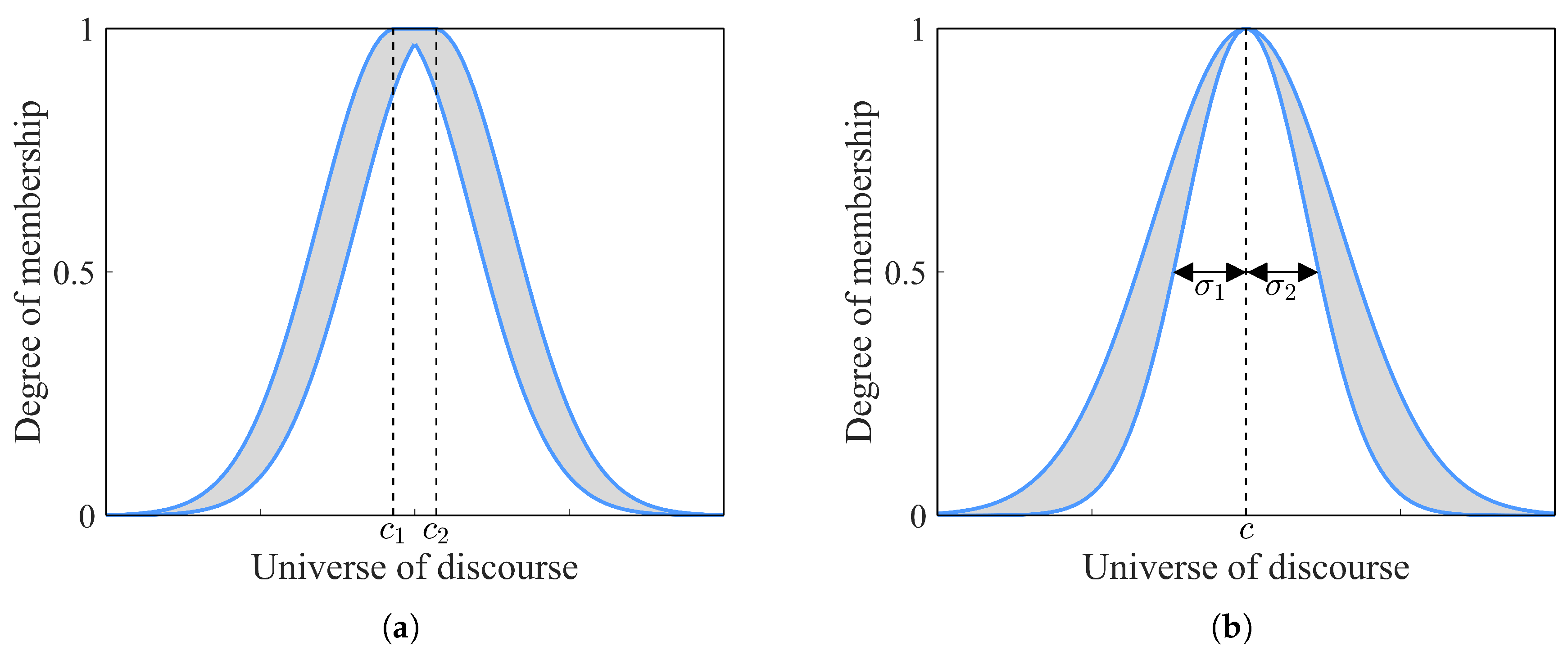
Figure 6.
Block diagram of the IT2-FLC structure.
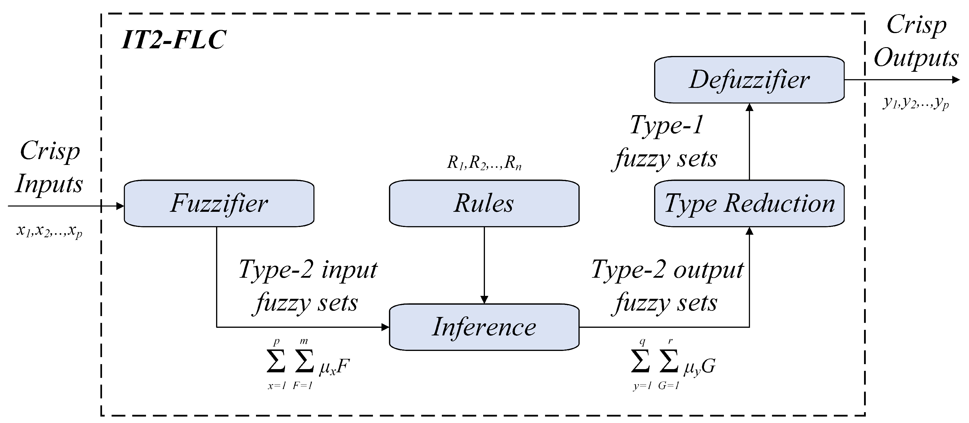
Figure 7.
Proposed IT2-PID controller structure.
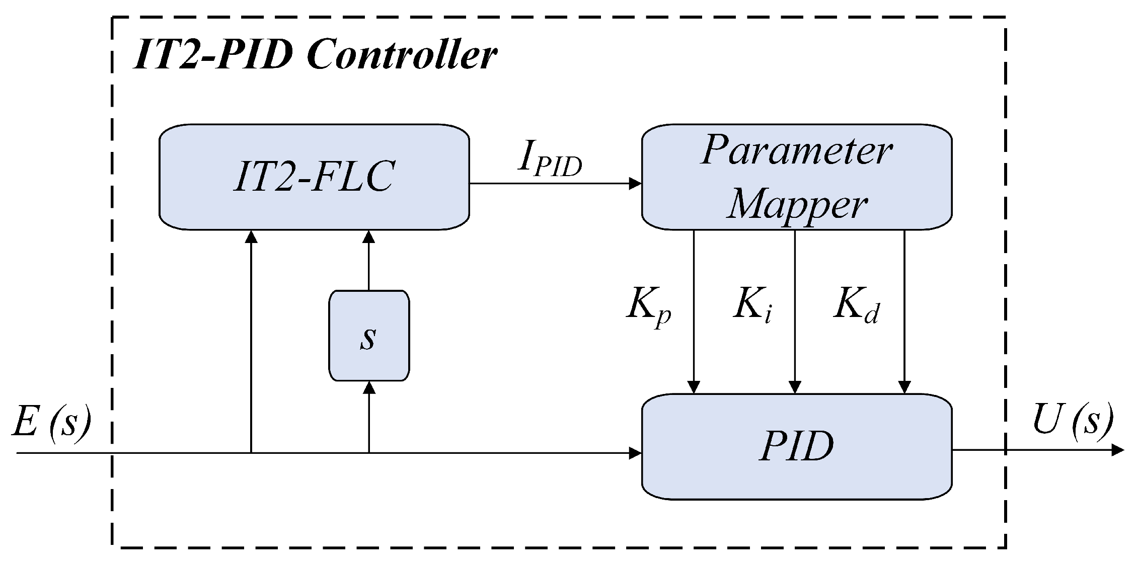
Figure 8.
Membership Functions of the IT2-FLC: (a) error, (b) change in error, (c) PID tuning index, and (d) the control surface of the inference system.
Figure 8.
Membership Functions of the IT2-FLC: (a) error, (b) change in error, (c) PID tuning index, and (d) the control surface of the inference system.
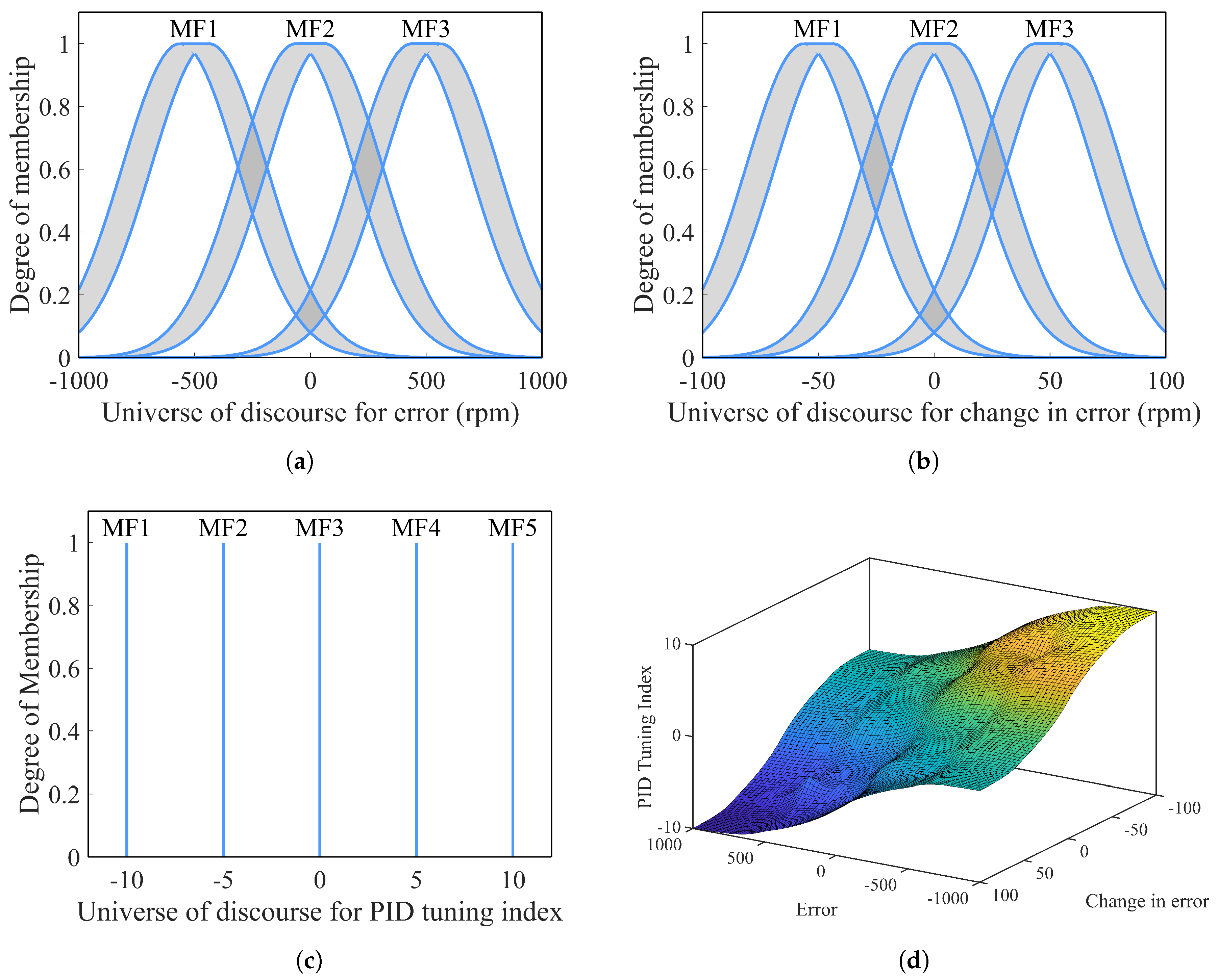
Figure 9.
Hardware Architecture Overview.
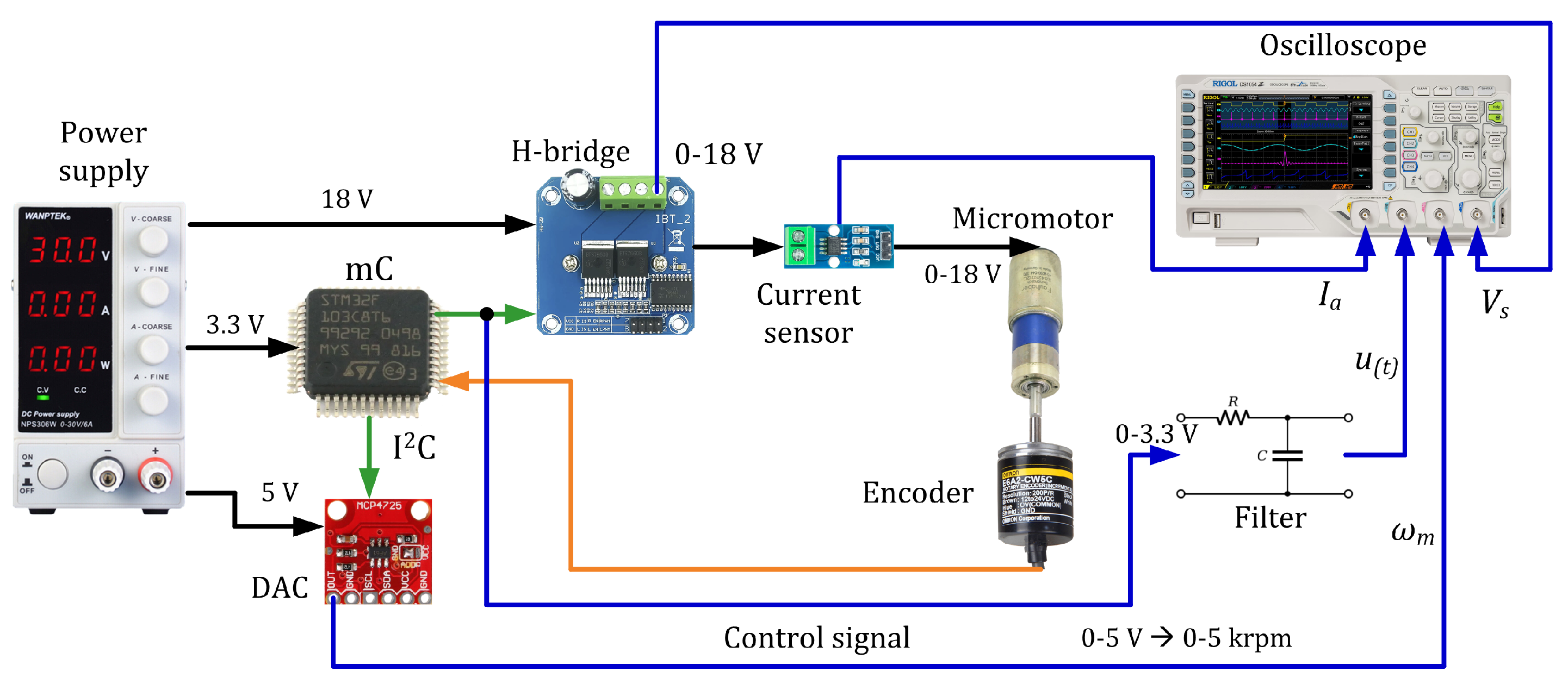
Figure 10.
Experimental testbench for DC micro-motor control and data acquisition.
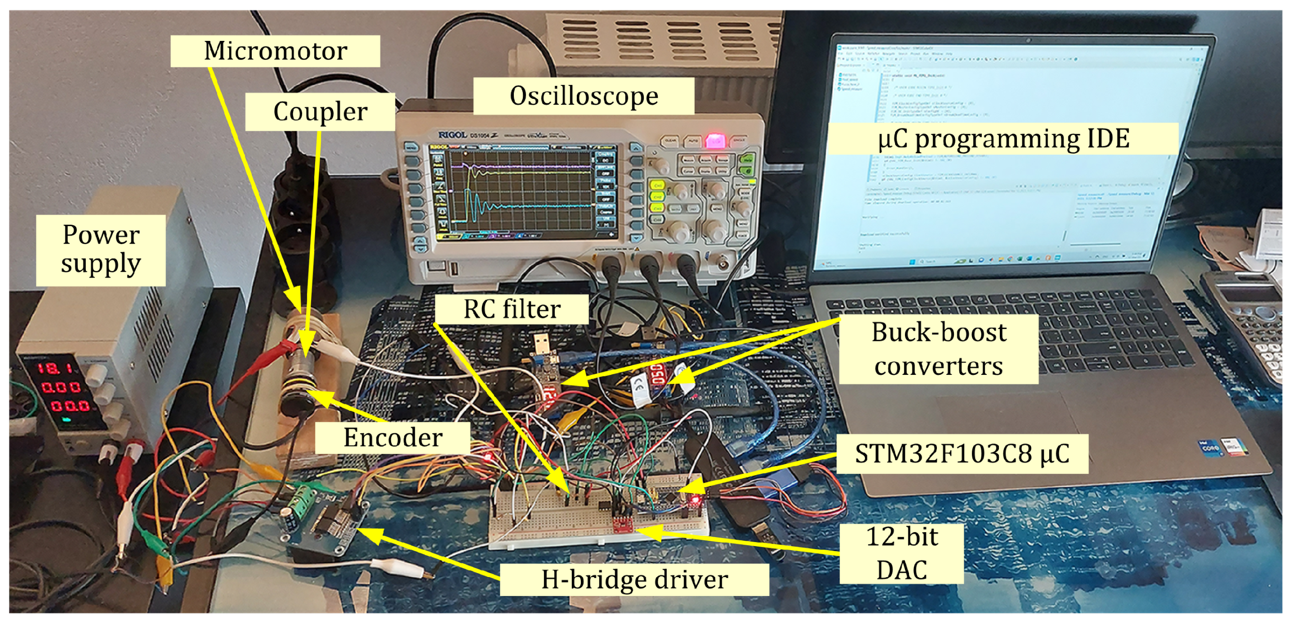
Figure 11.
Software architecture flowchart for (a) main control algorithm and (b) PSO tuning routine.
Figure 11.
Software architecture flowchart for (a) main control algorithm and (b) PSO tuning routine.
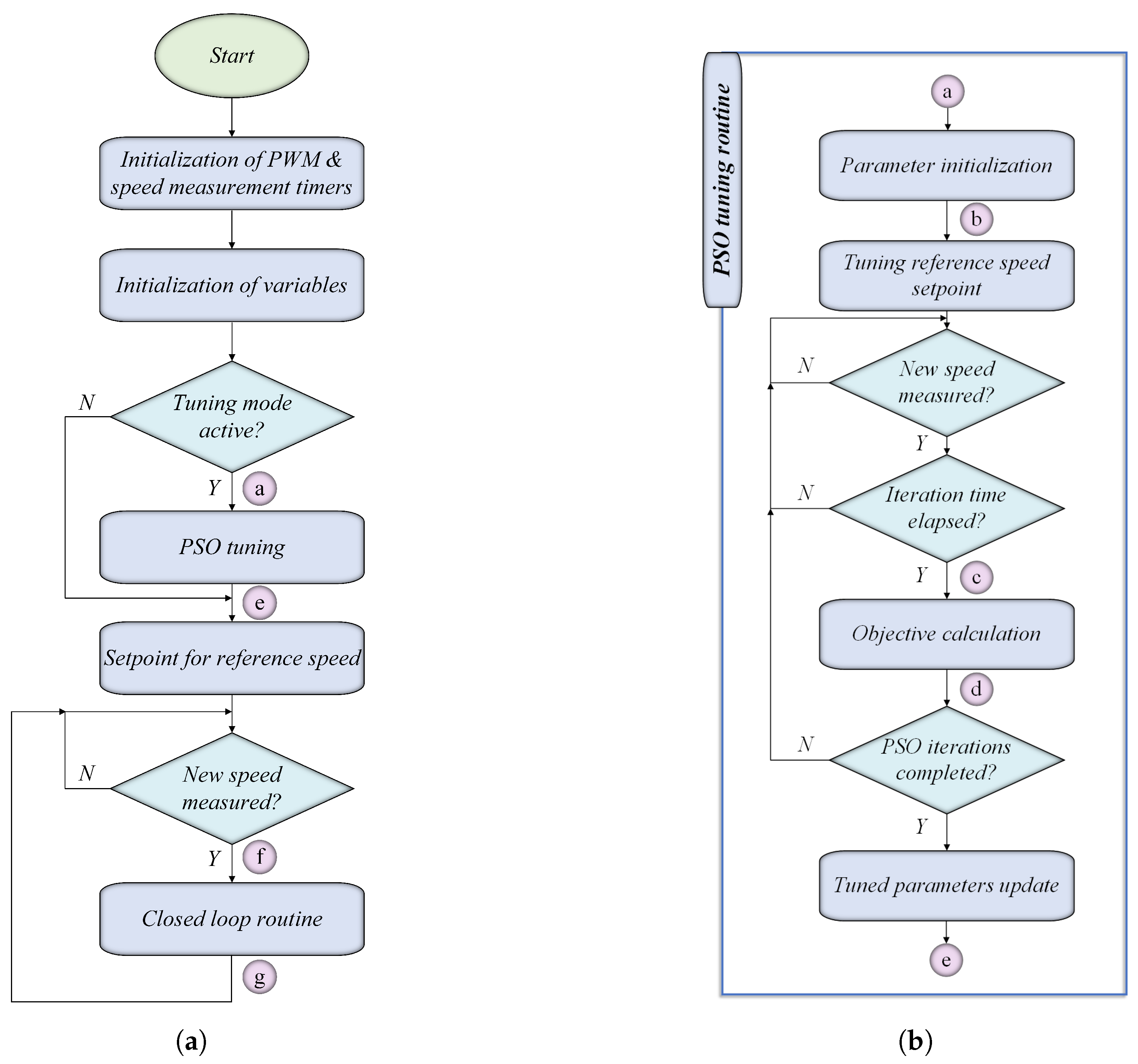
Figure 12.
PSO tuning subroutines (a) Parameter initialization and (b) Objective calculation.
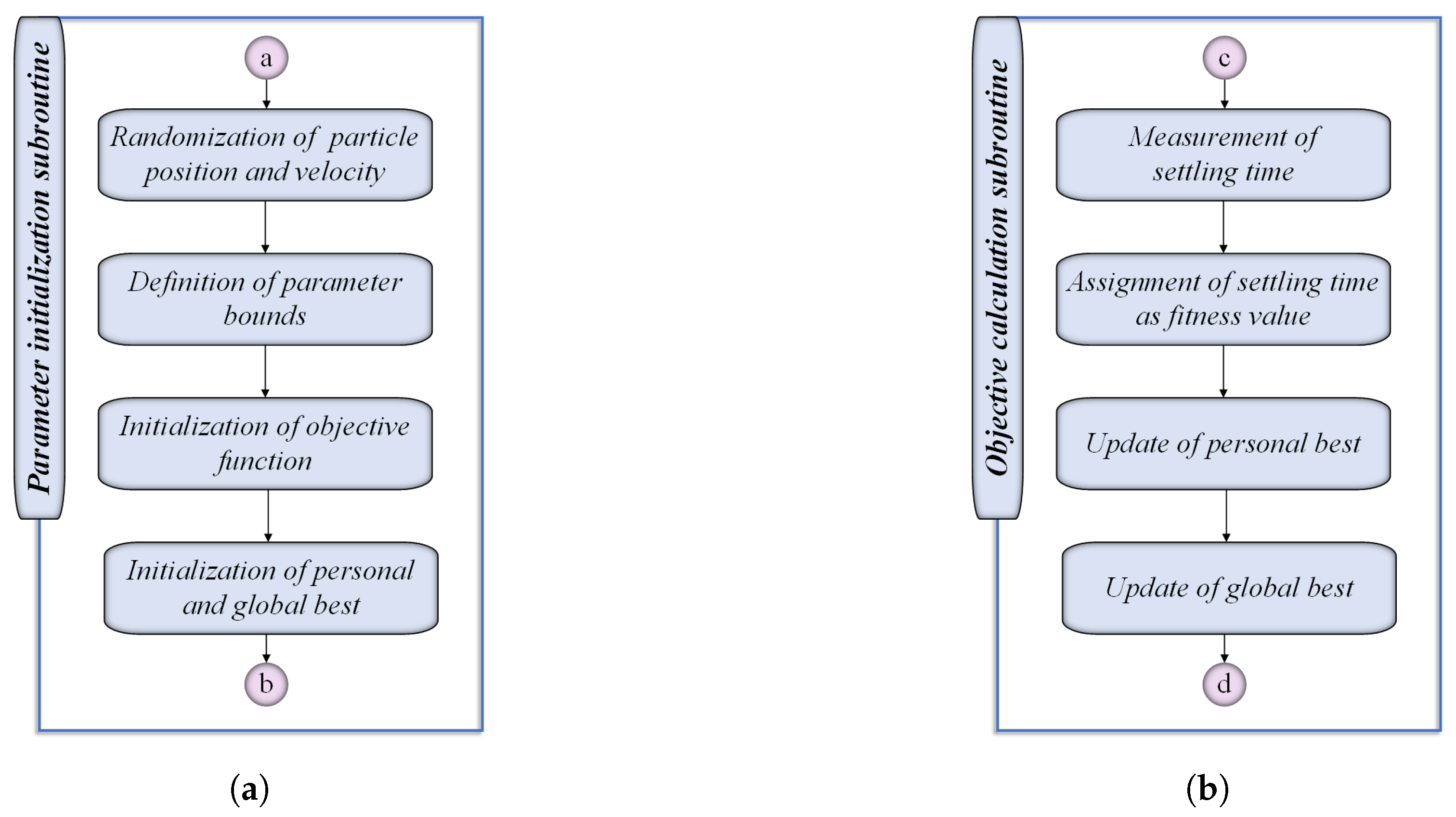
Figure 13.
Closed loop routine flowchart.
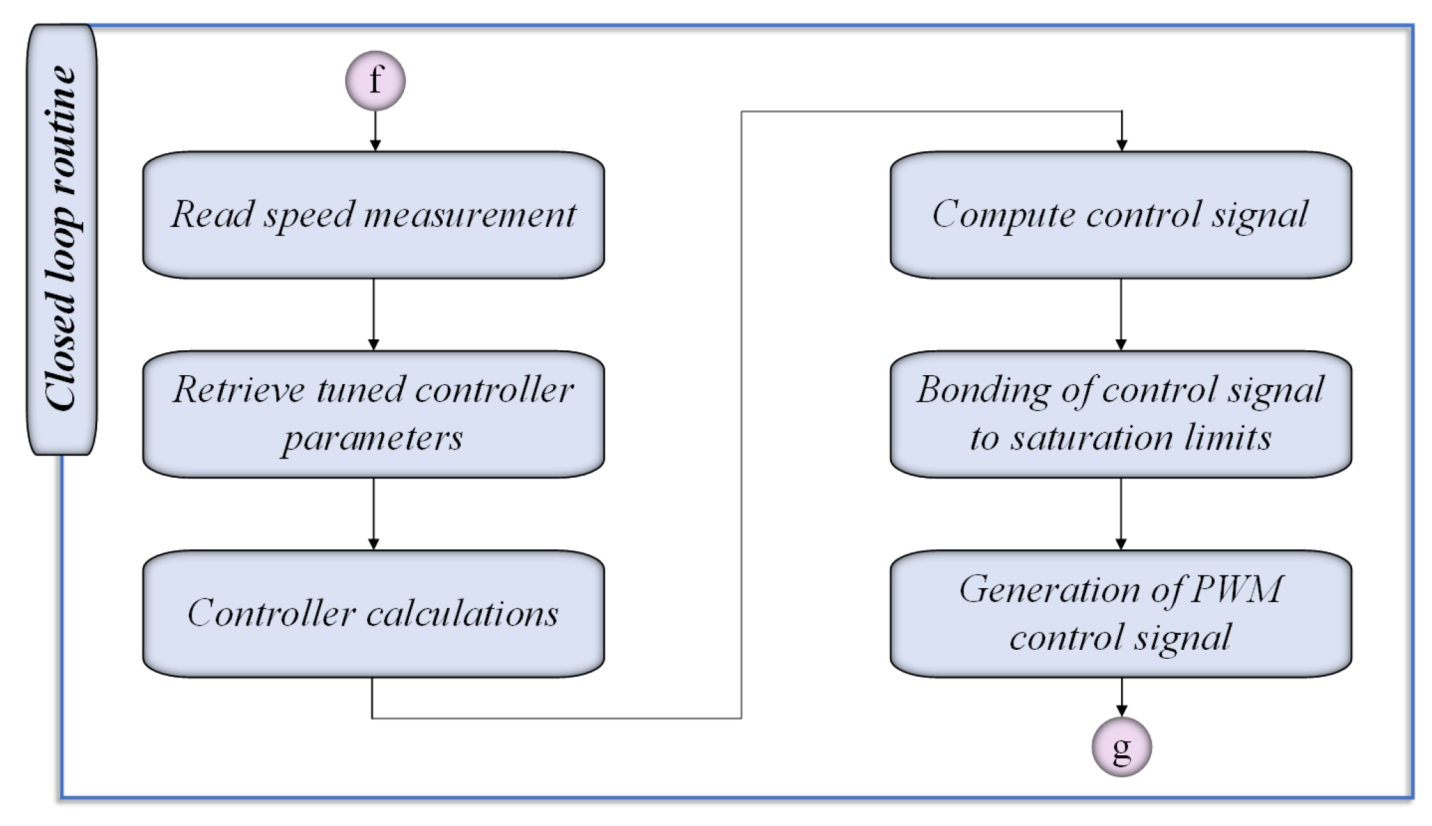
Figure 15.
Schematic of proposed speed measurement methodology.
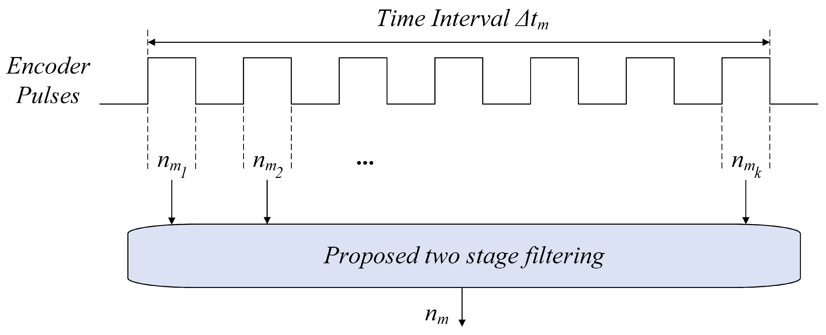
Figure 16.
Number of encoder pulses generated for different time intervals and micro-motor speeds.
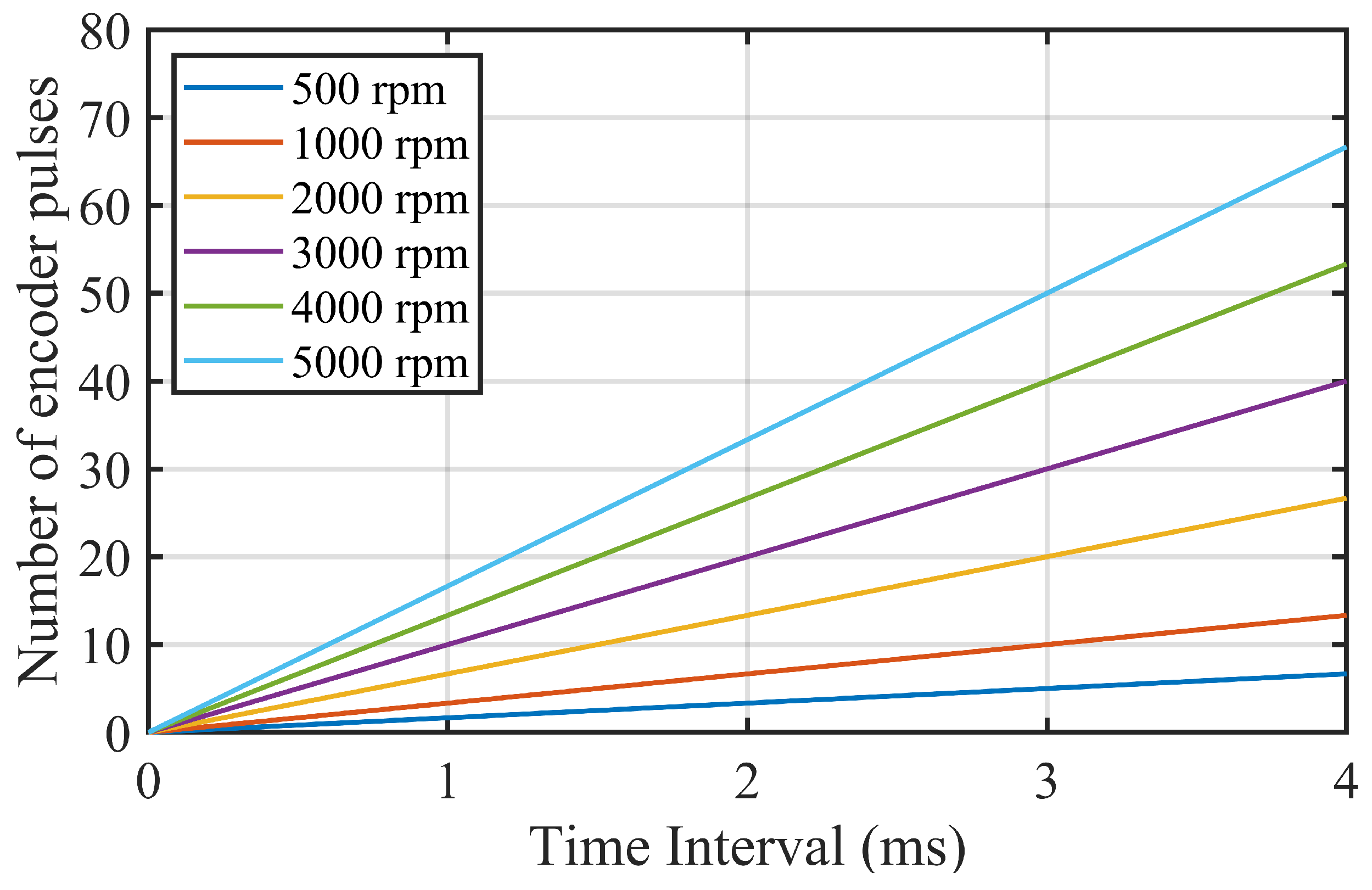
Figure 17.
Speed measurements for step voltage. (a) Comparison between raw data, Kalman filtering, and the proposed two-stage filtering method. (b) Depicts the step input voltage.
Figure 17.
Speed measurements for step voltage. (a) Comparison between raw data, Kalman filtering, and the proposed two-stage filtering method. (b) Depicts the step input voltage.
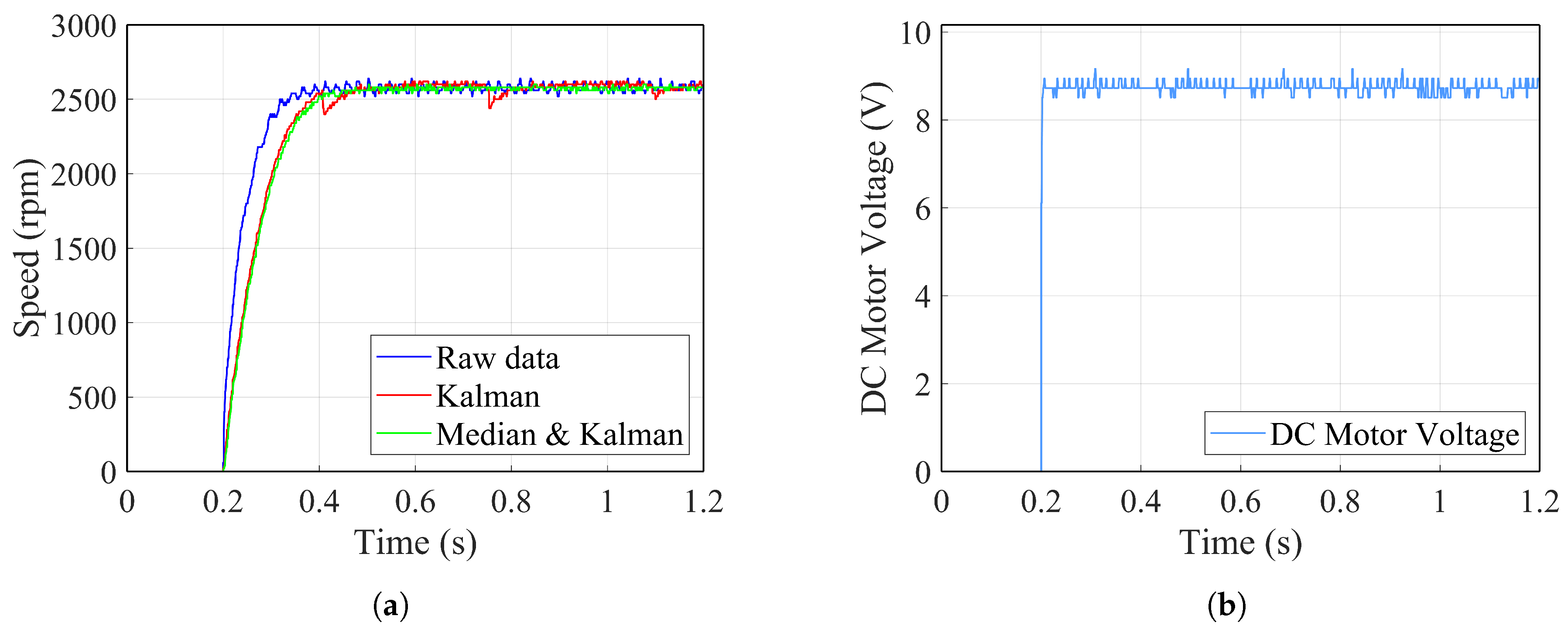
Figure 18.
PSO Convergence Times for Different Controllers. The plot illustrates the convergence times for PI, PID, PID with D Filtering (PIDF), and FT2-PID controllers. A target speed of 2750 rpm was maintained for all evaluations.
Figure 18.
PSO Convergence Times for Different Controllers. The plot illustrates the convergence times for PI, PID, PID with D Filtering (PIDF), and FT2-PID controllers. A target speed of 2750 rpm was maintained for all evaluations.
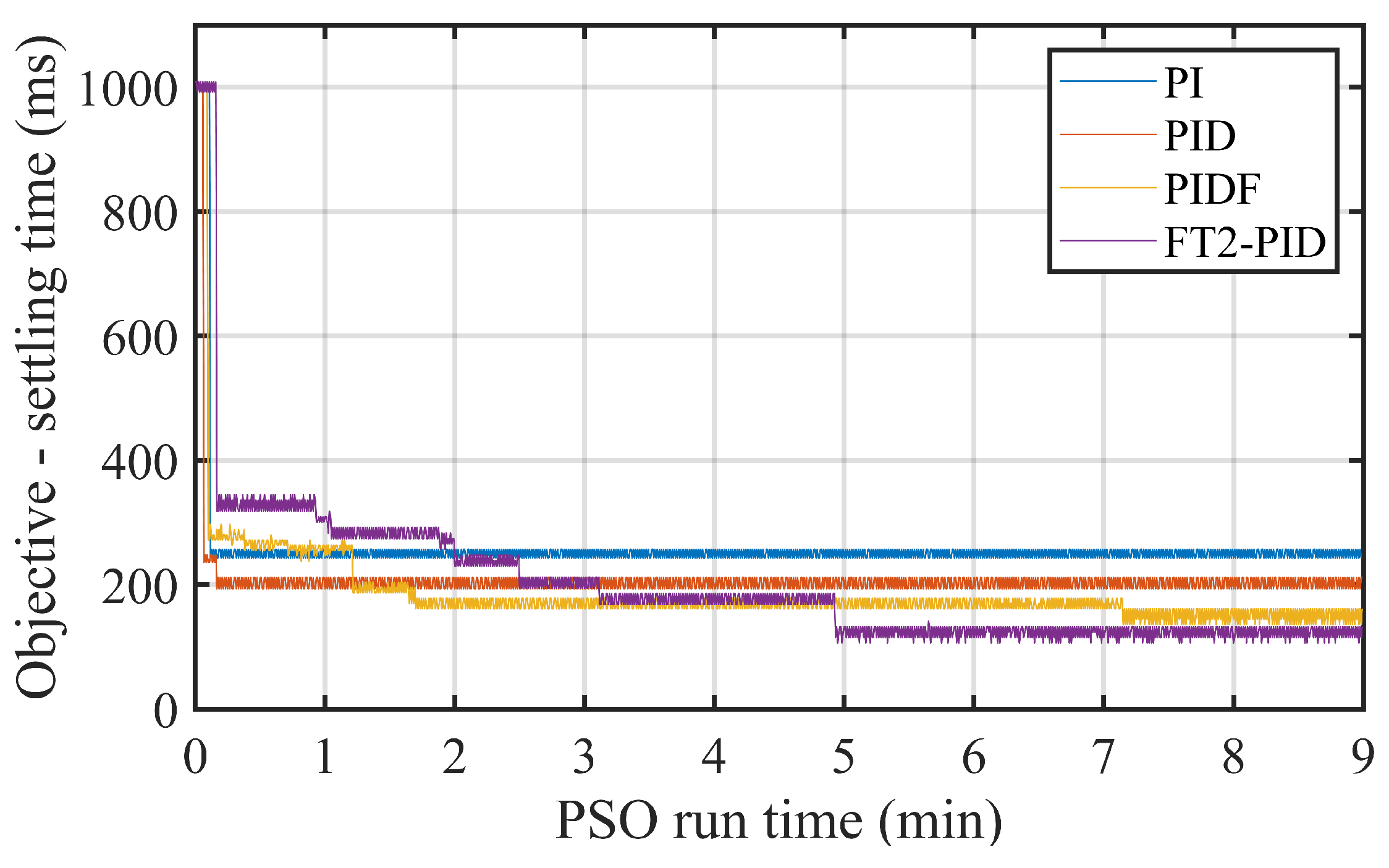
Figure 19.
Memory consumption comparison between SRAM and Flash for all controllers. (a) Shows SRAM memory consumption, and (b) shows Flash memory consumption.
Figure 19.
Memory consumption comparison between SRAM and Flash for all controllers. (a) Shows SRAM memory consumption, and (b) shows Flash memory consumption.
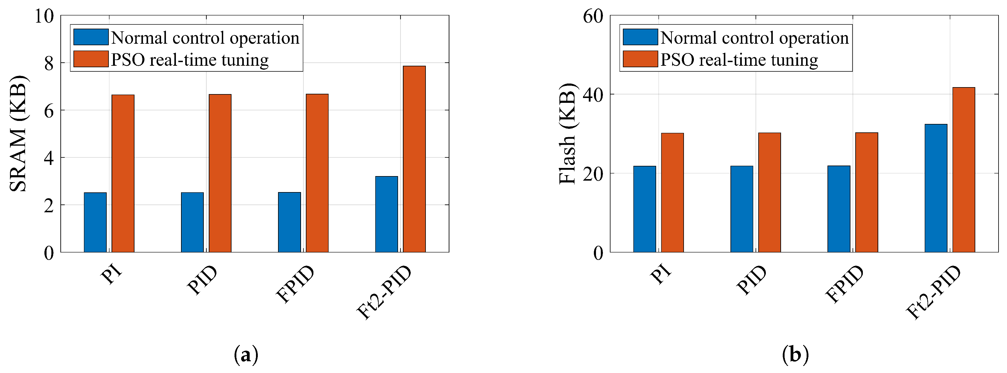
Figure 20.
CPU load for different steady state speeds.
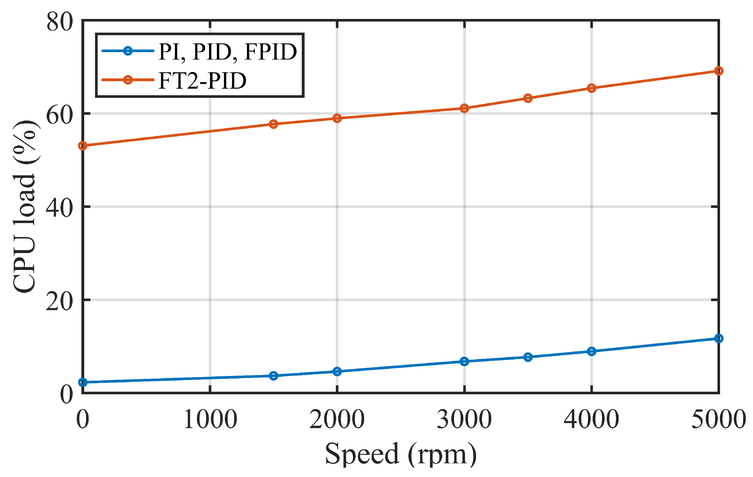
Figure 21.
Current experimental results for different reference speeds. (a) Shows the response for 2000 rpm, (b) for 2750 rpm, and (c) for 3500 rpm.
Figure 21.
Current experimental results for different reference speeds. (a) Shows the response for 2000 rpm, (b) for 2750 rpm, and (c) for 3500 rpm.
Figure 22.
Armature voltage experimental results for different reference speeds. (a) Shows the response for 2000 rpm, (b) for 2750 rpm, and (c) for 3500 rpm.
Figure 22.
Armature voltage experimental results for different reference speeds. (a) Shows the response for 2000 rpm, (b) for 2750 rpm, and (c) for 3500 rpm.
Figure 23.
Motor speed experimental results for different reference speeds. (a) Shows the response for 2000 rpm, (b) for 2750 rpm, and (c) for 3500 rpm.
Figure 23.
Motor speed experimental results for different reference speeds. (a) Shows the response for 2000 rpm, (b) for 2750 rpm, and (c) for 3500 rpm.
Table 1.
Advantages and disadvantages of filter coefficient value selection.
| N | Advantages | Disadvantages |
|---|---|---|
| Small | ✓ Fast response to rapid error changes. ✓ Better adaptation to dynamic error changes. ✓ Improved tracking of small error variations. | ✗ Limited noise suppression. ✗ Increased sensitivity to noise. ✗ Potential instability due to noise amplification. |
| Large | ✓ Enhanced noise filtering capabilities. ✓ Reduced controller impact of high-frequency noise. ✓ Improved stability by attenuating unwanted oscillations. | ✗ Slower response to fast error dynamics. ✗ Reduced system responsiveness to fast error changes. ✗ Possible increased overshoot and longer settling time. |
Table 2.
The developed Fuzzy Association Matrix (FAM) for IT2-FLC.
| Error | ||||
|---|---|---|---|---|
| MF1 | MF2 | MF3 | ||
| MF1 | MF5 | MF4 | MF3 | |
| Change in Error | MF2 | MF4 | MF3 | MF2 |
| MF3 | MF3 | MF2 | MF1 |
Table 3.
Parameter mapping based on PID Tuning Index.
| Corresponding PID Parameters | |
|---|---|
| [0, 1] | |
| (1, 2] | |
| (2, 3] | |
| (3, 4] | |
| (4, 5] | |
| (5, 6] | |
| (6, 7] | |
| (7, 8] | |
| (8, 9] | |
| (9, 10] |
Table 4.
Microcontroller specifications.
| Parameter | Details |
|---|---|
| Microcontroller | STM32F103C8 |
| Core Architecture | 32-bit ARM Cortex M3 |
| Clock Speed | 72 MHz |
| Operating Voltage | 3.3 V |
| Flash Memory | 64 KB |
| SRAM | 20 KB |
| Data Bus Width | 32 b |
| Cost | 5 € |
Table 5.
Summary of hardware components.
| Hardware | Part Number |
|---|---|
| Micro-motor | Faulhaber 2842S018C |
| Microcontroller | STM32F103C8 |
| Power supply | NPS306W |
| Oscilloscope | Rigol DS1054Z |
| Motor driver | BTS7960 |
| Speed sensor | OMRON E6A2-CW5C |
| Current Sensor | ACS712 |
| DAC | MCP4725 |
| Buck boost | DR-YM-288 |
Table 6.
PSO parameter values used in this work.
| Parameter | Value | Description |
|---|---|---|
| Population Size (N) | 6 | Particle population of the swarm. |
| Maximum Iterations () | 100 | Number of iterations. |
| Inertia Weight (w) | Varies between 0.2 and 0.9 | Exploration-exploitation balance. |
| Cognitive Coefficient () | 2 | Weight for the best personal position. |
| Social Coefficient () | 2 | Weight for the best global position. |
| Bounds for | [0, 10] | Proportional gain parameter range. |
| Bounds for | [0, 1] | Integral gain parameter range. |
| Bounds for | [0, 1] | Derivative gain parameter range. |
| Bounds for N | [0, 100] | Filter coefficient range. |
| Reference Speed Setpoint | 2750 rpm | Tuning micro-motor speed. |
Table 7.
Correlation between PWM resolution and frequency.
| Bit Resolution | PWM Frequency (Hz) |
|---|---|
| 10 | 70314 |
| 11 | 35156 |
| 12 | 17578 |
| 13 | 8789 |
| 14 | 4394 |
Table 8.
Advantages and disadvantages of selecting small or large .
| Advantages | Disadvantages | |
|---|---|---|
| Small | ✓ Enables faster control updates, improving response to dynamic changes. ✓ Facilitates frequent speed measurements, enhancing the precision of real-time control. ✓ Enhances the system’s capability to adapt to fast changes in speed. | ✗ Lower accuracy in speed estimation due to fewer encoder pulses within the interval. ✗ Increased sensitivity to signal noise, potentially introducing control instability. ✗ Limited low speed resolution, due to the small number of pulses produced within the time interval. |
| Large | ✓ Improves measurement accuracy by averaging over more encoder pulses. ✓ Provides smoother speed calculations with reduced sensitivity to noise. ✓ Increased resolution at low speeds since a higher number of pulses generated within the time interval. | ✗ Slower system response to dynamic changes, leading to potential prolonged error correction. ✗ Delays in control actions, potentially affecting performance in fast-changing scenarios. ✗ Increased likelihood of missing short-duration speed events. |
Table 9.
Selected Kalman filter parameters in this work.
| Parameter | Value |
|---|---|
| Process Noise Covariance (Q) | 0.0005 |
| Measurement Noise Covariance (R) | 0.1 |
| Initial Estimate Error Covariance (P) | 1 |
| Initial Speed Estimate () | 0 |
| Initial Kalman Gain (K) | 1 |
Table 10.
PSO tuning results for PI, PID, and PIDF controllers.
| Controller | N | |||
|---|---|---|---|---|
| PI | 4 | 0.12 | - | - |
| PID | 7.8 | 0.059 | 0.41 | - |
| PIDF | 2.72 | 0.0069 | 0.61 | 57.4 |
Table 11.
PSO tuning results for FT2-PID controller based on .
| [0, 1] | |||
| (1, 2] | |||
| (2, 3] | |||
| (3, 4] | |||
| (4, 5] | |||
| (5, 6] | |||
| (6, 7] | |||
| (7, 8] | |||
| (8, 9] | |||
| (9, 10] |
Table 12.
Memory requirements for DC micro-motor control.
| Memory | Total Size | PI | PID | PIDF | FT2-PID |
|---|---|---|---|---|---|
| SRAM | 20 KB | 2.51 KB | 2.52 KB | 2.53 KB | 3.20 KB |
| Flash | 64 KB | 21.78 KB | 21.84 KB | 21.88 KB | 32.39 KB |
Table 13.
Memory requirements for PSO real-time tuning.
| Memory | Total Size | PI | PID | PIDF | FT2-PID |
|---|---|---|---|---|---|
| SRAM | 20 KB | 6.64 KB | 6.66 KB | 6.67 KB | 7.86 KB |
| Flash | 64 KB | 30.14 KB | 30.22 KB | 30.28 KB | 41.69 KB |
Table 14.
CPU load at various micro-motor speeds.
| Speed (rpm) | CPU Load (% - PI, PID, PIDF) | CPU Load (% - FT2-PID) |
|---|---|---|
| 0 | 2.31 | 53.09 |
| 1500 | 3.70 | 57.72 |
| 2000 | 4.63 | 58.95 |
| 3000 | 6.79 | 61.11 |
| 3500 | 7.72 | 63.27 |
| 4000 | 8.95 | 65.43 |
| 5000 | 11.73 | 69.14 |
Table 15.
Overview of experimental cases and controllers.
| Case | Target Speed (rpm) | Controllers Evaluated | Objective |
|---|---|---|---|
| Case 1 | 2000 | PI, PID, PIDF, FT2-PID | Low-Speed Performance |
| Case 2 | 2750 | PI, PID, PIDF, FT2-PID | Mid-Speed Performance |
| Case 3 | 3500 | PI, PID, PIDF, FT2-PID | High-Speed Performance |
Table 16.
Rise time for examined controllers.
| Case | Reference Speed | PI | PID | PIDF | FT2-PID |
|---|---|---|---|---|---|
| 1 | 2000 rpm | 22.7 ms | 24.3 ms | 26.1 ms | 29.7 ms |
| 2 | 2750 rpm | 34.5 ms | 37.8 ms | 35.9 ms | 37.7 ms |
| 3 | 3500 rpm | 50.7 ms | 49.9 ms | 52.3 ms | 53.5 ms |
Table 17.
Overshoot for examined controllers.
| Case | Reference Speed | PI | PID | PIDF | FT2-PID |
|---|---|---|---|---|---|
| 1 | 2000 rpm | 19.00% | 14.00% | 9.00% | 12.00% |
| 2 | 2750 rpm | 21.00% | 11.00% | 11.00% | 12.30% |
| 3 | 3500 rpm | 25.00% | 8.00% | 16.00% | 12.50% |
Table 18.
Settling time for examined controllers.
| Case | Reference Speed | PI | PID | PIDF | FT2-PID |
|---|---|---|---|---|---|
| 1 | 2000 rpm | 240 ms | 230 ms | 145 ms | 104 ms |
| 2 | 2750 rpm | 250 ms | 203 ms | 149 ms | 123 ms |
| 3 | 3500 rpm | 313 ms | 245 ms | 225 ms | 167 ms |
Disclaimer/Publisher’s Note: The statements, opinions and data contained in all publications are solely those of the individual author(s) and contributor(s) and not of MDPI and/or the editor(s). MDPI and/or the editor(s) disclaim responsibility for any injury to people or property resulting from any ideas, methods, instructions or products referred to in the content. |
© 2025 by the authors. Licensee MDPI, Basel, Switzerland. This article is an open access article distributed under the terms and conditions of the Creative Commons Attribution (CC BY) license (https://creativecommons.org/licenses/by/4.0/).
Copyright: This open access article is published under a Creative Commons CC BY 4.0 license, which permit the free download, distribution, and reuse, provided that the author and preprint are cited in any reuse.


