
Submitted:
03 March 2025
Posted:
04 March 2025
You are already at the latest version
Abstract
This paper presents the design, implementation, and experimental validation of a switched SW FOPID-PID controller for the stabilization of an inverted pendulum (InvP) system. Additional PID and Fractional Order PID (FOPID) controllers were also designed, tuned and validated for comparison purposes. The controllers were tuned offline using Particle Swarm Optimization (PSO) and a mathematical model of the system for simulation. Their performance was assessed through key indicators, including ITAE, ISI, settling time, peak values, and variance, and compared against a manufacturer-provided PID controller. Experimental results demonstrated that all three designed controllers outperformed the manufacturer’s PID under nominal conditions. The SW FOPID-PID controller achieved the best overall performance, balancing control energy efficiency and response quality. Under external disturbances, the FOPID and SW FOPID-PID controllers exhibited superior robustness, being the switched controller the most effective, responding quickly to disturbances while minimizing positional and angular errors.
Keywords:
Switched Fractional Order PID
; Particle Swarm Optimization
; Control energy
1. Introduction
In the constant search for control strategies that yield better results than those currently available, it is essential to address the question: Better in what aspect? Frequently, the effectiveness of the controlled system, assessed through performance indicators, is crucial in responding to this question. Nevertheless, other factors such as the efficient use of control energy, the simplicity or complexity of the controller tuning process, the cost of developing the controller, and its implementation, among others, can also be taken into account.
Despite all the advancements in new control strategies, the most widely used controller remains the Proportional Integral Derivative (PID) controller. It is often preferred due to its simple structure and because its tuning and implementation tend to be simpler than most other controllers. A relatively straightforward alternative to the PID is its fractional-order counterpart, the FOPID, where the integral and derivative components can be of non-integer orders. The fractional-order PID controller (FOPID) is notable for its reduced sensitivity to parameter changes [1] and noise [2,3], better disturbance rejection [1], improvements in transient response [4], and an increased range of gains that ensure stability [5,6,7,8], among other benefits. Additionally, smoother control signals have been reported, which are associated with lower control energy consumption [1,5,9,10,11].
However, these advantages often come at the cost of slower error convergence compared to the use of PID, deteriorating key performance indicators. The PID, in contrast, can provide an effective response in terms of convergence speed when the system’s complexity is manageable, although this typically requires higher control energy [12]. In certain applications, the FOPID might achieve improved performance, while the PID may utilize lower control energy [13], but this trade-off is usually evident.
To address this trade-off, a viable alternative could be a switched control scheme, SW FOPID-PID, which essentially allows for switching between a PID and a FOPID according to a specific switching rule. The aim is to leverage the best characteristics of each controller while minimizing their individual shortcomings compared to their non-switched equivalents. This means that system performance optimization relies on the careful selection of the switching criterion between schemes, as well as the parameters of each controller.
Validation of new controllers, such as the mentioned SW FOPID-PID, is often conducted using simulated models, primarily because of the high costs associated with owning experimental plants. Nevertheless, experimental validation is preferred within the control community since it enables testing new controllers in realistic scenarios. The inverted pendulum system (InvP), known for its highly nonlinear dynamics, serves as an ideal and widely used test model for designing and validating new control strategies. Its applications cover various engineering problems due to its similarities, particularly in rocket launching, robotic arm control, and self-balancing vehicles [10,14], among others. The main control challenge is to stabilize the pendulum in its upward vertical position, although a pendulum lifting process must be completed before reaching this stage.
In technical literature, several works report the experimental validation of FOPID controllers in the InvP system, often compared to the classic PID controller. For instance, see [14,15,16,17,18,19,20]. However, to the authors’ knowledge, no studies have been reported on the experimental validation of SW FOPID-PID controllers in the InvP system.
For a system different from the InvP, three works have been identified that provide some experimental validation of a switched SW FOPID-PID. The first study is [21], which applies a switched Fractional Order Proportional Integral Controller (SFOPI) to regulate the DC link voltage of a single-phase active power filter under unbalanced conditions. The authors state that the classic PI offers better steady-state behavior but is limited during the transient stage, while FOPI addresses this transient drawback but leads to significant degradation in control performance during steady state. Consequently, the authors propose a switching controller that alternates between the PI and the FOPI, using the absolute value of the control error as the switching decision variable. The controller underwent experimental testing, and the results were compared with standard PI and sliding mode controllers, demonstrating improvements in settling time and overshoot. The same authors improved the controller performance in [22] by modifying the switching mechanism with a fuzzy logic supervisor. Later, almost the same group of authors presented another application of the SFOPI in [23,24], this time focusing on the control of a grid-connected Wind Energy Conversion System, where the same advantages were noted. Although these two works provide some experimental validation (none targeting the InvP system), it should be noted that the controlled system is modeled as a linear system and the controller is designed based on those constraints. Additionally, the validated controller is a SFOPI, which lacks the fractional derivative component, known to pose an additional challenge for experimental validation. Furthermore, no analysis is conducted on the balance between control energy and system performance in the context of the switched approach.
The third work reporting the validation of certain switched SW FOPID-PID controllers is referenced in [13], where a SFOPI controller is designed and experimentally validated for level control in a conical tank. In [13], although the system is nonlinear and its nonlinear model is used for controller design and tuning, its equilibrium point is stable, which is not the main challenge in validating a controller, unlike the situation with the InvP system, whose equilibrium point is highly unstable. While the resulting control energy is discussed and analyzed in this work, the controller also lacks the fractional derivative component.
This work addresses the challenge of designing and tuning a switched controller, SW FOPID-PID, to stabilize an inverted pendulum system (InvP), along with its corresponding experimental validation. The primary goal of this control strategy is to ensure a better balance between control energy consumption and various performance indicators, and the experimental validation in this complex scenario represents a significant contribution of this research.
In the following, Section 2 will present the concepts used in the paper along with the description and mathematical model of the InvP. Section 3 introduces the controller design and tuning, while Section 4 presents the results and discussion of the experimental validation. Finally, Section 5 summarizes the main conclusions of the work.
2. Preliminaries
This section includes concepts and definitions utilized throughout the paper, as well as the system description and mathematical model employed for controller tuning purposes.
2.1. Fractional calculus
Fractional operators are integrals and derivatives of orders that can be real or complex numbers [25]. The fractional integral of a function is defined by [26] as
where , is the gamma function and . In the frequency domain, the Laplace transform of the fractional integral of order is given by [25].
This paper uses the Caputo fractional derivative, which is defined as
In the frequency domain, the Laplace transform of the Caputo fractional derivative of order corresponds to [25].
2.2. Fractional order proportional integral derivative controllers
FOPIDs are a generalized version of PID controllers in which the integral and derivative of the control error can be of real order. In the frequency domain, the expression relating the input and output of the FOPID controller (transfer function) corresponds to
where is the Laplace transform of the control signal, is the Laplace transform of the control error, , and are the proportional gain, integral gain and derivative gain, respectively, is the fractional integration order and is the fractional derivation order. It can be observed that the classic PID controller is a particular case of (3), when .
2.3. Inverted Pendulum system description
The system to be controlled in this work corresponds to an Inverted Pendulum (InvP) system, manufactured by Feedback Instruments Ltd. Figure 1 shows a picture of the plant in the research group laboratory.
A general diagram of this system, provided by the manufacturer, can be seen in Figure 2. The InvP system can be divided into three main components: the mechanical unit, the DC motor & interface unit, and the communication system.
The mechanical unit of the InvP includes all the mechanical elements of the system and essentially consists of a cart with two pendulums traveling on a rail [27]. The mechanical unit features a rail fixed to a base supported by two adjustable legs, allowing the rail to remain level. As illustrated in Figure 3, a direct current (DC) motor is positioned at one end of the rail, driving a sprocket wheel that, when in motion, moves a plastic toothed belt. This belt extends to the opposite end of the rail, where another sprocket wheel helps maintain its tension before it returns to the motor’s end. A metal cart is connected to the plastic belt along the rail. A metal shaft in the center of the cart links two pendulums with mass at their longer ends, which can rotate freely. The movement of the cart is caused by the DC motor at the end of the rail, pulling the belt in two directions. By applying voltage to the motor, the force with which the cart is pulled can be controlled. The force value is dependent on the control voltage applied to the motor, which rotates at a velocity proportional to the control voltage applied.
Both the cart’s shaft and the DC motor are equipped with optical encoders, enabling the measurement of the cart’s relative position as well as the pendulum’s relative angular position. An optical encoder comprises a light source, a light detector, and a slit disk positioned between them. This setup allows the measurement of relative position with respect to the initial point by counting the pulses detected by the light detector [27]. To obtain accurate data, the cart must be centered on the rail before any tests are conducted, and the pendulum should rest in the lower (hanging) position. These positions are defined as 0 [m] for the cart’s position and [rad] for the pendulum’s angular position, respectively. The cart can move freely along the rail, up to 1 [m] from the center in both directions. At these points, limit switches will activate if the cart reaches these positions, causing the DC motor to stop for safety reasons. Conversely, the pendulum can move across its full range from 0 [rad] to [rad].
The DC motor and interface unit is responsible for receiving position signals from the optical sensors located in the mechanical unit and transmitting them to the computer, where control algorithms will run. Similarly, it receives the control signal from the computer, which is a voltage ranging from [V] to [V], and sends it to the DC motor, which is also powered through this unit. Additionally, this unit executes the emergency stop if a limit switch is activated. It also features two buttons: a green button that allows tests to be conducted (enabling the inverted pendulum system for experiments) and a red button that serves as a manual emergency stop.
The communication system comprises two fundamental components: a Small Computer System Interface (SCSI) adapter and a data acquisition card, specifically the Advantech PCI-1711U-CE. The SCSI adapter enables data and signal transmission between the computer and the mechanical unit, allowing real-time monitoring and control. The Advantech PCI-1711U-CE data acquisition card allows real-time data acquisition, essential for monitoring and controlling the system, and communicates with the computer via a Peripheral Component Interconnect (PCI) port. This card includes 16 analog input channels, two 12-bit analog output channels, 16 digital input channels, 16 digital output channels, a programmable counter, and a 12-bit Analog/Digital (A/D) converter with a sampling rate of up to 100 [kHz] [27]. Figure 4 illustrates the connection diagram between all the elements.
2.4. Mathematical model of the plant
To simulate the system, as well as to design, tune, and validate controllers for it, obtaining a sufficiently representative mathematical model of the system to be controlled is necessary. In the case of the InvP system, both the cart-pendulum and the DC motor must be modeled.
In the case of the cart-pendulum system, the manufacturer provides a nonlinear model as follows [27]
where x [m] is the cart position with respect to the center of the rail, [rad] is the pendulum angular position with respect to the vertical, g is the gravitational acceleration, l is the pendulum length, M is the mass of the cart, m is the mass of the pendulum, I is the moment of inertia, b is the friction coefficient of the cart, d is the viscous friction coefficient of the pendulum, and F is the force applied to the cart by the motor and the input to the system. The numerical values of the eight specified parameters are listed in Table 1.
Although the manufacturer’s manual [27] provides only these nonlinear equations, they can be derived by defining kinetic energy and potential energy, forming the Lagrangian, and obtaining the Lagrange equations for both the cart position (x) and the pendulum angular position (). Details of this derivation are not included in this manuscript due to space constraints, but they can be found in [28].
Regarding the DC motor, it can be modeled as a resistor R in series with an inductance L, along with a voltage opposing the source (back electromotive force), which is generated by the motor’s angular velocity. Using Kirchhoff’s voltage law [29] and the rotational dynamics of the motor along with Newton’s second law, the following equations can be derived to describe the DC motor dynamics
where i [A] is the current, v [V] is the source voltage, [rad/s] is the angular velocity, J is the inertial constant, B is the inertial moment with respect to the motor center of mass, is the electromotive constant, is the torque constant, R is the electrical resistance, and L is the electrical inductance. Numerical values of the six specified parameters can be found in Table 1.
Since the DC motor model must be coupled with the cart-pendulum model, it is necessary to establish the mathematical relationship between the DC motor variables and the force F applied to the cart. In order to do this, the current-torque relationship and the torque-force relationship are used, both of which are included in the simulation software provided by the plant manufacturer [27] as follows
where is the motor torque.
Once the representative mathematical models of the cart-pendulum and DC motor are obtained, they are programmed in a computational environment. In this case, Matlab/Simulink is utilized, which is intuitive for modeling, simulating, and analyzing dynamic systems. Figure 5 illustrates a block diagram depicting the programmed structure. As shown in Figure 5, the input to the system corresponds to the voltage applied to the DC motor v, while the outputs are the pendulum’s angular position and the cart’s position x.
In Matlab/Simulink, the DC motor equations (6), (7), (8) are programmed into one block (DC motor block in Figure 5), whose input is the voltage applied to the motor, v, and the output is the force, F, applied to the cart. A second block (the one with the cart-pendulum in Figure 5) is then connected in series with the first block, which incorporates the nonlinear equations 4 and 5. This second block takes the force F as its input and produces the pendulum’s angular position, , and the cart’s position, x, as outputs.
3. Controllers Design and Tuning
The inverted pendulum control task can be seen as a self-erecting control problem, which is present in missile launching and control applications, to stabilize the inverted pendulum in an upright position. The inverted pendulum is inherently unstable. Left without a stabilizing controller, it will not be able to remain in an upright position when disturbed.
3.1. Controllers Included in the InvP System by Manufacturer
The inverted pendulum control provided by the manufacturer is divided into two distinct control problems. The first is the swing-up control, which enables the pendulum to reach the upright position (around ) [rad]. The second involves controlling around that equilibrium point, which is achieved using PID control [27].
In the case of the swing-up control, the goal of the control is to bring the pendulum to an upright position with as minimal angular velocity as possible. This will ensure that the stabilizing controller, which takes over from the swing-up controller, will have an easy task. A large velocity value at the point of controller changeover could cause the pendulum to over swing or cause very nervous reactions of the cart or even cause it to hit the end of the track [27].
If the acceleration is unbounded, it is possible to bring the pendulum to the upright position in a single swing. However, because of safety it is better to swing up the pendulum in a robust way, which will assure that the pendulum will end up in a vertical position where . The motor control signal is bounded to [V] (the actual range is 0 [V] to [V]) and [N] in terms of force, so these are the maximal values that can be transferred. The physical bound of the track has also to be considered [27].
There are many algorithms used for swing-up control; however, their robustness is in trade-off with their time performance. The manufacturer provides one strategy that achieves the control goal by using a set of rules to define the control signal. Since the aim of this work is to propose controllers for the stabilization stage, the swing-up control provided by the manufacturer will be used without modifications.
For the stabilization stage, which is the main goal of this work, manufacturer provides a PID controller. Since the inverted pendulum is a Single Input Multiple Output (SIMO) system, two separate PID controllers are provided (one for angular position and one for cart position x), and their outputs are combined to generate the final single control signal, as can be observed in the block diagram of Figure 6.
According to Figure 6 and the manufacturer manual, the control signal in the Laplace domain will be defined as
where , , and are the proportional gain, integral gain, and derivative gain, respectively, of the PID controller for angular position. On the other hand, , , and denote the proportional gain, integral gain, and derivative gain, respectively, of the PID controller for the cart’s position. The control error for the cart’s position is expressed as , while represents the error in the pendulum’s angular position, where and are the reference signals for the angular position of the pendulum and the position of the cart, respectively. Since the goal is to center the cart on the rail and maintain the pendulum in a stable upright vertical position, both the reference for the cart position and the reference for the pendulum’s angular position are set to zero. The manufacturer provides the numerical values of the controller gains as shown in Table 2. In the following sections, this controller will be referred to as .
3.2. Design of switched fractional order proportional integral derivative controller
A different tuning for PID controllers or the design and tuning of FOPID controllers could lead to improvements in control energy and system performance, compared to . However, these controllers can present a sort of trade-off between control energy and system performance, thus leading to the idea of using a switched version of them, trying to combine the strengths of both controllers. In the particular case of the inverted pendulum (PInv), the block diagram of the proposed strategy can be seen in Figure 7.
A switching mechanism will allow alternating between a PID and FOPID controller, based on a criterion which in this case depends on the control error for the angular position . Specifically, the FOPID control signal will be sent to the plant when the absolute value of the angular position control error exceeds a certain threshold (design parameter), while the PID control signal will be sent when it is below this threshold. This means that the FOPID controllers would operate during transients and disturbed stages, providing their corresponding advantages, and the PID controllers would mostly operate near the steady state, offering their advantages of fast convergence. The equation representing the switched control scheme is therefore defined as follows
where corresponds to the absolute value of the control error of the pendulum’s angular position , is a design parameter, is defined as in (9) and is defined in the Laplace domain as
with , and the proportional gain, integral gain and derivative gain, respectively, of the FOPID controller for the angular position, while and are the fractional orders for the integral part and the derivative part, respectively. On the other hand, , , and are the proportional gain, the integral gain, and the derivative gain, respectively, of the FOPID controller for the position of the cart, while and are the fractional orders of the integral and derivative parts of this controller, respectively.
To implement the switched control scheme, it was decided to filter the control signal v (as shown in Figure 7) to smooth it before injecting it into the system. This is necessary because switching between control schemes can lead to abrupt transitions, which should be avoided for actuator protection. The filter used is a first-order transfer function defined by
where s represents the complex variable in the Laplace domain, and is the time constant. As shown in (12), incorporating this filter into the control scheme adds a pole to the system, which remains stable for any positive value of . The time constant adjusts the speed of the filter’s response. A smaller value of enables the filter to pass higher frequency signals, resulting in a faster response but with a less smoothing effect on transitions. On the other hand, a larger value of will provide a higher smoothing effect but may introduce a delay in the system’s response. Therefore, there is a trade-off between smoothing and delay, so the process of selecting the time constant must be done carefully. For simulation purposes and controller tuning, a value of was established and maintained in experimental tests. The tuning process was conducted through trial and error.
3.3. Tuning of controller parameters
According to the structure of the switched controller proposed in Section 3.2, the number of parameters to be tuned using the optimization process is 17, of which 6 correspond to the PID controllers, 10 correspond to the FOPID controllers, and the last one corresponds to the threshold value , which is compared to the absolute value of the error to determine when to switch. The parameter vector to be adjusted is therefore defined as follows:
where the subscript f in the gains refers to the FOPID controller.
Due to the large amount of controller parameters to be tuned, an offline optimization process was conducted, specifically using Particle Swarm Optimization (PSO) and using the mathematical model of the system for simulation purposes.
Before starting the controller tuning process with an optimization algorithm, it is essential to establish the criteria that the algorithm will use to evaluate and refine the design parameters. To achieve this, the system’s performance is assessed according to two criteria: the performance of the controlled system and the use of control energy. These performance indices will also facilitate conclusions about the impact of the design parameters and the pros and cons of the resulting controllers during a later results comparison.
The performance of the controlled system is evaluated through the integral of the time-weighted absolute error (ITAE), which is given by
where corresponds to the simulation/operation time of the controlled system at the time of controller tuning, and e to the control error of the system, in this case considering both the error in angular position and the error in the cart position, i.e., .
In the case of control energy, it is evaluated through the integral of the squared control signal (), in this case
where v corresponds to the control signal injected into the system. This index allows measuring the effort required to control the system, which translates into control energy.
In that way, the cost function to be optimized during the tuning corresponds to the combination of both performance indexes, that is
The search space must be defined by setting the range of values that the parameters of p (13) can take, establishing an upper bound and a lower bound . The search range for gains was set to , while the range for the values of integral and derivative orders was defined as , since this range ensures a necessary (though not sufficient) condition for the stability of a fractional-order system [26]. Since the controllers are designed to operate within the range of [rad] because they will address only the stabilization (not the swing-up), and considering that the absolute value of the error serves as the switching element, for the parameter, the lower and upper limits are set to 0 and [rad], respectively.
For optimization, MATLAB’s PSO toolbox was used. The number of particles, , was set to 200, the maximum number of iterations to , and the remaining algorithm parameters were maintained at their default settings values. Additionally, the code was modified to start the search from the controller gains for both the PIDs and FOPIDs, with fractional orders equal to 1 for the latter and , allowing one to start the search from a stable and feasible controller.
To carry out the optimization process, each parameter vector p (13) was utilized to run the pendulum stabilization simulation. Each simulation begins with the cart positioned at 0 [m] and the pendulum tilted at [rad], which is roughly 11 degrees. The simulation duration for all experiments was established at 100 [s]. Upon concluding each simulation, the ITAE and ISI are calculated, and the cost function is computed, which is then sent back to the PSO algorithm to proceed with the search.
The parameter values resulting from the optimization process are shown in Table 3. Additionally, Table 3 includes non-switched PID and FOPID controllers, which were designed and tuned using the same procedure as the switched controller for comparison purposes.
Table 3 shows that for the PID controller, the gain values obtained are all positive and relatively small in magnitude. In contrast, for the switched SW FOPID-PID controller, the parameter resulted [rad] (approximately 6.87 degrees), which is around the midpoint of the operating region for the stabilization controller.
For FOPID controllers, the optimization algorithm produced controllers that lacked the derivative component (the order took on a value of zero), meaning they were actually FOPI controllers. However, these controllers faced difficulties during experimental validation; they could achieve stabilization, but at the cost of a control signal that caused the cart to move very quickly, leading to the suspension of the experiment for safety reasons regarding the plant’s components. Consequently, it was decided to repeat the tuning process for this controller, adding constraints to the algorithm’s search ranges in an attempt to reverse the previous outcomes. The ranges for the controller gains were restricted to low positive values, and the range for the fractional orders was limited to to prevent very slow control signals (orders less than ) or highly oscillatory control signals (orders greater than ). As a result, a new set of parameters for the FOPID controller was obtained, showing significant improvement in the behavior of this controller during stabilization. This set of parameters is displayed in Table 3.
4. Experimental validation of controllers
To perform real-time tests of the proposed controllers, two elements must be considered that were not present during the simulation environment used for tuning. The first is how to obtain data from the plant’s sensors in Matlab/Simulink, and the second is how to send the control signal generated by the controllers from Matlab/Simulink to the plant.
Specific tools for these tasks in Matlab/Simulink are included in the software provided by the plant manufacturer [27]. The Feedback Encoder block, whose image is shown in Figure 8, is responsible for extracting information from the Advantech PCI-1711U-CE card, which establishes communication between the computer and the plant. This block provides the data for the cart position x [m] and the angular position of the pendulum [rad], with a sampling frequency of 1 [kHz].
The second block provided by the manufacturer software [27] is the Feedback DAC, which converts the control signal of the system into a voltage signal compatible with the physical system. Figure 9 shows an image of this block.
To ensure the proper functioning of the plant, the software provided by the manufacturer for Matlab/Simulink also includes three safety components. The first is a Friction compensator, which helps to compensate for the effects of friction in the cart-pendulum system and to improve control accuracy. The second corresponds to a Saturator, which limits the control voltage sent to the plant to a maximum range of [V]. And finally, the third is a Voltage scaler, to add [V] to the control signal to adjust the voltage ranges to those utilized by the Advantech PCI-1711U-CE communication card, as it has a unipolar DAC output ranging from 0 to 5 [V].
To bring the pendulum to the stabilization region where the proposed controllers will operate, the swing-up algorithm included in the plant software [27] is used. To integrate the proposed controllers with this swing-up stage, the block called Swing hold pendulum extra included in the software has been utilized, as shown in the block diagram in Figure 10. As can be observed from Figure 10, this diagram incorporates a block responsible for lifting the pendulum and the other elements needed for its subsequent control in the stabilization zone. Therefore, the control block Inverted pendulum stabilization has been replaced with the controllers designed in this work, while the lifting block Swing up control remains as it appears in the experiment.
The block responsible for lifting starts to operate with the pendulum in the position [rad], equivalent to its stable lower position (free hanging). To initiate the pendulum’s swing, the cart is moved in one direction until the derivative of the pendulum’s angular position reaches zero, after which the cart’s movement is reversed. With each repetition of this process, the pendulum reaches a greater height. When the pendulum surpasses the horizontal position of [rad], the cart reverses its direction, aiding the pendulum in rising even higher until it reaches a position of [rad]. At this point, the system switches from the lifting block to the control block (stabilizing control). It is crucial to note that the lifting block incorporates a PID controller that stabilizes the cart’s oscillations around the origin, preventing it from moving to the ends of the rail, where limit switches would stop the experimental test if activated.
Additionally, this experiment includes the block Set point selection. As shown in Figure 10, this block addresses an issue that was not considered at the simulation level when tuning the controllers, where the stabilization reference was always set at 0 [rad], but the pendulum can also stabilize at the position [rad]. This block changes the stabilization reference depending on which side the pendulum is moving. If the pendulum reaches values greater than [rad], it will stabilize at [rad]; otherwise, if the values are less than [rad], it will use 0 [rad] as the reference.
4.1. Results and discussion of experimental validation
The experimental tests were carried out for all proposed controllers, as well as for the included with the manufacturer software, for comparison purposes. The performance of the controllers is analyzed only for the stabilization phase of the pendulum, taking as the initial time the moment in which the transition from the lifting phase (common to all controllers) to the stabilization phase occurs.
For the comparative analysis of each control scheme, the performance indicators ISI and ITAE are used, as well as the peak values () and settling times (), both for the cart position x and the angular position . In the case of settling times, a tolerance of of the corresponding variable range has been used to calculate their values. Additionally, the variance () of controlled and manipulated variables is incorporated to assess the impact of the natural oscillations that occur in real experiments due to measurement noise, etc. The resulting performance indicators are shown in Table 4. For visual reference, Figure 11 shows the cart position x, the angular position of the pendulum , and the control signal v. Note that although the stabilization phase lasted 17 [sec], the x-axis is showing only the transient for better visualization. On the other hand, Figure 12 and Figure 13 show how ITAE and ISI evolve in time, respectively. Based on the results, the following conclusions can be drawn.
- The SW FOPI-PID controller has the lowest ITAE, with a significant margin compared to the other controllers. This is illustrated in Figure 11, which shows that this controller stabilizes both states both states fairly quickly. Additionally, Figure 12 shows that ITAE converges rapidly and reaches a much lower value compared to the rest of the controllers.
- In addition to having the lowest ITAE value, the SW FOPID-PID controller presents the lowest peak values and settling times for both the cart position and the pendulum angular position. Furthermore, this controller produced the lowest variances in both the pendulum angular position and cart position. Together with the previously mentioned results, this indicates that the switched controller performs the best.
- The only downside of this controller, as shown in Figure 11, is that its control signal saturates briefly at the beginning of the experiment and exhibits oscillations throughout the entire control process, leading to an increase in the ISI indicator. Nevertheless, the control energy used in this case lies in between the values obtained with the proposed PID and FOPID controllers, as can be corroborated from Figure 13 and Table 4. This actually means that the switched controller not only achieved the best performance but also did so with a balanced use of control energy, compared to the non-switched controllers. Also, the switched controller outperforms the controller provided by the manufacturer and the designed FOPID controller in every single performance index of Table 4.
- The proposed PID controller exhibits the lowest ISI due to a smoother control signal with smaller oscillations, as shown in Figure 11. However, this led to longer rise times compared to the FOPID and SW FOPID-PID controllers. Nevertheless, the proposed PID outperforms the manufacturer controller in every single indicator.
- The FOPID controller, as previously mentioned, presented several difficulties during the experimental tests, generating very abrupt responses, and despite managing to control the pendulum, the test had to be suspended due to very rapid oscillations of the cart. This was largely mitigated by retuning the controller, allowing for complete tests to be carried out without major issues, but as seen in Figure 11, the described tendency remains when observing the control signal of the controller. It saturates on more than one occasion and exhibits a greater number of oscillations with larger magnitudes, a behavior that can also be seen in the angular position of the pendulum, which shows small ripples throughout the experiment. Still, looking at the performance indicator data in Table 4, this controller outperforms the proposed PID in ITAE and has pretty similar values for settling times, and outperforms the manufacturer controller in every indicator.
- Finally, we refer to the analysis of the variances of the signals during the control process, which were added to visualize the magnitude of the parameter and provide valuable information about the stability and accuracy of the controlled system. Table 4 shows the values obtained for this indicator for the cart position, pendulum angular position, and control signal for each of the controllers under study. The PID controller has the lowest variance for the control signal, followed by the switched SW FOPID-PID controller. This result is consistent with what is observed in Figure 11, where the control signals of these two controllers show the smallest magnitudes in their oscillations. In contrast, controllers like FOPID and show an increase in this indicator compared to the others, making more frequent and larger adjustments, a situation that could cause wear on the system’s actuators.
- For both the cart position and the pendulum’s angular position, the variances for the PID and SW FOPID-PID controllers are quite similar, with the latter exhibiting the lowest values. This indicates that both controllers maintain both state positions with little deviation, resulting in good control performance. The FOPID and controllers, on the other hand, exhibit higher magnitudes for these variances, with lower values for the FOPID in the pendulum angular position and fairly similar values for the cart position in both. This means they show greater fluctuations in the positions and that the control exerted is effective, but inferior in terms of performance compared to the switched SW FOPID-PID and PID controllers. The lower values of these indicators for these latter controllers may indicate that the controlled system is more robust against disturbances.
4.2. Results and discussion of experimental validation in the presence of disturbances
Once the experiments mentioned in the previous section were concluded, the robustness of the controllers was tested in the presence of disturbances. To do this, the experiments were conducted similarly to the previous case, but after completing the pendulum’s lifting phase and stabilization, it was manually pushed at the end, where the mass is located. This introduces a disturbance in the angular position, which is also reflected in the cart’s position. This push was applied more than once during the experiments.
The test conducted may not be entirely conclusive in determining how certain controllers outperform others, as experiments were, of course, carried out separately for each controller, meaning that the force applied manually to the pendulum as a disturbance was not consistent in all cases. Nevertheless, it does help verify the robustness of the designed controllers.
As in the experiments without disturbances, only the stabilization phase was considered when calculating the performance indicators, without taking into account the time it took for the system to complete the lifting phase. The results obtained for the performance indicators in these tests are shown in Table 5. Figure 14 shows the evolution of the controlled and manipulated variables, while Figure 15 and Figure 16 show the evolution of ITAE and ISI, respectively. Based on these results, the following conclusions and remarks can be made.
- Similar to cases without disturbances, the switched controller resulted in the lowest ITAE and settling times for both the cart position and the pendulum’s angular position. It also yielded the lowest value for the variance of x. Although the lowest peak values and the variance of were achieved with the manufacturer , this doesn’t mean the PID was actually better in these performance indices, due to the points discussed in the following section.
- Although the controller provided by the manufacturer showed the lowest peak values and variance for , outperforming SW FOPID-PID, and many of the remaining performance indicators resulted better than with PID and FOPID controllers, this result is not completely representative for drawing conclusions. This is because, in the case of , several tests were needed to finish this experiment successfully. In most experiments, applying a second strike caused the pendulum to fall, or the cart, while trying to control it, would move to the end of the rail, triggering a limit switch and stopping the simulation. It can be seen from Figure 14 that disturbances applied to this controller are of lower magnitude, as that was the only way for the controller to recover after two strikes. Thus, it is obvious that peak values and variance of would be lower for this controller. It is important to note that, although in this test the depicted used a lot of control energy in attempting to stabilize the pendulum after the strikes, once the pendulum was stable, it required less energy compared to the other controllers. This can be seen in the ISI plot in Figure 16, where the slope after the disturbances is the lowest.
- Although the strikes applied to the PID tuned in this work were of higher magnitude than those for the , it also encountered issues in successfully completing the experiments. Several attempts were necessary in order to achieve a test where the PID was able to stabilize completely after two strikes, due to the same reasons explained in the previous point for . Still, as it can be seen from Table 5 and Figure 16, the PID is the controller with the lowest ISI, as in the case without disturbances. However, the differences with respect to the ISI for the rest of the controllers are not so representative as in the previous experiments.
- The FOPID controller demonstrated greater robustness than the previous two controllers. This was observed by being able to apply multiple disturbances to the system without the pendulum falling or the cart deviating too much (three strikes can be seen in Figure 14 for this controller). However, it was necessary to include a speed filter in the generated control signal, as the system oscillated faster than the actuator could handle in the steady state, which could cause problems with the setup. This filter helped improving the steady state, achieving a low slope in both ITAE (see Figure 15) and ISI (see Figure 16). Nevertheless, the filter also negatively affected the controller’s performance in the transient states, as reflected in the slopes of ISI and ITAE at those moments, and leading to this controller being the one with the highest values for both ITAE and ISI.
- Although the switched SW FOPID-PID controller was not the best in terms of energy performance, as seen in Figure 16 with a steeper slope in the steady state, the resulting value for ISI was in between the values used for PID and FOPID controllers, as it was in the case without disturbances. Considering all the previous analyses, it can be concluded that the SW FOPID-PID controller resulted in the best overall performance. Even more, it was evident during the tests that it was the most robust controller, as it withstood stronger strikes and managed to remain stable in all cases.
5. Conclusions
In this paper, PID, FOPID, and switched SW FOPID-PID controllers have been designed, implemented, and tuned for stabilizing an inverted pendulum system (InvP). The tuning of the controllers was performed offline using Particle Swarm Optimization and a mathematical model of the system for simulation purposes.
Experimental validation of the controllers was carried out with and without external disturbances. Performance indicators such as ITAE, ISI, controlled variables’ settling times, peak values, and variances were used to analyze the controlled system performance. A PID controller provided by the InvP system manufacturer was used for comparison.
In the case without disturbances, the three designed and tuned controllers outperformed the manufacturer’s PID across every performance indicator. The switched SW FOPID-PID controller achieved the lowest values for all performance indicators, except for control energy and control signal variance, where the designed PID performed the best. However, the control energy used by the SW FOPID-PID yielded values between those obtained with the PID and FOPID, achieving the desired balance.
When a manual disturbance was applied to the InvP, the FOPID and SW FOPID-PID controllers were more robust than the designed PID and manufacturer’s PID, as they could withstand multiple disturbances without the pendulum falling or the cart deviating excessively. However, the FOPID required a speed filter, which impacted other performance indicators. Thus, the switched controller emerged as the most robust, able to withstand large impacts, responding quickly, and generating minimal errors in both the cart’s and the pendulum’s angular positions.
Future work will explore alternative switching criteria for the controllers, as in this work we primarily focused on minimizing the angular error of the pendulum, which was the error used in the switching criterion.
Author Contributions
Conceptualization, N.A.-C.; methodology, N.A.-C., M.F.-J. and M.Z.-R.; software, M.F.-J. and M.Z.-R.; validation, N.A.-C., M.F.-J., M.Z.-R. and L.B.-M.; formal analysis, N.A.-C., M.F.-J. and M.Z.-R.; investigation, N.A.-C., M.F.-J., M.Z.-R. and L.B.-M.; resources, N.A.-C.; writing—original draft preparation, N.A.-C.; writing—review and editing, N.A.-C., M.F.-J., M.Z.-R. and L.B.-M.; visualization, N.A.-C., M.F.-J. and M.Z.-R.; supervision, N.A.-C.; project administration, N.A.-C.; funding acquisition, N.A.-C. All authors have read and agreed to the published version of the manuscript.
Funding
This research was funded by ANID CHILE under grant number Fondecyt 1220168, Fondecyt 3240317 and Basal Project AFB230001.
Data Availability Statement
The data obtained from experimental validation and presented in Section 4 of the manuscript will be made available on request to the corresponding author.
Conflicts of Interest
The authors declare no conflicts of interest. The funders had no role in the design of this study; in the collection, analyses, or interpretation of data; in the writing of this manuscript; or in the decision to publish the results.
References
- Tepljakov, A.; Alagoz, B.B.; Yeroglu, C.; Gonzalez, E.A.; Hosseinnia, S.H.; Petlenkov, E.; Ates, A.; Cech, M. Towards Industrialization of FOPID Controllers: A Survey on Milestones of Fractional-Order Control and Pathways for Future Developments. IEEE Access 2021, 9, 21016–21042. [CrossRef]
- Petráš, Ivo, D.; Koštial, I. Control quality enhancement by fractional order controllers. Acta Montanistica Slovaca 1998, 2, 143–148.
- Tenreiro Machado, J.A. Analysis and design of fractional-order digital control systems. Systems Analysis Modelling Simulation 1997, 27, 107–122.
- Paliwal, S. Stabilization of Mobile Inverted Pendulum Using Fractional Order PID Controllers. In Proceedings of the 2017 International Conference on Innovations in Control, Communication and Information Systems (ICICCI), 2017, pp. 1–4. [CrossRef]
- Aguila-Camacho, N.; Duarte-mermoud, M.A. Improving the control energy in model reference adaptive controllers using fractional adaptive laws. IEEE/CAA Journal of Automatica Sinica 2016, 3, 332–337. [CrossRef]
- Podlubny, I. Fractional-Order Systems and controllers. IEEE Trans on Automatic Control 1999, 44, 208–204. [CrossRef]
- Das, S.; Pan, I. On the Mixed Loop Shaping Trade-offs in Fractional Order Control of the AVR System. IEEE Trans on Automatic Control 2013. [CrossRef]
- Luo, Y.; Chenb, Y. Stabilizing and robust fractional order PI controller synthesis for first order plus time delay systems. Automatica 2012, 48, 2159–2167. [CrossRef]
- Asadollahi, M.; Rikhtegar ghiasi, A.; Dehghani, H. Excitation control of a synchronous generator using a novel fractional-order controller. IET Generation, Transmission & Distribution 2015, 9, 2255–2260. [CrossRef]
- Oróstica, R.; Duarte-Mermoud, M.A.; Jáuregui, C. Stabilization of inverted pendulum using LQR, PID and fractional order PID controllers: A simulated study. In Proceedings of the 2016 IEEE International Conference on Automatica (ICA-ACCA), 2016, pp. 1–7. [CrossRef]
- Mishra, S.K.; Chandra, D. Stabilization and Tracking Control of Inverted Pendulum Using Fractional Order PID Controllers. Journal of Engineering 2014, 2014, 1–9. [CrossRef]
- Acevedo Anabalón, N.; Otárola Tapia, J. Diseño y ajuste de estrategias de control conmutado para un regulador automático de voltaje a nivel de simulaciones. Tesis para optar al título de Ingeniero Civil en Electrónica, Universidad Tecnológica Metropolitana, 2022.
- Aguila-Camacho, N.; Farias-Ibañez, S.E. Level Control of a Conical Tank System Using Switched Fractional Order PI Controllers: An Experimental Application. In Proceedings of the 2022 10th International Conference on Control, Mechatronics and Automation, ICCMA 2022, 2022, p. 82 – 87. [CrossRef]
- Bettayeb, M.; Boussalem, C.; Mansouri, R.; Al-Saggaf, U.M. Stabilization of an inverted pendulum-cart system by fractional PI-state feedback. ISA Transactions 2014, 53, 508–516. [CrossRef]
- Dwivedi, P.; Pandey, S.; Junghare, A. Performance Analysis and Experimental Validation of 2-DOF Fractional-Order Controller for Underactuated Rotary Inverted Pendulum. Arabian Journal for Science and Engineering 2017, 42, 5121–5145. [CrossRef]
- Dwivedi, P.; Pandey, S.; Junghare, A.S. Robust and novel two degree of freedom fractional controller based on two-loop topology for inverted pendulum. ISA Transactions 2018, 75, 189–206. [CrossRef]
- Shalaby, R.; El-Hossainy, M.; Abo-Zalam, B. Fractional order modeling and control for under-actuated inverted pendulum. Communications in Nonlinear Science and Numerical Simulation 2019, 74, 97–121. [CrossRef]
- Mondal, R.; Chakraborty, A.; Dey, J.; Halder, S. Optimal fractional order controller for stabilization of cart-inverted pendulum system: Experimental results. Asian Journal of Control 2020, 22, 1345–1359. [CrossRef]
- Mondal, R.; Dey, J. A novel design methodology on cascaded fractional order (FO) PI-PD control and its real time implementation to Cart-Inverted Pendulum System. ISA Transactions 2022, 130, 565–581. [CrossRef]
- Tomar, B.; Kumar, N.; Sreejeth, M. Robust Control of Rotary Inverted Pendulum Using Metaheuristic Optimization Techniques Based PID and Fractional Order Controller. Journal of Vibration Engineering & Technologies 2024, 12, 1–20. [CrossRef]
- Afghoul, H.; Krim, F.; Chikouche, D.; Beddar, A. Robust switched fractional controller for performance improvement of single phase active power filter under unbalanced conditions. Frontiers in Energy 2016, 10, 203–212. [CrossRef]
- Afghoul, H.; Krim, F.; Chikouche, D.; Beddar, A. Design and real time implementation of fuzzy switched controller for single phase active power filter. ISA Transactions 2015, 58, 614–621. [CrossRef]
- Beddar, A.; Bouzekri, H.; Babes, B.; Afghoul, H. Real time implementation of improved fractional order Proportional-Integral controller for grid connected wind energy conversion system. Revue Roumaine des Sciences Techniques-Serie Electrotechnique ET Energetique 2016, 61, 402–407.
- Afghoul, H.; Krim, F.; Beddar, A.; Houabes, M. Switched fractional order controller for grid connected wind energy conversion system. In Proceedings of the 2017 5th International Conference on Electrical Engineering - Boumerdes (ICEE-B), 2017, pp. 1–5. [CrossRef]
- Kilbas, A.A.; Srivastava, H.M.; Trujillo, J.J. Theory and applications of fractional differential equations; Elsevier, 2006.
- Diethelm, K. The analysis of fractional differential equations: An application-oriented exposition using differential operators of Caputo type; Springer Science & Business Media, 2010.
- Digital Pendulum Control Experiments, Manual: 33-936S, Feedback Instruments Ltd.
- Fernández Jorquera, M.A.; Zepeda Rabanal, M.I. Diseño, ajuste y validación de controladores enteros, fraccionarios y conmutados para la estabilización de un sistema de Péndulo Invertido. Tesis para optar al Título de Ingeniero Civil en Electrónica, Universidad Tecnológica Metropolitana, 2024.
- Chapman, S.J. Electric Machinery Fundamentals; McGraw-Hill, 2005.
Figure 1.
Picture of the InvP system at the research laboratory, Department of Electronic Engineering, Universidad Tecnológica Metropolitana, Chile.
Figure 1.
Picture of the InvP system at the research laboratory, Department of Electronic Engineering, Universidad Tecnológica Metropolitana, Chile.

Figure 2.
General diagram of the InvP system [27].
Figure 2.
General diagram of the InvP system [27].
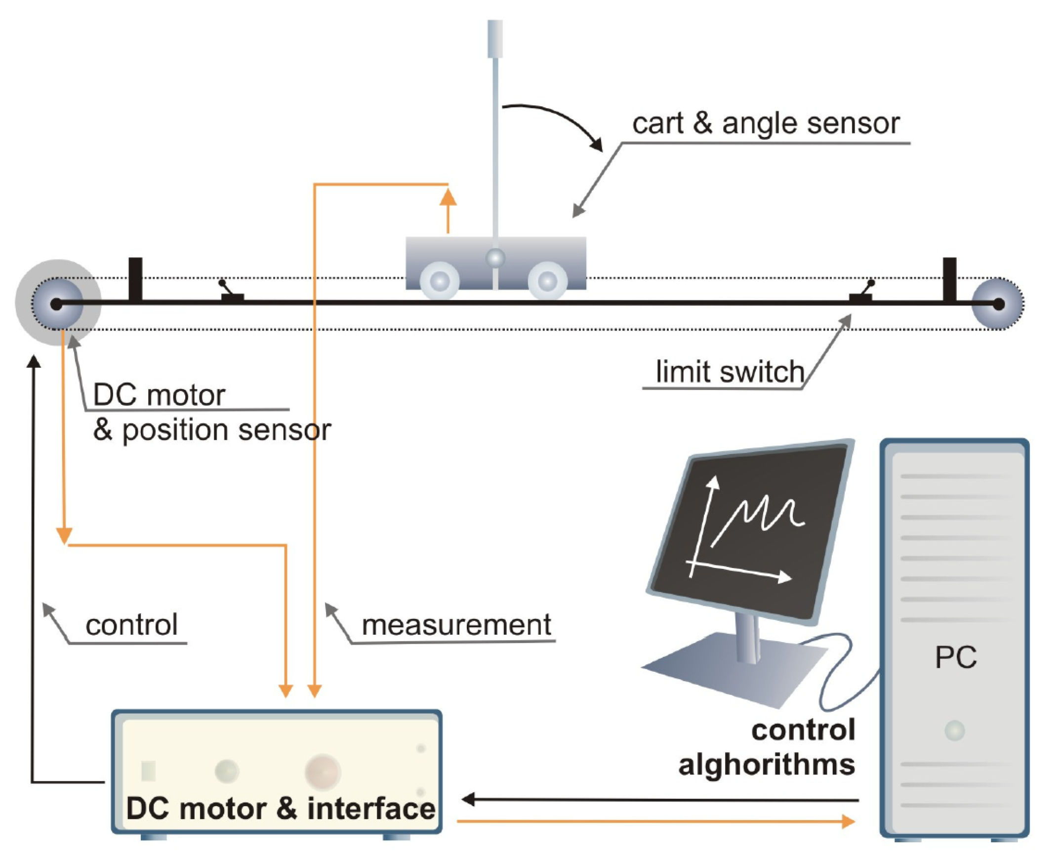
Figure 3.
Diagram of the mechanical unit of the InvP system [27].
Figure 3.
Diagram of the mechanical unit of the InvP system [27].

Figure 4.
Connection diagram between the mechanical unit, the DC & motor interface unit, and the computer, where the SCSI adapter and the Advantech PCI-1711U-CE data acquisition card are involved [27].
Figure 4.
Connection diagram between the mechanical unit, the DC & motor interface unit, and the computer, where the SCSI adapter and the Advantech PCI-1711U-CE data acquisition card are involved [27].
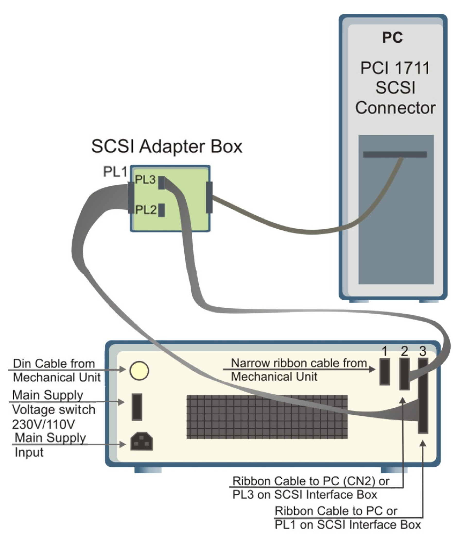
Figure 5.
Representative block diagram of PInv system for simulation purposes, programmed in Matlab/Simulink.
Figure 5.
Representative block diagram of PInv system for simulation purposes, programmed in Matlab/Simulink.
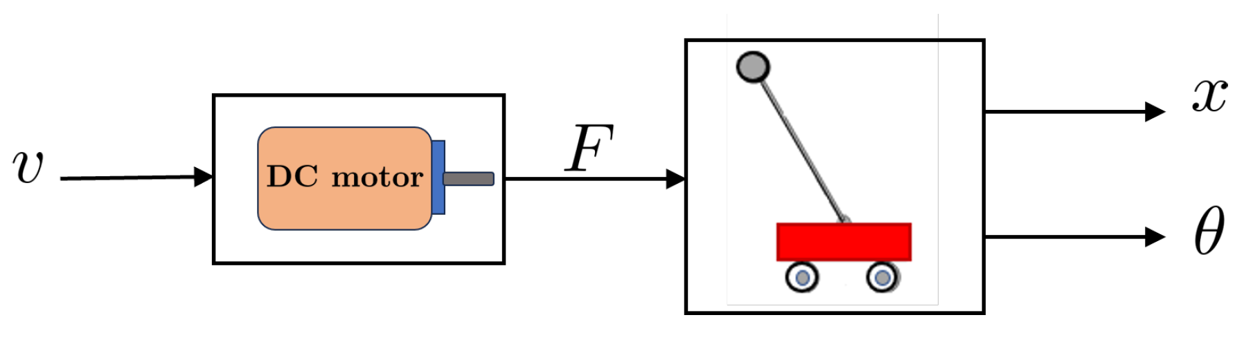
Figure 6.
Block diagram for stabilization control of the InvP using PID controllers, proposed by the manufacturer.
Figure 6.
Block diagram for stabilization control of the InvP using PID controllers, proposed by the manufacturer.

Figure 7.
Block diagram for stabilization control of the InvP using the proposed switched approach.
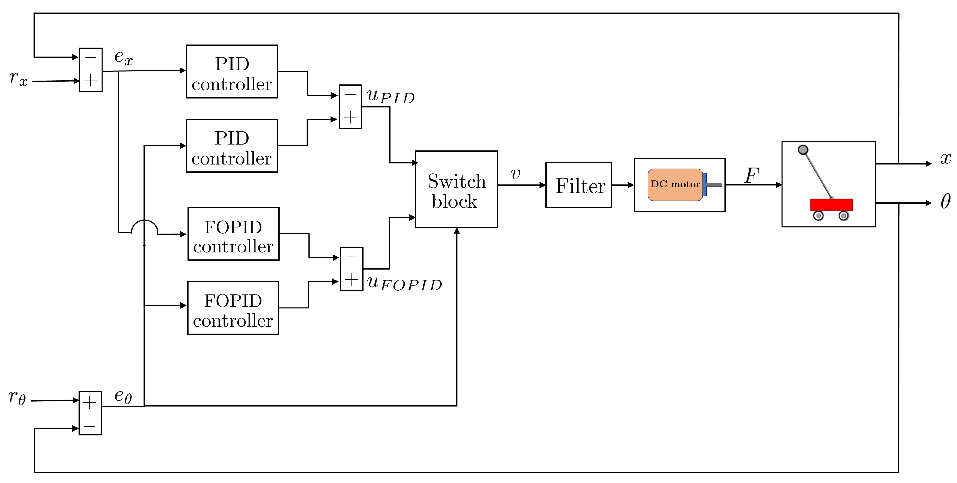
Figure 8.
Block Feedback Encoder present in the manufacture software for InvP system, to be used with Matlab/Simulink.
Figure 8.
Block Feedback Encoder present in the manufacture software for InvP system, to be used with Matlab/Simulink.
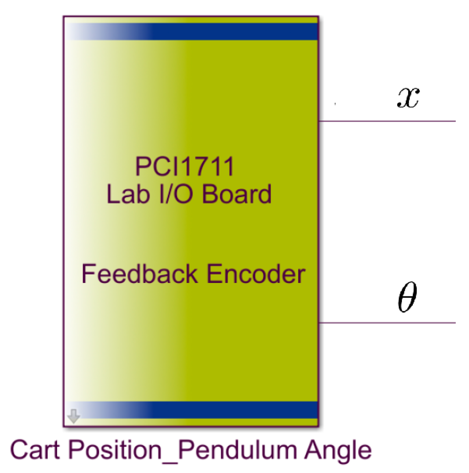
Figure 9.
Block Feedback DAC present in the manufacture software for InvP system, to be used with Matlab/Simulink.
Figure 9.
Block Feedback DAC present in the manufacture software for InvP system, to be used with Matlab/Simulink.
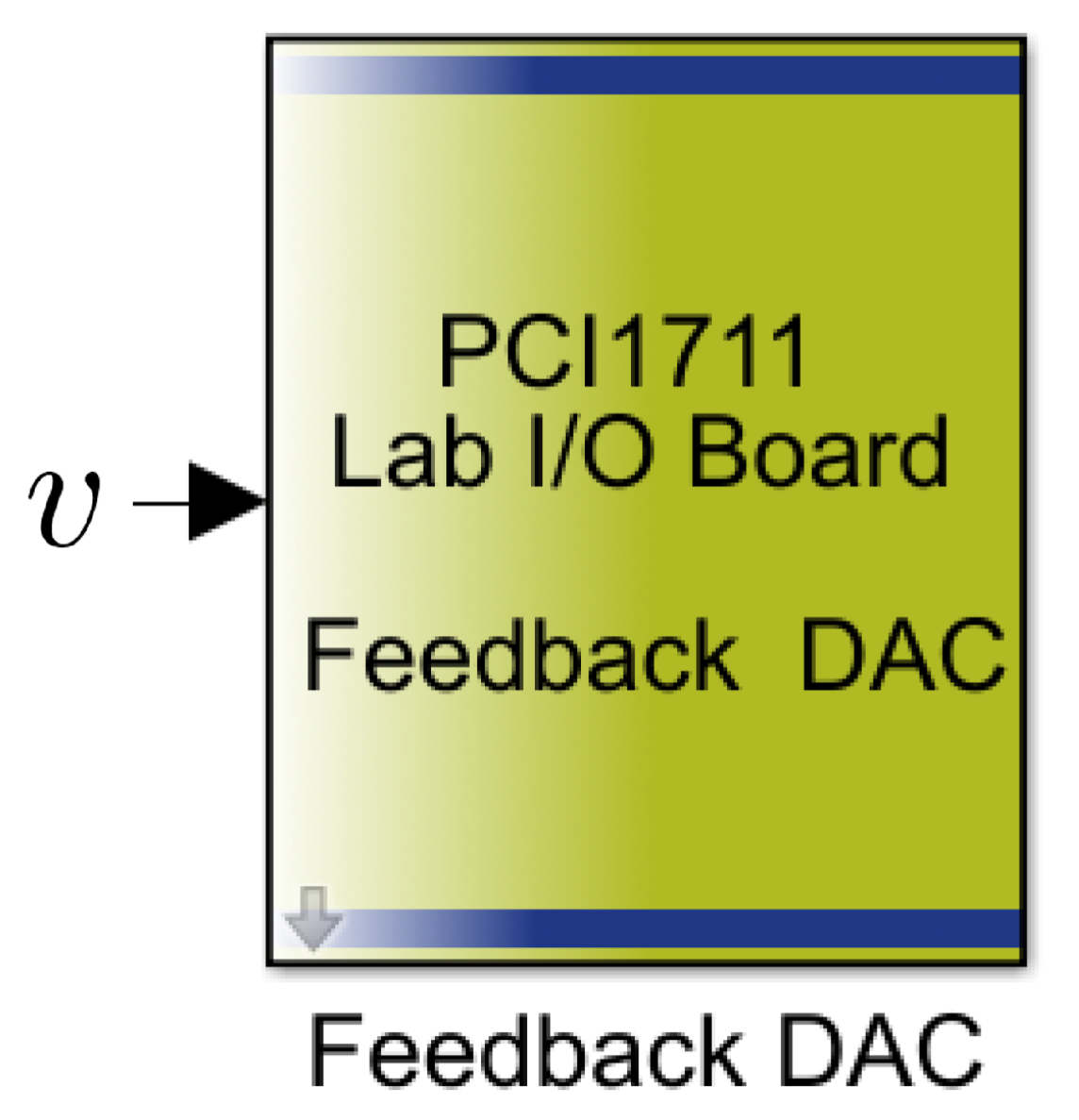
Figure 10.
Block diagram in Matlab/Simulink for experiment Swing hold pendulum extra[27].
Figure 10.
Block diagram in Matlab/Simulink for experiment Swing hold pendulum extra[27].
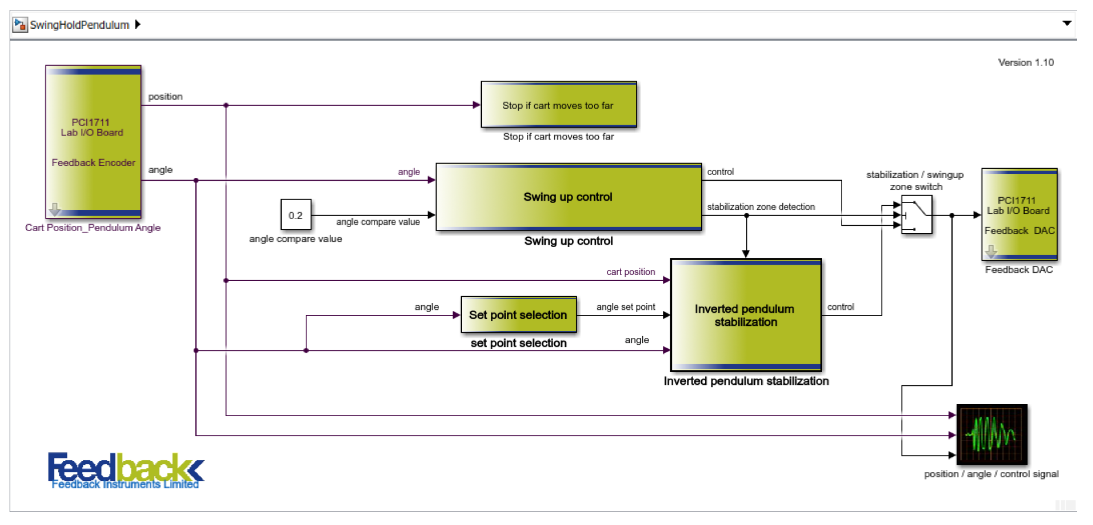
Figure 11.
Evolution of the cart position, pendulum angular position, and control signal in experimental tests, using the and the proposed PID, FOPID, and SW FOPI-PID controllers.
Figure 11.
Evolution of the cart position, pendulum angular position, and control signal in experimental tests, using the and the proposed PID, FOPID, and SW FOPI-PID controllers.
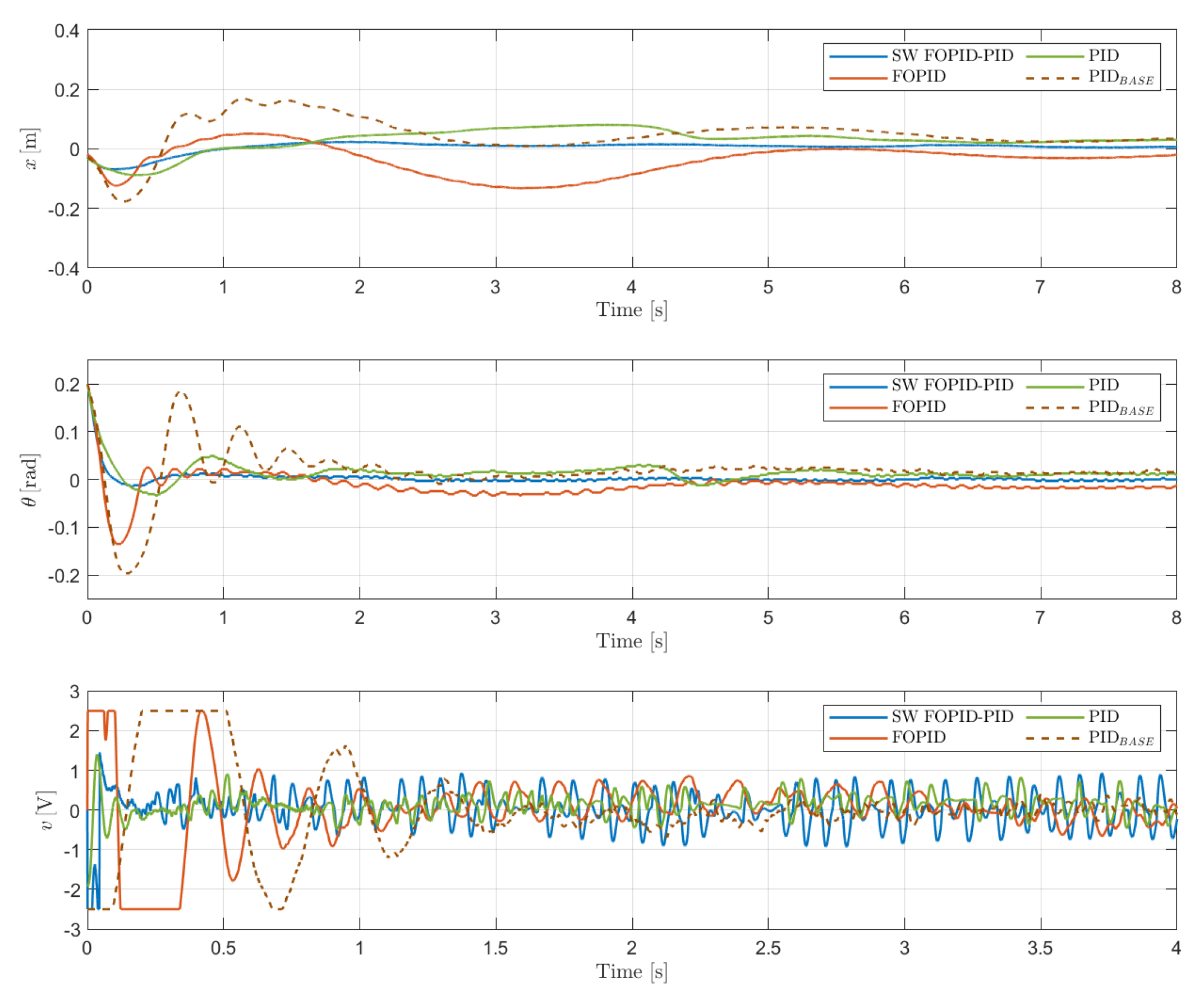
Figure 12.
Evolution of the ITAE performance indicator in experimental tests, using the and the proposed PID, FOPID, and SW FOPI-PID controllers.
Figure 12.
Evolution of the ITAE performance indicator in experimental tests, using the and the proposed PID, FOPID, and SW FOPI-PID controllers.
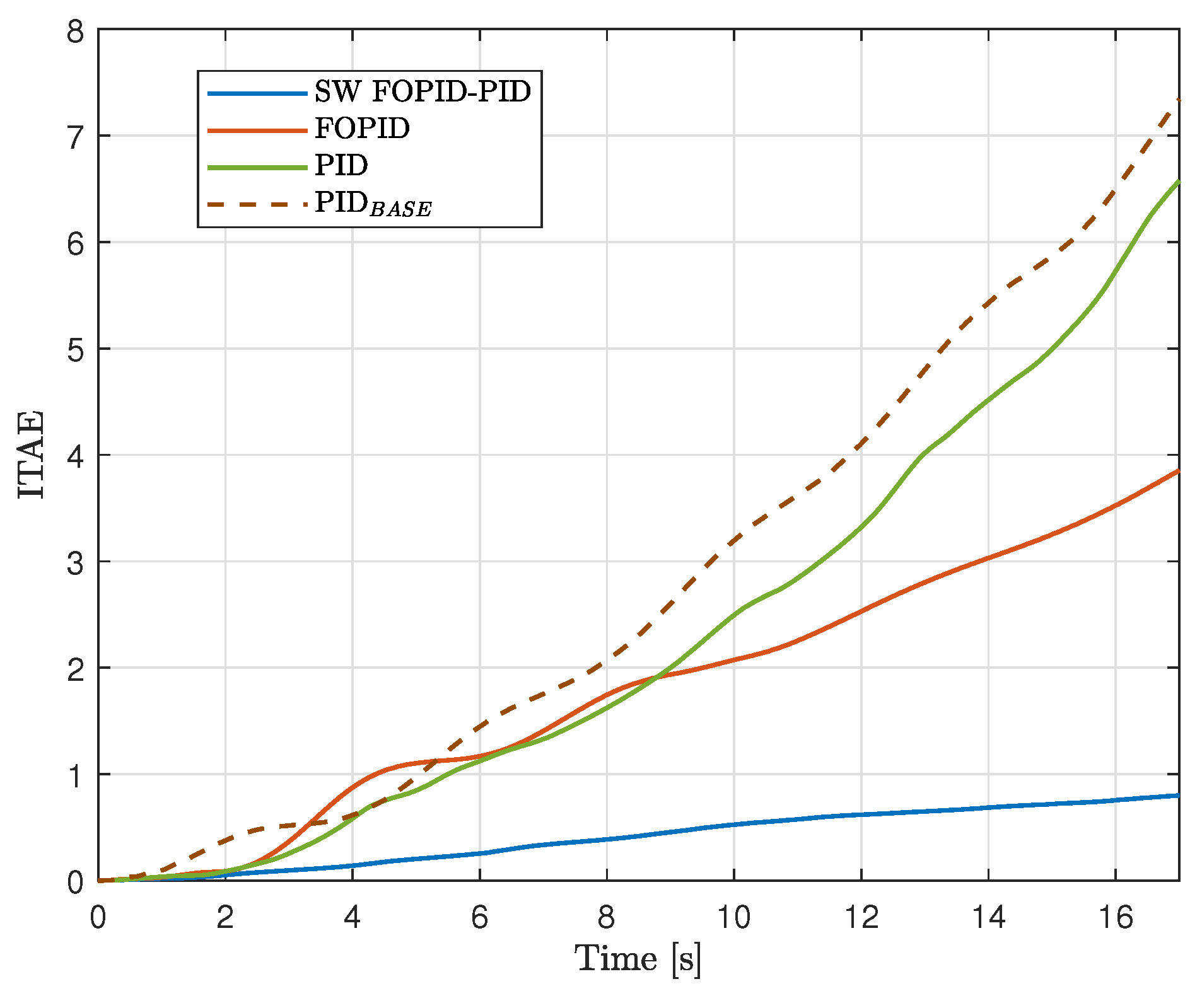
Figure 13.
Evolution of the ISI performance indicator in experimental tests, using the and the proposed PID, FOPID, and SW FOPI-PID controllers.
Figure 13.
Evolution of the ISI performance indicator in experimental tests, using the and the proposed PID, FOPID, and SW FOPI-PID controllers.
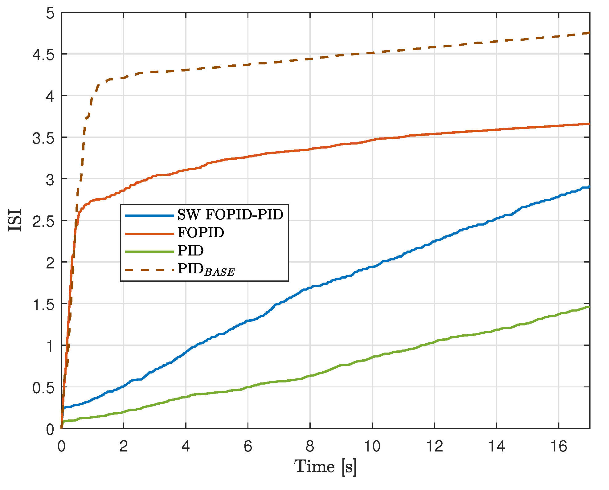
Figure 14.
Evolution of the cart position, pendulum angular position, and control signal in experimental tests, using the and the proposed PID, FOPID, and SW FOPI-PID controllers, in the presence of external disturbances.
Figure 14.
Evolution of the cart position, pendulum angular position, and control signal in experimental tests, using the and the proposed PID, FOPID, and SW FOPI-PID controllers, in the presence of external disturbances.
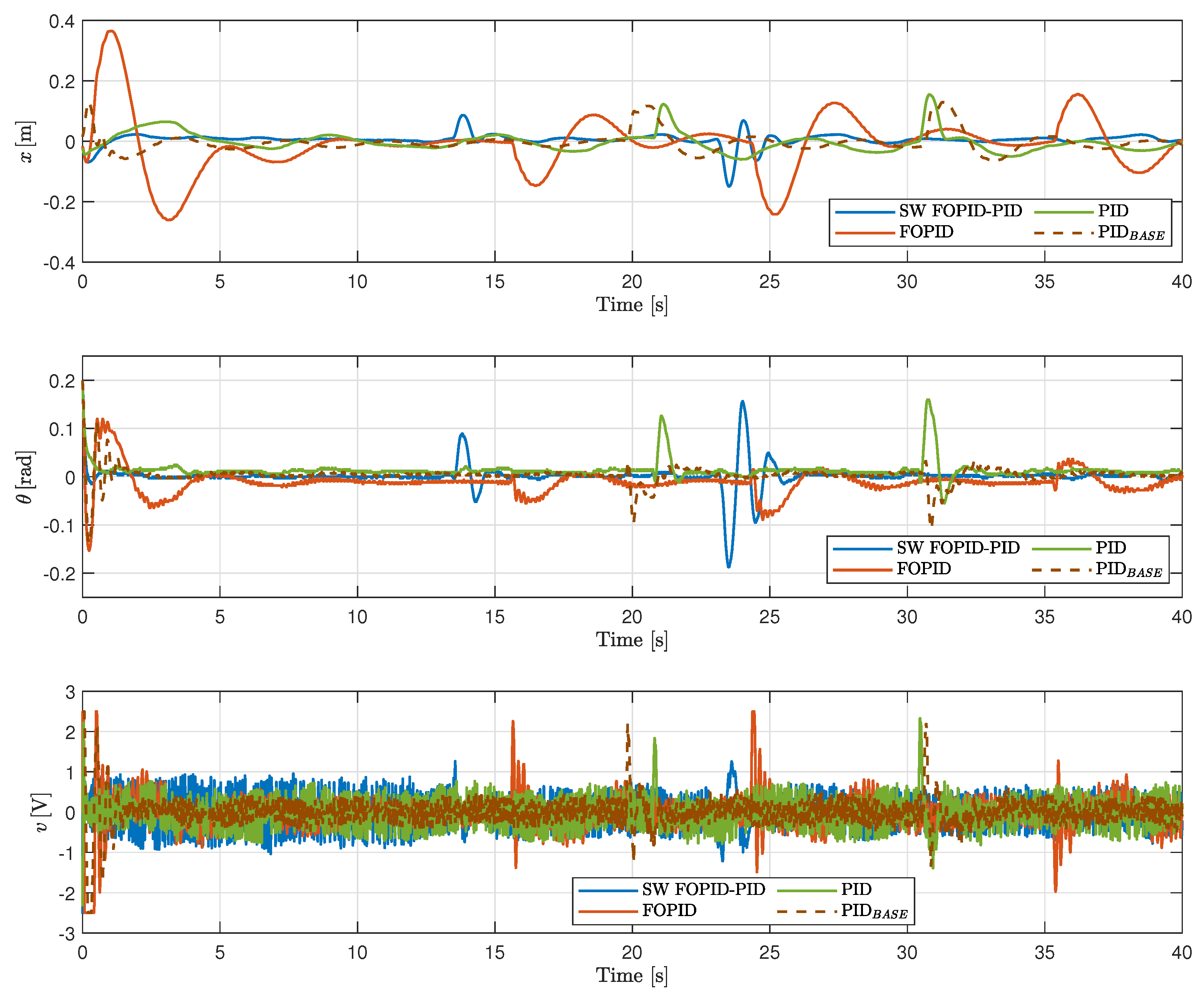
Figure 15.
Evolution of the ITAE performance indicator for controllers in an experimental test in the presence of external disturbances.
Figure 15.
Evolution of the ITAE performance indicator for controllers in an experimental test in the presence of external disturbances.
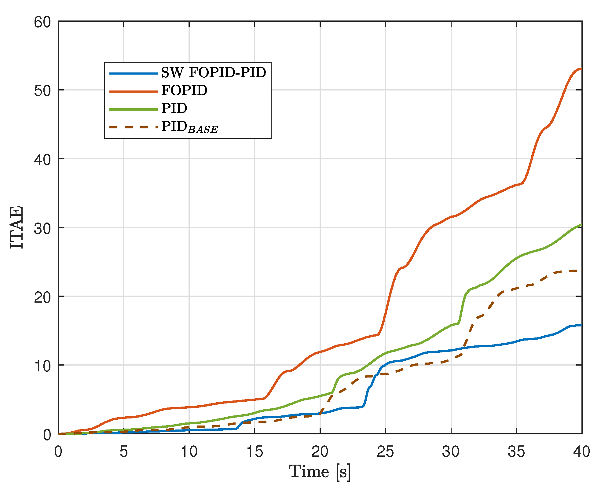
Figure 16.
Evolution of the ISI performance indicator for controllers in an experimental test in the presence of external disturbances.
Figure 16.
Evolution of the ISI performance indicator for controllers in an experimental test in the presence of external disturbances.
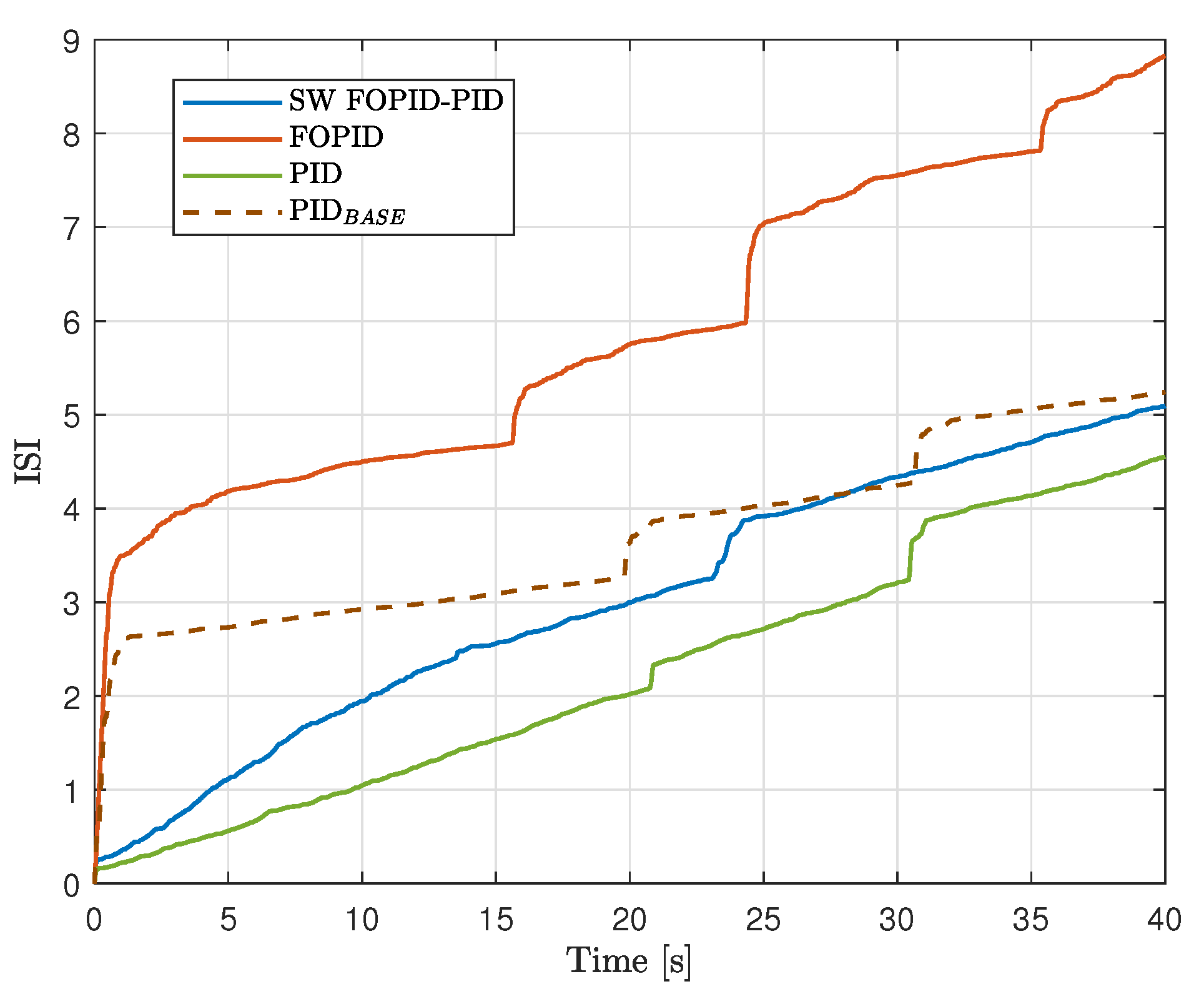

Table 1.
Numerical values of the model parameters for the InvP system (cart-pendulum and DC motor) [27].
Table 1.
Numerical values of the model parameters for the InvP system (cart-pendulum and DC motor) [27].
| Parameter | Value | Unit | Description |
|---|---|---|---|
| Cart-Pendulum system | |||
| g | 9.81 | [m/s2] | Gravitational acceleration |
| l | 0.36 | [m] | Pendulum length |
| M | 2.4 | [kg] | Mass of the cart |
| m | 0.23 | [kg] | Mass of the pendulum |
| I | 0.099 | [kg m2] | Moment of inertia |
| b | 0.05 | [N/rad/s] | Friction coefficient of the cart |
| d | 0.005 | [Nms/rad] | Viscous friction coefficient of the pendulum |
| DC Motor | |||
| 0.05 | [Nm/A] | Torque constant | |
| 0.05 | [Vs/rad] | Electromotive constant | |
| R | 2.5 | [] | Electrical resistance |
| L | 0.0025 | [H] | Electrical inductance |
| J | 0.000014 | [/rad] | Rotor’s moment of inertia |
| B | 0.000001 | [Nms/rad] | Friction coefficient |
Table 2.
Numerical values of the parameters for controller provided by manufacturer [27].
Table 2.
Numerical values of the parameters for controller provided by manufacturer [27].
| 7 | 0.5 | 4 | 25 | 0.2 | 1.5 |
Table 3.
Resulting parameters from the optimization process for all designed controllers.
| SW-FOPID-PID controller | ||||||
| 8.85 | 0.86 | 6.82 | - | - | 0.12 | |
| 19.11 | 5.25 | 3.61 | - | - | ||
| -2.25 | 2.43 | 0.88 | 0.91 | 0.40 | ||
| 33.41 | 0.78 | -2.17 | 1.56 | 0.56 | ||
| PID controller | ||||||
| 4.53 | 0.58 | 4.82 | - | - | - | |
| 8.95 | 1.61 | 2.44 | - | - | - | |
| FOPID controller | ||||||
| 2.02 | 3.32 | 11.13 | 0.86 | 0.56 | - | |
| 48.36 | -0.03 | 6.27 | 1.08 | 0.69 | - | |
Table 4.
Results obtained for the performance indicators in experimental tests to stabilize the InvP system using the designed controllers.
Table 4.
Results obtained for the performance indicators in experimental tests to stabilize the InvP system using the designed controllers.
| PID | 4.75 | 7.34 | 0.18 | 0.19 | 5.99 | 17 | 2.79e-01 | 1.90e-03 | 1.10e-03 |
| SW FOPID-PID | 2.91 | 0.20 | 0.07 | 0.015 | 0.45 | 0.94 | 1.71e-01 | 1.71e-04 | 1.09e-04 |
| FOPID | 3.66 | 3.85 | 0.13 | 0.13 | 4.38 | 17 | 2.15e-01 | 1.50e-03 | 3.35e-04 |
| PID | 1.46 | 6.57 | 0.09 | 0.05 | 4.35 | 16.8 | 8.53e-02 | 7.26e-04 | 1.82e-04 |
Table 5.
Results obtained for the performance indicators in experimental tests to stabilize the InvP system using the designed controllers, in the presence of disturbances.
Table 5.
Results obtained for the performance indicators in experimental tests to stabilize the InvP system using the designed controllers, in the presence of disturbances.
| 5.24 | 23.85 | 0.13 | 0.14 | 33.58 | 36.86 | 0.13 | 1.1e-03 | 3.3e-04 | |
| SW FOPID-PID | 5.09 | 15.81 | 0.14 | 0.18 | 24.64 | 25.62 | 0.12 | 4.16e-04 | 5.8e-04 |
| FOPID | 8.82 | 53.05 | 0.36 | 0.15 | 39.31 | 39.46 | 0.22 | 9.0e-03 | 6.9e-04 |
| PID | 4.54 | 30.43 | 0.15 | 0.16 | 33.76 | 40 | 0.11 | 1.0e-03 | 3.4e-04 |
Disclaimer/Publisher’s Note: The statements, opinions and data contained in all publications are solely those of the individual author(s) and contributor(s) and not of MDPI and/or the editor(s). MDPI and/or the editor(s) disclaim responsibility for any injury to people or property resulting from any ideas, methods, instructions or products referred to in the content. |
© 2025 by the authors. Licensee MDPI, Basel, Switzerland. This article is an open access article distributed under the terms and conditions of the Creative Commons Attribution (CC BY) license (http://creativecommons.org/licenses/by/4.0/).
Copyright: This open access article is published under a Creative Commons CC BY 4.0 license, which permit the free download, distribution, and reuse, provided that the author and preprint are cited in any reuse.


