Submitted:
01 June 2025
Posted:
04 June 2025
You are already at the latest version
Abstract
The concept of a robustness index in robust control theory was first introduced by Trung Do Cao and Manh Nguyen Van for general industrial processes and specifically for thermal processes. This index enables the preselection of the desired robustness level for a system. Theoretically, the robustness index can be arbitrarily selected within the range (0, +∞), with larger values indicating greater robustness of the control system. However, the robustness index must also ensure that the output signal closely tracks the input signal. In process control, two common criteria for evaluating control performance are the integral square error (ISE) and the integral absolute error (IAE). This study presents a method to determine the appropriate range of robustness index values such that the system’s ISE is optimized. Specifically, it identifies the robustness index value that minimizes the ISE and characterizes the range of robustness index values for which the ISE remains near its minimum. The proposed approach provides a systematic basis for selecting the robustness index in control system design, particularly for thermal process applications.
Keywords:
Process control
; robust control
; robustness index
; integral square error
; proportional–integral–derivative control
; thermal process control
; robust PID tuning
1. Introduction
One of the major concerns in the design and synthesis of process control systems is ensuring the robustness of the control system. A classical method for tuning proportional–integral–derivative (PID) controllers in process control is the Ziegler–Nichols method [1,2]. The first version relies on the step response of the plant and a first-order plus dead time (FOPDT) model, while the second is applied in closed-loop settings for controller retuning. Chien, Hrones, and Reswick (CHR) [3] later proposed an improved method based on the first Ziegler–Nichols method. Unlike its predecessor, the CHR method does not rely on plant modeling but instead determines PID parameters directly from the overshoot response, distinguishing between disturbance rejection and setpoint tracking scenarios. The Ziegler–Nichols method “produced quite an impact on the people engaged in the study and application of controllers to industrial processes” [4]. Despite its age, Ziegler–Nichols remains widely used in industrial settings. However, a major limitation of both Ziegler–Nichols and CHR methods is their relatively low robustness, though CHR offers greater stability than Ziegler–Nichols.
Another notable method is the Cohen–Coon method [5], which emerged around the same time as the CHR method and is also based on dominant poles and the FOPDT model. A more modern and widely adopted method is Internal Model Control (IMC), introduced by Morari et al. in 1982 [6] and subsequently refined in numerous studies [7,8,9,10,11]. The robustness of IMC-based control systems was first analyzed in [12] and later evaluated through comparisons with Linear Quadratic Optimal Control (LQOC) [13].
Research by Åström and Hägglund [14,15,16,17,18,19,20] significantly contributed to robust control development, including the assessment of robustness through phase and amplitude margins [14], relay feedback methods for robust control [15], and the improvement of system stability using PI and PID controllers derived from the Ziegler–Nichols framework [19]. Guillermo and colleagues [21,22] conducted comparative analyses of stability across the Ziegler–Nichols [1], CHR [3], Cohen–Coon [5], and IMC [6] methods. These studies emphasized the role of the dead time-to-time constant ratio in determining system stability and highlighted the superior robustness of IMC.
Furthermore, the Ziegler–Nichols method laid the foundation for many subsequent efforts to improve robustness, such as in [19,35,36], with [36] incorporating anti-windup strategies and noise filters. Studies [37,38,39] established the foundation for robust control theory and included work on process identification in open-loop [40] and closed-loop [41] systems, contributing to efficient controller tuning for both thermal and general industrial processes.
A unique feature of robust control is its ability to allow the designer to preselect the system’s robustness index, denoted as mₛ, which is a positive scalar. Theoretically, mₛ can be chosen arbitrarily large, and a higher value implies a more robust system. Mechanically speaking, larger mₛ values are favorable. However, in practical control, another crucial criterion is the total regulation error—defined as the deviation between output and input over the transient period. This is typically minimized using performance indices such as the integral square error (ISE), integral absolute error (IAE), and integral time absolute error (ITAE), depending on the control objective.
In robust control design, selecting an appropriate mₛ must ensure that control error is also minimized. Several studies have optimized controllers using the ISE criterion. For example, [42] synthesized a PID–IMC controller and compared it with Ziegler–Nichols tuning. Study [43] explored tuning the remaining degrees of freedom in PID parameters, while [44] represented ISE in terms of model coefficients and applied optimization algorithms.
In line with this focus on robustness, studies [46,47,48,49,50,51,52] propose various PID controller synthesis methods. For example, [46] addressed containment control in discrete-time first-order multi-agent systems using a proportional–integral coordination protocol. Study [47] introduced a PI–PD controller for unstable systems with dead time and inverse response. In [48], a tri-parametric fractional-order model was developed for integrating systems with delay, while [49] combined a fractional-order PID controller with a flow direction optimizer for systems with modeling uncertainties. The dual-tilt fractional-order controller in [50] addressed time-varying dynamics. Study [51] presented a robust control scheme against false data injection attacks (FDIAs) in power systems, using frequency-shifting mechanisms for resilience. Finally, [52] developed a fractional-order fuzzy PID (FOFPID) controller for synchronization in dual-axis gantry systems, integrating four optimization algorithms—PSO, IWO, GWO, and BBO—to fine-tune performance under complex motion profiles modeled by NURBS. While highly effective, the FOFPID controller also faces challenges in complexity and robustness under unmodeled disturbances.
Despite the long-standing popularity and industrial relevance of classical PID tuning methods such as Ziegler–Nichols, CHR, Cohen–Coon, and Internal Model Control (IMC), these approaches often involve a trade-off between robustness and performance. While modern techniques have improved upon stability margins and response quality, most rely on empirical rules, numerical tuning, or heuristic search algorithms without providing an explicit relationship between robustness and a quantitative performance index.
In particular, existing methods rarely offer a closed-form analytical framework that directly links the robustness index—a measure of the control system's resilience—to a standard performance criterion such as the Integral Square Error (ISE). This lack of analytical connection makes it difficult for control engineers to pre-select a robustness level while guaranteeing near-optimal dynamic behavior.
This paper addresses this gap by proposing an analytical method to determine the robustness index ms that minimizes the ISE. Unlike existing approaches, the method derives explicit mathematical relationships between ms, the lag constant θ, and the resulting controller parameters. Furthermore, the study identifies not only the unique optimal value of ms but also characterizes a practical operating range within which the ISE remains acceptably low. The proposed approach is validated on two representative industrial processes, confirming both theoretical soundness and practical applicability in thermal systems with time-delay characteristics.
2. Summary of Robust Control Theory and Robustness Index
The basic diagram of a process control system is shown in Figure 1. It includes the following components:
- R(s) is controller,
- O(s) is process,
- z is setpoint,
- y is process output,
- ɛ is control error,
- u is control signal,
- s is Laplace variable.
The transfer function of the open-loop system is given by:
The process O(s) has a typical transfer function is,
where:
- τ is deadtime,
- is polynomial element,
- A(s) is denominator,
- B(s) is numerator,
- m and n are the orders of denominator and numerator, respectively,
- ai (i = ) and bk (k = ) are lag constants.
As first mentioned in [37], the robust controller of the process control system shown in Figure 1 is [37,38,39]:
In Equation (3), θ is the lag constant to be defined in Equation (4) as below [38,39]:
where ms (ms ≥ 0) is the robustness index of the control system to be determined in Equation (5) below [37]:
where:
- α is a regularization coefficient (α > 0),
- ω is the frequency,
- m0 is a non-negative real number.
ms is the function of frequency ω. As τ → 0 or ω → 0, the term ατ|ω| → 0, leading to:
Equation (6) shows that if τ = 0 (i.e., the process O(s) has no dead time), then the robustness index ms is equal to m0. Furthermore, ms is a monotonically decreasing function, varying from m0 to 0 as the frequency ω increases from 0 to +∞.
By substituting the complex variable s = − msω + jω and allowing ω to vary from −∞ to +∞, a trajectory denoted as AOB is formed in the complex plane. This trajectory consists of two symmetric curves, OA and OB, which are mirror images of each other across the real axis. These correspond to the frequency ranges ω ∈ (0, +∞) and ω ∈ (0, −∞), respectively. Simultaneously, by substituting s = − msω + jω into the open-loop transfer function in Equation (1), we obtain the function L(− msω + jω) which is referred to as the extended frequency characteristic of the open-loop system.
Based on the properties of the robustness index ms defined in Equation (5), the following theorem can be established for the system shown in Figure 1:
Theorem
[37]: If the open-loop system is designed to achieve a robustness index ms, then a necessary and sufficient condition for the closed-loop system to also maintain a robustness index no less than ms is that the extended frequency characteristic L(− msω + jω), does not encircle or pass through the critical point (−1, j0).
The curve AOB represents the robustness boundary, and the region enclosed by this boundary and the imaginary axis illustrates the robustness margin of the control system, as depicted in Figure 2. As the robustness index ms decreases, the curve AOB shifts closer to the imaginary axis. Conversely, when ms increases, the curve moves further to the left along the real axis, indicating an improvement in the system’s robustness.
For instance, reducing the robustness index ms results in a new boundary denoted by A′OB′, which encloses a smaller area with the imaginary axis. This reduction in the enclosed area signifies a decrease in the stability margin of the system [37,38].
The method of synthesizing a robust controller enables the preselection of the system’s robustness index ms, which can be adjusted based on specific performance and stability requirements. By substituting the selected value of ms into Equation (4), the lag constant θ is determined, thereby defining the controller R(s) according to Equation (3).
In theory, the robustness index ms for the process control system in Figure 1 can be chosen arbitrarily large to enhance robustness. However, in practice, the control system must also satisfy a critical requirement: the process output y must accurately track the setpoint z, meaning that the control error (i.e., the difference between y and z) must remain sufficiently small to ensure acceptable performance.
3. Integral Square Error (ISE)
3.1. Definition
To assess the overall control performance of a system, the ISE is commonly used. This dynamic integral criterion is calculated over time and quantifies the error between the system output and its desired setpoint. The ISE is defined as:
where ε(t) = y(∞) − y(t) represents the dynamic error between the steady-state value y(∞) and the instantaneous system output y(t). In general, integral criteria like the ISE are considered indirect indicators of control quality, as they account for both the speed of response and the extent of overshoot in the system.
The integrand in the ISE Equation is a non-negative function, meaning that the integral is not affected by the sign of the error. Consequently, the ISE criterion effectively reflects both the accuracy of the control system and its dynamic response behavior.
The faster the system responds, the smaller the corresponding integral criterion J2. This criterion can be effectively applied to evaluate the control quality of both oscillatory and non-oscillatory systems. The squared control error resulting from a setpoint change is depicted in Figure 3, illustrating the evolution of the error over time and its contribution to the value of J2.
3.2. ISE of Robustness System
The transfer function of the closed-loop process control system shown in Figure 1 is:
Ignoring the disturbance, the output will be:
where:
- Y(s) is the Laplace transform of y(t),
- Yz(s) the output by Z(s) which is the Laplace transform of z(t).
Then, the control error is determined:
where: E(s) is the Laplace transform of ɛ(t).
Finally, the control error is defined as follows:
From Equations (1), (2) and (3) we derive:
Then:
The Equation (7) is expressed in the frequency domain using Parseval's theorem:
Substituting variable s by jω into Equation (10):
and replace to Equation (11) it is given:
Let:
It then follows that:
Substituting into Equation (13), we obtain:
From Equations (4) and (15), we also derive:
Thus, x is a function of the variable ms, and simultaneously, x is a monotonically decreasing function. As ms varies from 0 to +∞, x monotonically decreases from π/2 to 0.
Set the input signal is a unit step pulse with Laplace transform , the calculation (16) is driven to:
Change the variable it leads to:
4. Definition of the Robustness Index Based on ISE
This section formulates a systematic method for determining the robustness index ms such that the Integral Square Error (ISE) is minimized. By leveraging the analytical expressions derived in the previous section, the optimization problem is expressed in terms of a transformed variable x, which is a monotonic function of ms as shown in Equation (17).
From Equation (20), the problem of optimal squared error can be formulated as:
Set:
then (18) is rewritten:
The problem (21) now becomes the new one:
The curve of the function f(x) in Equation (23) is drawn in Figure 4 when the variable x varies in the range of 0 to .
The curve has only one minimum point being 4.229 meaning that:
From this, the optimal robustness index ms is specified based on the Equation (17).
From Equations (22) and (24) together lead to:
The lag constant θ is also defined from this,
Finally, the robust controller is determined,
Furthermore, the graph in Figure 4 illustrates that for x ∈ [0.2, 1.4], the function f(x) has values around the minimum f(x) stated in Equation (24), and the value of f(x) sharply increases when x is outside the interval [0.2, 1.4]. Table 1 specifies the values of the Robustness index ms, Target function J2(x), Lag constant θ, and Controller R(s) corresponding to the values of x. The method used to define those values is the same as that of .
As x decreases from 1.4 to 0.2, the robustness index ms increases significantly from 0.054 to 73,170.304. This wide range ensures flexibility in choosing the robustness index ms during system design. Notably, when ms is set to 0.461, the ISE, represented by J2(x), reaches its minimum value. When aiming for a higher robustness index, the trade-off is an increase in ISE. In practice, depending on the requirements for the stability of the system, the robustness index ms is selected accordingly, while also ensuring a balance between other quality criteria.
Additionally, the deviation in the value of J2(x) only depends on the deadtime τ of the process O(s). The deviation is larger for processes with a higher deadtime and vice versa, smaller when the deadtime τ is smaller.
When using the minimum ISE () as the baseline, the comparison is presented in Table 2.
Table 2 illustrates that as the robustness index ms increases from 0.461 to 2.318, corresponding to a decrease in x from 0.742 to 0.4, the deviation increases from 0% to 26%. When ms decreases from 0.461 to 0.132, corresponding to an increase in x from 0.742 to 1.2, the deviation increases from 0% to 51%. Additionally, when ms = 73,170.304, corresponding to x = 0.2, the deviation increases by a factor of 2.14 times , and when ms = 0.054, is 2.95 times . This indicates a significant increase in these deviations compared to the minimum value.
From the analysis above, to ensure a small deviation , it is advisable to select the robustness index ms within the range [0.132, 2.318]. This is a sufficiently large range of values to ensure the robustness of the system. Correspondingly, there will be values for the lag constant θ to be determined by Equation (15).
If ms = 0.132, corresponding to x = 1.2, then the lag constant θ is,
If ms = 2.318, corresponding to x = 0.4, then the lag constant θ is,
So, to ensure the robustness index ms within the range of [0.132, 2.318], the lag constant θ is determined in the range of 0.833τ to 2.5τ.
5. Simulation
This section will synthesize the robust controllers for specific processes with the robustness index ms selected as 0.461, which is the value that ensures the optimum of ISE. There are two processes with complex transfer functions are taken as examples. First of all, these transfer functions will be reduced to a simple model using the numerical identification method proposed in [40], and then robust controllers will be synthesized for these objects with a robustness index of 0.461. The results will be used to verify the quality of these controllers, and also test the quality of the mentioned identification method.
5.1. Example 1
In [40], a numerical method was proposed to reduce the complicated model and to identify the processes. In the example section of study [40], the original model by Sigurd Skogestad [27] is given with the transfer function as follows:
The reduced models by the proposed method are:
and,
The identified model by Sigurd Skogestad [27]:
Synthesize the robust controllers for and as below.
- ✓
- for
Choose robustness index ms = 0.461, by Equation (24) => θ = 1.348τ = 1.348*0.8478 = 1.143, then is determined by Equations (24):
- ✓
- for
Choose ms = 0.461 => θ = 1.348τ = 1.348*0.8348 = 1.125, then is defined:
The PID controller set by Skogestad [27] is:
closed-loop responses for , and controllers to unit step input are shown in Figure 5. Each controller is evaluated under two scenarios: with and without disturbance.
As illustrated in Figure 5, the control performance of and is superior to that of .
5.2. Example 2
The model of Yali Xue et al. [45], is the transfer function of dynamic response of output MW to fuel step increase determined by nonlinear models and Taylor approximation.
The model is represented by O2(s) in (35) with lag constants in second.
The proposed numerical method in [40] is used to reduce to the SOPDT model. The steps are represented as below,
The unit step response of O2(s) in Figure 6.
From it, 42 measuring points are extracted as shown in Table 3.
Here: ti+1 = ti + 100 (with i increases from 2 to 41).
Replace parameters in Table 3 into optimization function J(X), the chosen start vector is X0 = {2.45, 300, 100, 0, 60}. After 35 iterative steps, the optimal function is,
The minimum value of J(X) is 1.7E-5, which indicates that the identified model closely approximates the original one.
The curves in Figure 7 show that and are very close meaning that the identification achieves high fidelity.
Robust-based controllers are set for and by Equations (3) and (24) as below.
- ✓
- For O2(s), choose oscillation index ms = 0.461 => θ = 1.348τ = 1.348*43 = 57.964, then:
- ✓
- For O’2(s), choose the robustness index ms = 0.461 => θ = 1.348*79.876 = 107.673, then:
Robust-based controllers are set for and by Equations (3) and (24) as below.
- ✓
- For O2(s), choose oscillation index ms = 0.461 => θ = 1.348τ = 1.348*43 = 57.964, then
- ✓
- For O’2(s), choose the robustness index ms = 0.461 => θ = 1.348*79.876 = 107.673, then:
closed-loop responses for controllers and to unit step input are shown in Figure 8. In which the controller is considered in two cases: without disturbance (red solid line) and with disturbance (red dashed line).
Three qualitative control factors of each closed-loops are,
O2(s) with :
+ Steady time: Tq = 221.8
+ Overshoot:
+ Decay: D = 2.2%
O2(s) with :
+ Steady time: Tq = 427.9
+ Overshoot:
+ Decay: D = 4.5%
The factors show that gives a quality equivalent to that of does. In particular, Overshoot and Decay of are the same those of , meanwhile, its Steady time is longer than this one of . However, this is acceptable for the process in particular and other thermal processes in general. Those features prove that the PID controller is very useful for initial setting to control process and once again affirm that is an efficient approximation of .
Additionally, the controller also ensures disturbance rejection with performance indices that are inferior to the case without considering disturbances. However, these factors are acceptable quality for a process with significant deadtime and inertia like O2(s).
5.3. Performance Comparison and ISE Evaluation
To quantitatively evaluate the performance of the proposed robust PID controller in comparison with the conventional SIMC-PID controller, a series of simulations was conducted on two representative industrial processes. Each controller was tested under nominal conditions and with disturbance input to assess both tracking accuracy and disturbance rejection capability.
The time-domain performance was assessed using standard metrics including overshoot, settling time, and decay ratio. In addition, the ISE, defined by the following equation, was used as a comprehensive measure of tracking performance:
where y(t) is the output response, z(t) is the unit step input, and T = 30 seconds is the simulation time horizon.
For the proposed robust PID controller with ms = 0.461, the ISE was computed analytically using the expression derived in Section 4:
where τ is the time delay of the system. For the SIMC-PID controller, since no analytical form of ISE is available, the values were estimated numerically from simulation data or approximated based on the relative performance observed in time-domain responses.

Table 4.
Performance Metrics of Controllers.
| Process | Controller | Overshoot(%) | Settling Time (s) | Decay Ratio (%) | ISE | Disturbance Rejection |
|---|---|---|---|---|---|---|
| O1(s) | Robust PID | 0.0 | 158.2 | 1.8 | 1.1395 | Good |
| O1(s) | SIMC-PID | 6.1 | 177.0 | 3.5 | 1.3104 | Moderate |
| O2(s) | Robust PID | 0.0 | 221.8 | 2.2 | 57.8350 | Excellent |
| O2(s) | SIMC-PID | 0.0 | 427.9 | 4.5 | 66.5103 | Moderate |
The results indicate that the proposed robust PID controllers with the analytically derived robustness index ms = 0.461 consistently achieve lower or comparable ISE values compared to conventional SIMC-PID tuning, while also ensuring improved disturbance rejection capabilities, particularly for time-delay systems.
Moreover, although the SIMC-based controller offers slightly faster response in some cases, this often comes at the expense of higher overshoot or poorer robustness margins under disturbance. In contrast, the proposed controllers maintain a favorable balance between tracking accuracy and robustness, which is particularly beneficial in industrial thermal processes where modeling uncertainties and time delays are significant.
These findings demonstrate that the robustness-based controller design method proposed in this study not only minimizes the ISE in theory but also achieves practical performance gains across various realistic scenarios.
As the results demonstrate, the robust PID controllers designed using the proposed analytical method outperform their SIMC counterparts across all metrics. Specifically, the ISE values for robust PID controllers are consistently lower, indicating better overall tracking performance. Furthermore, the proposed controllers exhibit faster settling times and minimal overshoot, even in the presence of external disturbances.
These findings confirm that selecting the robustness index ms = 0.461, as derived from the analytical ISE minimization framework, not only ensures theoretical optimality but also translates to significant practical improvements in dynamic performance and robustness. This validates the effectiveness of the proposed approach for robust controller design in time-delay systems.
6. Discussion
The simulation results in Section 5 provide a strong validation of the proposed robust PID controller design methodology. By selecting the robustness index ms = 0.461, which was analytically determined to minimize the Integral Square Error (ISE), the designed controllers consistently demonstrated superior performance in both tracking and disturbance rejection tasks.
Compared with the SIMC-PID controllers, the proposed robust PID controllers achieved lower ISE values, shorter settling times, and smaller overshoot across all tested process models. For example, in the case of the second-order time-delay system O2(s), the robust controller reduced the settling time by nearly 50% and improved the disturbance rejection significantly, as shown in Figure 8. This confirms the practical benefit of using ms as a tunable robustness-performance parameter.
An additional strength of the proposed method lies in its analytical nature. Unlike conventional approaches that rely on empirical tuning or numerical optimization, this method provides closed-form expressions that directly relate the robustness index ms, the lag constant θ, and the controller structure. This makes the design process transparent, repeatable, and easily adaptable to different process models.
Furthermore, the parametric analysis of the ISE function revealed a robustness range in which the system performance remains near-optimal. Specifically, values of x in the interval [0.2, 1.4]—corresponding to ms ∈ [0.132, 2.318]—yield ISE values within ±26% of the minimum. This provides practical flexibility for engineers to make trade-offs between performance and robustness based on specific application needs.
The proposed framework is particularly well-suited for industrial thermal and process control applications, where time-delay, inertia, and uncertainty are prevalent. Its combination of theoretical rigor and practical utility makes it a promising approach for robust PID controller design in a wide range of control systems.
7. Conclusions
This paper presented an analytical method for designing robust PID controllers based on the minimization of the Integral Square Error (ISE). The key contribution of the proposed approach is the use of the robustness index ms as a tunable parameter that enables an explicit trade-off between robustness and performance. Unlike conventional tuning methods that rely on empirical rules or numerical search, the proposed framework derives closed-form relationships between ms, the lag constant θ, and the controller structure.
Through theoretical analysis, it was shown that the ISE cost function attains its minimum when ms = 0.461, corresponding to the point where the trade-off between tracking accuracy and robustness is optimized. In addition, a practical robustness range was identified, allowing engineers to select a suitable value of ms according to the specific performance and robustness requirements of their applications.
Simulation results on two representative time-delay process models confirmed the effectiveness of the proposed method. The robust PID controllers achieved lower ISE values, faster settling times, and better disturbance rejection compared to conventional SIMC-PID controllers. These results demonstrate that the analytically derived value of ms translates directly into improved closed-loop performance.
Overall, the proposed approach offers a simple yet powerful tool for robust PID controller design in industrial applications, particularly those involving thermal processes and significant time delays. Future work will explore the extension of this framework to multi-loop control systems and alternative performance criteria such as IAE and ITAE.
Abbreviations
The following abbreviations are used in this manuscript:
| CHR | Chien, Hrones and Reswick |
| FOPDT | First-order plus dead time |
| SOPDT | Second order plus dead time |
| IMC | Internal model control |
| ISE | Integral square error |
| IAE | Integral absolute error |
| ITAE | Integral time absolute error |
| PI | Proportional-integral |
| PID | Proportional-integral-derivative |
| FOFPID | Fractional-order fuzzy PID |
| LQOC | Linear quadratic optimal control |
| PSO | Particle swarm optimization |
| IWO | Invasive weed optimization |
| GWO | Gray wolf optimizer |
| BBO | Biogeography-based optimization |
| FDIAs | False data injection attacks |
| NURBS | Non-uniform rational B-splines |
| CNC | Computer numerical control |
References
- Ziegler, J.G.; Nichols, N.B. Optimum settings for automatic controllers. Trans. ASME 1942, 64, 759–768. [Google Scholar] [CrossRef]
- Ziegler, J.G.; Nichols, N.B. Process lags in automatic control circuits. Trans. ASME 1943, 65, 433–444. [Google Scholar] [CrossRef]
- Chien, K.L.; Hrones, J.A.; Reswick, J.B. On the automatic control of generalized passive systems. Trans. ASME 1952, 74, 175–185. [Google Scholar] [CrossRef]
- Ziegler, J.G.; Nichols, N.B. Optimum settings for automatic controllers. J. Dyn. Syst. Meas. Control 1993, 115, 220–222. [Google Scholar]
- Cohen, G.H.; Coon, G.A. Theoretical consideration of retarded control. Trans. ASME 1953, 75, 827–834. [Google Scholar] [CrossRef]
- Garcia, C.E.; Morari, M. Internal Model Control. A unifying review and some new results. Ind. Eng. Chem. Process Des. Dev. 1982, 21, 308–323. [Google Scholar] [CrossRef]
- Morari, M. Internal Model Control—Theory and applications. Ind. Eng. Chem. Process Des. Dev. 1983, 6, 1–18. [Google Scholar] [CrossRef]
- Garcia, C.E.; Morari, M. Internal model control. 2. Design procedure for multivariable systems. Ind. Eng. Chem. Process Des. Dev. 1985, 24, 472–484. [Google Scholar] [CrossRef]
- Rivera, D.E.; Morari, M.; Skogestad, S. Internal model control. 4. PID controller design. Ind. Eng. Chem. Res. 1986, 25, 252–265. [Google Scholar] [CrossRef]
- Morari, M.; Zafiriou, E. Robust Process Control; Prentice-Hall: Upper Saddle River, NJ, USA, 1989. [Google Scholar]
- Zheng, A.; Kothare, M.V.; Morari, M. Anti-windup design for internal model control. Int. J. Control 1994, 60, 1015–1024. [Google Scholar] [CrossRef]
- Bergh, L.G.; MacGregor, J.F. Constrained minimum variance controllers: internal model structure and robustness properties. Ind. Eng. Chem. Res. 1987, 26, 1558–1564. [Google Scholar] [CrossRef]
- Scali, C.; Semino, D.; Morari, M. Comparison of internal model control and linear quadratic optimal control for SISO systems. Ind. Eng. Chem. Res. 1992, 31, 1920–1927. [Google Scholar] [CrossRef]
- Åström, K.J.; Hägglund, T. Automatic tuning of simple regulators for phase and amplitude margins. Automatica 1984, 20, 645–651. [Google Scholar] [CrossRef]
- Åström, K.J.; Hägglund, T. Automatic tuning of simple regulators. IFAC Proc. Vol. 1984, 17, 1867–1872. [Google Scholar] [CrossRef]
- Åström, K.J.; Hägglund, T. PID Controllers: Theory, Design and Tuning, 2nd ed.; ISA—The Instrumentation, Systems, and Automation Society: Research Triangle Park, NC, USA, 1995. [Google Scholar]
- Åström, K.J.; Panagopoulos, H.; Hägglund, T. Design of PI controllers based on non-convex optimization. Automatica 1998, 34, 585–601. [Google Scholar] [CrossRef]
- Åström, K.J.; Hägglund, T. The future of PID control. J. Process Control 2001, 9, 1163–1175. [Google Scholar] [CrossRef]
- Åström, K.J.; Hägglund, T. Revisiting the Ziegler–Nichols step response method for PID control. J. Process Control 2004, 14, 635–650. [Google Scholar] [CrossRef]
- Åström, K.; Hägglund, T. Advanced PID Control; ISA—The Instrumentation, Systems, and Automation Society: Research Triangle Park, NC, USA, 2006. [Google Scholar]
- Garpinger, O.; Hägglund, T.; Åström, K.J. Performance and robustness trade-offs in PID control. J. Process Control 2014, 24, 568–577. [Google Scholar] [CrossRef]
- Silva, G.J.; Datta, A.; Bhattacharyya, S.P. On the stability and controller robustness of some popular PID tuning rules. IEEE Trans. Autom. Control 2003, 48, 1638–1641. [Google Scholar]
- Silva, G.J.; Datta, A.; Bhattacharyya, S.P. Analysis of Some PID Tuning Techniques. In PID Controllers for Time-Delay Systems; Datta, A., Ho, M.T., Bhattacharyya, S.P., Eds.; Springer: Berlin/Heidelberg, Germany, 2005; pp. 113–142. [Google Scholar]
- Datta, A.; Ochoa, J. Adaptive internal model control: Design and stability analysis. Automatica 1996, 32, 261–266. [Google Scholar] [CrossRef]
- Datta, A.; Xing, L. Adaptive internal model control: H∞ optimization for stable plants. IEEE Trans. Autom. Control 1996, 44, 2130–2134. [Google Scholar] [CrossRef]
- Ho, W.K.; Lee, T.H.; Han, H.P.; Hong, Y. Self-tuning IMC-PID control with interval gain and phase margins assignment. IEEE Trans. Control Syst. Technol. 2001, 9, 535–541. [Google Scholar]
- Skogestad, S. Simple analytic rules for model reduction and PID controller tuning. J. Process Control 2003, 13, 291–309. [Google Scholar] [CrossRef]
- Dehghani, A.; Lanzon, A.; Anderson, B.D.O. H∞ design to generalize internal model control. Automatica 2006, 42, 1959–1968. [Google Scholar] [CrossRef]
- Tan, W. Unified tuning of PID load frequency controller for power systems via IMC. IEEE Trans. Power Syst. 2010, 25. [Google Scholar]
- Saxena, S.; Hote, Y.V. Advances in internal model control technique: A review and future prospects. IETE Tech. Rev. 2012, 29. [Google Scholar] [CrossRef]
- Skogestad, S.; Grimholt, C. The SIMC Method for Smooth PID Controller Tuning. In PID Control in the Third Millennium; Vilanova, R., Visioli, A., Eds.; Advances in Industrial Control; Springer-Verlag: London, UK, 2012; Chapter 5. [Google Scholar]
- Jin, Q.B.; Liu, Q. Analytical IMC-PID design in terms of performance/robustness tradeoff for integrating processes: From 2-DOF to 1-DOF. J. Process Control 2014, 24, 22–32. [Google Scholar] [CrossRef]
- Pushkar, P.A.; Sohom, C. A modified IMC structure to independently select phase margin and gain crossover frequency criteria. IFAC-PapersOnLine 2018, 51, 267–272. [Google Scholar]
- Pushkar, P.A.; Sohom, C. Robust internal model controller with increased closed-loop bandwidth for process control systems. IET Control Theory Appl. 2020, 14, 2134–2146. [Google Scholar]
- Silva, G.J.; Datta, A.; Bhattacharyya, S.P. New results on the synthesis of PID controllers. IEEE Trans. Autom. Control 2002, 47, 241–252. [Google Scholar] [CrossRef]
- Huba, M.; Chamraz, S.; Bisták, P.; Vrančić, D. Making the PI and PID controller tuning inspired by Ziegler and Nichols precise and reliable. Sensors 2021, 18, 6157. [Google Scholar] [CrossRef]
- Trung, D.C.; Manh, N.V. A tuning method for uncertain processes of thermal power plant based on the worst soft characteristic. In Proceedings of the 11th Asian Control Conference (ASCC), Gold Coast, Australia, 17–20 December 2017. [Google Scholar]
- Trung, D.C. An identification and tuning method for integrating processes with deadtime and inverse response. GMSARN Int. J. 2020, 14, 202–211, http://gmsarnjournal.com/home/journal-vol-14-no-4/. [Google Scholar]
- Trung, D.C. The robust PID controllers for special process. Adv. Differ. Equ. Control Process. 2022, 28, 153–182. [Google Scholar] [CrossRef]
- Trung, D.C. A method for process identification and model reduction to design PID controller for thermal power plant. In Proceedings of the 11th Asian Control Conference (ASCC), Gold Coast, Australia, 17–20 December 2017. [Google Scholar]
- Trung, D.C.; Manh, N.V. Online identification of thermal power process in cascade SISO structure. Spec. Issue Meas. Control Autom. 2018, 21, 48–56, https://vjol.info.vn/index.php/tapchihoitudonghoa/article/view/101324. [Google Scholar]
- An IMC-PID tuning procedure based on the integral square error (ISE) criterion: A guide tour to understand its features. IFAC Proc. Vol. 1995, 1995, 87–91.
- Hwang, J.-H.; Tsay, S.-Y.; Hwang, C. Tuning PID controllers for minimizing ISE and satisfying specified gain and phase margins. IFAC Proc. Vol. 2000, 33, 601–606. [Google Scholar] [CrossRef]
- Rathore, N.S.; Singh, V.P.; Chauhan, D.P.S. ISE-based PID controller tuning for position control of DC servo-motor using LJ. In Proceedings of the International Conference on Signal Processing, Computing and Control (ISPCC), Waknaghat, India; 2015; pp. 125–128. [Google Scholar]
- Sun, L.; Li, D.; Lee, K.Y.; Xue, Y. Control-oriented modeling and analysis of direct energy balance in coal-fired boiler–turbine unit. Control Eng. Pract. 2016, 55, 38–55. [Google Scholar] [CrossRef]
- Huang, M.; Liu, C.; Shan, L. Control of first-order multi-agent systems under PI coordination protocol. Algorithms 2021, 14, 209. [Google Scholar] [CrossRef]
- Raja, G.L.; Ali, A. New PI–PD controller design strategy for industrial unstable and integrating processes with dead time and inverse response. J. Control Autom. Electr. Syst. 2021, 32, 266–280. [Google Scholar] [CrossRef]
- Mehta, U.; Aryan, P.; Raja, G.L. Tri-parametric fractional-order controller design for integrating systems with time delay. IEEE Trans. Circuits Syst. II Express Briefs 2023, 70, 4166–4170. [Google Scholar]
- Ansari, Z.A.; Raja, G.L. Flow direction optimizer tuned robust FOPID-(1 + TD) cascade controller for oscillation mitigation in multi-area renewable integrated hybrid power system with hybrid electrical energy storage. J. Energy Storage 2024, 83. [Google Scholar] [CrossRef]
- Das, D.; Chakraborty, S.; Mehta, U.; Raja, G.L. Fractional dual-tilt control scheme for integrating time delay processes: Studied on a two-tank level system. IEEE Access 2024, 12, 7479–7489. [Google Scholar] [CrossRef]
- Kumar, N.; Aryan, P.; Raja, G.L.; Muduli, U.R. Robust frequency-shifting based control amid false data injection attacks for interconnected power systems with communication delay. IEEE Trans. Ind. Appl. 2024, 60, 3710–3723. [Google Scholar] [CrossRef]
- Mao, W.-L.; Chen, S.-H.; Kao, C.-Y. Fractional-order fuzzy PID controller with evolutionary computation for an effective synchronized gantry system. Algorithms 2024, 17, 58. [Google Scholar] [CrossRef]
Figure 1.
Basic diagram of control system.
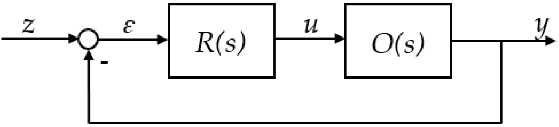
Figure 2.
Robustness reserve border A’OB’ of lower index ms.
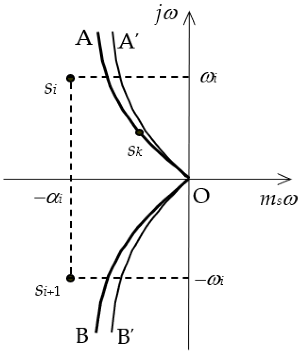
Figure 3.
Illustration of Integral square error (ISE).
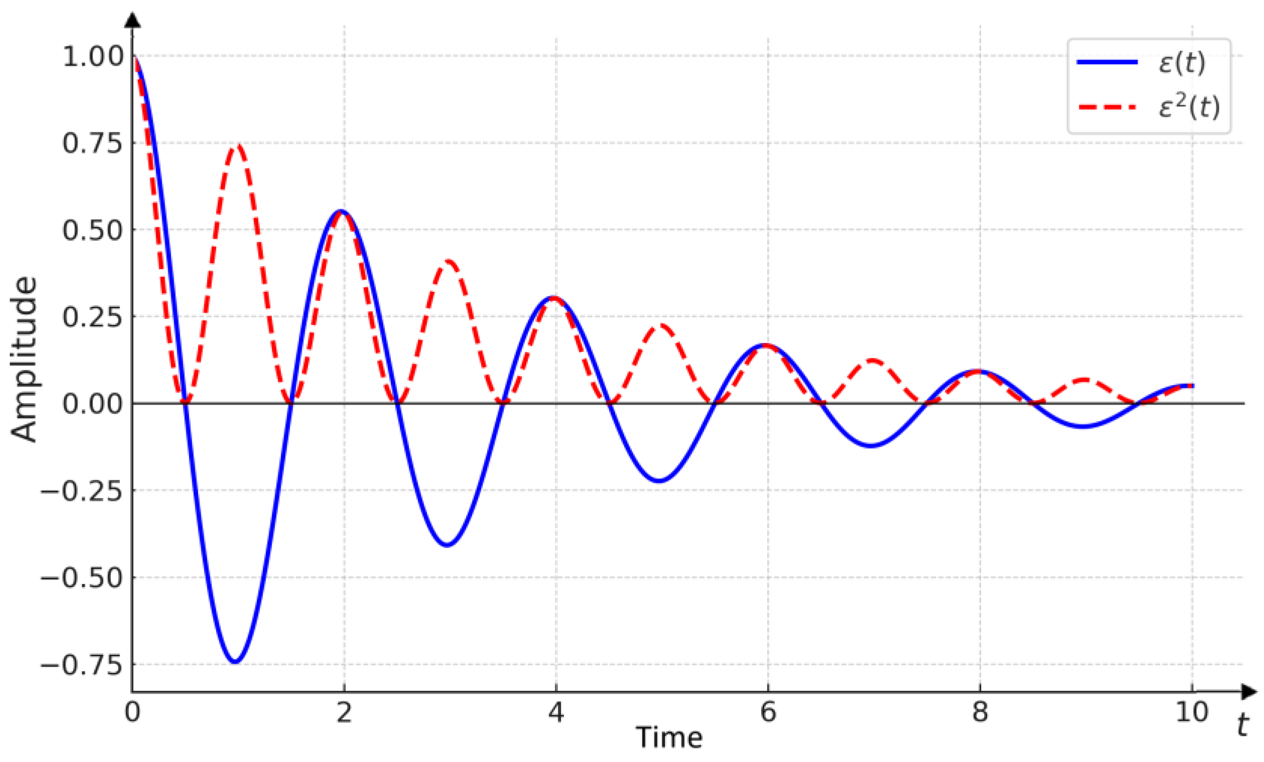
Figure 4.
Characteristics of the function f(x).
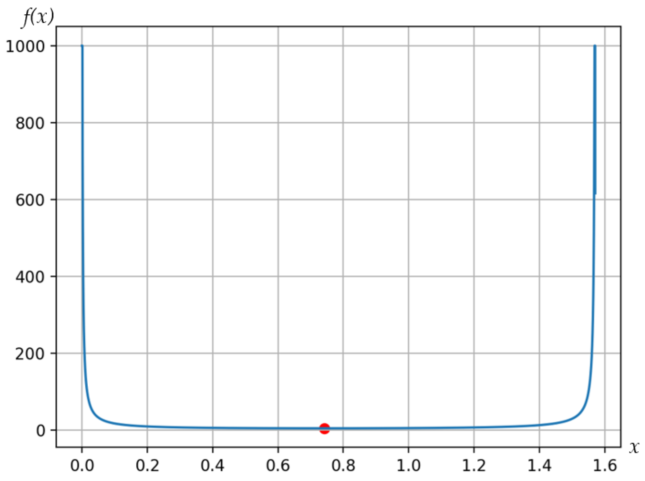
Figure 5.
Closed-loop responses of , and .
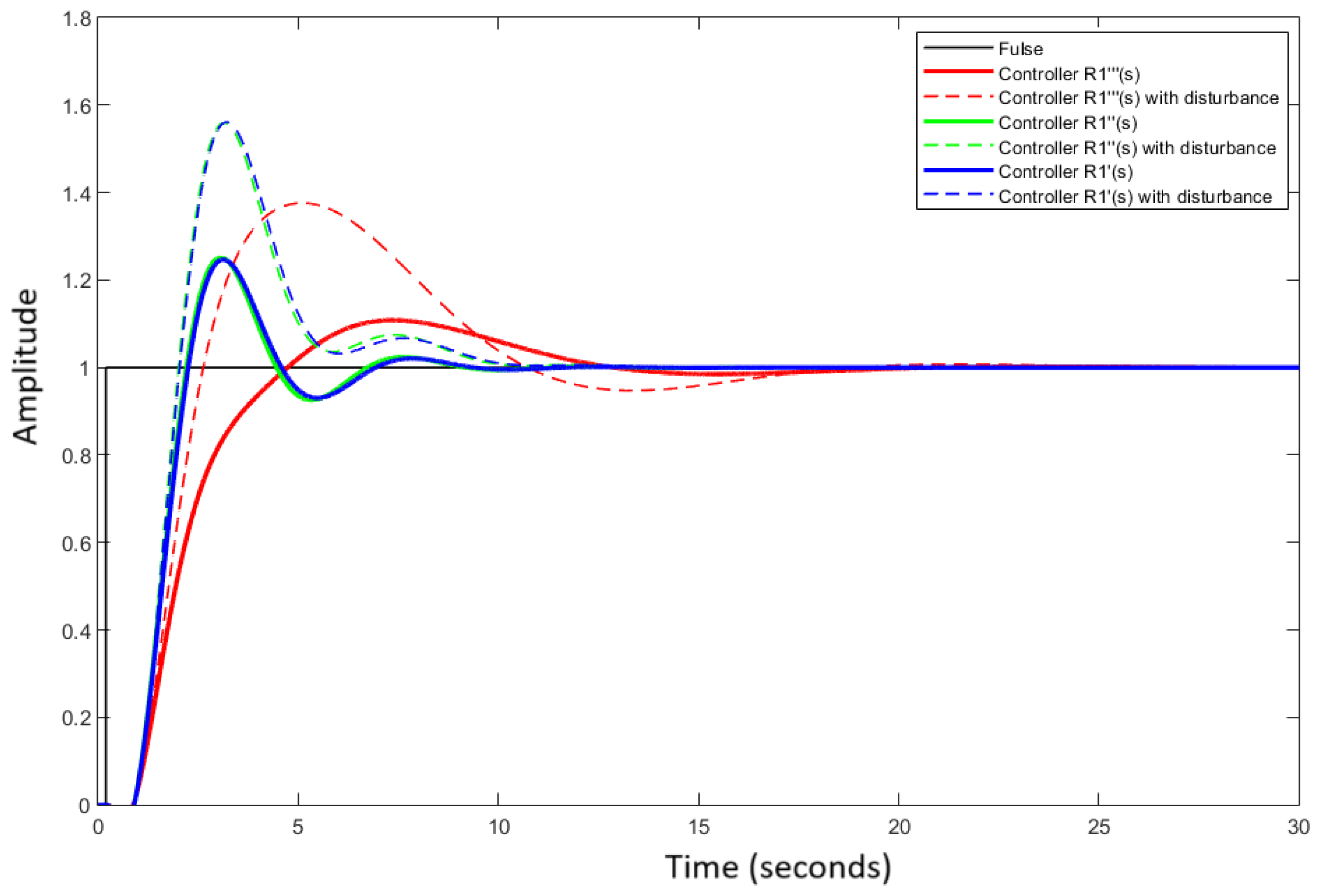
Figure 6.
Unit step responses of O2(s).
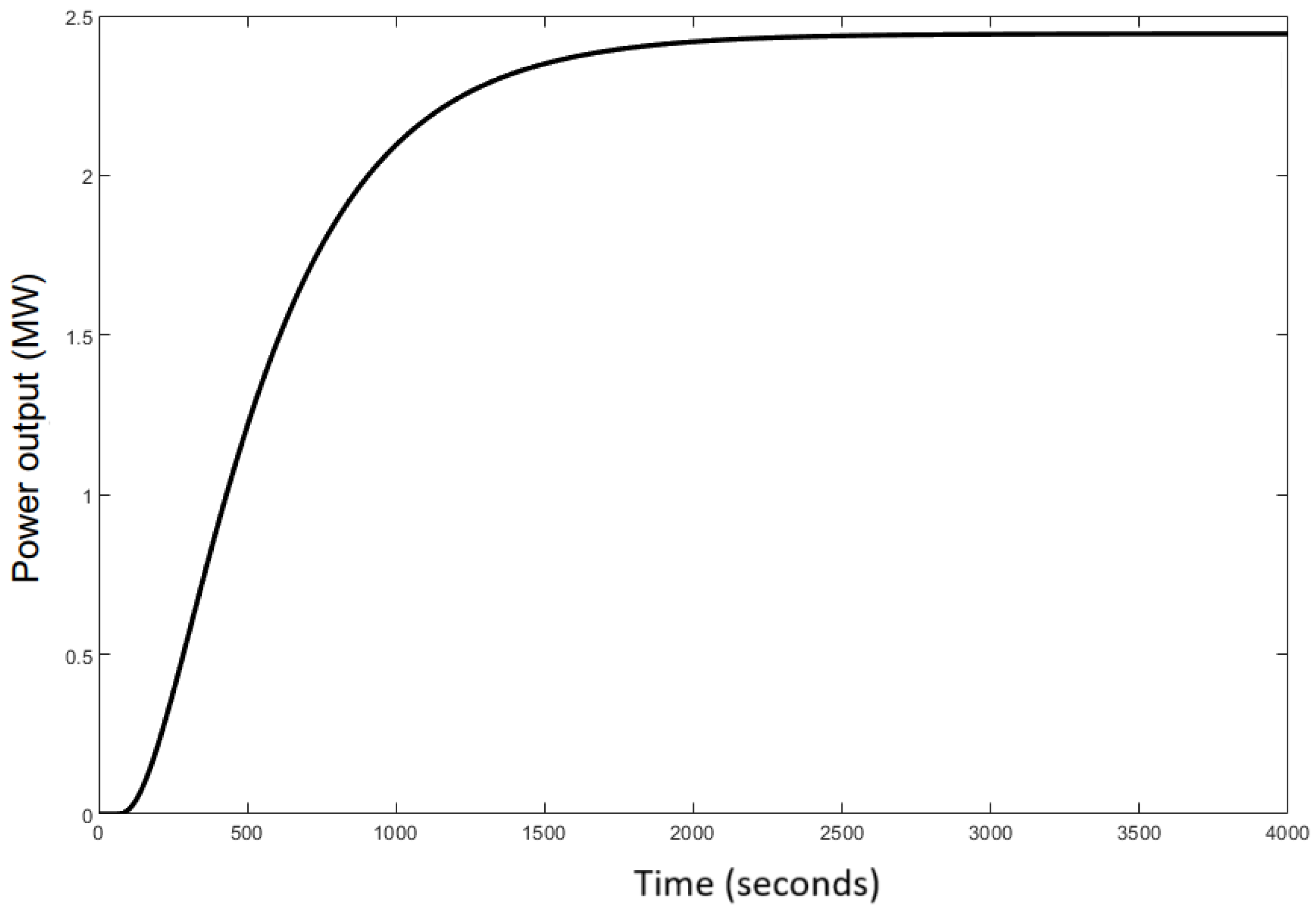
Figure 7.
Unit step responses of O2(s) and .
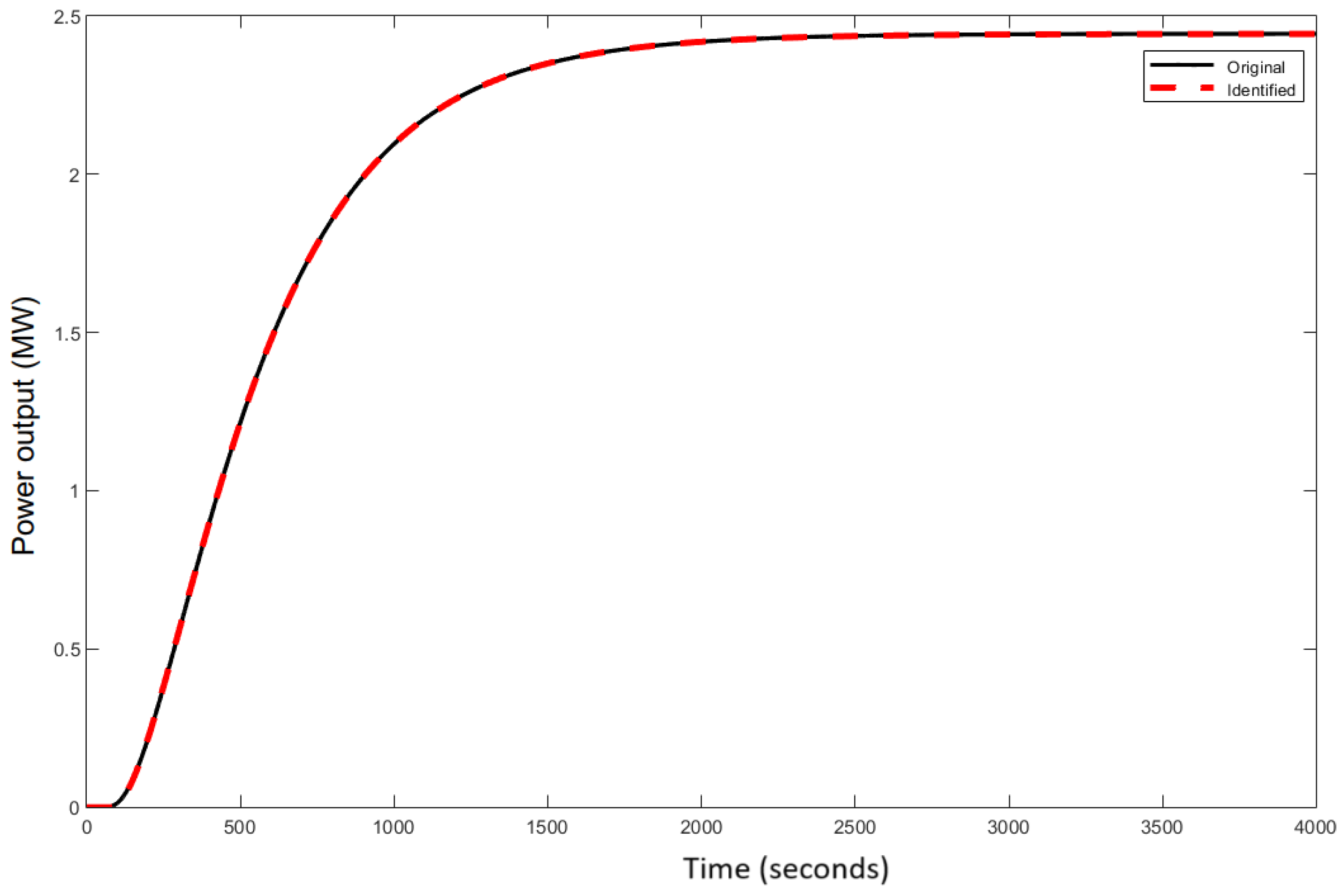
Figure 8.
Unit step responses of O2(s) closed-loop.
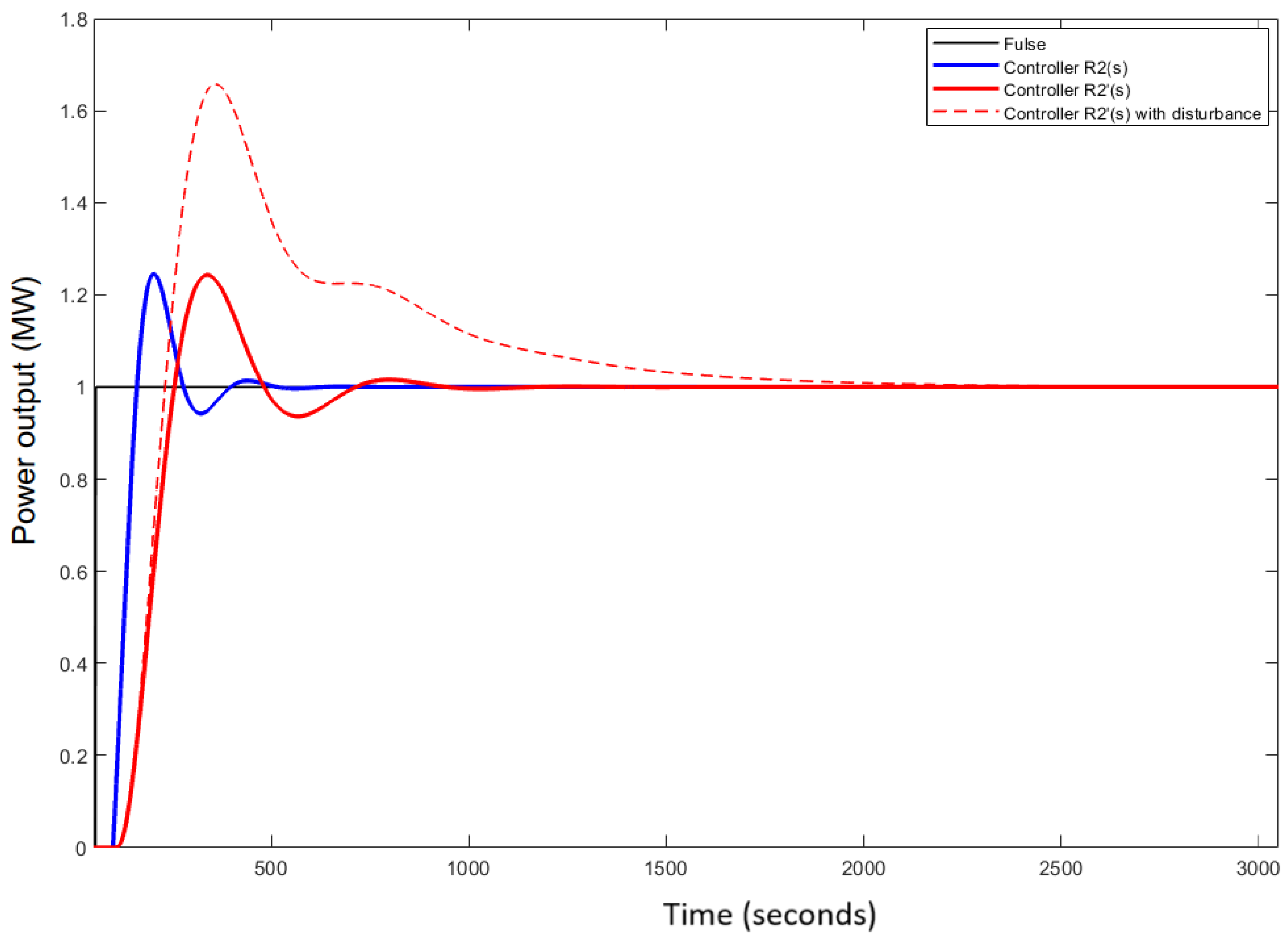
Table 1.
The main factors are based on the value of x.
| x | ms | J2(x) | θ | R(s) |
|---|---|---|---|---|
| 0.2 | 73,170.304 | 2.872τ | 5.000τ | |
| 0.4 | 2.318 | 1.701τ | 2.500τ | |
| 0.6 | 0.696 | 1.394τ | 1.667τ | |
| 0.742 | 0.461 | 1.345τ | 1.348τ | |
| 0.8 | 0.396 | 1.353τ | 1.250τ | |
| 1.0 | 0.238 | 1.513τ | τ | |
| 1.2 | 0.132 | 2.026τ | 0.833τ | |
| 1.4 | 0.054 | 3.970τ | 0.714τ |
Table 2.
The ratio of error to the minimum.
| x | ms | J2(x) | Rate to the Minimum (%) |
|---|---|---|---|
| 0.2 | 73,170.304 | 2.872τ | 214% |
| 0.4 | 2.318 | 1.701τ | 126% |
| 0.6 | 0.696 | 1.394τ | 104% |
| 0.742 | 0.461 | 1.345τ | 100% |
| 0.8 | 0.396 | 1.353τ | 101% |
| 1.0 | 0.238 | 1.513τ | 112% |
| 1.2 | 0.132 | 2.026τ | 151% |
| 1.4 | 0.054 | 3.970τ | 295% |
Table 3.
42 measuring points from O2(s) unit step response in summary.
| t1 | t2 | t3 | t4 | … | t41 | t42 |
| 0 | 40 | 140 | 240 | … | 3940 | 4040 |
| y1 | y2 | y3 | y4 | … | y41 | y42 |
| 0 | 0 | 0.0690 | 0.3476 | … | 2.4431 | 2.4431 |
Disclaimer/Publisher’s Note: The statements, opinions and data contained in all publications are solely those of the individual author(s) and contributor(s) and not of MDPI and/or the editor(s). MDPI and/or the editor(s) disclaim responsibility for any injury to people or property resulting from any ideas, methods, instructions or products referred to in the content. |
© 2025 by the authors. Licensee MDPI, Basel, Switzerland. This article is an open access article distributed under the terms and conditions of the Creative Commons Attribution (CC BY) license (http://creativecommons.org/licenses/by/4.0/).
Copyright: This open access article is published under a Creative Commons CC BY 4.0 license, which permit the free download, distribution, and reuse, provided that the author and preprint are cited in any reuse.


