
Submitted:
06 December 2024
Posted:
10 December 2024
You are already at the latest version
Abstract
Energy transfer stations (ETS) play a vital role in district cooling networks by facilitating thermal energy transfer between central chilled water plants and connected buildings. Effective control of ETS is crucial to maintain optimal temperature conditions and energy efficiency. However, traditional proportional-integral-derivative (PID) control may not always provide robust performance under changing operating conditions. This study aimed to evaluate and compare the control performances of PID, model predictive control (MPC), and fuzzy logic control (FLC) for an ETS process. A dynamic model of an ETS system incorporating a plate heat exchanger, control valve, temperature sensors and disturbances was developed. PID, MPC and FLC controllers were designed and tuned using the model. Controller performances were assessed through simulation-based experiments under setpoint changes and disturbances. Performance metrics such as rise time, settling time, overshoot, peak time and integral error were analyzed. Results showed that the MPC approach achieved the fastest rise time and lowest overshoot compared to PID and FLC. Meanwhile, FLC offered more robust control with minimal variations in performance metrics under changing conditions. Overall control effort was also lower with MPC and FLC. Proper selection of control strategy based on system requirements could help prevent issues like low delta-T syndrome in district cooling networks.
Keywords:
automation
; PID
; MPC
; fuzzy logic control
; PLC
; HMI
; heat exchanger
1. Introduction
District cooling systems have seen increasing adoption worldwide as an energy-efficient means of providing chilled water for space cooling and process requirements in large buildings, campuses and city centers [1]. A key component enabling district cooling networks are energy transfer stations (ETS), which act as intermediaries for thermal energy exchange between central chilled water plants and connected facilities [2]. Effective operation and control of ETS is important to reliably meet end-user cooling demands while maintaining optimum system efficiencies.
Poor control of ETS processes can lead to operational issues like low temperature differential (delta-T) between supply and return water streams [3]. Low delta-T severely impacts heat transfer capability within ETS heat exchangers, necessitating oversized equipment or excessive pumping power to achieve rated cooling capacities [4]. This reduces the overall energy efficiency of district cooling systems. Other issues stemming from inadequate ETS control include unstable temperature regulation, sluggish response to changing loads and overshooting/undershooting of setpoints [5]. Such control challenges are commonly tackled using conventional proportional-integral-derivative (PID) algorithms.
However, PID control may face limitations in complex, dynamically varying processes due to its non-predictive nature [6]. Model predictive control (MPC) and fuzzy logic control (FLC) are alternative techniques gaining popularity in industrial applications owing to their greater flexibility and robustness [7,8]. By incorporating dynamic process models, MPC can predict future behavior and optimize control actions accordingly [9]. Meanwhile, FLC mimics human decision making through fuzzy rule sets, facilitating control of nonlinear systems [10]. Both approaches show potential to address shortcomings of PID for ETS applications.
Low Delta T syndrome is a commonly observed issue in ETS characterized by a significant reduction in the temperature differential (ΔT) between the supply and return water in the district heating or cooling system compared to the expected or desired values. In an efficient and properly constructed ETS station, the hot supply water should have a considerably higher temperature than the return water to effectively transfer energy to the building’s interior heating and cooling systems. However, when the ΔT decreases to an inadequate level, it indicates an imbalance in the system, which can lead to various complications.
A reduced ΔT value indicates a decrease in the amount of heat exchange occurring at the ETS station, resulting in a decline in energy transfer efficiency. Consequently, more energy is required to maintain the desired heating and cooling levels in the connected buildings. To compensate for the low ΔT, the ETS station may need to operate its heating or cooling equipment at higher power levels or for longer durations. This increased energy consumption can lead to higher operating expenses. Additionally, the pumping system may need to work harder to maintain the required flow rates and counteract the effects of low ΔT, resulting in increased power consumption and operating costs.
An ETS control system consists of actuators such as pumps and control valves, sensors that monitor temperature and flow rates, controllers that supervise system operations, and an HMI (Human-Machine Interface) that facilitates operator contact. Data sharing is made possible via a communication network, and energy usage optimization is improved by variable frequency drives. It is crucial to ensure that the control system, measurement sensors, and final control elements are appropriately chosen, sized, and calibrated to prevent the occurrence of a low delta-T condition, which can be anticipated if these factors are not adequately addressed.
Heat exchangers play a crucial role in transmitting energy between the supply and return water. The control system can enhance energy transfer and increase ΔT by adjusting the operation of heat exchangers, such as modifying their heat transfer surface or capacity.
In an ETS station, the settling time, peak time, percentage overshoot, and associated control parameters work synergistically to influence the prevalence and severity of low delta T syndrome. The settling time directly affects how quickly the system stabilizes after a disruption or change in cooling demand. If the settling time is too long, there may be delayed system responses and extended periods before settling, resulting in ineffective cooling and potential inconvenience to the end user. On the other hand, a transient response time that is too short can lead to hasty and excessive control processes, which can cause oscillations and unpredictable temperature differences.
The peak time indicates the duration of temperature changes until the control response reaches its first peak. Excessive overshoot, where the temperature significantly exceeds the required difference before settling down, can be caused by an incorrectly chosen peak time. Low delta T syndrome is often caused by excessive overshoot, as it induces irregular temperature fluctuations and adversely affects the overall stability and energy efficiency of the system. Insufficient peak time can result in sluggish control responses, making it impossible to achieve the correct ΔT quickly.
This study aims to comparatively evaluate PID, MPC and FLC for controlling a simulated ETS process. A dynamic model incorporating key components is developed. Controller design and tuning are carried out. Performance under setpoint and disturbance scenarios is assessed using standard metrics to identify the most suitable strategy. Findings provide guidelines on selection of advanced control methods for improved ETS operation and district cooling system efficiencies.
The methodology employed in this study is detailed in Section 2. This includes process modelling activities to develop transfer functions representing the ETS heat exchanger, control valves and temperature sensors. Section 3 describes the design and tuning of the PID, MPC and FLC controllers based on the dynamic model. Simulation experiments and their results are presented in Section 4. Key performance metrics such as rise time, settling time, overshoot and error indices are analyzed from response and error plots. A comparative evaluation of the controllers is then conducted in Section 5 based on the aforementioned metrics under different operating scenarios. The concluding Section 6 summarizes findings from the comparative study, outlines limitations and makes recommendations for further work.
2. Material and Methods
2.1. Chilled water plant and energy transfer station model
To study the control of an energy transfer station (ETS), a simulation model of a chilled water plant supplying an ETS was developed using MATLAB/Simulink. The chilled water plant was modeled as a chilled water supply with varying temperature to represent the fluctuations from the central plant. The ETS was modeled as a heat exchanger transferring energy between the primary chilled water supply and secondary chilled water loop supplying buildings. A ETS Programmable Logic Controller (PLC) system architecture has been designed in structured framework in line with ISA-95 guidelines [21] to effectively regulate and manage the distribution [20]. Figure 1 below shows PLC based control system architecture for the ETS station.
2.2. Heat exchanger
A plate heat exchanger was selected to model the heat exchanger in the ETS based on its ability to achieve near-temperature temperature differences required for chilled water applications. The heat exchanger was sized based on the design conditions of the chilled water plant using effectiveness-NTU method. Alfalaval sizing program is used to size the heat exchanger [25]. The specifications and sizing calculations are shown in Table 1.
The mathematical modeling of plate heat exchangers is based on unsteady-state energy balance equations. Two common approaches are used to build the mathematical model. The first approach assumes a constant total heat transfer coefficient (U), simplifying the analysis. The second approach considers U as a variable dependent on the mass flow rate of the hot stream, adding complexity to the model. In this study, a constant U has been assumed for ease of computational implementation. The unsteady-state energy balance equations for the cold and hot plates are as follows, assuming a constant U.
Where subscripts p and s stands for primary and secondary.
Where, subscript s and p stands for secondary and primary, respectively.
By taking the Laplace transform, the above equations yield as below:
Where and are represented as below:
Substituting Equation (3) in (4), the equation given below yields:
From the values of and given above, the results are as follows:
By using these results in Equation (3), the outcome is as follows which represents the transfer function of heat exchanger:
The and are as follows:
The transfer function of the heat exchanger has been estimated based on the historical data collected from a typical ETS station and is given as below:
2.3. Control valves
The flow of chilled water in both the primary and secondary loops of the ETS was controlled using butterfly control valves. The valves were sized based on the design flow rates using characteristics curves provided by the manufacturer. The sizing calculations for the butterfly valve on the primary side are shown in Figure 2 and Figure 3. The calculations for valve on secondary side were similar. The actuators for the control valves were selected based on the required torque [22]. For a control valve with an actuator, the input to the control valve is an analog input in the form of 4 to 20 m. A signal while the output is the flow rate. In addition, Figure 4. depicts sizing calculation of the actuator and Figure 5 shows control valve data acquisition loop.
The control valve gain is contingent upon the positioning of the butterfly control valve in relation to the output of the controller output. This relation is expressed in the equations below:
=Butterfly control valve gain
=Analog control signal from the controller
=Butterfly control valve position
= Flow coefficient
=Flow rate on the outlet of the Valve
The control valve dependency on the term a relationship of the fraction of butterfly valve position and the percentage of the controller output as expressed in below equation:
=Fraction of butterfly valve position
When the butterfly valve is in fail to close configuration, the positive (+) sign comes into picture, otherwise the negative (–) sign is considered.
The two features that are often employed to control flow are linear and equal percentage characteristics as described in the equations below:
The below equation has been considered in this project where the nonlinear exponential function has been linearized.
A control valve’s flow coefficient, pressure drop across the valve as well as the fluid characteristics play a role in determining how much fluid flows through it. The following equation may be used to explain the link between the flow rate and the value.
stands for the pressure drop across the valve, or the pressure differential between the valve’s intake and exit and is the fluid’s density.
As the control valve selected for this project is equal percentage, the gain of the control valve can be represented as follows:
2.4. Sensors
Temperature indicating transmitters (TITs) were used to measure the temperatures at the inlet and outlet of the primary and secondary sides of the heat exchanger. The TITs had an accuracy of ±0.1°C and response time of 5 seconds. Magnetic flow meters were used to measure the flow rates on both sides with an accuracy of ±1% of reading. The measurements are conducted by means of a Resistance Temperature Detector (RTD), which serves as a temperature sensor.
To accomplish this, an RTD sensor is employed, which undergoes alterations in resistance in response to temperature fluctuations. The form of the first-order transfer function is as below:
The output current represented by the Laplace transform , is related to the input temperature represented by the Laplace transform , through the transfer function gain K and the system’s time constant τ.
For the above equation, t represents the temperature of RTD in degrees Celsius. The resistance of the RTD can be represented by the function RTD (t), where ‘t’ signifies the temperature of the RTD. The value represents the resistance of the RTD at 0 degrees Celsius, typically 100Ω. Additionally, two constants are involved: A, which equals 3.9083 × °C, and B, which equals –5.775 × °C respectively.
By introducing the transmitter gain to the transfer function calculated using MATLAB, we get the transfer function of the temperature transmitter as below:
2.5. Controllers
Control strategies play a crucial role in regulating the temperature and achieving accurate setpoint tracking in a ETS. In this study, we explore different control approaches for ETS, including classical and modern methods. The classical control method employed is the PID control, which is widely used in industrial applications. Additionally, we investigate two modern control methods: MPC and FLC. Figure 6 illustrates simulation of PID control, while Figure 7 illustrates simulation model of MPC control strategy. Figure 8 showcases the simulation diagram of FLC control. These control strategies will be evaluated and compared based on their effectiveness in regulating the building’s temperature and achieving precise setpoint tracking. A PID controller, MPC controller and FLC were designed and tuned in MATLAB/Simulink environment to control the ETS process. The controllers manipulated the control valve position on the secondary side to track a temperature setpoint.
2.6. Disturbances
To simulate disturbances in the chilled water supply temperature, random variations were introduced to represent load changes at the central chilled water plant. In addition, variations in the fluid’s viscosity and thermal conductivity were considered, as they can affect the efficiency of the heat exchanger.
3. Methodology and Implementation
A dynamic model of the ETS process was developed using first principles to simulate the real system behaviour. Key components modelled include a plate heat exchanger (PHE), control valve, temperature sensors and external disturbances. Performance curves provided heat transfer coefficients and pressure drop characteristics of the PHE. Linear transfer functions with time constants modelled the temperature response at primary and secondary sides. Mass flow rate variations in the control valve were represented as a second-order lag function. Step responses of these individual component models were obtained.
3.1. System Model Development
A block diagram (Figure 9) depicts the overall ETS process model integrating the component models [23]. Mass flows on the primary and secondary sides were considered as inputs along with a disturbance. Temperatures at both sides of the PHE were outputs. The model was developed and simulated in MATLAB/Simulink environment.
3.2. Controller Design
PI values for the PID controller were manually tuned to obtain optimum response. The MPC algorithm predicted outputs over a horizon using the process model, optimized control actions through minimization of a cost function. FIS variables were fuzzified using triangular membership functions. A rule base mimicked operator control decisions.
3.3. Simulation Experiments
Controller responses to setpoint changes, load disturbances and parametric variations were assessed. Simulation time was set sufficiently high to capture transients. Data obtained from simulations included temperature and mass flow trajectories, control efforts. Metrics such as rise time, settling time, peak overshoot were automatically computed.
3.4. Performance Evaluation
The different controllers were compared using the simulation results and performance metrics. Effectiveness, robustness and relative computational requirements were evaluated to identify the most suitable control strategy for ETS applications.
3.5. Controller Design and Tuning
3.5.1. PID Controller
A PID controller was designed using the process model developed in Simulink. The controller input was selected as the temperature error (set-point - measured temperature). The output acted as a control signal for the control valve flow adjustment.
Manual tuning was performed to determine optimal PID parameters. Initially, proportional gain (Kp) was increased from 0 until oscillations were observed, then reduced slightly. Integrator gain (Ki) was increased slowly until the settling time decreased without overshoot. Derivator gain (Kd) was set to zero, then increased carefully to reduce rise time if no instability resulted. The parameter tuning process was repetitive until the quickest response time and minimal IAE were achieved.
3.6. MPC Controller
For MPC design, the prediction model consisted of discretized process model transfer functions over the prediction horizon (Hp). Control horizon (Hc) was selected as one time-step. A Quadratic objective function minimized errors and control efforts within constraints. To solve the optimization problem at each sampling instant, an Interior Point solver from the MPC Toolbox was used.
MPC parameters were tuned iteratively: Hp=5, Hc=1 and sampling time (Ts) of 1 second resulted in good response without constraint violations. Weighting matrices Q and R were adjusted to achieve balanced error reduction and smooth control effort.
3.7. Fuzzy Logic Controller
A three-input, single-output Mamdani type FLC was designed in Simulink. Inputs were error (e) and change in error (de/dt) signals. The output was the control signal to the valve. Triangular membership functions were used after numerous design iterations. A 24-rule IF-THEN control rule base was formulated based on expert knowledge and centroid defuzzification was employed. The controller parameters were tuned experimentally to achieve minimal overshoot and fast settling time.
4. Results and Benchmarking
4.1. Open-loop Response
Plant behaviour under an inputs step was observed first (Figure 10). A peak temperature deviation of 0.8°C occurred at 80s due to process dynamics before stabilizing. This served as the benchmark for assessing controller performances.
4.2. PID Controller Response
Figure 11 depicts a rise time of 1.37 indicates that after a step change in the reference signal, the system reaches a certain percentage (often 90% or 95%) of its final value at approximately 1.37 units of time. Likewise, a settling time of 45.13 means that the system stabilizes within the defined tolerance zone in approximately 45.13 time-units. The system initially exhibits an overshoot of approximately 27.6 percent before approaching target. What is noteworthy is that no undershoot is observed in this particular response, indicating that the system does not fall below the setpoint after reaching the setpoint. In this specific case, the system reaches a peak value of approximately 1.28. The maximum deviation from the setpoint is likely to be reached by the system which is indicated by a peak time of 4.9344 time-units. These control parameters are shown in Table 2.
Rise time is the time taken for the output to reach 99% of the final value during response to a step change. As seen in Table 2, PID has the lowest rise time of 1.3s compared to 2.49s for FLC and 12.6s for MPC. Settling time is the time required for the output to settle within 2% of the final value. MPC exhibited the fastest settling of 32s, followed by PID at 45s and FLC at 61s. Percentage overshoot indicates the maximum temperature excursion beyond the setpoint. MPC had no overshoot while FLC and PID has overshoot. In comparison, the PID response manifested higher overshoot.
4.3. MPC Controller Response
The step response of the MPC controller is shown in Figure 12. A rise time of 14.6123 indicates that after a step change in the reference signal, the system reaches a certain percentage (often 90% or 95%) of its final value at approximately 0.5853 units of time. Likewise, a settling time of 32.9513 means that the system stabilizes within the defined tolerance zone in approximately 32.9513-time units. What is noteworthy is that no overshoot or undershoot is observed in this particular response, indicating that the system does not fall below the setpoint after reaching the setpoint. In this specific case, the system reaches a peak value of approximately 1.0017. The maximum deviation from the setpoint is likely to be reached by the system after approximately 200-time units after a step change. These control parameters are shown in Table 2.
4.4. Fuzzy Logic Controller Response
Figure 13 illustrates the FLC response, for the step response of the FLC controller. The rise time is quantified as 2.49 seconds and refers to the time it takes for the system to return to its initial state after a disturbance. The investigation carried out revealed a settling time of 61.43 seconds and provides information about the time frame within which the system reaches a stable state within the intended tolerance range of 5%. The recorded value of 111.54% indicates an overshoot that exceeds the final result by 111.54%, highlighting the transient nature of the system. The peak value observed in this analysis is 2.11, indicating the maximum output signal during the system response. The precise measurement of 9.85 time units emphasizes the point at which the system reaches its highest response value, thus providing an explanation for the system’s erratic behavior. These parameters are summarized in Table 2.
4.5. Comparative Analysis
A stepwise comparison (Figure 14) revealed MPC as the superior controller with the fastest response (rise time 20s). FLC offered robust performance, settling 2-3X faster than PID. Integral error metrics ISE and IAE consistently ranked MPC above FLC and PID.
4.6. Comparative Evaluation
The controllers were evaluated based on relevant performance metrics:
4.7. Error Analysis
The integral error metrics ISE and IAE provide a quantitative measure of controller error. MPC consistently outperformed other controllers with the lowest errors, especially under disturbance scenarios (Figure 15).
4.8. Robustness
FLC demonstrated robustness to alterations in its design parameters like membership functions and rules. PID tended to become unstable more easily than MPC or FLC under similar variations.
4.9. Computational Load
The MATLAB CPU usage was lowest for PID at 1-2% compared to 5-7% for FLC and 10-12% for MPC. This agrees with their computational complexities.
MPC demonstrated the fastest and most accurate response, while FLC was more robust than PID. However, MPC imposed higher computational loads than FLC and PID controllers. Appropriate control strategy must be selected based on application requirements and available hardware resources.
5. Conclusions
This study compared the performances of PID, MPC and FLC techniques for controlling an ETS process. A dynamic model representing key components was developed. Controllers were designed based on this model and tuned experimentally. Simulation results revealed that MPC controlled the temperature most effectively with negligible rise time and overshoot. It consistently exhibited the lowest integral error metrics, indicating superior setpoint tracking ability. Its predictions based on a dynamic model allowed compensating future deviations optimally.
FLC offered robust control, settling 2-3 times faster than the conventional PID. It demonstrated resilience against parameter changes, making it a suitable alternative. However, overshoot and rise time were marginally higher than MPC.
While PID succeeded in stabilizing the process, its response was sluggish with noticeable overshoot. Tuning proved difficult due to interacting gains. Its performance deteriorated more than other algorithms under deviations. Computational expenses increased in the order of PID, FLC and MPC approaches. MPC necessitated greatest processing resources, restricting its applications to systems with high-performance controllers.
In view of these results, MPC shows promise as a primary control technique for ETS where precise temperature regulation is critical. FLC can substitute PID effectively if computing limitations exist. Selection depends on process characteristics and hardware capabilities. Future work may encompass optimization of fuzzy variables, evaluation under scheduling scenarios and analyses with distributed parameter models. Experimental validation on physical ETS hardware is also recommended. Deployment of advanced regulators like MPC and FLC improves ETS control, facilitating energy savings and reliable chilled water networks. Proper control strategy selection is key to minimizing low delta-T and enhancing system efficiencies.
References
- A. Almeida. Low delta-T syndrome diagnosis and correction for chilled water plants. Master dissertation, Texas A & M University, 2014.
- S. Taylor. Degrading chilled water plant delta-T: Causes and mitigation. ASHRAE Transactions; Atlanta Vol. 108, 2002.
- F.W. Yu, K.T. Chan, Environmental performance and economic analysis of all-variable speed chiller systems with load-based speed control, Applied Thermal Engineering, Vol. 29, Issues 8–9, pp. 1721-1729, 2009.
- M. Dai, X. Lu, P. Xu. Causes of low delta-T syndrome for chilled water systems in buildings. Journal of Building Engineering, Vol. 33, 2021.
- D. Gao, S.W. Wang, K. Shan, C.C. Yan. A system-level fault detection and diagnosis method for low delta-T syndrome in the complex HVAC systems, Applied Energy, Vol. 164, pp. 1028-1038, 2016.
- Gao, D. C., Wang, S., & Shan, K. (2016). In-situ implementation and evaluation of an online robust pump speed control strategy for avoiding low delta-T syndrome in complex chilled water systems of high-rise buildings. Applied energy, 171, 541-554.
- C. Yan, X. Yang, Y. Xu. Mathematical explanation and fault diagnosis of low delta-T syndrome in building chilled water systems. Buildings 8(7), 84, 2018.
- Li, S., Gao, J., Wei, Y., Zhang, H., Wang, L., & Miao, J. (2022, August). Temperature Control and Energy Saving System for Communication Base Station Based on Fuzzy PID Algorithm. In 2022 34th Chinese Control and Decision Conference (CCDC) (pp. 1702-1707). IEEE. [CrossRef]
- Le Sha, Ziwei Jiang, Hejiang Sun, A control strategy of heating system based on adaptive model predictive control, Energy, Volume 273, 2023, 127192, ISSN 0360-5442.
- Li Liu, Jun Liu, Zhifeng Chen, Zhongyang Jiang, Ming Pang, Yanshu Miao, Research on predictive control of energy saving for central heating based on echo state network, Energy Reports, Volume 9, Supplement 4, 2023, Pages 171-181.
- Pavel Tichý, Petr Šlechta, Francisco P. Maturana, Raymond J. Staron, Kenwood H. Hall, Vladimír Mařík, Fred M. Discenzo, Multi-agent technology for robust control of shipboard chilled water system, IFAC Proceedings Volumes, Volume 37, Issue 10, 2004, Pages 303-308, ISSN 1474-6670.
- Kane, M. B. , Lynch, J. P., & Zimmerman, A. T. (2011, August). Decentralized agent-based control of chilled water plants using wireless sensor and actuator networks. In 2011 4th International Symposium on Resilient Control Systems (pp. 131-136). IEEE. [CrossRef]
- Li, X. , Li, Y., Seem, J. E., & Li, P. (2012, June). Extremum seeking control of cooling tower for self-optimizing efficient operation of chilled water systems. In 2012 American Control Conference (ACC) (pp. 3396-3401). IEEE. [CrossRef]
- Ma, Y., Borrelli, F., Hencey, B., Coffey, B., Bengea, S., & Haves, P. (2011). Model predictive control for the operation of building cooling systems. IEEE Transactions on control systems technology, 20(3), 796-803. [CrossRef]
- Su, C. L. , & Yu, K. T. (2012, May). Evaluation of differential pressure setpoint of chilled water pumps in cleanroom HVAC systems for energy savings in high-tech industries. In 48th IEEE Industrial & Commercial Power Systems Conference (pp. 1-9). IEEE. [CrossRef]
- Mu, B. , Li, Y., Salsbury, T. I., & House, J. M. (2016, July). Optimization and sequencing of chilled-water plant based on extremum seeking control. In 2016 American Control Conference (ACC) (pp. 2373-2378). IEEE. [CrossRef]
- Sane, H. S. , Haugstetter, C., & Bortoff, S. A. (2006, June). Building HVAC control systems-role of controls and optimization. In 2006 American Control Conference (pp. 6-pp). IEEE. [CrossRef]
- Du, J., Zhang, X., & Song, C. (2011, July). Multi-PID control of Hammerstein systems with input multiplicity. In Proceedings of the 30th Chinese Control Conference (pp. 303-306). IEEE.
- A. A. Olama. District cooling theory and practice, CRC Press, 2017.
- P. N. Sands, I. Verhappen. A guide to the automation body of knowledge, 3rd Edition, International Society of Automation (ISA) press. 2018.
- Zafar, M., & Wei, B. (2023, June). Comparison Analysis of Thermistor and RTD for Energy Transfer Station Application. In 2023 IEEE/ASME International Conference on Advanced Intelligent Mechatronics (AIM) (pp. 800-805). IEEE. [CrossRef]
- Olama, A. A. (2016). District cooling: Theory and practice. CRC Press.
- Internet resource: Bray Control Valve Sizing URL: https://www.bray.com/valves-actuators-controls/control-valves/control-valves-sizing#gc-section-3 (accessed 05/28/2024).
- Internet resource: The Alfa Laval HEXpert Heat exchanger selector tool. Online heat exchanger selector tool. URL: https://www.alfalaval.com/products/heat-transfer/heat-exchanger-selector-tool/heat-exchanger-selector-tool/ (accessed 05/28/2024).
Figure 1.
PLC based control system architecture for the ETS station.
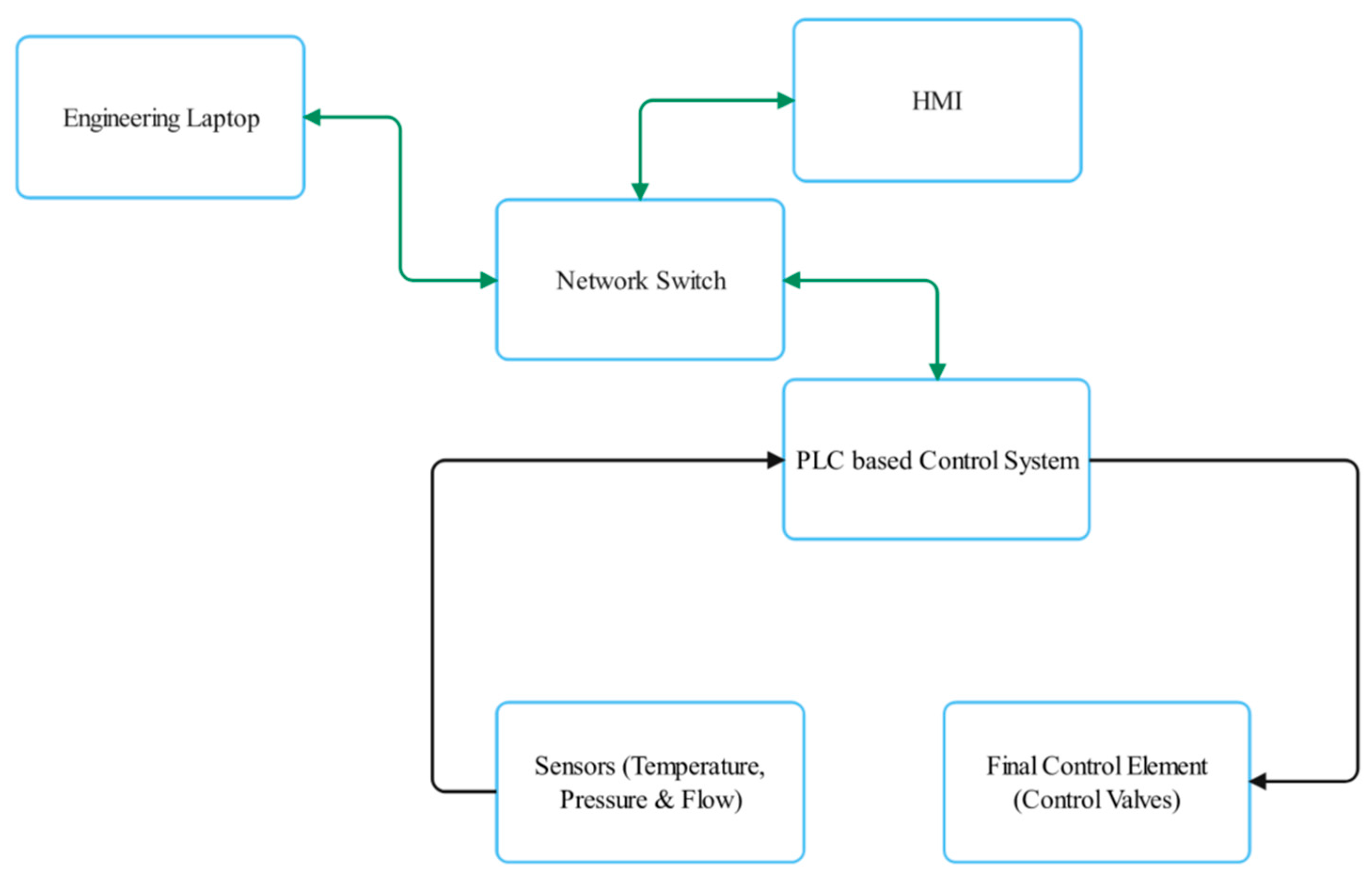
Figure 2.
Sizing calculation of the butterfly valve using Bray sizing program [24].
Figure 2.
Sizing calculation of the butterfly valve using Bray sizing program [24].
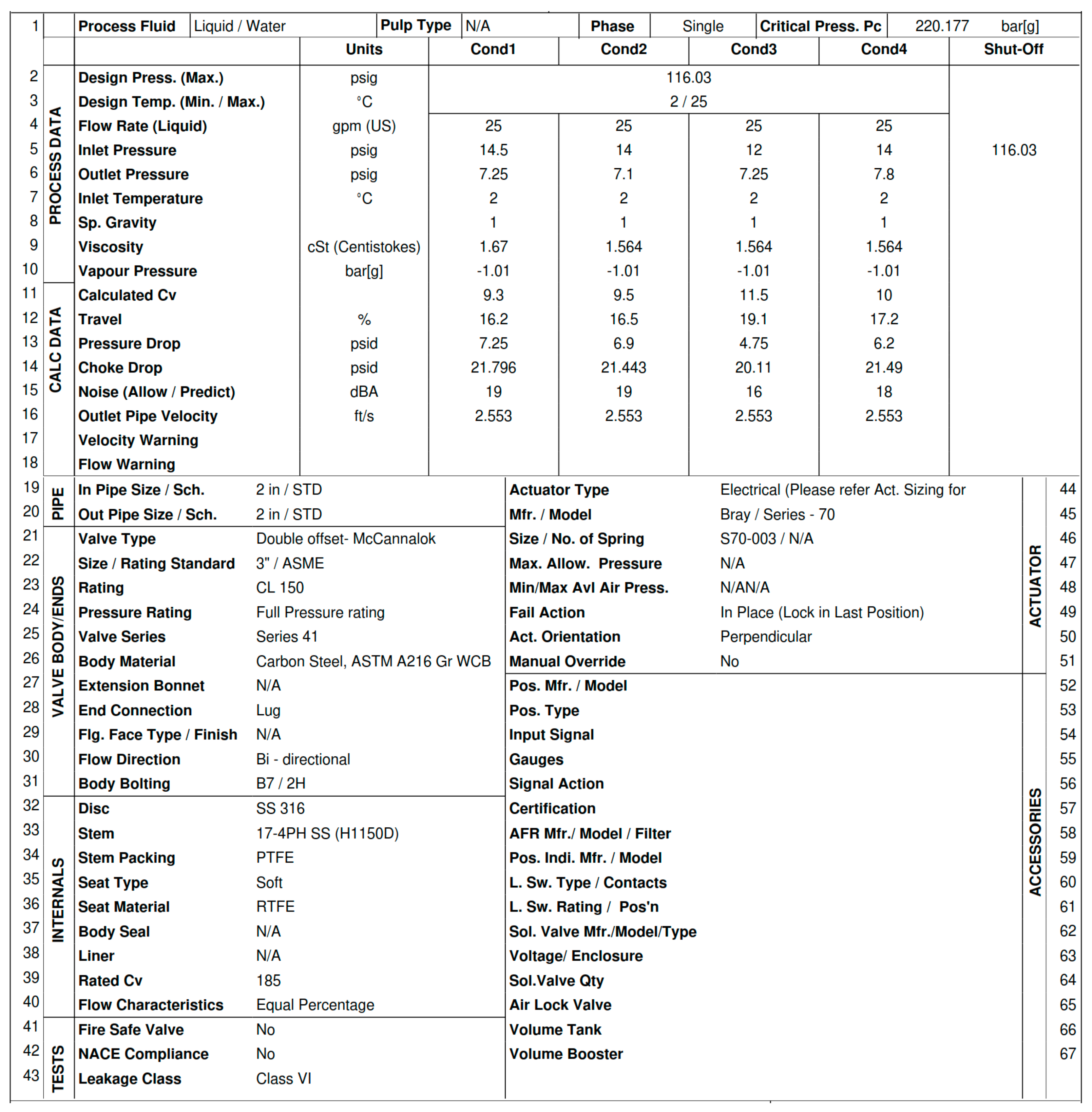
Figure 3.
Sizing calculation of the butterfly valve using Bray sizing program [24].
Figure 3.
Sizing calculation of the butterfly valve using Bray sizing program [24].
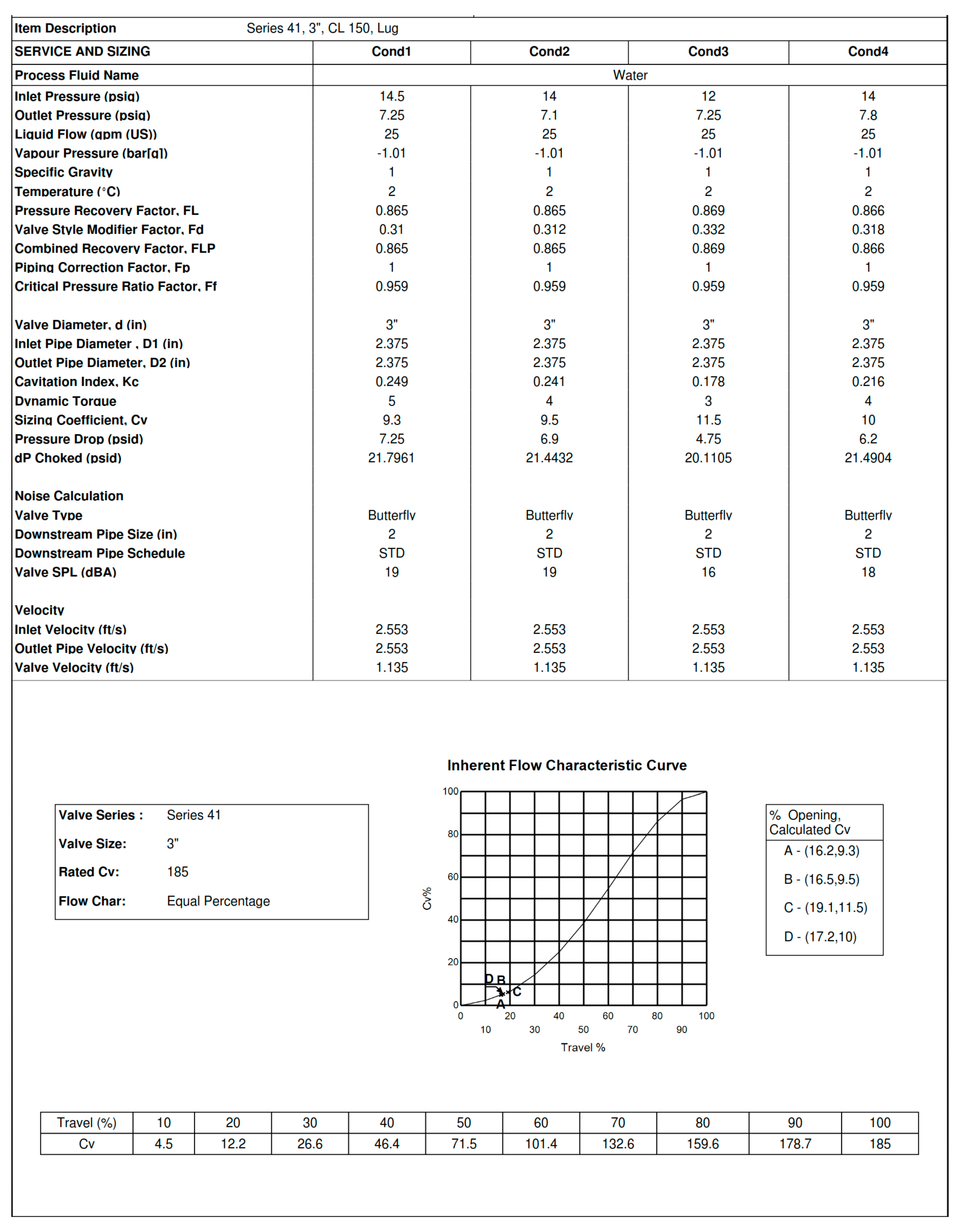
Figure 4.
Sizing calculation of the actuator using Bray sizing program [24].
Figure 4.
Sizing calculation of the actuator using Bray sizing program [24].
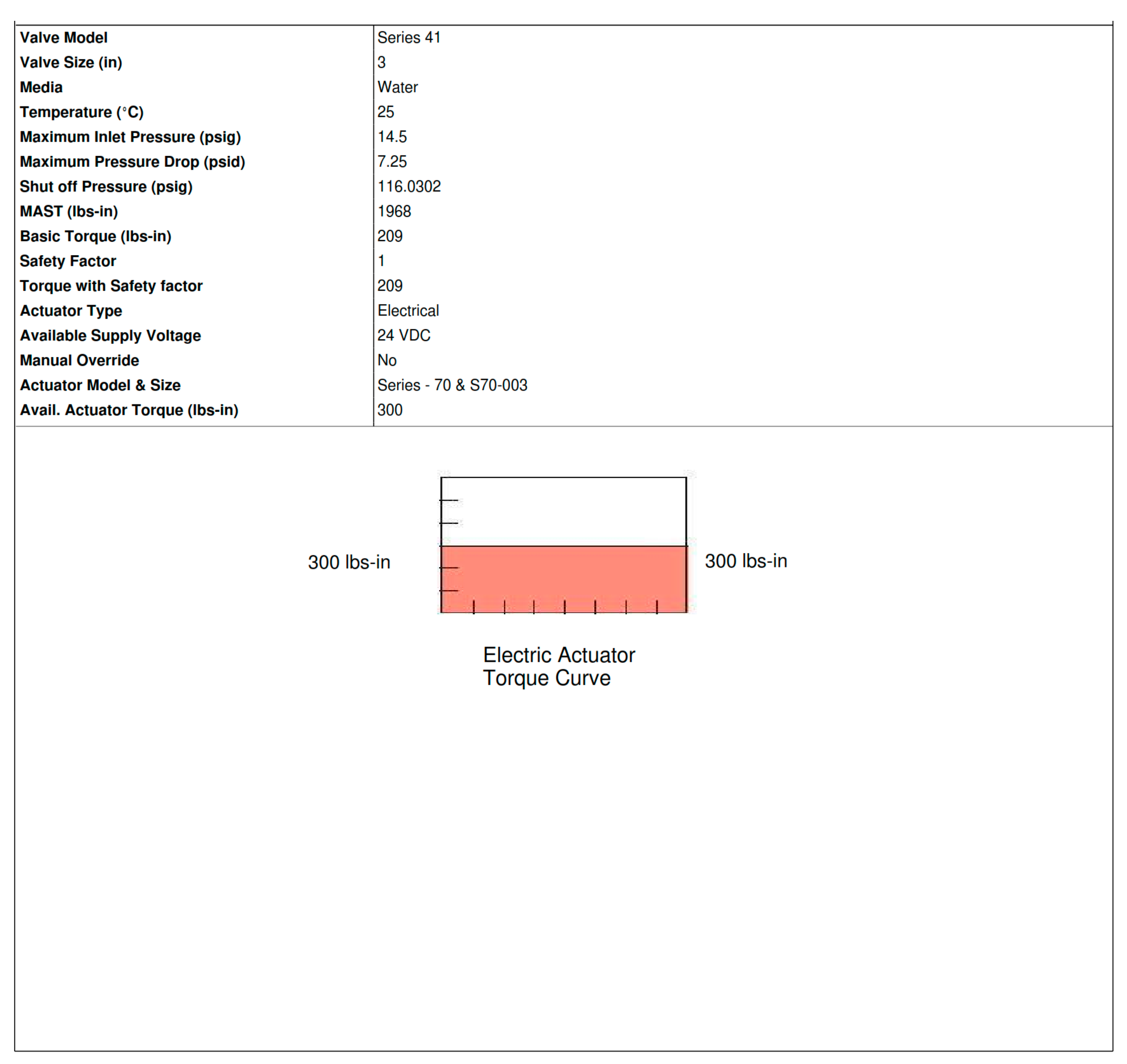
Figure 5.
Control valve data acquisition loop, source; authors own illustration.
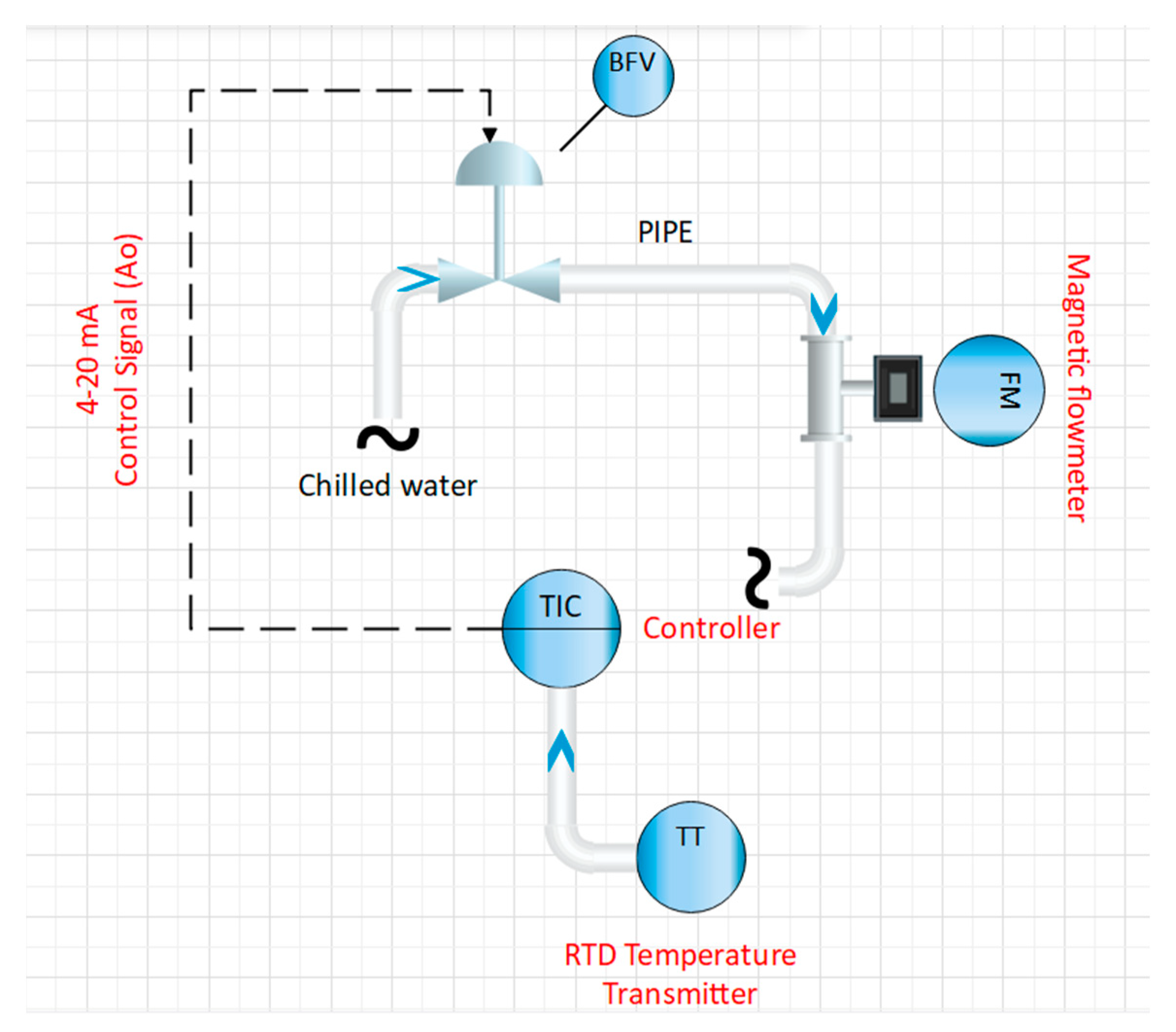
Figure 6.
Simulink model of PID control.
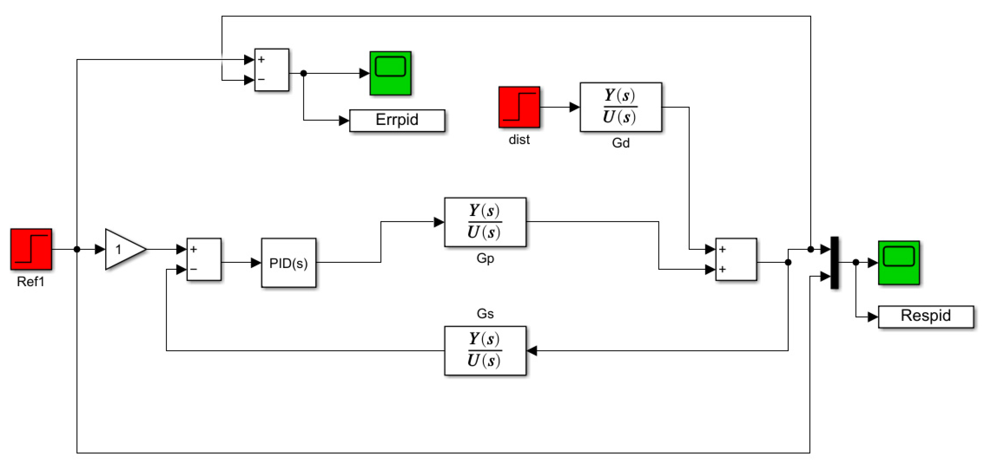
Figure 7.
Simulink Model of MPC Control.
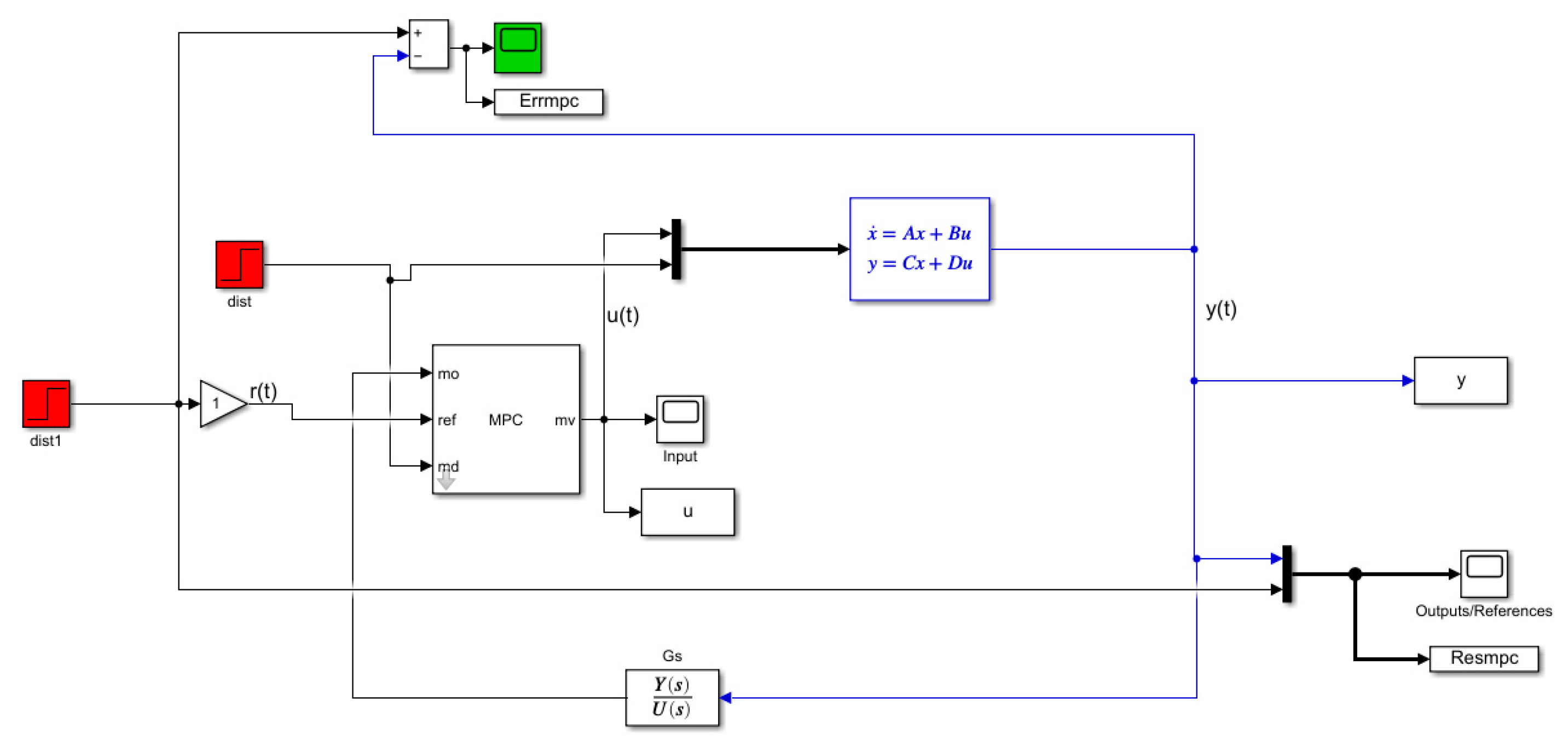
Figure 8.
Simulink diagram of FLC Control.
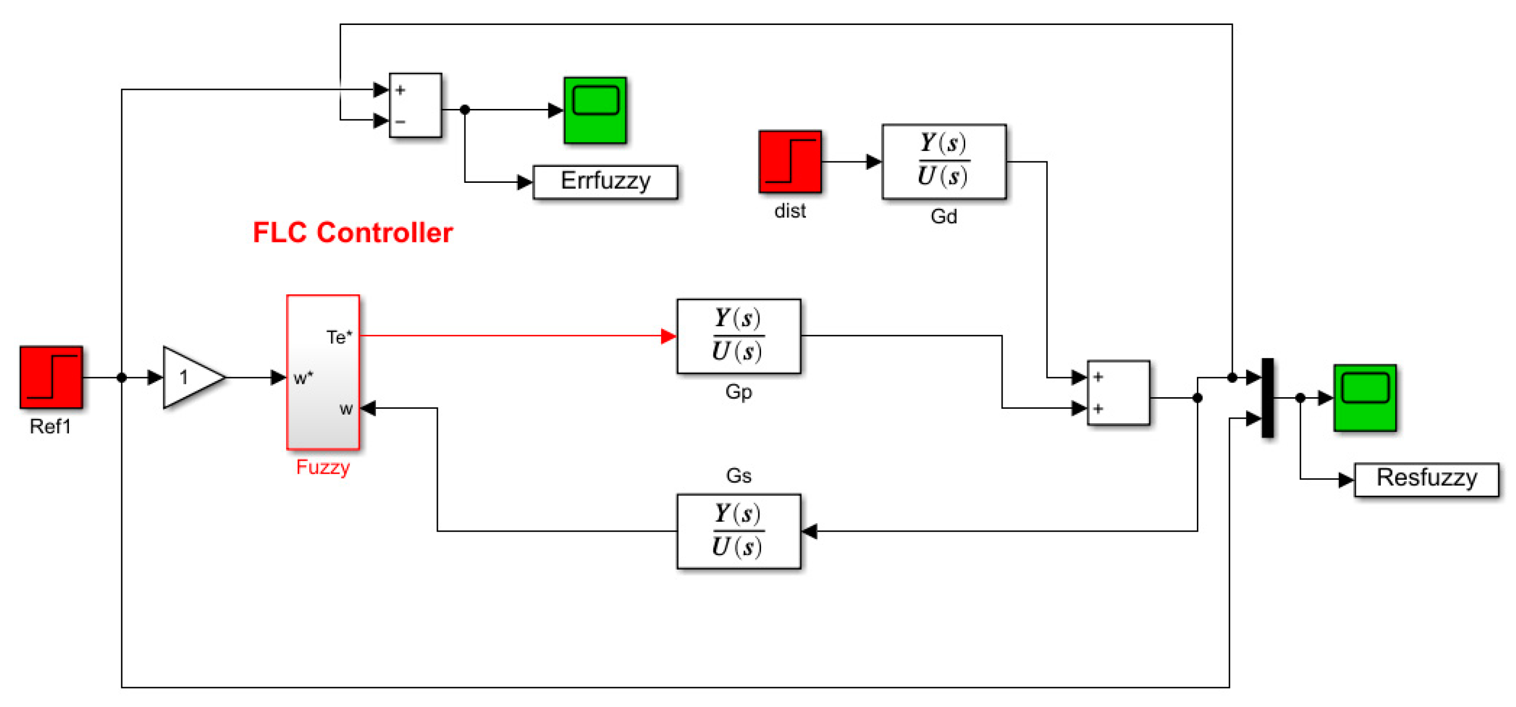
Figure 9.
Typical ETS control system.
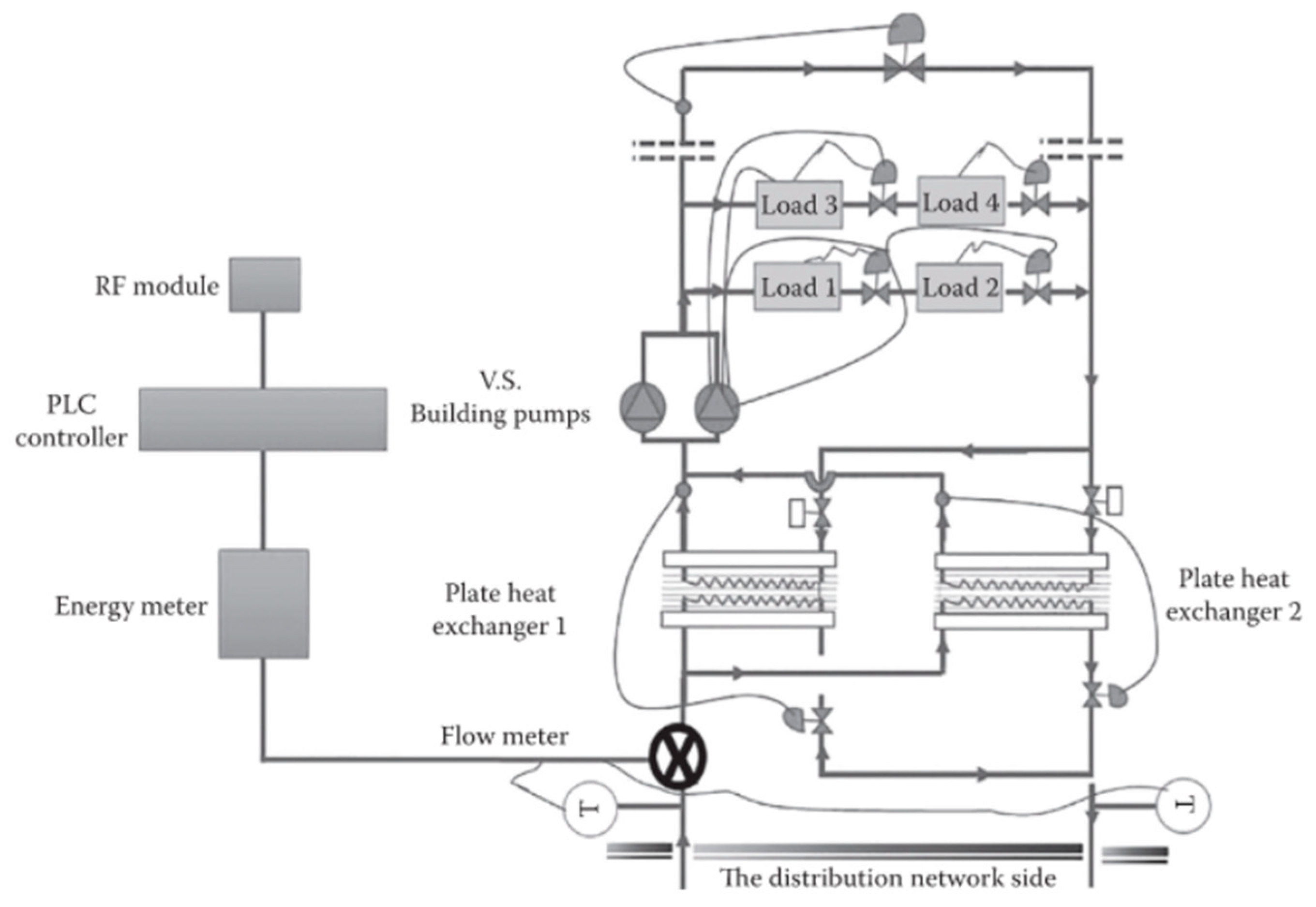
Figure 10.
Step response of ETS process .
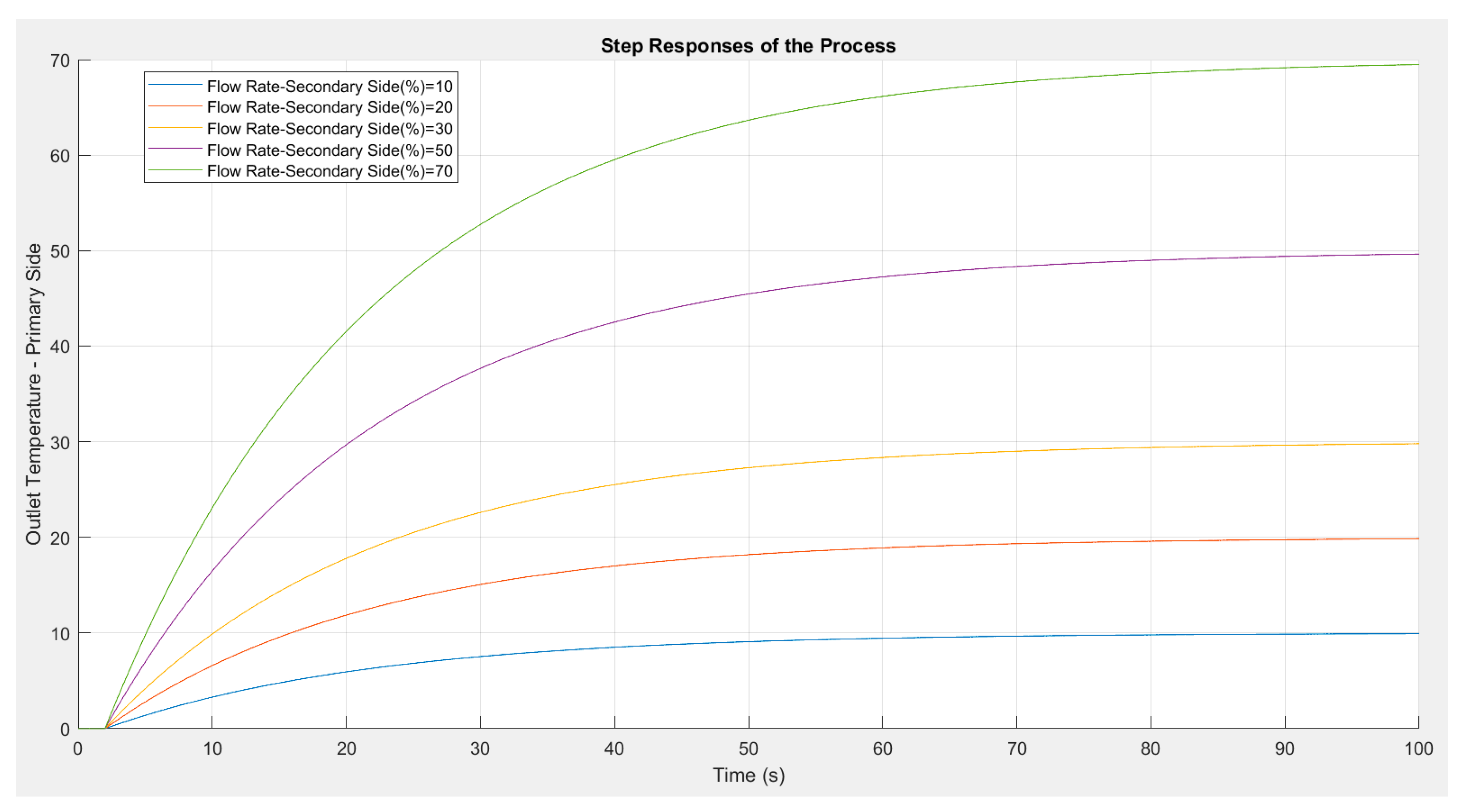
Figure 11.
Step response of PID controller.
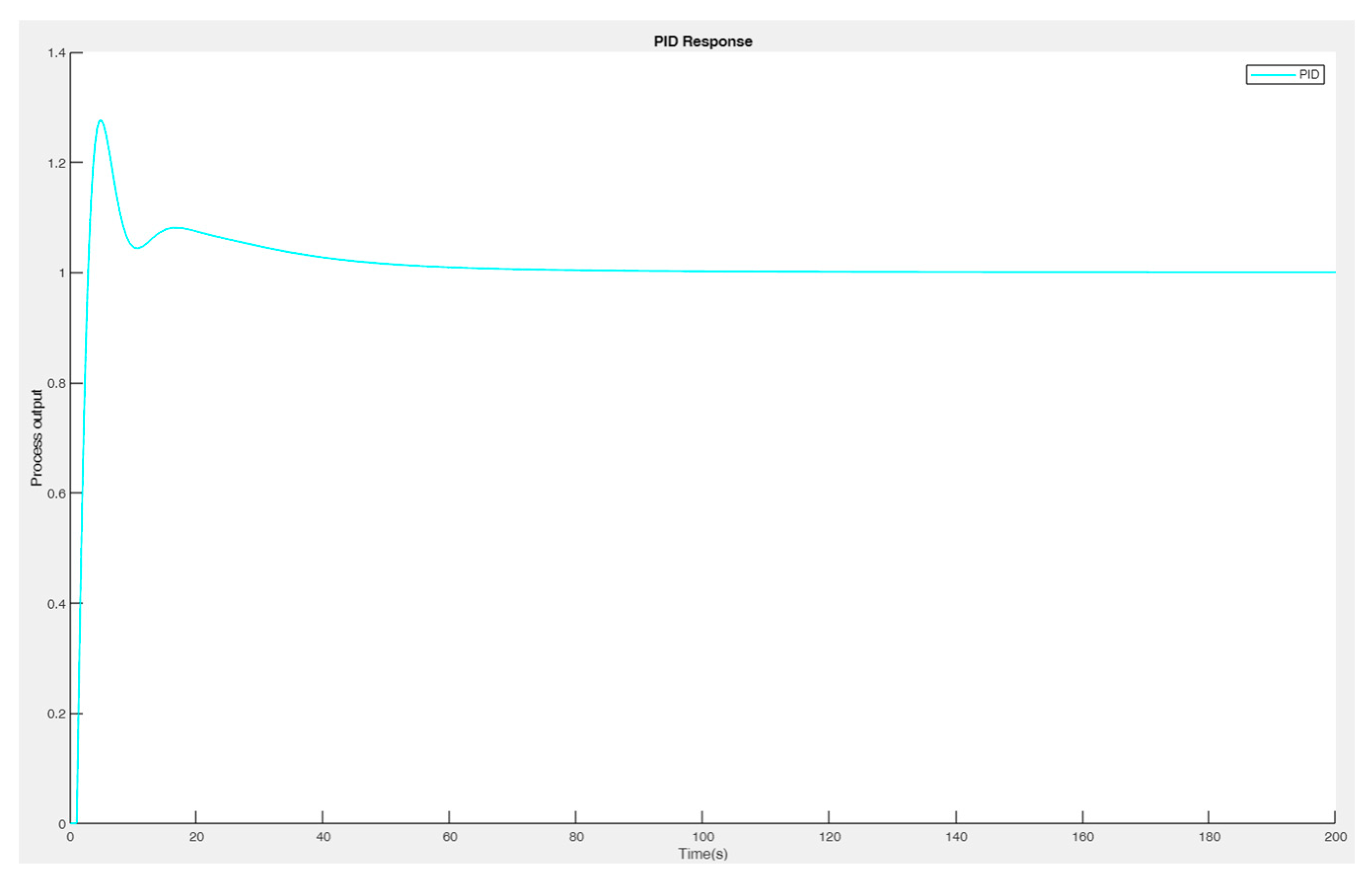
Figure 12.
Step response of MPC controller.
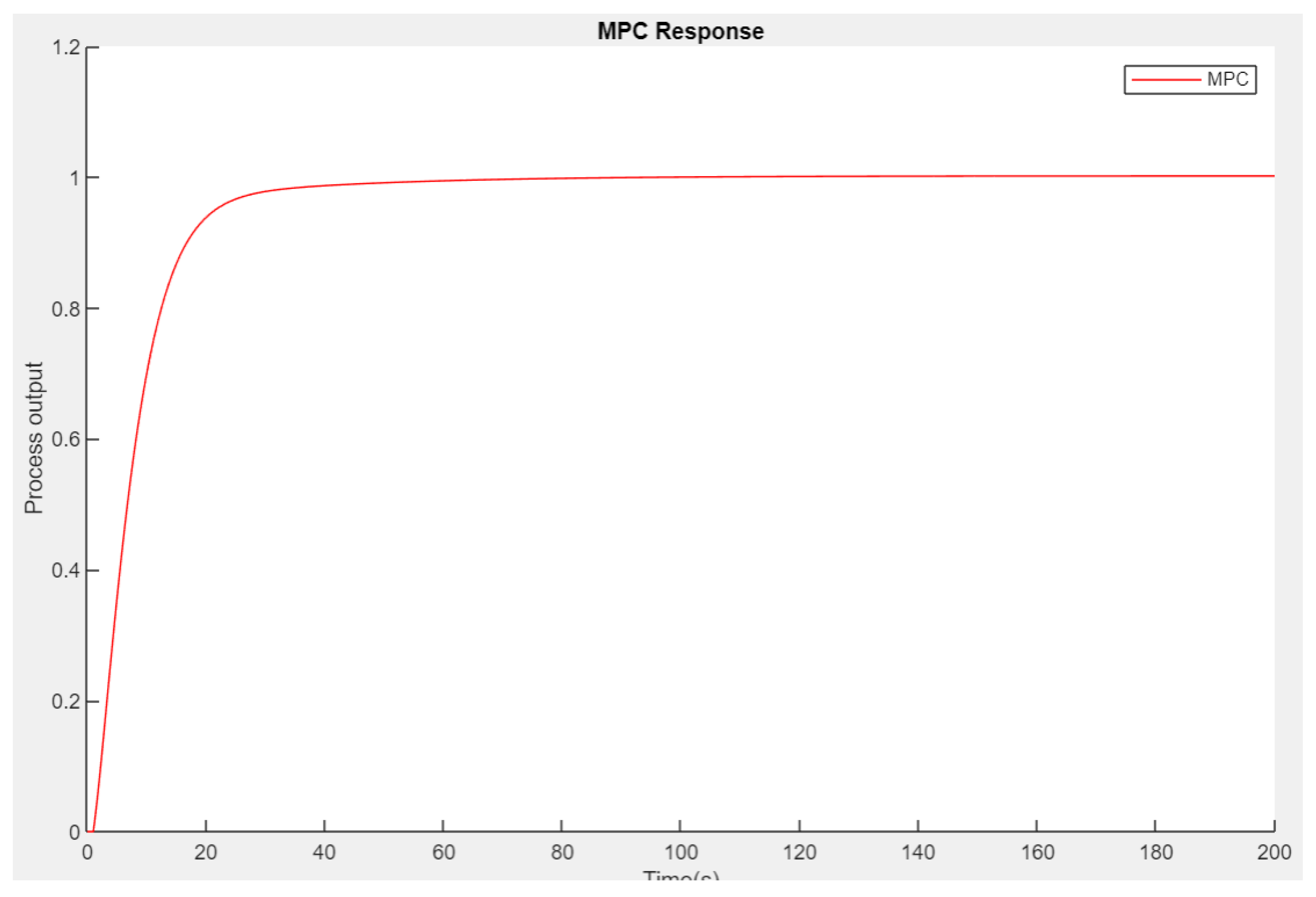
Figure 13.
Step response of FLC controller.
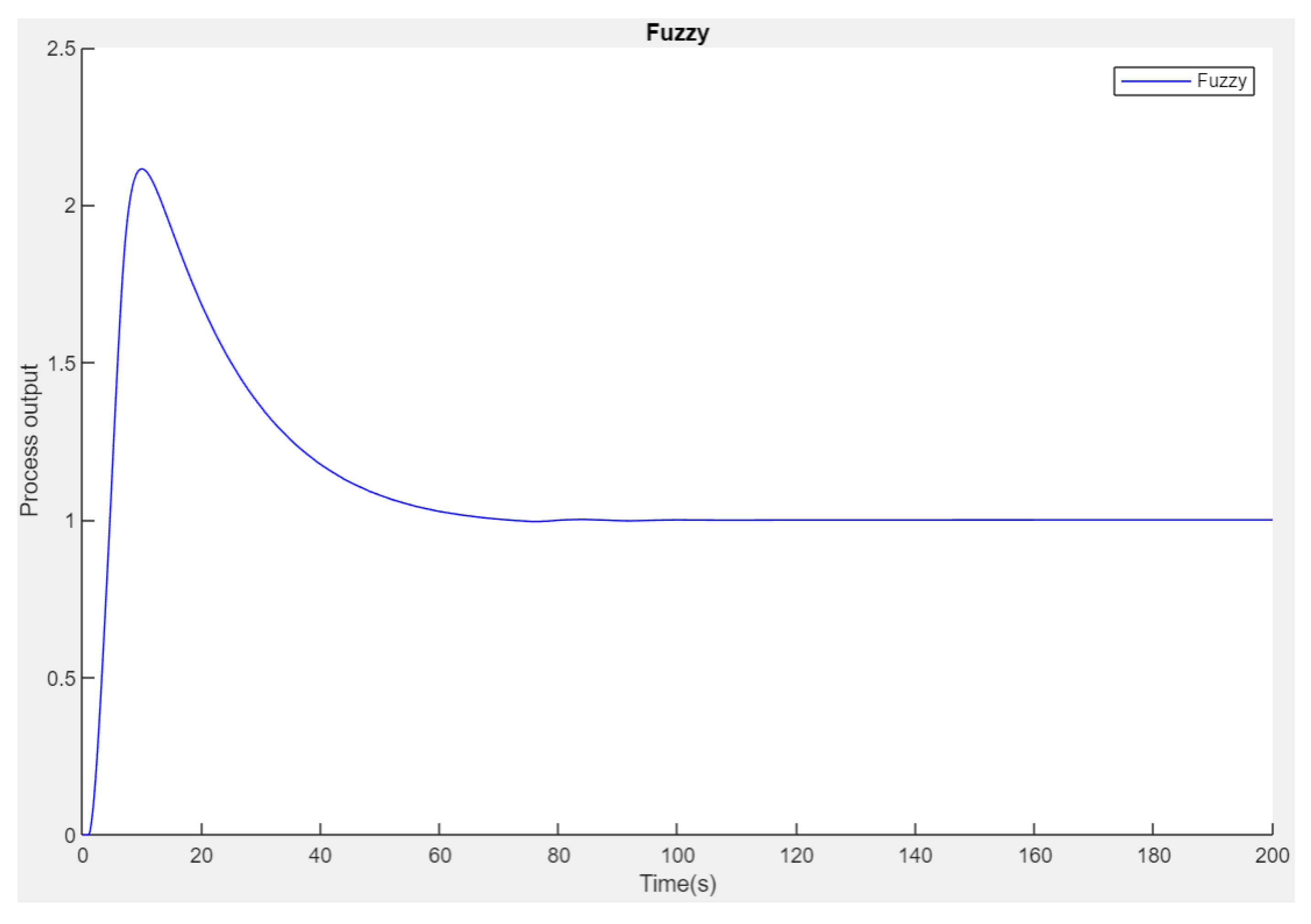
Figure 14.
Fuzzy, MPC and PID response.
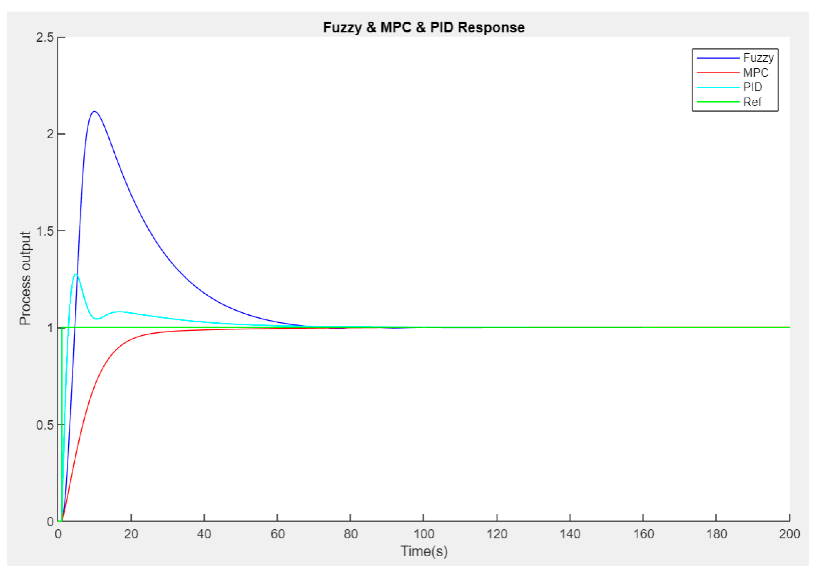
Figure 15.
Error plot of PID, MPC and FLC controller.
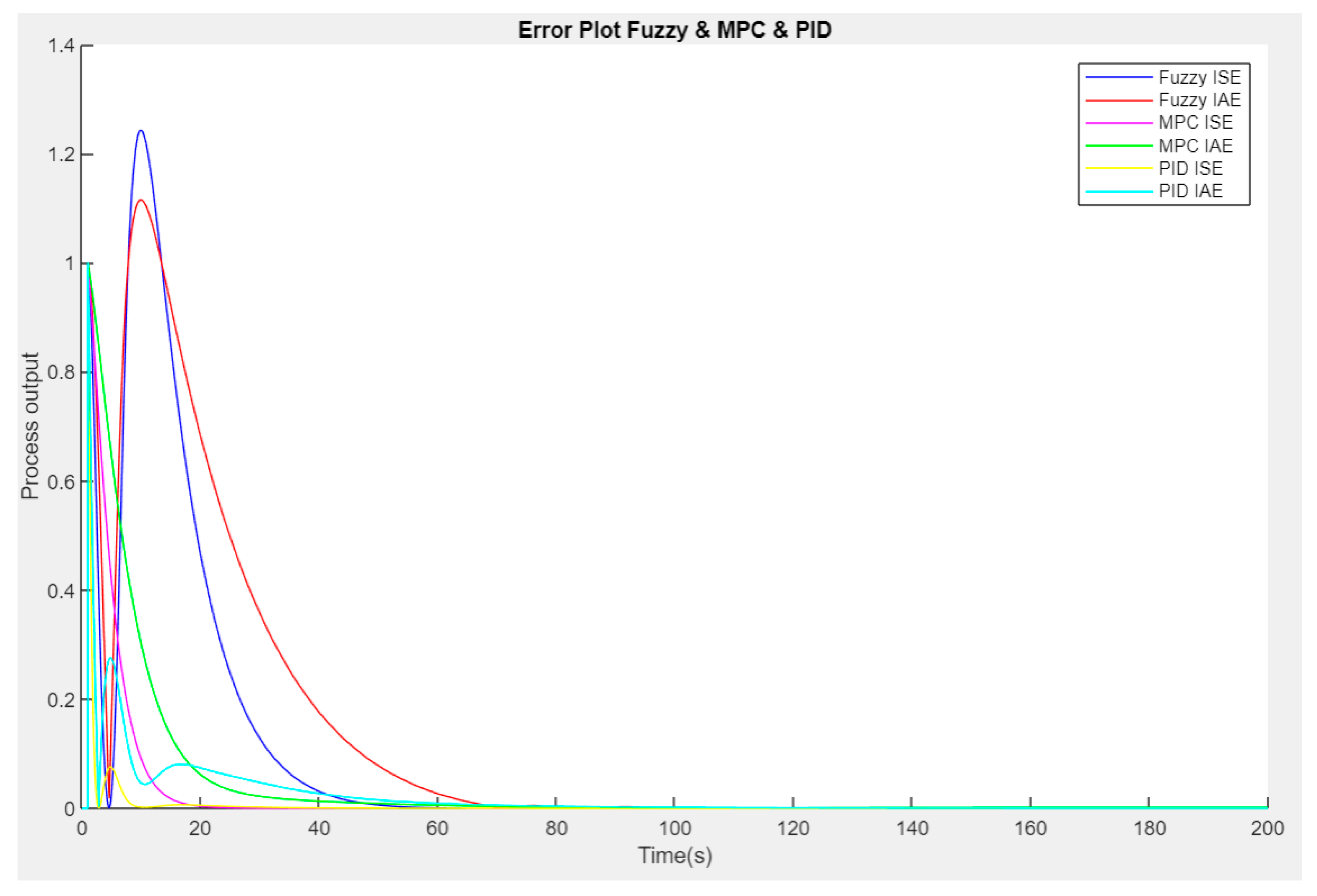

Table 1.
Sizing sheet of the heat exchanger.
| Fluid: | Unit of Measurement | Secondary Side | Primary Side | ||
|---|---|---|---|---|---|
| Density: | kg/m³ | 999.3 | 1,001.50 | ||
| Specific heat capacity: | kcal/(kg·°C) | 1.0032 | 1.0055 | ||
| Viscosity inlet: | cP | 1.17 | 1.67 | ||
| Viscosity outlet: | cP | 1.24 | 1.57 | ||
| Volume flow rate: | m³/h | 2.27 | 2.26 | ||
| Inlet temperature: | °C | 14 | 2 | ||
| Outlet temperature: | °C | 12 | 4 | ||
| Pressure drop: | mwg | 3.9 | 4 | ||
| Heat exchanged: | Mcal/h | 4.5 | |||
| Thermal conductivity: | kcal/(m·h·°C) | 0.509 | 0.4944 | ||
| LMTD: | K | 10 | |||
| Heat transfer coefficient: | kcal/(m²·h·°C) | 2,846 | |||
| Heat transfer area: | m² | 0.16 | |||
| Directions of the chilled water | Countercurrent | ||||
| Number of passes: | 1 | 1 | |||
| Effective margin: | % | 25 | |||
| Effective fouling resistance * 10000: | m²·h·C/kcal | 0.703 | |||
| Design pressure (MAWP): | at | 10.5 10.5 | |||
| Test pressure: | at | 13.7 13.7 | |||
| Design temperature max.: | °C | 65.6 65.6 | |||
| Design temperature min. (MDMT): | °C | -55.6 | |||
| Channel arrangement: | 1*3 L 1*3 L | ||||
| Pressure vessel approval: | ASME UM-stamp | ||||
| Number of plates: | 7 | ||||
| Nominal A-dimension: | mm | 26 | |||
| Extension capacity: | 18 plates | ||||
Table 2.
Control parameters.
| Control parameters of PID controller | Control parameters of MPC controller |
Control parameters of FLC controller | |
|---|---|---|---|
| Rise time | 1.3781 | 12.6123 | 2.4947 |
| Setting time | 45.1349 | 32.9513 | 61.4277 |
| Setting min | 0.9647 | 0.90375 | 0.90572 |
| Setting max | 1.2761 | 1.0017 | 2.1154 |
| Overshoot | 27.6015 | 0 | 111.5483 |
| Undershoot | 0 | 0 | 0 |
| Peak | 1.2761 | 1.0017 | 2.1154 |
| Peak time | 4.9344 | 200 | 9.8476 |
Disclaimer/Publisher’s Note: The statements, opinions and data contained in all publications are solely those of the individual author(s) and contributor(s) and not of MDPI and/or the editor(s). MDPI and/or the editor(s) disclaim responsibility for any injury to people or property resulting from any ideas, methods, instructions or products referred to in the content. |
© 2024 by the authors. Licensee MDPI, Basel, Switzerland. This article is an open access article distributed under the terms and conditions of the Creative Commons Attribution (CC BY) license (http://creativecommons.org/licenses/by/4.0/).
Copyright: This open access article is published under a Creative Commons CC BY 4.0 license, which permit the free download, distribution, and reuse, provided that the author and preprint are cited in any reuse.


