
Submitted:
18 November 2024
Posted:
19 November 2024
You are already at the latest version
Abstract
In this study, we develop an extremal principle governing the far-from-equilibrium evolution of a system composed of structureless particles, utilizing the stochastic generalization of the quantum hydrodynamic analogy with random curvature wrinkles due to the gravitational background noise (GBN). For a classical phase, where quantum correlations decay over distances shorter than the average inter-molecular separation, the far-from-equilibrium kinetic equation can be formulated as a Fokker-Planck equation. We derive the velocity vector in phase space that maximizes the dissipation of a function analogous to energy, termed stochastic free energy. In quasi-isothermal, far-from-equilibrium states without chemical reactions—where elastic molecular collisions dominate—the maximum SFED reduces to Sawada's principle of maximum free energy dissipation. However, in the presence of chemical reactions or significant thermal gradients, this principle is violated, as additional dissipative contributions emerge, linking the true maximum to stochastic free energy dissipation. The study also shows that Malkus and Veronis's principle of maximum heat transfer is a special case of the theory. Generally speaking. as systems strive for maximum SFED, they progress toward equilibrium by transitioning through increasingly ordered states, facilitating self-organization of matter. Nonetheless, the self-organization in fluids and gases is insufficient to form complex living structures, requiring a series of additional conditions such as the need of solid rheological properties, united to the need of information storing. The work highlights synergistic effects and efficiency-enhancing tendencies driving evolution, revealing new analogies between biological and social systems. Furthermore, it suggests that natural intelligence, as well as the consciousness, are inherent characteristics of the universe's physics, though certain side effects of the natural selection complicate the advancement toward efficiency and prosperity. The theory demonstrates that the ordering process is not continuous but experiences catastrophic events and collapses, which lead to the formation of new, more efficient systems. Finally, contemporary social behaviors are analyzed from the standpoint of the theory, including aspects such as monetary inflation control, economic expansion-recession cycles and the alternation between war and peace, providing insights on how to better address current challenges.
Keywords:
Determinism
; Probabilism
; Quantum to classic mechanics coexsistence
; Gravitational effects in quantum mechanics
; matter self-assembling
; Free will
1. Introduction
The challenge of establishing a solid physical basis for explaining the emergence of organized biological systems has troubled scientists for quite some time. A parallel situation emerged in the early 20th century within the realms of physics and chemistry. All scientists were of the belief that if they could discern the governing physical laws for each individual component of a chemical system, they could subsequently describe its properties as a function of these physical variables. While this notion was theoretically sound, it proved impractical in practice, as the theories of physical science remained incomplete to this task until the advent of quantum theory.
A similar predicament exists in the relationship between physics and biology. In theory, understanding the physical evolution of each constituent part of a biological system should enable us to describe any biological system. However, this aspiration encounters significant obstacles, not only due to the immense computational demands it entails but also because it conflicts with the established law of entropy increase. Many researchers share the conviction that this law is incomplete and a general principle exists.
The research on order generation and matter self-assembling in the field dates back to the 1930s [1,2,3,4,5,6,7,8]. Various extremal principles have been proposed for self-organized regimes governed by classical linear and non-linear non-equilibrium thermodynamic laws, with particular emphasis on stable stationary configurations.
However, a comprehensive understanding remains elusive. In 1945, Prigogine [1,2] introduced the "Theorem of Minimum Entropy Production," which applies exclusively to near-equilibrium stationary states. Prigogine's proof has faced substantial criticism [3]. Šilhavý [4] suggests that the extremal principle of near-equilibrium thermodynamics lacks a counterpart for far-from-equilibrium steady states, despite claims in the literature.
Sawada [5], in the context of Earth's atmospheric energy transport, proposed the principle of the largest entropy increment per unit time. He cited Malkus and Veronis's work in fluid mechanics [6], which demonstrated the principle of maximum heat current, as a particular example of maximum entropy production given certain assigned boundary conditions. However, this inference is not generally valid.
The concept of energy dissipation rate first appeared in Onsager's work [7] on this subject. Grandy [8] extensively discussed potential principles related to extremal entropy production and/or energy dissipation rates. He pointed out the challenge of defining the rate of internal entropy production in general cases, suggesting that, for predicting the course of a process, the extremum of the rate of energy dissipation may be more useful than that of entropy production.
Sawada and Suzuki [9] confirmed, through numerical simulations and experiments, the maximum rate of energy dissipation in electro-convective instabilities. To this day, the debate continues regarding the principle of maximum free energy dissipation (MFED) and Prigogine's principle.
An alternative approach to understanding far-from-equilibrium evolution can be formulated using Langevin equations, which describe dynamics at a coarse-grained scale in some cases. Langevin equations can be derived using various techniques, such as the Poisson transformation [10] and Fock space formalism [11]. Exact formulations exist occasionally for non-linear reaction kinetics and a few other problems. In some cases, a Langevin equation can be assumed from a phenomenological standpoint, where the approximate dynamics are decided a priori. However, achieving a rigorous Langevin description in this context is challenging.
The way out is to derive satisfactory Langevin equations from a microscopic model. In this work, we employ the stochastic generalization of the Madelung’s quantum hydrodynamic analogy [12,13,14,15] as microscopic model from which to derive the classical non-equilibrium kinetics emerging at the coarse-grained macro-scale.
Prigogine's work is not applicable under conditions far from equilibrium because it derives the system's entropy production through a series expansion, which is essentially a semi-empirical approach with a limited range of convergence and lacking connections to microscopic physical variables rooted in quantum physics. Consequently, the limitations of Prigogine's theory stem from its classical foundations.
Conversely, a more fundamental approach could, in principle, be adopted by treating any far-from-equilibrium system as a quantum system. In this case, the evolution of the system's wavefunction would also need to account for its incoherent dynamics, leading to irreversible phenomena on a macroscopic scale. Although complex, if we can employ the quantum model to derive a coarse-grained macroscopic description, a more fundamental criterion for the system's spontaneous progression should naturally emerge. The limitation of this approach lies in the fact that the connection between quantum mechanics and classical mechanics remains unclear and is the subject of ongoing, intense, and contentious debate. [16,17,18,19,20,21,22,23,24,25,26,27,28,29,30,31].
To address this theoretical gap, there are various interpretations of quantum mechanics available, such as the many-worlds interpretation [16], Bohmian mechanics [17,18], modal interpretation [19], relational interpretation [20], consistent histories [21], transactional interpretation [22,23], QBism [24], Objective collapse theories [25], Madelung quantum hydrodynamics [26], and decoherence approach [27].
The decoherence approach explores the idea of achieving the statistical mixture by means of the loss of quantum coherence caused by the presence of the environment. Decoherence is observed to occur within the system by considering it as a sub-part of larger quantum system, with its interaction being semi-empirically defined through non-unitary interactions [27].
The proposed solution for the evolution of irreversible systems is achieved through a local quantum pseudo-diffusional effect [28], where the system is embedded in a vastly large environment. This behavior, driven by quantum diffusion, but with a non-definite positive diffusion coefficient, implies a recurrence time—a period after which the entire system returns to its initial state [29] with an anti-entropic evolution. However, the success of decoherence theory depends on the exceedingly long duration of this recurrence time.
Furthermore, the quantum pseudo-diffusional effect requires that simultaneous anti-entropic changes occur in other regions of the overall quantum system before the recurrence time elapses. This issue is addressed by assuming an infinite environment, thereby making the probability of these anti-entropic effects occurring within the local system approach zero. The major objections to this view are that such spontaneous anti-entropic phenomena have not been observed anywhere in the universe, and the assumption of distinguishability between the system and its environment subtly reintroduces the condition that the global system is classical.
The role of environmental fluctuations in quantum decoherence is also confirmed through experimental and numerical simulations, which provide strong evidence that decoherence and the localization of quantum states result from interactions with stochastic and gravitational fluctuations [30,31,32,33,34].
The quantum-to-classical transition, the role of the observer, the existence of pre-measurement reality, and the self-sustained classical state of the global system are long-standing, fundamental unresolved issues in modern physics [35,36,37,38,39,40] the EPR paradox, von Neumann theorem, and related works]. Nevertheless, some approaches, such as Bohm's non-local hidden variable theory and Objective Collapse models, have introduced new insights, advancing scientific thought. Recently, by incorporating the effect of the gravitational background—considered as spatiotemporal curvature fluctuations—into Madelung quantum hydrodynamics, the author has proposed a stochastic hydrodynamic theory [41] that potentially resolves quantum paradoxes and reconciles relativistic locality with quantum non-locality. The gravitational stochastic background, stemming from relics of the Big Bang and the general relativistic dynamics of bodies, causes the reference system to become interconnected with the dynamics of bodies. This noise acts as an external system or thermostat, though it is not truly external to the system. From this perspective, the universal quantum system is self-fluctuating, and on a scale larger than the de Broglie wavelength, it gradually loses quantum coherence, giving rise to classical mechanics.
The Madelung approach, a specific case of the Bohm mechanics [39], has the important characteristic of being both mathematically equivalent to the Schrödinger approach [12,13.26] and treating the evolution of the wave function in a classical-like way, as the motion of a mass density governed by the impulse .
The Madelung description offers the advantage of a controlled transition to classical mechanics when the so-called quantum pseudo-potential tends to zero [40]. However, manually removing the quantum potential from the quantum hydrodynamic equations to derive classical mechanics is mathematically unjustified and invalid, as it effectively eliminates stationary quantum eigenstates and significantly alters the mathematical structure of the equations of motion. Therefore, to account for the effect of the quantum potential in the presence of random fluctuations and bridge the gap between the quantum non-local and classical descriptions, a more rigorous and analytical approach within the hydrodynamic framework is required [40].
The Stochastic Quantum Hydrodynamics Model (SQHM) explains the emergence of a large-scale classical state as resulting from the loss of quantum entanglement, due to the shielding of the quantum potential at the wavefunction tails by noise fluctuations. This effect causes global wavefunction decay (collapse) and quantum decoherence in systems whose components are separated by exceedingly large distances, leading to statistical mixing and classical behavior. From this perspective, the SQHM aligns with Objective Collapse Theories. The unique feature of SQHM is that it focuses on the strength of the quantum potential, originating from wavefunction tails, as the key factor determining whether a macroscopically large system is in a classical state, rather than its infinitesimal mass density.
This formulation aligns with recent studies that explore the transition from quantum to classical dynamics by incorporating stochastic elements into the quantum hydrodynamic framework [41]
The stochastic extension of the Madelung quantum hydrodynamic equations can provide an analytical unitary description from microscopic quantum dynamics to macroscopic behavior. As a result, it offers a way to explore the quantum foundations of irreversibility in far-from-equilibrium conditions and may lead to the formulation of a broader physical principle governing the emergence of spontaneous order and self-assembly of matter
2. The Quantum Stochastic Hydrodynamic Model
The Madelung quantum hydrodynamic representation transforms the Schrodinger equation [12,13,26]
for the complex wave function , into two equations of real variable: the conservation equation for the mass density
and the motion equation for the momentum ,
whereand where
Following the scientific hypothesis that considers the gravitational background noise (GBN) as a source of quantum decoherence [42], first proposed in the Calogero conjecture [43] and by introducing it into Madelung quantum hydrodynamics, equation (1.4) yields a generalized stochastic quantum model capable of describing wavefunction collapse dynamics and the measurement process, leading to a fully self-consistent quantum theory.
The fluctuating energy content of GBN leads to local variations in equivalent mass density. As shown in [40], the SQHM is defined by the following assumptions:
- The additional mass density generated by GBN is described by the wavefunction with density ;
- The associated energy density of GBN is proportional to ;
- The additional mass is defined by the identity
- The additional mass is assumed to not interact with the mass of the physical system (since the gravitational interaction is sufficiently weak to be disregarded).
- Under this assumption, the wavefunction of the overall system reads as
Additionally, given that the energy density of GBN is quite small, the mass density is presumed to be significantly smaller than the body mass density typically encountered in physical problems. Hence, considering the mass to be much smaller than the mass of the system, in Equations (3) and (4) we can assume . Thence, by introducing the mass density fluctuations, through , into the quantum potential (4), following the procedure given in reference [40], it is possible for the complex field
to obtain the quantum-stochastic hydrodynamic equations of evolution that, for systems whose physical length is of order of the De Broglie length, reads
Given the physical length of the system, the diffusion coefficient in (7) can be readjusted as
where is a positive pure number, depending by the characteristics of the system [40], and
is the De Broglie length defining physical distance below which the quantum coherence is maintained in presence of fluctuations since for or the Madelung quantum deterministic limit is recovered.
In fact, given the semiempirical parameter defined by the identity [40 and references therein]
expressing the ability of the system to dissipate energy, it is possible to show [40] that
and therefore that the conventional quantum mechanics in the form of the quantum hydrodynamic representation (1-4) is recovered for noise amplitude tending to zero or equivalently for microscopic systems whose physical length is much smaller than the De Broglie length.
In the quantum-stochastic hydrodynamic representation, is the probability mass density (PMD) determined by the probability transition function [44] obeying to the Smoluchowski conservation equation [44] for the Marcovian process (7)
establishing the phase-space mass density conservation
that leads to the mass density distribution in the spacetime
In the context of (7-9), does not denote the quantum wavefunction; rather, it represents the generalized quantum-stochastic probability wave. that adheres to the limit.
It is worth noting that the SQHM equations (7-9), stemming from the presence of noise curvature wrinkles of spacetime (a form of dark energy) both of relic origin from big bang and from bodies dynamics in curved spacetime, describe a self-fluctuating quantum system where the noise is an intrinsic property of the reference system that is not generated by an environment. An in-depth discussion regarding the property of true randomness or pseudo-randomness of the gravitational background noise is provided in section 3.1.1. .
2.1. Emerging Classical Mechanics on Large Size Systems
When manually nullifying the quantum potential in the equations of motion for quantum hydrodynamics (1-3), the classical equation of motion emerges [13]. However, despite the apparent validity of this claim, such an operation is not mathematically sound as it alters the essential characteristics of the quantum hydrodynamic equations. Specifically, this action leads to the elimination of stationary configurations, i.e., quantum eigenstates, as the balancing force of the quantum potential against the Hamiltonian force [24]—which establishes their stationary condition—is eliminated. Consequently, even a small quantum potential cannot be disregarded in conventional quantum mechanics representing the zero-noise 'deterministic' limit of the quantum-stochastic hydrodynamic model (7-9)."
Conversely, in the stochastic generalization, it is possible to correctly neglect the quantum potential in (7) when its force is much smaller than the force noise such as, by (7), that leads to condition
and hence, in a coarse-grained description with elemental cell side , such as
where is the physical length of the system.
It is worth noting that, despite the noise having a zero mean, the mean of the fluctuations in the quantum potential, denoted as , is not null. This not-null mean contributes to the frictional dissipative force in equation (7). Consequently, the stochastic sequence of noise inputs disrupts the coherent dynamic evolution of the quantum superposition of states, leading them to decay to a stationary mass density distribution with . Moreover, by observing that the stochastic force noise
grows with the size of the system, for macroscopic systems (i.e., ), condition (17) can be satisfied if
In order to achieve a large-scale description completely free from non-local quantum potential interaction, a more stringent requirement can be imposed, such as
Recognizing that since for linear systems it holds
we readily can observe that these systems are incapable of generating macroscopic classical phases. Generally speaking, as the Hamiltonian potential strengthens, the wave function localization increases, and the quantum potential behavior at infinity becomes more prominent.
In fact, by considering the mass density
where is polynomial of order k, it becomes evident that a vanishing quantum potential interaction at infinity is achieved for .
On the other hand, for instance, for gas phases with particles that interact by the Lennard-Jones potential, whose long-distance wave function reads [45]
leading to the quantum potential
developing the quantum force
in a sufficiently rarefied phase, can lead to large-scale classical behavior [40]
It is interesting to note that in (25), the quantum potential coincides with the hard sphere potential of the “pseudo potential Hamiltonian model” of the Gross-Pitaevskii equation [46,47], where is the boson-boson s-wave scattering length.
By observing that, to fulfill condition (21), we can sufficiently require that
so that it is possible to define the quantum potential range of interaction as [40]
Relation (28) provides a measure of the range of interaction associated with quantum non-local potential.
It is worth noting that the quantum non-local interaction extends up to a distance on the order of the largest length between and .. Below , a weak quantum potential emerges due to the damping of the noise. However, above and below , the quantum potential is strong enough not to be shielded by fluctuations, leading to the emergence of quantum behavior.
Therefore, quantum non-local effects can be extended by increasing as a result of lowering the temperature or by strengthening the Hamiltonian potential, which leads to larger values of . In the latter case, for instance, larger values of can be achieved by extending the linear range of Hamiltonian interaction between particles
For instance, when examining phenomena at intermolecular distances where the interaction is modeled as linear, the behavior exhibits quantum characteristics (e.g., X-ray diffraction from a crystalline lattice). However, when observing macroscopic behaviors, such as elastic sound waves, which primarily depend by the non-linear part of the Lennard-Jones interatomic potential without affecting the linear part, classical behavior emerges.
2.2. The Lindemann Constant at the Melting Point of Quantum Lattice
A validation test for the SQHM can be conducted by comparing its theoretical predictions with experimental data on the transition from a quantum solid lattice to a classical amorphous fluid. Specifically, we show that the SQHM can theoretically derive the Lindemann constant at the melting point of a solid lattice, representing the quantum-to-classical transition threshold, something that has remained unexplained within the frameworks of both conventional quantum and classical theories.
For a system of Lennard-Jones interacting particles, the quantum potential range of interaction reads
where (with ) represents the distance up to which the interatomic force is approximately linear, and denotes the atomic equilibrium distance.
The physical significance of the quantum potential length of interaction is evident during the quantum-to-classical transition in a crystalline solid at its melting point.
Assuming that, to preserve quantum coherence within the quantum lattice, the atomic wave function (around the equilibrium distance) extends over a distance smaller than the quantum coherence length, the square root of its variance must result smaller than which corresponds to the melting point.
Based on these assumptions, the Lindemann constant defined as [44]
can be expressed as and it can be theoretically calculated, as
that, being typically and , leads to
2.3. The Fluid-Superfluid Transition
If the Lindemann constant is derived from a quantum-to-classical transition governed by the strength of the Hamiltonian interaction, which determines the quantum potential interaction length, another validation of the SQHM can be obtained by its predictions on transitions induced by the change of De Broglie physical length such as the fluid-to-superfluid transition.
Given that the De Broglie distance is temperature-dependent, it impacts on the fluid-superfluid transition in monomolecular liquids at extremely low temperatures, when it equals the mean molecular distance as observed in . The approach to this scenario is elaborated in reference [48,49], where, for the - interaction, the potential well is assumed to be.
In this context, represents the Lennard-Jones potential depth, denotes the mean - inter-atomic distance where .
As the superfluid transition temperature is attained, the De Broglie length overlaps more and more the -wavefunctions within the potential depth. Therefore, we observe the gradual increase of superfluid concentration within the interval
Therefore, the total superfluid occurs as soon as the De Broglie length covers all the - potential well for .
However, for , we have no superfluid . Therefore, given that
when , the superfluid-to-normal density ratio of 50% is reached at the temperature
where the mass is assumed to be , in good agreement with the experimental data measured in reference [50].
On the other hand, given that for , all pairs of enter the quantum state, the superfluid ratio of 100% is attained at the temperature
also consistent with the experimental data from reference [50], which is approximately .
Moreover, by employing the superfluid ratio of 38% at the -point of, such that , the transition temperature is determined to be
in good agreement with the measured superfluid transition temperature of .
It is worth noting that there are two ways to establish quantum macroscopic behavior. One approach involves lowering the temperature, effectively increasing the de Broglie length. The second approach is to strength the Hamiltonian interaction, among the particles, to enhance the quantum potential length of interaction. The latter effect can be achieved simply by increasing the distance over which the Hamiltonian interaction remains linear. In the forme case the De Broglie length induces a strong and macroscopic quantum behavior, while in the latter one, induce by the quantum potential range of interaction, the quantum behavior is weaker and is limited to the electron delocalization bringing to the normal metal conductivity.
From this standpoint, we can conceptualize the classical mechanics as emergent from a decoherent outcome of quantum mechanics when fluctuating spacetime reference background is involved.
It is also important to highlight that the limited strength of the Hamiltonian interaction over long distances is the key factor allowing classical behavior to manifest.
Moreover, by observing that systems featuring interactions that are weaker than linear interactions are classically chaotic, it follows that the classical cahoticity is widespread characteristic of the classical reality.
To this respect, the strong divergence of chaotic trajectories of motion due to high Lyapunov exponents also contributes to facilitate the destruction of the quantum coherence maintained by the quantum potential by leading to high values of the dissipation parameter in (12).
2.4. Measurement Process and the Finite Range of Nonlocal Quantum Potential Interactions
Throughout the course of measurement, there exists the possibility of a conventional quantum interaction between the sensing component within the experimental setup and the system under examination. This interaction concludes when the measuring apparatus is relocated to a considerable distance from the system. Within the SQHM framework, this relocation is imperative and must surpass specified distances and.
Following this relocation, the measuring apparatus manages the "interaction output." This typically involves a classical, irreversible process, characterized by the time arrow, leading to the determination of the macroscopic measurement result.
Consequently, the phenomenon of decoherence assumes a pivotal role in the measurement process. Decoherence facilitates the establishment of a large-scale classical framework, ensuring authentic quantum isolation between the measuring apparatus and the system, both pre and post the measurement event.
This quantum-isolated state, both at the initial and final stages, holds paramount significance in determining the temporal duration of the measurement and in collecting statistical data through a series of independent repeated measurements.
It is crucial to underscore that, within the confines of the SQHM, merely relocating the measured system to an infinite distance before and after the measurement, as commonly practiced, falls short in guaranteeing the independence of the system and the measuring apparatus if either or is met. Therefore, the existence of a macroscopic classical reality remains indispensable for the execution of the measure process in quantum mechanics.
2.5. Minimum Measurement Uncertainty in Fluctuating Spacetime Background
Any quantum theory aiming to elucidate the evolution of a physical system across various scales, at any order of magnitude, must inherently address the transition from quantum mechanical properties to the emergent classical behavior observed at larger magnitudes. The fundamental disparities between the two descriptions are encapsulated by the minimum uncertainty principle in quantum mechanics, signifying the inherent incompatibility of concurrently measuring conjugated variables, and the finite speed of propagation of interactions and information in local classical relativistic mechanics.
Should a system fully adhere to the "deterministic" conventions of quantum mechanics up to a distance, possibly smaller than, where its subparts lack individual identities, the independent observer, to gain information about the system, needs to maintain a separation distance bigger than both before and after the process.
Should a system fully adhere to the conventional quantum mechanics within a physical length, smaller than , where its subparts lack individual identities, the independent observer, that wants to gain information about the system, needs to maintain a separation distance bigger than both before and after the process.
Therefore, due to the finite speed of propagation of interactions and information, the process cannot be executed in a time frame shorter than
Furthermore, considering the Gaussian noise in (7) with the diffusion coefficient proportional to, we find that the mean value of energy fluctuation is for the degree of freedom. As a result, a nonrelativistic ( ) scalar structureless particle, with mass m, exhibits an energy variance of
from which it follows that
It is noteworthy that the product remains constant, as the increase in energy variance with the square root of precisely offsets the corresponding decrease in the minimum acquisition time . This outcome holds true when establishing the uncertainty relations between the position and momentum of a particle with mass m.
If we acquire information about the spatial position of a particle with precision , we effectively exclude the space beyond this distance from the quantum non-local interaction of the particle, and consequently
the variance of its relativistic momentum due to the fluctuations reads
and the uncertainty relation reads
Equating (62) to the uncertainty value, such as
or
It follows that represents the physical length below which quantum entanglement is fully effective, and it signifies the deterministic limit of the SQHM, specifically the realization of quantum mechanics.
As far as it concerns the theoretical minimum uncertainty of quantum mechanics, obtainable from the minimum indeterminacy (59, 62) in the limit of quantum mechanics (and) in the non-relativistic limit (), we have that
With regard to the minimum uncertainty of quantum mechanics, attainable from the minimum indeterminacy (59, 62) in the limit of (), in the non-relativistic limit (), it follows that
and therefore that
That constitutes the minimum uncertainty in quantum mechanics, obtained as the deterministic limit of the SQHM.
It's worth noting that, owing to the finite speed of light, the SQHM extends the uncertainty relations to all conjugate variables of 4D spacetime. In conventional quantum mechanics, deriving the energy-time uncertainty is not possible because the time operator is not defined.
Furthermore, it is interesting to note that in the relativistic limit of quantum mechanics (and), influenced by the finite speed of light, the minimum acquisition time of information in the quantum limit is expressed as follows
The result (71) indicates that performing a measurement in a fully deterministic quantum mechanical global system is not feasible, as its duration would be infinite.
Given that non-locality is restricted to domains with physical lengths on the order of , and information about a quantum system cannot be transmitted faster than the speed of light (violating the uncertainty principle otherwise), local realism is established within the coarse-grained macroscopic physics where domains of order of reduce to a point.
The paradox of "spooky action at a distance" is confined to microscopic distances (smaller than ), where quantum mechanics is described in the low-velocity limit, assuming and . This leads to the apparent instantaneous transmission of interaction over a distance.
It is also noteworthy that in the presence of noise, the measure indeterminacy has a relativistic correction since leading to the minimum uncertainty in a quantum system submitted to gravitational background noise ()
It is also noteworthy that in the presence of noise, the measured indeterminacy undergoes a relativistic correction, as expressed by , resulting in the minimum uncertainty in a quantum system subject to gravitational background noise ():
and
This can become significant for light particles (with ), but in quantum mechanics, at , the uncertainty relations remain unchanged.
2.6. The Discrete Nature of Spacetime
Within the framework of the SQHM, incorporating the uncertainty on measure in fluctuating quantum system and the maximum attainable velocity of the speed of light such as
it follows that the uncertainty relations
leads to and, consequently, to
where is the Compton’s length.
Identity (76) reveals that the maximum concentration of the mass of a body, compatible with the uncertainty principle, is within an elemental volume with a side length equal to half of its Compton wavelength.
This result holds significant implications for black hole (BH) formation. To form a BH, all the mass must be compressed within a sphere of the gravitational radiusthat cannot have a radius smaller than the Compton length , giving rise to the relationship:
which further leads to the condition:
indicating that the BH mass
where .
This in a vacuum at zero background temperature, If we consider positive temperature as in (57) it follows that
leading to
and, consequently, to
which leads to the condition that for a BH reads
Result (67) shows that, in the presence of a positive temperature greater than zero, a black hole with Planck mass becomes unstable, requiring additional mass to achieve stability. It is worth noting that this temperature-driven instability could be the mechanism that destabilized pre-big bang black hole [51], potentially leading to its extrusion beyond the gravitational radius and triggering the big bang.
Result (60) demonstrates that the maximum mass density, constrained by quantum laws—specifically the minimum uncertainty principle—is attained when confined within a sphere whose diameter equals half the Compton wavelength. This implies that,in this case, the repulsive quantum potential becomes infinite and insurmountable. Consequently, within the gravitational radius, the black hole's mass cannot collapse into a singular point; rather, the collapse is halted by quantum forces before reaching a sphere with a radius equal to the Compton wavelength. In equilibrium, the gravitational force and the quantum potential exactly counteract each other.
Considering the hypothesis that spacetime has a discrete structure, it follows that, given the nature of an elemental volume of spacetime—defined as the volume within which mass density is uniformly distributed—the assumption that the Planck length represents the smallest discrete elemental volume is unsustainable. This would make it impossible to compress the mass of large black holes, with masses greater than , within a sphere whose diameter is half the Compton wavelength, thereby preventing the attainment of gravitational equilibrium [52,53]. This suggests that such a discrete description of the universe is incompatible with the gravitational dynamics of black holes.
On the other hand, since existing black holes compress their mass into a core smaller than the Planck length [52,53], spacetime discretization would require elemental cells of even smaller volumes. In the analogy of a simulation, the maximum grid density is defined by the size of these elemental cells of spacetime.
Thus, it is important to consider that the assumption that the smallest discrete spacetime distance corresponds to the minimum possible Compton wavelength
—derived from the maximum possible mass/energy density, which is the mass/energy of the universe—provides a criterion to rationalize the universe's mass. This helps explain why the mass of the universe is not higher than its observed value, as it is intrinsically tied to the minimum length of the discrete spacetime element. If the pre-big-bang black hole was generated by an anomalous fluctuation gravitationally confined within an elemental cell of spacetime, its mass content could not be smaller than that of the universe.
2.6.1. Dynamics of Wavefunction Collapse
The Markov process (7) in the limit of slow kinetics (see Equation (74) below) can be described by the Smolukowski equation for the Markov probability transition function (PTF) [44]
where the PTF is the probability that in time interval τ is transferred to point q.
The conservation of the PMD shows that the PTF displaces the PMD according to the rule [44]
Generally, for the quantum case, Equation (68) cannot be reduced to a Fokker–Planck equation (FPE). The functional dependence of by , and by the PTF , produces non-Gaussian terms [40].
Nonetheless, if, at initial time, is stationary (e.g., quantum eigenstate) close to the long-time final stationary distribution , it is possible to assume that the quantum potential is about constant in time as a Hamilton potential following the approximation
Being in this case the quantum potential independent by the mass density time evolution, the stationary long-time solutions can be approximately described by the Fokker–Planck equation
where
leading to the final equilibrium of the stationary quantum configuration
In ref. [40] the stationary states of a harmonic oscillator obeying (72) are shown. The results show that the quantum eigenstates are stable and maintain their shape (with a small change in their variance) when subject to fluctuations.
2.6.2. Evolution of the PMD of Superposition of States Submitted to Stochastic Noise
The quantum evolution of not-stationary state superpositions (not considering fast kinetics and/or jumps (eventually due to external inputs)) involves the integration of Equation (7) in the form
in which fast variables are eliminated.
By utilizing both the Smolukowski Equation (68) and the associated conservation Equation (69) for the PMD , it is possible to integrate (74) by using its second-order discrete expansion
where
where has a Gaussian zero mean and unitary variance which probability function , for , reads as
where the midpoint approximation has been introduced and where
and
are the solutions of the deterministic problem:
As shown in ref. [40], the PTF can be achieved after successive steps of approximation and reads
and the PMD at the -th instant reads
leading to the velocity field
Moreover, the continuous limit of the PTF gives
where.
2.6.3. General Features of Relaxation of Quantum Superposition of States
The classical Brownian process admits the stationary long-time solution
where, leading to solution [58]
As far as it concerns in (86) it cannot be expressed in a closed form, unlike (87), because it is contingent on the particular relaxation path the system follows toward the steady state. This path is significantly influenced by the initial conditions, namely the MDD as well as , and, consequently, by the initial time at which the quantum superposition of states is subjected to fluctuations. This means that the output of a measure to an eigenstate depends by the initial instant at which the system plus the measure system perform the measure. Therefore, if we repeat the measure statistically we end with a different output.
In addition, from (75), we can see that depends on the exact sequence of inputs of stochastic noise. This fact becomes more critical in classically chaotic systems since very small differences can lead to relevant divergences of the trajectories in a short time. Therefore, in principle, different stationary configurations (analogues of quantum eigenstates) can be reached whenever starting from identical superposition of states. Therefore, in classically chaotic systems, Born’s rule can also be applied to the measurement of a single quantum state.
Even if , it is worth noting that, to have finite quantum lengths and , necessary to have the quantum-decoupled classical environment (or measuring apparatus), also the nonlinearity of the overall system (system–environment) is necessary.
Quantum decoherence, which leads to the decay of superposition states, is significantly enhanced by the pervasive classical chaotic behavior observed in real systems. In contrast, a perfectly linear universal system would preserve quantum correlations on a global scale and would never allow quantum decoupling between the system and the experimental apparatus performing the measurement. It is important to note that even the decoupling of the system from the environment would be impossible, as quantum systems function as an integrated whole. Therefore, simply assuming the existence of separate systems and environments subtly introduces a classical condition into the nature of the overall supersystem.
Furthermore, since equation (7) is valid only in the leading order approximation of (i.e., during a slow relaxation process with small amplitude fluctuations) [40], in cases of large fluctuations occurring over a timescale much longer than the relaxation period of , transitions may occur to configurations not captured by (86), potentially leading from a stationary eigenstate to a new superposition of states. In this case, relaxation will once again proceed toward another stationary state. The given by (84) describes the relaxation process occurring during the time interval between two large fluctuations, rather than the system’s evolution toward a statistical mixture. Due to the extended timescales associated with these jumping processes, a system consisting of a significant number of particles (independent subsystems) undergoes gradual relaxation towards a statistical mixture. The statistical distribution of this mixture is determined by the temperature-dependent behavior of the diffusion coefficient.
2.7. EPR Paradox and Pre-Existing Reality in the SQHM
The SQHM (Stochastic Quantum Hamiltonian Mechanics) emphasizes that, despite the well-defined, reversible, and deterministic framework of quantum theory, its foundation remains incomplete. In particular, SQHM highlights that the measurement process is not accounted for within the deterministic "Hamiltonian" framework of standard quantum mechanics. Instead, it is better understood as a phenomenon described by a quantum stochastic approach.
SQHM reveals that standard quantum mechanics is essentially the deterministic, "zero-noise" limit of a broader quantum-stochastic theory, which arises from fluctuations in the spacetime gravitational background. In this context, zero-noise quantum mechanics defines the deterministic evolution of the system's "probabilistic wave." However, SQHM suggests that the term "probabilistic wave" is somewhat misleading, as it reflects the probabilistic nature of the measurement process—something standard quantum mechanics cannot fully explain. Since SQHM provides a framework that accounts for both wavefunction collapse and the measurement process, it proposes "state wave" as a more accurate term.
Moreover, SQHM reinstates the principle of determinism into quantum theory by clarifying that quantum mechanics describes the deterministic evolution of the system's "state wave." The apparent probabilistic outcomes arise from the influence of fluctuating gravitational backgrounds. SQHM also addresses the long-standing question of whether reality exists prior to measurement. While the Copenhagen interpretation suggests that reality only emerges when a measurement forces the system into a stable eigenstate, SQHM proposes that the world naturally self-decays through macroscopic-scale decoherence. In this view, only stable macroscopic eigenstates persist, establishing a lasting reality that exists even before measurement occurs.
With regard to the EPR paradox, SQHM shows that, in a perfectly deterministic (coherent) quantum universe, it is impossible to fully decouple the measuring apparatus from the system and therefore it is impossible to realize a measure within a finite time interval. Such decoupling can only be achieved in a large-scale classical supersystem—a quantum system embedded in 4D spacetime with a fluctuating background. In this scenario, quantum entanglement, driven by quantum potential, extends only over a finite distance. Thus, SQHM restores local relativistic causality in presence of GBN on macroscopic reality.
If the Lennard-Jones interparticle potential produces a sufficiently weak force, leading to a microscopic range of quantum non-local interactions and a large-scale classical phase, photons, as shown in reference [40], retain their quantum properties at the macroscopic level due to their infinite quantum potential range of action. As a result, photons are the ideal particles for experiments designed to demonstrate the features of quantum entanglement over long distances.
In order to clearly describe the standpoint of the SQHM on this argument, we can analyze the output of two entangled photon experiments traveling in opposite directions in the state
where and are vertical and horizontal polarizations, respectively, and is a constant phase coefficient.
Photons “one” and “two” impact polarizers (Alice) and (Bob) with polarization axes positioned at angles and relative to the horizontal axis, respectively. For our purpose, we can assume .
The probability that photon “two” also passes through Bob’s polarizer is .
As widely held by the majority of the scientific community in quantum mechanics physics, when photon “one” passes through polarizer with its axes at an angle of , the state of photon “two” instantaneously collapses to a linear polarized state at the same angle , resulting in the combined state .
In the context of the SQHM, able to describe the kinetics of the wavefunction collapse, the collapse is not instantaneous, and following the Copenhagen quantum mechanics standpoint, it needs to assert rigorously that the state of photon “two” is not defined before its measurement at the polarizer .
Therefore, after photon “one” passes through polarizer , from the standpoint of SQHM, we have to assume that the combined state is , where the state represents the state of photon “two” in the interaction with the residual quantum potential field generated by photon “one” at polarizer . The spatial extension of the field of the photon two, in the case the photons travel in opposite direction, is the double of that one crossed by the photon one before its adsorption. In this regard, it is noteworthy that the quantum potential is not proportional to the intensity of the field. Instead, it is proportional to its second derivative. Therefore, a minor perturbation in the field with a high frequency at the tail of photon two (during the absorption of photon one) can give rise to a significant quantum potential field .
When the residual part of the two entangled photons also passes through Bob’s polarizer, it makes the transition with probability . The duration of the photon two adsorption (wavefunction decay and measurement) due to its spatial extension, and finite light speed, it is just the time necessary to transfer the information about the measure of photon one to the place of photon two measurement. A possible experiment is proposed in ref. [4019].
Summarizing, the SQHM reveals the following key points:
- i.
- The SQHM posits that quantum mechanics represents the deterministic limit of a broader quantum stochastic theory;
- ii.
- Classical reality emerges at the macroscopic level, persisting as a preexisting reality before measurement;
- iii.
- The measurement process is feasible in a classical macroscopic world, because we can have really quantum decoupled and independent systems, namely the system and the measuring apparatus;
- iv.
- Determinism is acknowledged within standard quantum mechanics under the condition of zero GBN;.
- v.
- Locality is achieved at the macroscopic scale, where quantum non-local domains condense to punctual domains.
- vi.
- Determinism is recovered in quantum mechanics representing the zero-noise limit of the SQHM. The probabilistic nature of quantum measurement is introduced by the GBN.
- vii.
- The maximum light speed of the propagation of information and the local relativistic causality align with quantum uncertainty;
- viii.
- The SQHM addresses the GBN as playing the role of the hidden variable in the Bohm non-local hidden variable theory: The Bohm theory ascribes the indeterminacy of the measurement process to the unpredictable pilot wave, whereas the Stochastic Quantum Hydrodynamics attributes its probabilistic nature to the fluctuating gravitational background. This background is challenging to determine due to its predominantly early-generation nature during the Big Bang, characterized by the weak force of gravity without electromagnetic interaction. In the context of Santilli's non-local hidden variable approach in IsoRedShift Mechanics, it is possible to demonstrate the direct correspondence between the non-local hidden variable and the GBN. Furthermore, it must be noted that the consequent probabilistic nature of the wavefunction decay, and measure output, is also compounded by the inherently chaotic nature of the classical law of motion and the randomness of the GBN, further contributing to the indeterminacy of measurement outcomes.
2.8. The SQHM in the Context of the Objective-Collapse Theories
Ideally, the SQHM falls into the so-called Objective Collapse Theories [25,59,60,61]. In collapse theories, the Schrödinger equation is augmented with additional nonlinear and stochastic terms, referred to as spontaneous collapses, that serve to localize the wave function in space. The resulting dynamics ensures that, for microscopic isolated systems, the impact of these new terms is negligible, leading to the recovery of usual quantum properties with only minute deviations.
An inherent amplification mechanism operates to strengthen the collapse in macroscopic systems comprising numerous particles, overpowering the influence of quantum dynamics. Consequently, the wave function for these systems is consistently well-localized in space, behaving practically like a point in motion following Newton's laws.
In this context, collapse models offer a comprehensive depiction of both microscopic and macroscopic systems, circumventing the conceptual challenges linked to measurements in quantum theory. Prominent examples of such theories include: Ghirardi–Rimini–Weber model [25], Continuous spontaneous localization model [59] and the Diósi–Penrose model [60,61].
While the SQHM aligns well with existing Objective-Collapse models, it introduces an innovative approach that effectively addresses critical aspects within this class of theories. One notable achievement is the resolution of the 'tails' problem by incorporating the quantum potential length of interaction, in addition to the De Broglie length. Beyond this interaction range, the quantum potential cannot maintain coherent Schrödinger quantum behavior specifically of the wavefunction tails.
The SQHM also highlights that there is no need for an external environment, demonstrating that the quantum stochastic behavior responsible for wave-function collapse can be an intrinsic property of the system in a spacetime with fluctuating metrics due to the gravitational background. Furthermore, situated within the framework of relativistic quantum mechanics, which aligns seamlessly with the finite speed of light and information transmission, the SQHM establishes a clear connection between the uncertainty principle and the invariance of light speed.
The theory also derives, within a fluctuating quantum system, the indeterminacy relation between energy and time—an aspect not expressible in conventional quantum mechanics—providing insights into measurement processes that cannot be completed within a finite time interval in a truly quantum global system. Notably, the theory finds support in the confirmation of the Lindemann constant for the melting point of solid lattices and the transition of He4 from fluid to superfluid states. Additionally, it proposes a potential explanation for the measurement of entangled photons through a Earth-Moon-Mars experiment [40].
3. The Computational Framework of the Universe in Shaping Future States
The discrete spacetime structure that comes from the finite speed of ligth together with the quantum uncertainty (60,67) allows the interpretation of the universe's evolution as the development of a discrete computer simulation.
In this case, the programmer of such universal simulation has to face with the following problems:
- i.
- Finite nature of computer resources. One key argument revolves around the inherent challenge of any computer simulation, namely the finite nature of computer resources. The capacity to represent or store information is confined to a specific number of bits. Similarly, the availability of Floating-point Operations Per Second (FLOPS) is limited. Regardless of efforts, achieving a truly "continuous" simulated reality in the mathematical sense becomes unattainable due to these constraints. In a computer-simulated universe, the existence of infinitesimals and infinities is precluded, necessitating quantization, which involves defining discrete cells in spacetime.
- ii.
- The speed of light and maximum velocity of information transfer must be finite. Another common issue in computer-simulation arises from the inherent limitation of computing power in terms of the speed of executing calculations. Objects within the simulation cannot surpass a certain speed, as doing so would render the simulation unstable and compromise its coherence. Any propagating process cannot travel at an infinite speed, as such a scenario would require an impractical amount of computational power. Therefore, in a discretized representation, the maximum velocity for any moving object or propagating process must conform to a predefined minimum single-operation calculation time. This simulation analogy aligns with the finite speed of light (c) as a motivating factor.
- iii.
- Discretization must be dynamic. The use of fixed-size discrete grids is clearly a huge dispersion of computational resource in spacetime regions where there are no bodies and there is nothing to calculate (so that we can fix there just one big cell saving computational resources). On the one hand, the need to increase the size of the simulation requires lowering the resolution; on the other hand, it is possible to achieve better resolution within smaller domains of the simulation. This dichotomy is already present to those creating vast computerized cosmological simulations [62]. This problem is attacked by varying the mass quantization grid resolution as a function of the local mass density and other parameters leading to the so-called Automatic Tree Refinement (ATR). The Adaptive Moving Mesh Method, a similar approach [63,64] to that of ATR would be to vary the size of the cells of the quantized mass grid locally, as a function of kinetic energy density while at the same time varying the size of the local discrete time-step, which should be kept per-cell as a 4th parameter of space, in order to better distribute the computational power where it's needed the most. By doing so, the grid would result as distorted having different local sizes. In a 4D simulation this effect would also involve the time that be perceived as flowing differently in different parts of the simulation: faster for regions of space where there's more local kinetic energy density, and slower where there's less.
- iv.
- In principle, there are two methods for computing the future states of a system. One involves utilizing a classical apparatus composed of conventional computer bits. Unlike Qbits, these classical bits cannot create, maintain, or utilize the superposition of their states, being them classical machines. On the other hand, quantum computation employs a quantum system of Qbits and utilizes the quantum laws (superposition of states evolution) for calculations.
However, the capabilities of the classical and quantum approaches to predict the future state of a system differ. This distinction becomes evident when considering the calculation of the evolution of many-body system. In the classical approach, computer bits must compute the position and interactions of each at every calculation step. This becomes increasingly challenging (and less precise) due to the chaotic nature of classical evolution. In principle, the classical N-body simulations are straightforward as they primarily entail integrating the 6N ordinary differential equations that describe particle motions. However, in practice, the sheer magnitude of particles, N, is often exceptionally large (of order of millions or ten billion like at the Max Planck Society's Supercomputing Centre (Garching, Germany). Moreover, the computational expense becomes prohibitive due to the exponential increase in the number of particle-particle interactions that need to be computed. Consequently, direct integration of the differential equations requires an exponential increase of calculation and data storage resources for large scale simulations.
On the other hand, quantum evolution doesn't require defining the state of each particle at every step. It addresses the evolution of the global wave of superposition of states for all particles. Eventually, when needed or when decoherence is induced or spontaneously occurs, the classical state of each particle at a specific instant is obtained (calculated) through the wavefunction decay. Under this standpoint, “calculated” is equivalent to "measured". This represents a form of optimization sacrificing the knowledge of the classical state at each step, but being satisfied with knowing the classical state of each particle at fewer discrete time instants. This approach allows for a quicker computation of the future state of reality with a lesser use of computer resources. Moreover, since the length of quantum coherence is finite, the group of entangled particles undergoing to the common wavefunction decay, are of smaller finite number, further simplifying the algorithm of the simulation.
The advantage of quantum calculus over classical calculus can be metaphorically demonstrated by addressing the challenge of finding the global minimum. When using classical methods like maximum descent gradient or similar approaches, the pursuit of the global minimum—such as in the determination of prime numbers—results in an exponential increase in the calculation time as the maximum value of the prime numbers rises.
In contrast, employing the quantum method allows us to identify the global minimum in linear or, at least, polynomial time. This can be loosely conceptualized as follows: in the classical case, it's akin to having a ball fall into each valley to find a minimum, and then the values of each individual minimum must be compared with all the minima before determining the overall minimum. The utilization of the quantum method is similar to involve using an infinite number of balls, spanning the entire energy spectrum. Consequently, at each barrier between two minima (thanks to quantum tunneling), some of the balls can explore the next minimum almost simultaneously. This simultaneous exploration (quantum computing) greatly reduces the time required to probe the entire set of minima. Afterward, wavefunction decay enables the measurement (or detection) of the outcome, identifying the minimum at the classical location of each ball.
If we aim to create a simulation on a scale comparable to the vastness of the Universe, we must find a way to address the many-body problem. Currently, solving this problem remains an open challenge in the field of Computer Science. However, Quantum Mechanics appears to be a promising candidate for making the many-body problem manageable. This is achieved through the utilization of the Entanglement process, which encodes coherent particles and their interaction outcomes as a wavefunction. The wavefunction evolves without explicit solving and, when coherence diminishes, the wavefunction collapse leads to calculate (as well determine) the essential classical properties of the system given by the underlying physics at discrete time steps.
This sheds light on the reason why physics properties remain undefined until measured; from the standpoint of the simulation analogy it is a direct consequence of the quantum optimization algorithm, where properties are computed only when necessary. Moreover, the combination of the coherent quantum evolution with the wavefunction collapse has been proven to constitute a Turing-complete computational process, as evidenced by its application in Quantum Computing for performing computations.
An even more intriguing aspect of the possibility that reality can be virtualized as a computer simulation is the existence of an algorithm capable of solving the intractable many-body problem, challenging classical algorithms. Consequently, the entire class of problems characterized by a phenomenological representation, describable by quantum physics, can be rendered tractable through the application of quantum computing. However, it's worth noting that very abstract mathematical problems, such as the 'lattice problem' [65], may still remain intractable. Currently, the most well-known successful examples of quantum computing include Shor's algorithm [66] for prime number discovery and Grove's algorithm [67] for inverting 'black box functions.'
Classical computation categorizes the determination of prime numbers as an NP (non-polynomial) problem, whereas quantum computation classifies it as a P (polynomial) problem with the Shor’s Algorithm. However, not all problems considered NP in classical computation can be reduced to P problems by utilizing quantum computation. This implies that quantum computing may not be universally applicable in simplifying all problems but a certain limited class.
The possibility of acknowledging the universe many-body problem as a computer simulation requires that the NP problem of N-body is tractable. In such a scenario, it becomes theoretically feasible to utilize universe-like particle simulations for solving NP problems by embedding the problem within specific assigned particle behavior. This concept suggests that the laws of physics are not predefined but rather emerge from the structure of the simulation itself, which is purposefully created to address particular issues.
To clarify further: if various instances of universe-like particle simulations were employed to tackle distinct problems, each instance would exhibit different Laws of Physics governing the behavior of its particles. This perspective opens up the opportunity to explore the purpose of the Universe and inquire about the underlying problem it seeks to solve.
In essence, it prompts the question: What is the fundamental problem that the Universe simulation is attempting to address?
3.1. The Meaning of Current Time of Reality and Free Will
At this stage, in order to analyze the universal simulation, producing the evolution with the characteristics of the SQHM in a flat space (at this stage) so that gravity is exclued except for the gravitational background noise that generates the quantum decoherence, let’s consider the local evolution, in a cell of spacetime of order of few De Broglie lengths or quantum coherence lengths [40]. After a certain characteristic time, the superposition of states, evolving following the motion equation (7), decays into one of its eigenstates and leads to a stable state that, surviving to fluctuations, constitutes a lasting over time measurable state: we can define it as reality since, for its stability, gives the same result even after repeated measurements. Moreover, due to macroscopic decoherence, the local domains in different locations are quantumly disentangled from each other, so their decay to the stable eigenstate does not always occur simultaneously. Due to the perceived randomness of the GBN, the wave function decay can be assumed to stochastically distribute across local domains of space, leading to a fractal-like classical reality in spacetime, where classical domains do not fully occupy space but result in a globally classical structure.
Furthermore, after an interval of time much larger than the wavefunction decay one, each domain is perturbed by a large fluctuation that is able to let it to jump to a quantum superposition that re-starts to evolve following the quantum law of evolution for a while, before new wavefunction collapse, and so on.
From the standpoint of the SQHM, the universal computation method exploits the quantum evolution for a while and then by the decoherence derives the classical N-body state at certain discrete instants by the wavefunction collapse exatly as a universal quantum computer. Then it goes to the next step by computing the evolutin of the quantum entangled wavefunction evolution, saving up of classically calculating the state of the N-bodies repeatedly, deriving it only when the quantum state decays into the classical one (as in a measure).
Practically, the universe realizes a sort of computational optimization to speed up the derivation of its future state by usitilizing a Qbits-like quantum computation..
3.1.1. The Free Will
Following the pigeonhole principle, which states that any computer that is a subsystem of a larger one cannot handle the same information (thus cannot produce a greater power of calculation in terms of speed and precision) as the larger one, and considering the inevitable information loss due to compression, we can infer that a human-made computer, even utilizing a vast system of Q-bits, cannot be faster and more accurate than the universal quantum computer.
Therefore, the temporal horizon for predicting future states before they occur is necessarily limited within reality. Among the many possible future states, we can infer that it is possible to determine or influence the future outcome within a certain time frame, suggesting that free will is limited. Moreover, since the decision about which reality state we want to realize is not directly connected to preceding events beyond a certain time interval (due to 4D disentanglement), we can also conclude that this decision is not predetermined. This is because the universal simulation progresses in steps of quantum computation, collapsing into classical states. As a result, multiple possible future realities exist, offering a genuine opportunity to choose which one to bring into being
This theoretical framework addresses the problem of time that arises in 4D General Relativity or within the deterministic framework of 4D quantum evolution, where given the initial conditions, 4D spacetime leads to predetermined future states. In this context, time does not flow but merely functions as a 'coordinate' within 4D spacetime, losing the dynamic significance it holds in real life. In the presence of GBN, the predetermination of future states depends on the inherent randomness of the GBN. Even if, in principle, the GBN is pseudorandom, resulting from spacetime evolution since the Big Bang, it appears random to all subsystems of the universe, with an encryption key that remains inaccessible. The detailed definition of all the GBN 'wrinkles' across the universe is beyond the reach of any finite subsystem, as the speed of light is finite and gathering complete information from the entire universe would require a practically infinite time frame.
Therefore, from inside the universal reality simulation, the GBN appears thruly random.
On the other hand, if the simulation makes use of a pseudo-random routine to generate the GBN and it appears truly-random inside the reality, the seed “encoding GBN” is kept outside the simulated reality, and is unreachable to us. In this case we are in front of an instance of a “one-time pad”, effectively equating to deletion, which is proven unbreakable. Therefore, in principle, the simulation could effectively conceal information about the key used to encrypt the GBN noise in a manner that remains unrecoverable.
Furthermore, even if from the inside reality we could have proof of the pseudo-random nature of the GBN, featuring a high level of randomness, the challenge of deciphering the key remains insurmountable [68] and the encryption key practically irretrievable.
3.2. Nature of Time and Classical Reality: The Universal “Pasta Maker”
Working with a discrete spacetime offers advantages that are already supported by lattice gauge theory [69]. This theory demonstrates that in such a scenario, the path integral becomes finite-dimensional and can be assessed using stochastic simulation techniques, such as the Monte Carlo method.
In our scenario, the fundamental assumption is that the optimization procedure for universal computation has the capability to generate the evolution of reality. This hypothesis suggests that the universe evolves quantum mechanics in polynomial time, efficiently solving the many-body problem and transitioning it from NP to P. In this context, quantum computers, employing Q-bits with wavefunction decay that both produces and effectively computes the result, utilize a method inherent to the physical reality itself.
From a global spacetime perspective, aside from the collapses in each local domain, it is important to acknowledge a second fluctuation-induced effect. Larger fluctuations taking place over very large time intervals can induce a jump process in the wavefunction configuration, leading to a new generic superposition of states. This prompts a restart of the new local state evolution following quantum laws. As a result, after each local wavefunction decay, the quantum progression towards the realization of the next local classical state of the universe restarts.
At the onset of the subsequent moment, the array of potential quantum states (in terms of superposition) encompasses multiple classical states of realization. Consequently, in the current moment, the future states form a quantum multiverse where each individual classical state is potentially attainable depending on events (such as the chain of wave-function decay processes) occurring beforehand. As the present unfolds, marked by the quantum decoherence process leading to the attainment of a classical state, the past is generated, ultimately resulting in the realization of the singular classical reality: the Universe. In this case, the classical state does not fully occupy spacetime, but it is perceived as doing so at the macroscopic scale.
Moreover, if all possible configurations of the realizable universe exist in the future (which we can only determine and therefore know to a limited extent), the past consists of fixed events (the formed universe) that we are aware of but unable to alter.
In this context, we can metaphorically illustrate spacetime and its irreversible universal evolution as an enormous pasta maker. In this analogy, the future multiverse is represented by a blob of unshaped flour dough, inflated because it contains all possible states. This dough, extending up to the surface of the present, is then pressed into a thin pasta sheet, representing the quantum superposition projective decay to the classical state realizing the universe. From this standpoint, classical bodies are ‘re-calculated’ at each instant and carried into the future, with each subsequent state of our body appearing progressively older as we move forward in time. However, in this process, as our bodies become quantum decoupled from the previous instant, we simultaneously forget and lose perception of the past universe.
Figure 1.
The Universal “Pasta-Maker”.
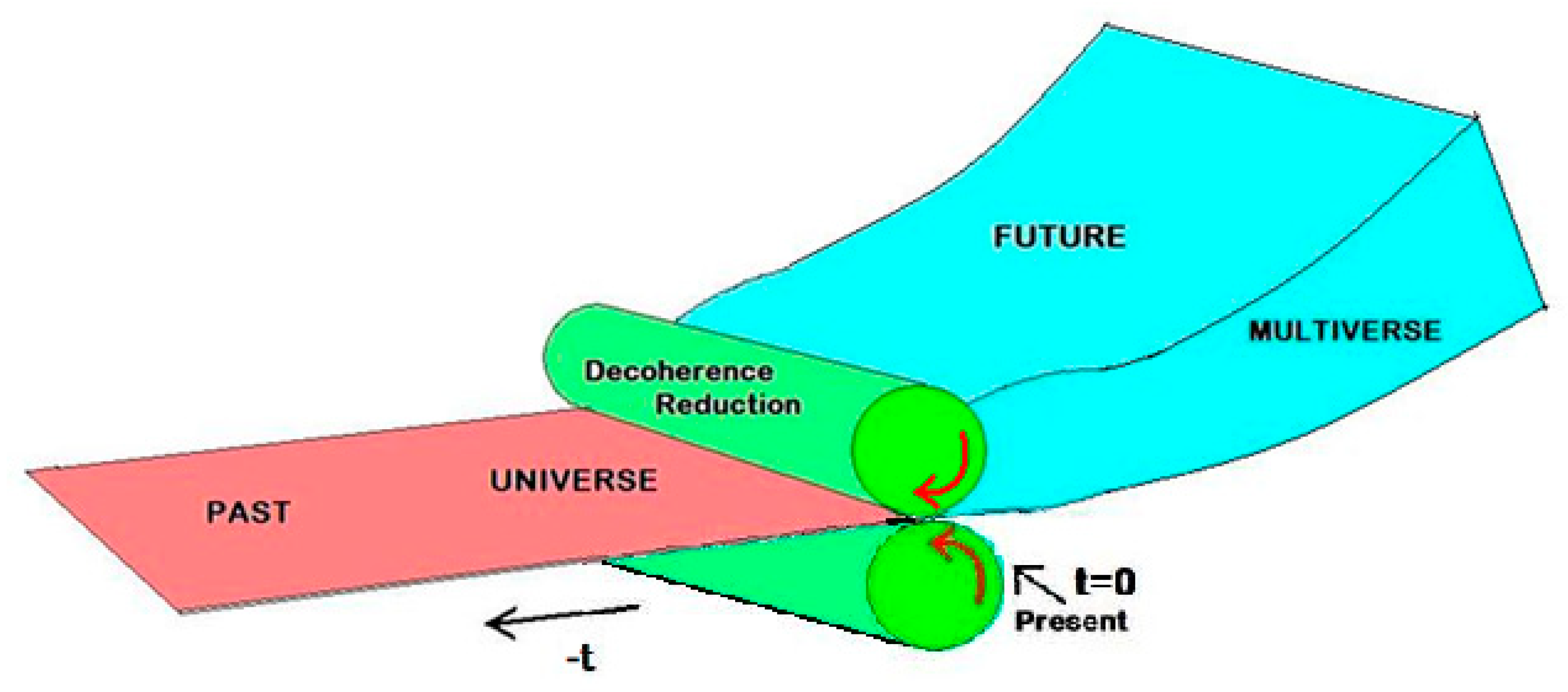
The 4D surface boundary between the future multiverse and the past universe marks the instant of present time. At this point, the irreversible process of decoherence occurs, entailing the computation or reduction to the present classical state. This specific moment defines the current time of reality, a concept that cannot be precisely located within the framework of relativistic spacetime. The moment in which irreversibility occurs distinguishes it from other points along the time coordinate and generates the experience of everyday real time.
4. Philosophical Breakthrough
The spacetime structure, governed by its laws of physical evolution, enables the modeling of reality as a computer simulation.
The randomness introduced by the GBN makes the simulation fundamentally unpredictable for an internal observer. Even if this observer uses the same algorithm as the simulation to predict future states, the lack of access to the same noise source quickly causes its predictions to diverge. This is because each fluctuation has a significant impact on the wavefunction's decay (see section 2.6.2-3). In other words, for the internal observer, the future is effectively "encrypted" by this noise.
If the noise driving the evolution of the simulation is pseudo-random but sufficiently unpredictable, only someone with knowledge of the seed would be able to accurately forecast the future or reverse the arrow of time. Even though pseudo-random noise can, in theory, be unraveled, the task of deriving the encryption key may be practically intractable. Therefore, with the presence of GBN, the outcome of the computation becomes "encrypted" by the high level of the randomness of this noise.
From this perspective, Einstein’s famous quote, "God does not play dice with the universe," takes on new meaning. Here, it suggests that the programmer of the universal simulation does not engage in randomness because, for he, everything is predetermined. However, from within our reality, we cannot access the seed of this noise, and thus it appears genuinely random to us.
Moreover, the laws of physics are not fixed or predetermined but rather the result of the settings of the simulation, which is designed to solve specific problems. For example, if we create a computer simulation of airplanes flying in the air, and we derive the behavior we observe—where the airplane stays in the air due to pressure on the wings—we derive the laws of gas aerodynamics. Similarly, if we simulate ships sailing, we observe and derive the laws of fluid dynamics. In the same way, the observed laws of reality are consequences of the purpose for which the universal simulation was created.
As discussed in § 3., if the aim of the simulation is to develop a physics that generates organized living structures through evolution—improving organization and efficiency—then the free will we exercise is simply the universe’s method of solving such a problem of "achieving the best organized and efficient possible future state."
From the programmer’s viewpoint, the simulation is progressing towards its intended solution through the method designed to this end. Inside the simulation, this manifests itself through a behavior we perceive as genuine free will.
4.1. Extending Free Will
At this point, a question arises: although we fortunately lack the omnipotent power to completely determine the future at will, and possess only free will limited to the near present, is scientific knowledge about the universe's evolutionary processes useful, and can it yield positive outcomes?
Although we cannot predict the ultimate outcome of our decisions beyond a certain point in time, it is feasible to develop methods that enhance the likelihood of achieving our desired results in the distant future. This forms the basis of the discipline of 'best decision-making.' It's important to highlight that having the most accurate information about the current state extends our ability to forecast future states. Furthermore, the farther away the realization of our desired outcome is, the easier it becomes to adjust our actions to attain it. This concept can be thought of as a preventive methodology. By combining information gathering and preventive methodology, we can optimize the likelihood of achieving our objectives and, consequently, expanding our free will.
Additionally, to streamline the evaluation process of 'what to do,' in addition to the rational-mathematical calculations that dynamically exatly e detailed reconstruct the pathway to our final state, we can focus solely on the probability of a certain future state configuration being realized, adopting a faster evaluation (a sort of Monte Carlo approach). This allows us to potentially identify the best sequence of events to achieve our objective. States beyond the time horizon in a realistic context can be accessed through a multi-step tree pathway. A practical example of this approach is the widely recognized cardiopulmonary resuscitation procedure [70,71]. In this procedure, even though the early assurance of the patient's rescue may not be guaranteed, it is possible to identify a sequence of actions that maximizes the probability of saving their life.
In the final scenario, free will is the ability to make the desired choice at each step, shaping the optimal path that enhances the probability of reaching the future desired reality. Considering the simulated nature of the universe, it becomes evident that utilizing powerful computers and softwares, such as those at the basis of artificial intelligence, for acquiring and handling information can significantly enhance the decision-making process. However, a comprehensive analysis and development of this argument extend beyond the scope of the current work and are deferred to future research.
5. Macroscopic Evolution and Far from Equilibrium Order Generation
Even if the quantum basis of the macroscopic universe evolution has been established so far and intelligence and consciousness are seen as inherent to its physical structure, we still do not have the scientific bridge between physics and biology.
The computational analogy highlights that the inherent physical laws we observe within a simulated reality result from the structure of the simulation algorithm, based on the problem it aims to solve.
One observed phenomenon driven by the physics of this reality is the tendency to generate matter self-organization and living systems.
At present, the physical law that establishes it is not yet fully defined and its formal structure is not well delineated. It has only been formulated for specific cases, such as atmospheric turbulence [6], electrochemical instabilities [5,9], stationary conditions not very far from equilibrium [1,2] and others particular cases discussed by Grandy [8].
In this section, we will show that, based on the SQHM, it is possible to define an energy-dissipation function whose stationarity governs the evolution of macroscopic irreversible behavior and possibly leads to order generation.
5.1. The Coarse-Grained Master Equation
From the general standpoint, discrete coarse-grained spatial description leading to master equation for a system evolition can be derived by the SQHM. When the elemental discrete cell is of order of the De Broglie length, eliminating the fast variables, we can derive the master equation by utilizing mass density current current , that by (74) reads
The macroscopic behavior can be obtained by the discrete coarse-grained spatial description of (90), with the local cell of side , which as a function of the j-th cell reads [40]
where
where
where is the spatial correlation length of the noise, where the terms, , and are matrices of coefficients corresponding to the discrete approximation of the derivatives at the j-th point.
Generally, the quantum potential interaction stemming by the k-th cell depends on the strength of the Hamiltonian potential .
By setting, in a system of a huge number of particles, the side length equal to the mean intermolecular distance, we can have the classical rarefied phase if is much larger than the quantum potential length of interaction(that by (5.12)) is also a function of the De Broglie length).
Typically, the Lennard-Jones potential (5.10) ( in the quantum limit) leads to
so that the interaction of the quantum potential (stemming by the k-th cell) into the adjacent cells, for a sufficiently large elemental cell, is null and is diagonal. Thus, the quantum effects are confined to each single-molecule cell domain.
Furthermore, for classical systems it follows that the spatial correlation length of the noise reads and the fluctuations appear spatially uncorrelated in the macroscopic systems
Conversely, given that for stronger than linearly interacting systems and the quantum potential of each cell extends its interaction to the other ones, the quantum character appears on the coarse-grained description.
As shown in §5.2, by using the stochastic hydrodynamic model (SQHM), it is possible to derive descriptions for dense phases where quantum effects appear on the macroscopic scale.
5.2. The Kinetic Equation Classical Gas and Fluid Phases
Once the from the SPDE (7) is defined, when the quantum coherence length goes to infinity (with respect the scale of our system or description), due to the suppression of mass density fluctuations by the quantum potential, since converges to it follows that tends to ans the SQHM converges to the quantum mechanics. In this case, acquire the full quantum meaning given by (1-4).
Neverthless, it is noteworhty to observe that the SQHM motion equations (7-9,14-16) have been derived [40] under the condition that the system’s physical length is close to the De Broglie wavelength. The main consequence of this approximation is that the noise in (7) depends solely on time, whereas, over macroscopic distances, it generally depends on both time and space.
Therefore, generally speaking, for macroscopic systems the SQHM model reads [40,48,72]
where the force noise owns the correlation function
where
and the quantum mechanical mass density distribution, in this case a stoìchastic variable, obeys to the conservation equation
When both and are very small compared to the physical length of the system (e.g., mean particle distance or free molecular path), the classical stochastic dynamics arises.
Given the physical length of the system, the macroscopic local dynamics is achieved for those problems where ∪ << and therefore . In this case, (see Appendix and references [40,48,72]) the SQHM leads to
where, and .
where the stochastic mass density conservation (102) as well as the force noise on large scale becomes a white noise whose correlation function (see (A.8) in Appensdix) reads
where the stochastic potential gives rise to the random force noise.
Moreover, given the association of the quantum hydrodynaimc representation, it is possible to define the phase space mass density that in classical limit reads
From (92) the force noise owns the characteristics of white noise in the macroscopic limit. Moreover, (90--93) demonstrate that fluctuations are inherent to macroscopic classical behavior and represent an ineliminable remnant of the quantum characteristics of spacetime subjected to gravitational background noise. Therefore, classical mechanics is merely a theoretical abstraction that is never fully realized in reality.This is a consequence of the nature of gravity and the quantum foundations of the universe.
In this case, when dealing with a system containing a vast number of particles interacting through a sufficiently weak potential (such as Lennard-Jones potentials), we can define a statistical local cell (with side length ) containing a huge number of molecules, quantum decoupled, that form a local system. Under this assumption, the overall system can be ideally divided into numerous classical subsystems with randomly distributed characteristics. All these subsystems are quantum uncorrelated, as quantum entanglement is confined within the domain of individual molecules.
This allows us to express the statistical distribution of these subsystems in terms of operators applied to a 'mother distribution ' based on SQHM (see Appendix) and, therefore, independent by the establishment of local thermodynamic equilibrium.
As shown in Appendix, for a gas or mean-field fluid phases, we can describe our system by the single particle distribution from which we can extract the statistical single particle distribution[72].
As is well established, defining the evolution law of requires an additional equation, that as shown in Appendix, for isotropic phases, can be assumed in the form
Equation (107) essentially plays the role of the Boltzmann kinetic equation in the form of Fokker-Planck-like equation. The deficiency compared to the Boltzmann kinetic equation lies in the lack of information about the structure of the diffusion coefficient, which is essential for giving to (107) full significance.
To address this, the standard approach introduces additional information about the diffusion coefficient through the semi-empirical assumption of a linear relation between flows and fluxes at local equilibrium. However, the local equilibrium approximation constrains the applicability of Equation (107).
In the current work, as illustrated in the subsequent sections, we deduce Equation (107) from the SQHM, thereby granting it extended validity, as the SQHM kinetics remains applicable even far from equilibrium.
5.3. The mean Phase Space Volume of the Molecular Mass Density Distribution
In order to grasp additional information from (107) we observe that (for gasses and meanfield fluids) on the basis of the SQHM we can identify three dynamics:
- I.
- The free enlargements of the molecular PMD within the mean volume available per molecule between two consecutive collisions,
- II.
- The molecular collision gives rise to the shrinkage of the molecular PMD to the reduced free volume available for the colliding molecules.
- III.
- The diffusion of the molecules, in term of their mean position, as a consequence of the molecular collisions,
The point I is justified by the fact that soon after collision the single molecule restart with its stochastic quantum dynamics undergoing both ballistic and diffusional expansion.
Point II is justified by the fact that the single molecules in their available volume (much larger than ) have classical characteristics so that they remain distinguishable maintaining the pertinency to their volume. In this case no superposition of states with closest molecules exist. Therefore, during collision while the molecules come near, their exclusive volume diminuishes up to a minimum. After that, the expansion kinetics of point I is undertaken.
As consequence of free expansions and shrinkages, the molecular PMDs will occupy in time a mean phase space volume in the phase space cell , where is the mean volume available per molecule. Therefore we can pose
where the mean molecular volume of the “i” molecules belonging to reads:
where . Moreover, since the mean PMD phase space volume occupied per molecule has to be a fraction of the phase space volume available per molecule we can pose
where is the number of molecules in .
The mean molecular volume (MMV) generated by SQHM dynamics (7) for a single molecule on distance when , is almost diffusional with diffusion coefficient (being the mean fluctuation amplitude parameter (temperature) of the SQHM fluctuations induced by the GBN on quantum potential on the PDF (16)).
Given that the time between two consecutive collisions (where the is molecular diffusion coefficient), it follows that since the MMV (111) is larger, higher the SQHM fluctuations, and the value of the molecular collision time is larger, smaller the diffusion coefficient , it follows that the parameter in (111) can be assumed of the form
where we have concisely stated .
The value of defines the constant setting the value of the free energy at thermodynamic equilibrium [72]
Moreover, by using the definition of the statistical distribution
and by using (107), from (111) for stationary states it follows that
The kinetics (114-116) of the SQHM at the supramolecular scale, for both rarefied gas and classical liquid phases, highlights two main processes in order to define their statistical state:
- The fluctuating hydrodynamic mass density with noise amplitude (temperature) , characterized by a diffusion coefficient at the sub-molecular scale;
- The thermal molecular motion, characterized by a molecular diffusion coefficient at the intermolecular scale.
Since it is well-established that quantum phenomena emerge as temperature decreases, the asymptotic zero-temperature state with thermodynamic temperature , corresponds to a pure quantum state in the SQHM model, where and also vacuum fluctuations are absent. This suggests that the reduction in quantum potential fluctuations is accompanied by an increase in quantum entanglement that also reduces the randomness of molecular motion, which generates thermal energy fluctuations. This can occur only if vacuum and thermal fluctuations are coupled with each other. Furthermore, since this coupling occurs via gravitational forces (see § 2), we can assume it is weak, allowing us to pose that
In the case where the thermal energy does not resolve the interanl structure of the molecules (typical for many gasses and fluids at room temperature) and they can be treated as structureless classically interacting point-like particles ( where is the mean intermolecular distance) with central-symmetric potential, the direction of variation of must be aligned with leading toand and therefore (117) can be simplified to
from where it follows that
and, at first order in , that
Therefore, by introducing (120) into the FPE-type kinetic Equations (A.43) (see the Appendix) we obtain
that at first order in simplifies as
5.3. Maximum Stochastic Free Energy Dissipation in Stationary States Far from Equilibrium
The existence of a well-defined -function far from equilibrium allows for the formulation of a formal criterion for evolution. Insights into the nature of the -function can be gained by noting that, at local equilibrium, it converges to the free energy (normalized to ) [72]. Rooted in the SQHM framework, we can conceptualize it as the normalized quantum hydrodynamic free energy (NQHFE).
In order to derive a general criterion to which NQHFE obeys, we observe that the total differential of
can be written as a sum of two terms, such as:
that we name "dynamic differential" and "stochastic differential" respectively. In (125) the stochastic velocity vector evolves through a pathway with negative increments of . Moreover, by utilizing (119) we can recognize that is anti-parallel to and, therefore, we can affirm that along the relaxation patheway
If we speak in term of the positive amount (traceable to free energy dissipation at local equilibrium, see (A.47) in Appendix) , we have that
It is worth noting that the validity of criterion (126) or (127) applies to structureless, point-like particles that do not undergo chemical reactions and interact through a sufficiently weak central symmetric potential (such as Lennard-Jones type potentials). Therefore, its generality depends on the accuracy of these approximations.
Nonetheless, starting from the more general condition (117), in the presence of chemical reactions and other dissipative contributions arising from asymmetries in interparticle interactions—as seen in structured fluids such as liquid crystals—it is, in principle, possible to redefine a functional whose stationarity determines the evolutionary pathway described by .
5.4. Stability and Maximum Stochastic Free Energy Dissipation in Quasi-Isothermal Stationary States
To clarify the practical significance of the criterion provided in (127), we analyze the spatial kinetics near and far from equilibrium to which it refers.
5.4.1. Spatial Kinetic Equations
By utilizing the standard mathematical procedure [44] we transform the motion equation (121) into a spatial one over a finite volume V.
Given a quantity per particle
its spatial density:
and its first moment
where , it is possible to obtain the spatial differential equation from (121):
that by choosing
where is the “mechanical” temperature defined as
where the constant can be obtained at thermodynamic equilibrium.
After some manipulations, for a system far from equilibrium in terms of chemical concentrations and mechanical variables, but at local thermal equilibrium, the hydrodynamic free energy at constant volume reads
where t and are the internal energy and the macroscopic kinetic energy of the system, respectively, where
where represents the “source” term
and the out of equilibrium contribution
where and , where and are the mean entropy and mean free energy of the local domain, respectively.
Moreover, by expliciting the terms , and that read
where is a vector perpendicular to the infinitesimal element of the boundary surface, and
where
Equation (134) takes on a well-defined meaning.
It is worth mentioning that for potentials that are not function of momenta, the term in (140), can be brought out of the integral.
5.5. Quasi-Isothermal Systems at Constant-Volume: Maximum Free Energy Dissipation
The significance of stationary quasi-isothermal states, far from equilibrium under constant volume conditions, arises from the operational context observed in living systems. The constant volume condition is attributable to the low compressibility of the fluids, such as water, and the polymers comprising these systems.
When considering the overall system (including both the system and its environment), the energy reservoir can sometimes sustain the system in a stationary state, even over long laboratory time scales, while the combined system (system and reservoirs) is relaxing towards global equilibrium.
Moreover, assuming both the system and the energy reservoir are at constant volume, and that the reservoir is thermally isolated (without loss of generality, we can assume the energy reservoirs are much larger than the system and operate on it in a reversible manner), the decrease in the reservoir's free energy equals the free energy transferred to the system through volume forces.
Given that for stationary states under approximate isothermal conditions at constant volume (with fixed walls), it holds that
and that
where the suffix “sur” and “vol” refer to contributions coming from the boundary surface and volume of the system , respectively. Therefore, from (134) it follows that
Moreover, given the quasi-isothermal condition, such that
and the far from mechanical and chemical equilibrium such that
Equation (137) reads
and, therefore, (145) reads
Moreover, assuming that the reservoir free energy transferred to the system, , is then dissipated by the system in heat such that (reversibly transferred to the environment (defined positive outgoing) through the surface at constant temperature such that: ) and, being for local thermal equilibrium that , for the energy conservation it follows that
and, finally, (149) that reads
Since for a stationary state both and are constant and is maximized with respect the variations of it follows thatis minimized with respect to the possible choices of . It should be noted that, since is not time dependent, this is possible because is not a total differential.
Therefore, for a classical phase of molecules undergoing elastic collisions and without chemical reactions at quasi-isothermal condition at constant volume, the system finds the stationary condition by maximizing its free energy dissipation.
5.6. Quasi-Isothermal Systems at Constant-Volume Without Reversible Free Energy Reservoirs: Maximum Heat Transfer
In general where it is not possible to control the free energy supply of the reservoirs, as for instance in the atmosphere instabilities, the free energy dissipation of the reservoirs is is not equal to of the system. Without the explicit form of the free energy dissipation, Equation (151) at local thermal equilirium simply reads
and it represents the principle of “maximum heat transfer” given by Malkus and Veronis [6] and holding for fluid dynamics and in describing the atmosphere turbulence.
It is worth mentioning that enunciation given by (151-152) shows that the principles given by Sawada and Malkus and Veronis are not of general validity but they are particular cases holding only in the case of quasi-isothermal conditions for an ordinary real gas (and its fluid phase) made of structureless molecules (e.g., classical rigid-spheres) sustaining elastic collisions and not undergoing to chemical reactions.
In fact, the general form (145)
hosts the term that is not always null and the terms , that are not generally constant.
5.7. Discussion of the Section
In far-from-equilibrium states, it is possible to define the hydrodynamic free energy and the hydrodynamic distribution functionthat describe the statistical state of the system and its kinetics.
Once the equations describing the evolution of the system are defined, the principle of maximal dissipation of the stochastic differential of the normalized quantum hydrodynamic free energy emerges in far-from-equilibrium stationary states.
This principle is not in contradiction with the previously mentioned principles of Prigogine, Sawada, Malkus, and Veronis; instead, it aligns with them, providing clarity to their intricate relationships. Our model illustrates that, in the case of real gases or Markovian fluids without chemical reactions under quasi-isothermal conditions, the principle results in maximum free energy dissipation, in line with Sawada's proposal, or in the principle of maximum heat transfer, as suggested by Malkus and Veronis. Simultaneously, for near-equilibrium stationary states, our theory indicates that the principle corresponds to Prigogine's principle of minimum entropy production.
The SQHM theory emphasizes that minimum entropy production and maximum dissipation of the hydrodynamic free energy (participant in the stochastic differential) are two distinct principles, each defined with respect to different variations. Nevertheless, both principles arise from a unified approach
The proposed principle underscores that free energy-based dissipation is the physical mechanism driving the emergence of order. Under far-from-equilibrium conditions, any system aiming to dissipate its hydrodynamic free energy, participant in the stochastic differentials, as rapidly as possible is forced to pass through a pathway where ordered configurations exist. The electro-convective experiments conducted by Sawada essentially serve as a demonstration of this principle under isothermal and isovolumic conditions.
6. From Order Generation to Living Organisms
The possibility of inducing order in classical phases, such as in fluids and gases, doesn't inherently result in the creation of stable well-ordered structures, with proper form, required for life. Achieving the stability and form retention akin to solids is crucial, and this necessitates rheological properties characteristic of solid phases. Thus, nature had to address the challenge of replicating the rheology of solids while retaining the classical properties of fluids or gases such as molecular mobility and diffusion.
The solution to this predicament lies in bi-phasic structures. Bi-phasic materials, such as gels, are composed of a solid matrix, often polymeric in living organisms, with pores filled by a fluid. In these formations, the solid matrix may constitute as little as 2-3% of the total weight, yet it imparts significant rubber-like elasticity to the overall structure, with a shear elastic modulus that, in gels containing interstitial fluids, can be on the order of or greater than . This generally far exceeds the modulus of aerogels, whose pores are filled with gas. Gels, due to their incompressible interstitial fluid, outperform aerogels in forming organized structures with solid consistency and complex functionalities [73], and were therefore preferred over aerogels in the development of living structures.
However, the path to the formation of living systems is far from straightforward, as the synthesis of natural bi-phasic materials was constrained by the availability of molecules present in the cosmic chemical environment.
Amino acids, produced through supernova activity, provided the building blocks for the solid matrix in the form of polymeric networks, which form the foundation of most living structures and tissues that host complex functionalities [73 and references therein]. Once gels established their role in the emergence of life, the next challenge was to develop an interstitial fluid that could be more versatile, widely distributed, and remain in a liquid phase at temperatures conducive to the energy-consuming and information storing of active functions of living systems.
6.1. The Fluid Problem
The availabilty of a fluid in the planetary configuration imposes some restrictions, here we itemize some possibilities:
- Europa (moon of Jupiter): Europa is covered by a thick ice crust, but beneath this ice, there might be a subsurface ocean. The exact composition of this ocean is not well-known, but it is believed to be a mixture of water and various salts.
- Titan (moon of Saturn): Titan has lakes and seas made of liquid hydrocarbons, primarily ethane and methane. The surface conditions on Titan, with extremely low temperatures and high atmospheric pressure, allow these substances to exist in liquid form.
- Enceladus (moon of Saturn): Similar to Europa, Enceladus is an icy moon with evidence of a subsurface ocean. The composition of this ocean is also likely to include water and possibly some dissolved minerals.
- Venus: Venus has an extremely hot and hostile surface, but some scientists have proposed the existence of "lava oceans" composed of molten rock. These would be much hotter and denser than typical water-based oceans on Earth.
- Exoplanets: The discovery of exoplanets with diverse conditions has expanded the possibilities for liquid environments. Depending on the atmospheric and surface conditions, liquids other than water and methane could exist, such as ammonia, sulfuric acid, or various exotic compounds.
Additional restrictions arise from the necessity of building up bi-phasic materials comprising a polymer network with intermolecular liquids. Beyond water, the idea of biphasic materials involving a polymer network and intermolecular liquids such as methane or ethane holds theoretical promise. However, its feasibility depends on several factors, including the compatibility of the materials and environmental conditions such as temperature and pressure.
6.2. The Information Storing Problem
As previously noted, polymer networks in biphasic materials offer structural support, while liquids (such as methane or ethane in this context) can act as a filler or component, imparting specific properties.
In the case of biphasic materials, several considerations come into play
- Compatibility: The polymer network and the intermolecular liquid should be compatible to form a stable biphasic material [73]. This may involve considering the chemical and physical interactions between the polymer and the liquid phase.
- Structural Integrity: The stability and structural integrity of the biphasic material over time need to be considered. Factors such as the potential for phase separation or degradation of the polymer network should be addressed.
Regarding the first point, it is crucial to evaluate whether amino acids can facilitate protein formation in alternative fluids, such as methane or ethane. This is because their various folding configurations in aqueous solutions enable the creation of an information storage mechanism through the folding-unfolding process. Beginning with a defined protein system (the chromosomal complement of an embryonic cell), an entire living organism is generated through a cascade process (unfolding set). Conversely, an individual living organism can preserve information about its structure by storing it in an encrypted format. A similar issue is currently under investigation in computer science, where researchers are seeking techniques to compress files to a minimal set of instructions (folding procedure), from which the complete original file can be extracted (unfolding). Therefore, the emergence of proteins in biphasic living structures represents another indispensable step towards the formation of complex living systems. On this matter, we note that the process of protein formation typically entails intricate biochemical processes taking place in aqueous environments. Proteins, as substantial biomolecules comprised of amino acids, undergo a highly specific and complex synthesis that hinges on the interactions among amino acids within aqueous solutions.
Methane, on the other hand, is a hydrophobic (water-repelling) molecule and is not conducive to the types of interactions required for the formation of proteins in the way we understand them on Earth.
Therefore, when contemplating the temperature and external pressure conditions necessary for ethane or methane to exist in a liquid phase—conditions that significantly influence factors crucial for life, such as the diffusion and mobility of chemical species it becomes evident that water, with its carbon-based chemistry, stands out as the most conducive fluid for supporting life. Therefore, we should anticipate that if any ordered structure is discovered in ethane or methane fluids, in presence of sufficiently high energy densities, it will not attain the complexity of those generated in water.
The processes of life, including the formation of proteins, are intricately tied to the properties of water as a solvent. In aqueous environments, amino acids can interact through hydrogen bonding and other forces to fold into specific three-dimensional structures, forming proteins. Moreover, protein folding is fundamental for information storage, which is fundamental in maintaining specific tasks and diversification of leaving functions in different organs or maintains information about the overall organizationof the living organisms necessary to establish its reproduction cycles. This process is also propaedeutic to the establishment of the selection process required for the perfectioning of living structures.
Nevertheless, while ethane or methane are not typically associated with the formation of proteins, it's worth noting that the search for life or the building blocks of life must not exclude the possibilities of alternative biochemistries that might exist in environments very different from Earth, such as those on moons or exoplanets even in simplest and rudimentary forms but with unexpected characteristics.
With this perspective, the solution for the existence of highly sophisticated living organisms lies in structures composed of aqueous gels. These structures not only provide support but also host active functions by facilitating the flow of ions and molecular species, generating maintenance or strengthening of the structure and information storing producing as final waste dissipation of free energy and products of associated reactions.
Basic active functions encompass various aspects, such as the mass transport essential for the plastic reconstruction of damaged tissues, organs or other living structures, the contractile muscle function responsible for macroscopic movements, the deposition of biochemical substances in neurons for information storage or to support psychological functions underlying consciousness [74] and so on. From this viewpoint, the continuous energy-based reshaping and treatment of information within living organisms are the driving forces behind life, making the material itself merely the continuously rebuilt and modeled substrate. It's noteworthy that this energetic back-function, wherein not only does the material substrate produce energy, but also the energy reshapes the material substrate, is the fundamental process that make living a system. Actually, the natural intelligence, consciousness, and intentionality are expression of this energy inverse role. This constitutes the insurmountable obstacle to achieving consciousness in artificial, so-called intelligent machines.
The difference between a living organism and an equal pile of atoms of carbon, hydrogen, oxygen, nitrogen and small quantities of salt is the energy flow: the first thinks, speaks and walks, the pile of the same quantity and type of matter does not. Being the matter substrate, wherein the life lies? All the specificity that we love in a person and living organisms is made by energy.
On this basis, we can also distinguish between the artificial intelligence of a machine and biological intelligence [74]: In the former, the unique chemical current is composed of electrons, and the "plastic" function of such currents is confined to the state of the computer bits.
6.3. The Sparking of Complexity Supported by Free Energy Ordering Force: The Intrinsic Natural Intelligence
The evolution of life towards more complex functions occurred with the availability of gel materials in a fluid environment, which assigned specific functions to specific locations, interacting with each other and defining the living system. In this manner, complex shapes associated with complex functioning emerged.
The acquired shape and ordered functions were maintained over time, enabling evolutionary selection to enhance order in organized systems. This specialization of functions contributed to the escalation of the pyramid of life's perfection involving the development of living organisms.
To have a overall picture it is useful to enumerate the items needed for the formation of living structures:
Level 1: Propelling force: Energy dissipation;
Level 2: Classical material phases:Temporary order generation in classical fluids and gasses;
Level 3: Mechanism of order maintenance and complex rheological structure formation: Stable order acquisition in bi-phasic structures (solid network filled by a fluid);
Level 4: carbon-based polymeric network in water solvent: the most functional system for energy/mass storage, reaction and transport.
Level 5: Information storing mechanism: Protein folding.
Level 1 is available and active throughout the universe, including in stars and black holes. Level 2 is widespread across planets and interstellar space in the form of hydrogen, water, methane, ethane, and other elements. Level 3 is possible on planets with a magnetosphere. Levels 4 and 5 are possible on planets located in the temperate zone around stars that have received debris and asteroids originating from supernovae.
The long chain of conditions leading to the emergence of living organisms with a high level of structural organization and functionality makes life a highly unlikely state, requiring numerous resources and components from the universe. It almost seems as if the entire universe is like a laboratory, purposefully prepared for this outcome
6.4. From the Generation of Ordered Structures to Living Structures
Indeed, the mere existence of a 'force' propelling material systems to organize themselves as rheological biphasic polymeric and protein gels, far from thermodynamic equilibrium, is not sufficient to generate living organisms; but a second stage is necessary.
It’s clear that order and structure are essential in the formation of living organisms. To grasp what life truly is — or to understand the difference between a collection of molecules and the same amount of matter in a living organism — consider the following thought experiment: if we were to hypothetically separate the molecules of a living organism, moving them far apart in a reversible manner, life would instantly stop. However, if we then return those molecules to their exact original positions, life would reappear. So, if the matter itself doesn’t change between these two states, what, then, defines life?
We can conclude that life arises from the interactions between its components, and is fundamentally an immaterial entity—primarily an energetic and informational phenomenon driven by the synergistic activities of its parts
From this perspective, we can generalize that the 'force' driving organization not only leads to the formation of living organisms but also to the emergence of complex social structures, shaping their behavior and dynamics. In this context, natural intelligence can be seen as a property inherent in all of nature and reality. Our goal here is to explain how the organizing tendency of energy naturally gives rise to processes—which we recognize as intelligent—focused on solving environmental challenges and identifying optimal evolutionary paths. This reveals a fundamental property of nature: without an environment, there is no intelligence.
Let's conduct a more in-depth analysis on this point. Let be the Hamiltonian function describing the j-th part of the living system or social structure. Then, the total Hamiltonian function of decoupled parts (when they are far away from each other) is given by:
Meanwhile, when the parts are interacting together in the “living” state, the Hamiltonian function can be formally thought composed by the contribution stemming from groups with increasing number of components such as
where refers to the additional energy due to the mutual interaction between pairs of molecules, between the triplets, and so on up to interactions between all molecules together. Therefore, the term:
is the term that refers to synergistic phenomena and is composed of terms concerning groups of elements whose number is
where is the number of particles in the considered group, is the total number of molecules or elements such as cells or individuals, for a total number of terms
which exhibits a quasi-exponential increase with the number N of mutual interacting elements.
The importance of synergistic terms in (156) naturally decrease as n increases in systems without particular symmetries. For instance, we can think to the first synercig term, in a social system that develops interaction between couples of individuals that is at the basis of reproduction while synergistic activities with three of more elements concern production of goods and life protection. Nevertheless, even the high order terms () contain terms that may give decreasing contribution, their number increase so quickly that the total effect can be of the same order of magnitude or bigger to be as importan as the preceding ones.
In fact, by considering the number of (158), for hugely large (as in complex living systems or social organizations) it can approximed by the formula
that reaches the biggest values for that read
whose exponential dependence can be better apprecciated in the formula,
that well expresses how the number of the N-th Hamiltonian term grows in exponential way in system with huge number of total components n.
This is true for the aboutcells of a biological system for which we have
but also for social aggregations like cities, or nations, with individuals for which it holds
Both numbers (162-3) are really huge and even if the contribution of the single term is very small compared to in (155) , the overal sum of them can furnish a relevant output. For instance, let’s consider the case where the mean sinergistic contribution in a city is of the single individual term such as
the total synergistic output
results much higher that the sum of the single outputs
with a gain ratio that reads
It should be noted that in large groups not each individual can directly interact with all others and therefore effective synergistic groups have usually . However, in highly organized systems like living organisms or cities, where it's common to see thousands or even tens of thousands of people engaged in collaborative activities, the synergistic contributions remain significant. With the advent of modern communication technologies, the number of synergistic interactions continues to increase very fast.
From this, we can infer that individuals living in a city would never be able to achieve, in isolation, what they can accomplish through coordinated efforts. This cooperation is essential for ensuring a comfortable and healthy life. The exponential growth in synergistic output also explains the rise of megacities, particularly in developing countries, where urbanization is a key driver for improving living standards. The synergistic perspective also clearly explains the positive effects of resources redistribution among different social categories of people
To illustrate the benefits of synergy, consider a simple example: a group of individuals facing extremely cold conditions. When they huddle together, the surface area for heat loss decreases, allowing them to survive in lower temperatures. On the other hand, if they were to remain apart, they would lose more energy and survival would become impossible under the same conditions. A similar principle applies to securing food in early human civilizations, which catalyzed the development of social structures.
In an agriculture-based early society with sparse populations, where families operate as mostly self-sufficient units, the synergistic effects are limited to a small number of individuals, leading to modest outputs. The want to have many children in such contexts arises from the need to increase the potential for synergy, although this effect is generally capped at around ten individuals.
The major turning point came with the rise of industrial society, where hundreds, thousands, or even hundreds of thousands of people could collaborate efficiently. This surge in synergistic activity spurred the wealth and well-being of modern civilization. These dynamics explain why people migrated from rural areas to cities and megacities, and why, paradoxically, poorer regions often have larger cities—a well-known global trend.
Furthermore, in industrial cities, the dense population and industrial infrastructure satisfy the need for synergy, reducing the necessity for large families. As a result, populations in industrialized societies tend to stabilize or even gradually decline. However, this effect is offset by the increasing efficiency of farmers, who require fewer and fewer workers to produce the same output. This solution offered by natural intelligence can increase personal income and health without increasing the total consumption of Earth's resources, which are finite
It’s also important to recognize that while energy is a conserved quantity and, therefore, the increase in output from energetic resources is proportional to the number of active elements, whereas the increase in output from organization grows exponentially. Given that Earth's system is finite, organizational synergy is the key mechanism capable of generating growth and improvement at constant energetic expences. Therefore, it should be the primary focus of any political system and ecological transition strategy.
Although not fully understood, this concept is embedded in the universal simulation and has been continuously pursued over time. The dynamics described here do not result in a static state; instead, they drive the development of ever more efficient systems, capable of overcoming increasingly difficult challenges and propagating themselves throughout the real world.
In this way, a natural selection mechanism is spontaneously embedded within living and social systems. This inherent drive for improvement in organized structures and their functions represents a form of natural intelligence that permeates universal reality and drives its evolution.
6.5. The Emergent Forms of Intelligence
Considering intelligence as a function that, in certain circumstances, aids in finding the most effective way to achieve desired or useful outcomes, it's conceivable that various methods beyond slow and burdensome rational calculations exist to attain results. This concept aligns with emotional intelligence, and at deeper level with consciusness, a basic mechanism that, as demonstrated by psychology and neuroscience, initiates subsequent purposeful evaluation [75,76,77,78].
The simulation nature of reality demonstrates a form of natural intelligence has evolved through a selection rule based on the assumption that 'the winner is the best solution'. At a fundamental level, the emergence of living systems is rooted in the physical laws governing matter self-assembly driven by free energy dissipation. Here, efficiency plays a crucial role, improved by a process that we can identify as natural intelligence.
Nevertheless, this criterion does not lead to a unique outcome, as two methodologies emerge. The first is 'captative intelligence,' in which the subject acquires resources by overcoming and/or destroying the antagonist. The second is 'synergistic intelligence,' which seeks collaborative actions to share resources or build a more efficient system or structure. This latter form of natural intelligence has played a crucial role in shaping organized systems (such as living organisms), social structures, and their behaviors. However, a thorough examination of the dynamics produced by these intelligent approaches requires additional information and will be addressed later in the paper.
6.5.1. Dynamical Conscience
Following the quantum, yet macroscopically classical dynamics of the SQHM, all objects—including living organisms—within the simulation analogy undergo re-calculations (definition of their classical state) in each local quantum domain at every time step after decoherence. This process propels them forward into the future within reality.
In ordered systems capable of managing energy and information, such as living organisms—whose formation is also encoded in the physical laws derived from the settings of the universal simulation—the compilation of previous instantaneous states, stored and processed to provide expectations for future moments, encapsulates the dynamics of evolution and forms the basis for consciousness in living organisms [76,77,78]. Furthermore, in the universal simulation’s task of achieving the optimal future state—in terms of generating order and maximizing information conservation (a potential definition of natural efficiency)—consciousness in living organisms serves as the foundation for free will. From this perspective, consciousness and free will, though present to varying degrees in living organisms, are not exclusive to humans but are also possessed by animals and in different forms by all living organisms.
Various accepted models in neuroscience conceptualizes the consciousness of the biological mind as a three-level process [75,76,77,78]. Starting from the outermost level and moving inward, we have the cognitive calculation, the orientative emotional stage, and, at the most fundamental level, the discrete time acquisition routine. This routine captures the present state, compares it with the anticipated state from the previous time instant, and projects the future state may coming from the next acquisition step. The comparison between the anticipated and realized states provides input for decision-making at higher levels. Additionally, this comparison generates awareness of changes in reality and the speed of those changes, allowing for adjustments in the adaptive time scan velocity. In situations where reality is rapidly evolving with the emergence of new elements or potential dangers, the scanning time velocity is increased. This process gives rise to the subjective perception of time dilation, where a few moments appear as a significantly prolonged period in the subject's mind. It is also worth mentioning that distortions in predicting future states are at the root of many psychological pathologies.
Considering the inherent nature of universal time progression, where optimal performance is attained through the utilization of quantum computation involving stepwise quantum evolution and wavefunction decay (output extraction), it becomes inevitable that the living system, optimized for maximum efficiency, inevitably adopts the highest-performing intelligence for a sub-universal system (the minds of living organisms) through the replication of the smart universal quantum computing method. This suggests that groups of interconnected neurons implement quantum computing at the microscopic level of their structure, resulting in their output and/or overall state being the outcome of multiple local wavefunction decays.
The macroscopic classical reality, characterized by microscopic discrete space-time quantum domains, aligns with the Penrose-Hameroff theory [79] proposing that a quantum mechanical approach to consciousness can account for various aspects of human behavior, including free will. According to this, initially the brain utilizes the inherent property of quantum physical systems to exist in multiple superposed states, allowing it to explore a range of different options (or multiple sensorial inputs) in the shortest possible period of time and then the decision is obtained (i.e., “calculated”) by the decoherent decaying to the macroscopic (unique) neuronal state.
6.5.2. Intentionality of Conscience
Intentionality is contingent upon the fundamental function of intelligence, which empowers the intelligent system to respond to environmental situations. Following calculation or emotional evaluation, when potential beneficial objectives are identified, intentionality is activated to initiate action. However, this reliance is constrained by the underlying laws of physics explicitly springing forth the task the universal simulation has been set for. Essentially, the intelligent system is calibrated to adhere to the physics of the simulation perhaps proceeding by utilizing the same universal computing method: proceeding to the next instant through evolution of quantum superposition of states (nonlocal grouping of information coming from various parts of living system placed in different places of the space) and then derivation (calculation) of the next classical state (decision or stable convincement) by the decay to a stable (classical) state.
Generally speaking, in our reality, conscience, intelligence and free will address all needs essential for development of order, namely life and organized more and more efficient structures, encompassing basic requirements, for instance, such as the necessity to eat, freedom of movement, association, protection from cold and heat, maintain the integrity of its structure, or functions, and many others.
This problem-solving disposition is, however, constrained by the physical interaction with the environment. From this perspective, when we consider artificial machines, it becomes clear that they cannot develop intentionality solely through computation, as they lack integration with the real world. In biological intelligence, structure is deeply connected to the environment through the physical processes that drive reality forward. The living (or intelligent) system not only manages energy and information but also engages in a reciprocal mechanism: energy shapes and develops the 'wetware' of living organisms [74], including the structures responsible for intelligence.
In contrast, a computational machine lacks the capacity to autonomously modify its hardware and establish criteria for its safe maintenance or enhancement. In other words, intentionality, the driving force behind the pursuit of desired solutions, cannot be developed by computational procedure executed by immutable hardware Intentionality serves as a safety mechanism, or navigation system, for a continually evolving intelligent system whose structure and functionality are seamlessly integrated with the environment and continuously updated. To achieve this, a physically self-evolving plastic wetware is necessary [74].
6.5.3. On Computability of Conscience
If we define the concept of consciousness computability as the ability to replicate the mental evolution, self-perceptions, potential actions, and decision-making processes of living organisms, we noted in the previous section that at least three elements are involved: self-evolving wetware, the environment (to which it is intimately connected), and short-term quantum non-loca evolution followed by decay into a classical state through decoherence. This final process, in line with current thinking [75,79], is essential for the formation of a unified, non-local representation (or consciousness) of reality.
This assertion definitively excludes the possibility of classical computability of consciousness. While rational chatbots can be developed using trained neural networks to mimic mental behavior by generating and deriving the most probable configurational outputs, predicting the beliefs and decisions of living organisms (whether animals or humans) necessarily requires the use of effective quantum-based computational algorithms. From this perspective, the development of quantum computing neural networks must focus on ensuring effectiveness. Although we may not fully understand the 'computational algorithm' inherently embedded in qubits, we can still use them empirically for building quantum computers and related quantum computing systems. However, challenges remain in creating large-scale qubit systems, error correction procedures, and the development of faster quantum computation methods, which are essential for accurately mimicking 'real-time' behaviors.
In principle, the theory described in sections 2.6.1–2 could enable the classical computation of an algorithm that mimics the functioning of qubits, thereby allowing classical computation of quantum phenomena such as conscience. However, the real challenge lies in the efficiency of these calculations, particularly in relation to the scalability of the problem. The significant time and energy expenditure required to implement such a theoretical model makes the classical computation of quantum phenomena non-scalable, rendering it an NP problem.
A striking example is that chatbot machines, which process human conversations and information transmissions, consume megawatts of energy. As the demand for computing resources grows exponentially with data complexity, enhancing their capabilities to add functionalities such that also conscience can be replicated, is currently unfeasible. Therefore, quantum computing becomes essential to potentially have a scalable problem transforming NP problems, such as to replicate the conscience, into P problems.
On the other hand, the mind's efficiency in producing its behavior using just two teaspoons of sugar—equivalent to 240 kilojoules per hour (less than 0.1 watts of energy consumption)—reveals the hidden use of the efficiency of quantum algorythms of operation.
6.5.4. Final Considerations of the Section
Considering that the maximum entropy tendency is not universally valid, but rather the most efficient energy dissipation with order and living structures formation is the emergent law [72], we are positioned to narrow down the goal, motivating the simulation, to two possibilities: the generation of life and/or the realization of efficient intelligent and conscient systems.
As the physical laws, along with the resulting evolution of reality, are embedded in the problem that the simulation seeks to address, intentionality and free will are inherently manifested within the reality to achieve the simulation's objective.
Furthermore, the conscience is deeply rooted in the quantum basis of the discrete large scale classical reality utilizing the same algorithm the universe adopt for proceeding forward in time.
Classical computation relies on deterministic logics and predefined algorithms, which make it difficult to fully simulate complex phenomena such as consciousness, which involve the simultaneous integration of numerous inputs and a nonlinear adaptive response. The hypothesis that consciousness requires quantum computation rely on the inherent complexity of mental processes and the nonlocal and interconnected nature of consciousness. Quantum computing, with its ability to perform computations in parallel and handle superposed and entangled states, could theoretically offer a platform to model these complex processes. Even if consciousness requires quantum processes, we are still far from being able to build quantum systems that are sufficiently stable and scalable to simulate complex cognitive functions or even consciousness. Current limitations in error correction, decoherence, and the integration of large qubit networks present significant obstacles.
6.6. The Glucose-Insulin Control System: Insights from Natural Intelligence for Economic Science
An interesting strategy that natural intelligence has been able to build up is the glucose-insulin control developed in high-level living organism [80].
In figure 2 we can see the response of insulin blood concentration to a step infusion to glucose. As expected, along time the insulin concentration grows in order to lower the glucose content, but what is relevant is the initial peak of insulin at the starting of glucose infusion. This is explained by the Fisher algorithm that model the insulin response in figure3. sensible also to the velocity of glucose variation. This initial overestimation is useful for increasing the speed and efficiency of the glucose normalization. The amount of insulin released is far greater than what is immediately required for the current blood glucose concentration. This can be seen as a strategy that accounts for the inertia in the reaction-diffusion dynamics of bodily fluids, anticipating the desired effect.
6.6.1. Application of Natural Intelligence in the Economical Dynamics
It is interesting to note the efficency and usefulness of the insulin delivery strategy in order to control the glucose blood concentration by applying the same strategy to the control of inflaction in economical systems. To this end, we can associate glucose to inflaction and the interest rate of monetary system to insulin, where the latter hampers the former.
Generally speaking, the above dynamics belong to those following the prey-predator skeme described by the Lokta-Volterra differential equation.
In the economical dynamics, the pray is constituted by the availability of money among individuals that is used for investments and consumptions. On the other hand the predator is the interest rate for borrowing the money: higher is the interest rate larger is the picking up of money from the free circulation and vice versa.
Higher is the profit of banks from borrowing money, lower is the availability of money in the financial circuit. When the economical slow-down induced the lacking of money lowers the profits, the banck debitors will stop reinbursements so that they have to lower the interest rate to let the pray (money density in the society) increase so that investment and production can restart and the banck (predator) can have the pray (money) to eat.
From this basic sckeme, thence, the insulin blood concentratio corresponds to the interest rate and the glucoce concentration to the money availability in the economical system.
Forllowing the model of pray-predator dynamics, recessions and economical expansions are the consequences of the over-damping of pray and predator respectively. When predators (high interest rate) withdraw too money from the economical circuit, the economical activities slows down or even stops. Thence, also predators may get troubles if the money distruction is too strong and have lower income or even shut down. In order to stop this dynamics the finalcial control system is forced to lower the interest rate of maney borrowing restart to increase.
It must be noted that this model in which the system structure is assumed as invariant. This means in the insuli-control system that we do not consider the possible damaging induced by a severe. In the economical model this correspond to the condition that the economical structure remains functioning and not damaged that is to say that a hramful deindustrialization is not considered.
Therefore, in the economical model, we have to introduce the condition that recessions is moderate and do not produce damage to the society structure. This constitutes the fundamental difference between recession and depression, the first one is useful and leads to the imrovement od society efficiency, the second one is deleterius and leads to desctuction and loss of society efficiency.
6.6. Biomimetic Control of Inflation
In Figure 4, we observe the pattern of inflation in response to the typical scenario of increasing interest rates to mitigate it. The rate of change of inflation slows down progressively as the disparity between the equilibrium interest rate and the current rate widens. Subsequently, the beginning of inflation decline is asumed as the signal when to start to lower the interest rate. Even if the interest rate is subsequently reduced, due to inertial effects, the pace of inflation decrease remains relatively rapid pushing the inflactin too low or even the system in dangerous deflaction. Additionally, due to the constraint that interest rates cannot effectively fall much below zero, the lowering of inflation becomes notably arduous to reverse and protracted over time.
In Figure 4, The decrease in inflation follows the gradual rise in interest rates. This decline is not immediate; due to inertial effects of monetary dynamics, it occurs only after interest rates reach a peak significantly above the equilibrium level. At this point, inflation drops sharply, even as interest rates begin to fall, which may push inflation dangerously close to deflation
Figure 5.
Inflation dynamics following step increases in interest rates, with temporary gradual decreases occurring before inflation begins to decline, help moderate the long-term downward trend in inflation..
Figure 5.
Inflation dynamics following step increases in interest rates, with temporary gradual decreases occurring before inflation begins to decline, help moderate the long-term downward trend in inflation..
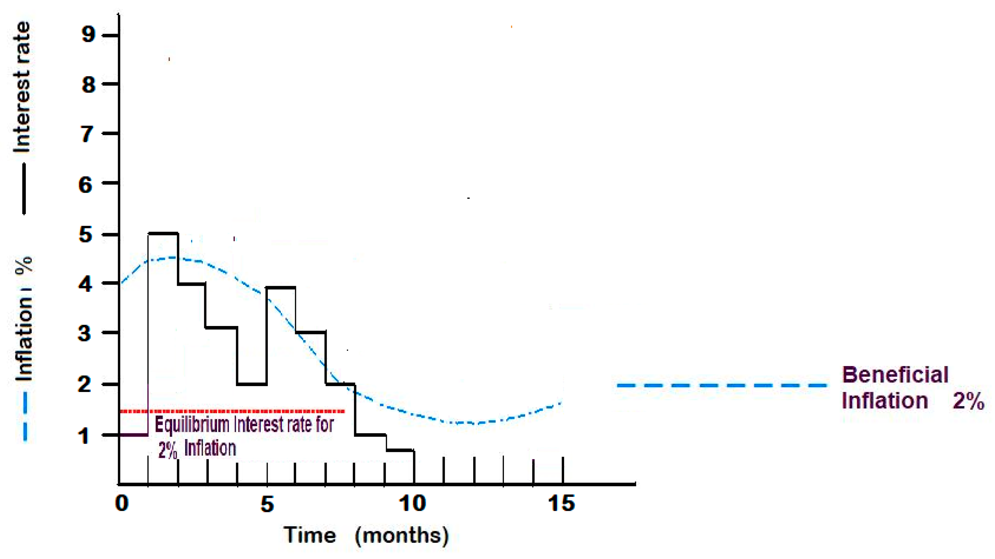
6.7. The Usefulness of Economic Recessions
One of the major debates in economic science revolves around the role of recessionary phases. While the significance and usefulness of expansive economic stages are widely understood—where investments aimed at boosting production output in terms of goods and services are considered the natural course of action—opinions regarding recessionary economic periods are varied. Many individuals believe that recessions are inherently negative and should be avoided altogether. However, from the perspective of how reality unfolds, it can be argued that these economic phases play an important role.
During a recession, consumption typically slows down, and businesses experience reduced incomes, often leading them towards economic failure. However, experience demonstrates that enterprises emerged from recessions has developed a new organized structure that maintain the same output with fewer expenses, or alternatively, produce more and different goods, with the same financial outlay. In doing so, they avoid failure and are able to continue paying salaries, sustaining consumption levels. As this attitude sparks around all the society, the consumption stops to diminish as well as workers firing tends to halt. In essence, recessionary economic phases stimulate an increase in the efficiency of the production system.
It is worth mentioning that, since energy is conserved, the energetic output grows linearly with means of production of the system, while the organization can exponentially increase the output at constant energy consuption. This clearly makes the economical recession phases more important that the expansive ones in term of social progression and shows that the main task of the central power is to increase the efficiency of the society through constant organizational action.
Hence, if expansion is characterized by an increase in the production system and is energy-intensive, recession represents a phase focused on efficiency enhancement, where restructuring of productive resources becomes paramount. However, it's essential to differentiate between various types of recessions: moderate recessions and severe recessions that are commonly referred to as depressions. In the case of a depression, the recession is so severe and profound that it disintegrates collaborative activities, among peoples leading to the collapse of social organization and structures with irreversible damage. As a result, the productive system suffers irreparable destruction, making restructuring for efficiency enhancement much more difficult. Businesses lay off workers, who remain idle at home and lose their skills. This causes a sharp decline in social efficiency, rather than growth. Instead of the continuous reshaping of society through restructuring of work systems, there is a genuine collapse, severely impoverishing the means of production, severe drop of synergies among people and reconstruction of social organization.
From the perspective of the synergistic behavior within modern societies, we can grasp the actions necessary to prevent recessions from descending into depressions. When workplaces, where workers collaborate synergistically, are shuttered and their members dispersed throughout society, often resulting in angry protests, it parallels the damage inflicted on cells by trauma, where their contents spill out, causing inflammation within the body. Just as in a living organism in which we preserve the vitality of cells, in the economic fabric, we must sustain the synergy among people. It's imperative to avert the collapse of enterprises at all costs: Financial institutions, workers' associations and governmental authorities, must collaborate to preserve the capacity of workers to collaborate effectively despite monetary discrepancies and shortfalls in financial records.
Frequently, the downfall of an enterprise stems from a mere "book" issue, where numbers fail to adhere to rigidly defined rules, often resulting in insignificant amounts compared to the ensuing damages caused by their enforcement. During severe recessions, it becomes crucial to set aside economic formalities and focus on preserving productive structures through restructuring
7. Imperfection and Shortcuts of the Evolutionary Selection
Until now, we have explored the natural forces driving the creation of ordered structures and living systems. The spontaneous tendency of energy to manage information, represents a form of natural intelligence. This intelligence is an expression of the universal algorithm developing the reality progression, aimed at perfecting and increasing the efficiency of living systems or structures over time.
Nonetheless, the selection rule that produces the organization improvement employed by natural evolution, at the nowadays stage, is not free from side effects and can result in shortcuts that lead to disorganization and destruction. The selection criterion that is based on the rule: “Who prevails is the best “ can be exploited in two distinct ways: the first, which is based on a 'synergistic methodology,' involves individual entities (such as people or biological cells) collaborating to obtain resources and then sharing them; The second method, based on a 'stealth methodology', involves destroying other individuals to seize their resources.
Synergistic intelligence and stealth intelligence produce distinct outcomes and dynamics. As the proportion of individuals in a society with synergistic intelligence increases, system efficiency and organization improve. In contrast, stealth intelligence is unsustainable; as more participants adopt it, system efficiency declines drastically, leaving individuals with insufficient resources. If 100% of people operate with stealth intelligence, with everyone taking from others without contributing, the system becomes unsustainable, leading to total collapse and the demise of everyone. People with stealth intelligence depend on those with synergistic intelligence, but not the other way around.
In the short term, this behavior mirrors a Volterra-Lokta dynamic, where an increase in individuals with stealth intelligence (the predators) cannot grow indefinitely. Eventually, a plateau or decline occurs, allowing for a resurgence of individuals or systems with synergistic intelligence (the prey). However, over a very long-time scale — one that matches the timeframe of the universal simulation's search for a solution — stealth intelligence, being self-contradictory, cannot persist indefinitely or be adopted by all individuals within the system. Meanwhile, synergistic intelligence can, in principle, endure indefinitely with all individuals adopting it, leading to continuous improvement in a universal system. Therefore, synergistic intelligence will ultimately prevail, representing the unique, self-consistent, stable endpoint of the universal simulation.
In practice, synergistic individuals drive constant progress in their systems, but their success, which leads to widespread prosperity, makes the stealthy approach more tempting and fruitful for others, especially those who lack long-term perspective. This dynamic holds in the presence of small fluctuations or gradual changes within the system, persisting until a major environmental shift or catastrophic event leads to system collapse. At that point, a new era may begin, with different intelligent organisms and systems tested to see if they can develop superior intelligence (capable of better dealing with stealthy individuals) or more effective forms of collaboration.
7.1. War-Peace Cycle
The conflicting dynamics between synergistic and stealth intelligence within human societies form the basis of the war-peace cycles observed throughout history. During periods of war, society plunges into a state of extreme deprivation, where individuals lack resources and struggle even to find food. The destruction of a people to gain practically no resources forces individuals to collaborate synergistically, exchanging labor and cooperation for survival. When war ends due to the exhaustion of resources and means, the mentality of collaboration has became dominant, and this leads to an increase in productivity and advancement in all fields of human activity.
However, after a number of years, as society becomes populated with wealthy individuals and a new generation arises without the lived experience of wartime collaboration, the pursuit of wealth through aggressive means—attacking, assaulting, and plundering others—becomes appealing once again. We see strong recent evidence of this in post second world-war period. In the 1970s and 1980s, world leaders focused on treaties of cooperation and military limitations, while in more recent times, aggressive rhetoric and warlike posturing have re-emerged on the international stage.
Interestingly, this cycle mirrors the economic phases of recession and expansion, where recessions serve as a prelude to the next wave of growth based on improved efficiency. In this context, the increased efficiency (a healthier society) results from the educational impact of war on the people, fostering the benefits of synergistic intelligence. Evidence of this can be seen in the fact that major wars often follow periods of deep economic depression.
7.2. Triggering of Destroying-Reconstruction Regime
Excessively free-market economic systems, which are built on the assumption of exponential (or at least continuous) growth, lead to the rise of increasingly powerful financial groups. These groups, by exerting significant influence over political leadership and national media, impose their own interests on society in ways that, while legal, effectively limit or eliminate individual freedoms. In practice, the industrial system is incentivized to strip people of independent sources of sustenance—such as food, work, energy, and transportation. Arable land is pseudo-legally taken from farmers through increasingly restrictive regulations. Instead of supporting natural biofuels, industries promote electric and hydrogen alternatives, replacing widely available natural resources that could provide income to everyone with options that require industrial involvement. This creates a dependency on industrial products and establishes, through legal means, a form of oligarchic industrial monopoly.
Furthermore, traditional methods of home heating, such as firewood—which operates on a neutral carbon dioxide cycle—are being banned to allow industries to emit more fossil CO₂. Though this may seem justifiable in environmental calculations, leaving carbon stored in unused forest wood reduces forest management, leading to more intense wildfires that release more CO₂ (all that one stored in unused wood). The rise in carbon dioxide from wildfires cannot be accurately accounted for in emissions calculations, creating a misleading picture where emissions appear stable on paper, but in reality, they increase due to the unchecked growth in wildfire intensity.
However, the harmful actions of stealthy intelligence by large industrial groups in overly liberal economic systems are not limited to these examples and can be even more damaging. One such example is planned obsolescence, where products are intentionally designed with shortened lifespans to artificially limit their functionality. Worse still, in a world where continuous growth is unsustainable, the drive to maximize profits ultimately requires phases of destruction to make space for new reconstruction and renewed exponential growth. This results in a growing tendency to incite conflicts around the world—an approach that becomes more effective as people forget the value of collaborative intelligence, which fosters slower, but more sustainable, growth while ensuring social and psychological well-being, rather than the loss of countless lives.
7.3. Final Considerations
Once the physical laws governing the evolution of complex systems are understood, it becomes possible to analyze the development of life and its associated social structures and dynamics. On shorter timescales, where the biosystem experiences minor fluctuations, the system progresses through increasing order and efficiency. However, on longer timescales, larger fluctuations may occur, potentially leading to collapses and catastrophic events. These events can be conceptualized as phenomena like a universal flood, a large asteroid impact, or an apocalyptic event such as nuclear war—causing sudden disruption of organized structures and their environments.
The emerging picture suggests that evolution, driven by natural physical laws, follows a cycle of 'proliferation and garbage collection,' a concept well defined in computer programming and also applicable to contemporary societal dynamics. Societies expand and grow under the influence of synergistic intelligence. During this period, various parasitic individuals and organizations develop uncontrollably. While moderate stealth intelligence may institutionalize itself in the short term, catastrophic events followed by collapse and destruction act as a form of natural selection, clearing the way for new entities capable of surviving the disaster—entities that would never have emerged without it.
This raises the question: Is humanity bound to an inevitable fate, or is there an escape route? Nature, functioning like a vast computer simulation, offers an answer: If present civilization collapses, I restart the simulation to seek new solutions; if it manages to avoid collapse, I continue refining the current solution. Thus, humanity's task is to earn its survival.
Achieving this goal requires a deep understanding and broad application of the physical laws that underpin life and the generation of well-being.
8. Conclusions
The stochastic quantum hydrodynamic model represents a major breakthrough by integrating the effects of a fluctuating gravitational field, similar to dark energy, into quantum equations. This innovative approach provides solutions that address key challenges in both macroscopic phenomena and quantum physics. Beyond the quantum potential interaction range, it cannot maintain the coherent Schrödinger behavior of the wavefunction's outer regions. Notably, the theory finds experimental support through the validation of the Lindemann constant, related to the melting point of solid lattices and the transition from fluid to superfluid phases.
The self-consistency of the SQHM is ensured by its capacity to describe wavefunction collapse within its theoretical framework. This feature enables it to reconcile the relativistic principle of locality with the non-local nature of quantum mechanics, specifically linking the uncertainty principle to the speed of light as a maximal limit. Additionally, by showing that large-scale systems self-decay into stable, decoherent states, the SQHM provides an effective solution to the issue of 'pre-existing' reality in quantum mechanics.
The paper goes on to illustrate that the physical dynamics of the SQHM can be likened to a computer simulation, where various optimization processes are employed to bring it into existence. This framework, which leads to a macroscopic reality with a foam-like structure—where microscopic quantum domains coexist—offers insights into the nature of time in our current reality and enhances our understanding of free will. The model proposes that irreversible processes shape the manifestation of macroscopic reality in the present moment, suggesting that the multiverse exists only in future states, while the past is composed of the universe formed after the present instant. The projective decay occurring in the present serves as the mechanism through which the multiverse collapses into a single universe.
The discrete simulation analogy provides a framework for addressing several fundamental questions. It unveils a strategy that reduces the amount of information to be processed, thereby enabling the generation of reality. It emphasizes that reality is the outcome of a simulation designed to solve a specific, predefined problem, meaning that the physical laws we observe are merely a consequence of this requirement. In this context, the simulation seems to follow an entropic optimization strategy, aiming to minimize information loss while maximizing useful data compression and preservation. This approach aligns with the simulation’s purpose of generating living organized systems, intelligence, and consciousness. On this basis, while the physical law governing matter's self-organization is embedded within the generated reality, it remains incomplete.
To fill this gap, this study has developed an extremal principle that governs the far-from-equilibrium evolution of systems composed of structureless particles by utilizing the stochastic quantum hydrodynamic analogy. For classical phases, where quantum correlations decay over distances shorter than the average inter-molecular separation, we demonstrated that the far-from-equilibrium kinetic behavior can be captured by a Fokker-Planck equation. The derived velocity vector in phase space maximizes the dissipation of stochastic free energy, a function analogous to energy, thus providing a framework for understanding energy dissipation in such systems. In quasi-isothermal, far-from-equilibrium states without chemical reactions, this approach simplifies to Sawada's principle of maximum free energy dissipation. However, when chemical reactions or significant thermal gradients are involved, the work uncovers additional dissipative contributions. The results also demonstrate that the Malkus and Veronis's principle of maximum heat transfer is a special case within this theoretical framework. As systems evolve towards equilibrium, in order to maximize the dissipation of stochastic free energy they are forced to pass through progressively ordered states, thus facilitating the self-organization of matter.
However, the paper also emphasizes that self-organization in fluids and gases alone is insufficient to give rise to complex living structures. These structures require additional conditions for their emergence, such as the ability to
- preserve acquired organization over time;
- possess solid-like rheological properties to enable the expression of complex shapes and diverse functions distributed across space;
- have the capacity to store information to support functions such as self-repair, reproduction, and intelligence.
To achieve all these goals, the universe functions as a vast laboratory for the creation of living organisms.
The study highlights how synergistic effects and tendencies toward efficiency drive evolution, revealing intriguing parallels between biological and social systems. The findings put in evidence that natural intelligence, consciousness, and free will are intrinsic properties of the universe’s physical evolution, though they are accompanied by various side effects. Regarding intelligence and consciousness, two possible approaches—stealthy intelligence and synergistic intelligence—are possible to solve the problem of achieving the 'best future state' complicating progress toward efficiency and prosperity. As for free will, the work shows that it exists but is limited in time and cannot be absolute.
This work demonstrates that neither determinism nor pure probabilism underpins the physical evolution of the universe. It shows that probabilism, introduced into quantum mechanics—a theory with a fully deterministic mathematical framework—arises from the gravitational foundations of spacetime. These foundations generate a fluctuating background that leads to the unpredictable collapse of the wavefunction. At the same time, the SQHM framework reveals that deterministic classical mechanics does not truly exist; rather, it emerges as a macroscopic phenomenon in which residual fluctuations of the quantum potential are always present and unavoidable.
Thus, we are able to resolve the Einstein-Bohr debate: the physical evolution of the universe is not entirely deterministic, ensuring that our decisions are not rigidly determined by preceding events, thereby allowing for authentic free will. However, it is also not entirely probabilistic or unpredictable. Instead, predictability and free will operate within a finite time horizon, during which the universe advances by seeking for achieving the next optimal state. This evolutionary process, grounded in the search for order and efficiency, forms the foundation of natural intelligence, manifesting itself in living organisms and human cognition.
Within this finite temporal horizon, specific objectives can be achieved without being subject to purely probabilistic conditions. We can thus conceptualize this process as "bounded probabilism," where the universe’s tendency to generate increasingly ordered and efficient systems acts as a guiding principle. As such, we might say: “God does not play dice, but allows for limited freedom for the search and creation of ever more efficient structures.”
The driving force behind intelligence lies in the physical tendency to generate order while satisfying the constraint of dissipating stochastic free energy as rapidly as possible that derives from the swift expansion tendency of molecular quantum mass density. Consequently, a universe capable of self-assembling matter, fostering free will and intelligence cannot emerge from a purely classical system. These findings underscore how quantum-gravitational physics contributes to the exceptional properties of our remarkable universe.
Finally, the work shows how social behaviors are included in the universla process of living structure generation , offering new insights into their dynamics and highlighting key challenges humanity must address.
Appendix A. The Statistical Distribution from the SQHM
Generally speaking, out of the mesoscale approximation (7), the SQHM model reads [40,48,72]
where the force noise owns the correlation function
where
In the case of large scale coarse-grained description with the quantum potential range of interaction as well as the De Broglie length smaller than the minimum discrete length, the SQHM as given by (103-104) reads
where .
Generally speaking the noise is not Markovian and therefore we cannot speak in term of the Markovian probaility mass distribution (16). We need to generalize the quantum mass density in (2) to its stochastic counterpart which is subject to fluctuations.
Moreover, since the force fluctuations are generated by the quantum mass density fluctuationsin the quantum potential, for Lennard-Jones interacting particles (24-26), they are related by the relation [81]
leading to the large scale mass density noise correlation function [81]
where gives the connectin with the temperature of the GBN.
Furthermore, since the phase space particles mass density distribution must satisfy the quantum hydrodynamic condition such as that , it follows that it is -peacked in momentum such as
with flutuations
the conservation equatoin for
under the sufficient general boundary conditions , leads to phase space conservation equation
that in the classical limit (104) reads
where the greek indexes runs over the pahse space coordinates and where
In the case of Lennard-Jones potentials (when the range of quantum potential interaction (of order of [16]) is smaller than the mean intermolecular distance, it is possible to utilize the approximated independent molecule description (in the mean field of the cloud of others molecule) to describe the SQHM dynamics.
Therefore, by posing
where
, (A.13) can be re-cast in the form
Discretizing the spatial coordinates by a cell of side , with both and , for the Markov process (A.8) we can write [81]
where is defined positive as well as . By comparing (A.7) with (A.8) we obtain
that after standard calculations [81] leads to
where .
Moreover, when to the single particle SQHM description we add the field of the cloud of other ones and the stochastic inputs of colliding molecules such as that
where concerns the mean field of the far away molecules and concerns the field of the colliding molecule that comes out of the cloud and arrives at the interaction distance (for van der Waals fluids it is enough to consider just the interaction between couples of molecules being three molecular collisions unlikely). In this caser, we can write the molecular phase space velocity reads
where
where is the mean-field potential of the cloud of molecules leading to the “mean field Hamiltonian”
Moreover, given that and are independent (de-coupled) since they own a very different time scale (the zero correlation time for the fluctuations compared to the characteristic time of molecular motion (governed by ) and the molecular collision time for ), by mediating over time interval much smaller than the characteristic time of molecular motion and mean collision time , so that we can pose it follows that
Moreover, since the contribution of the mass fluctuations due to the gravitational background is quite small respect to that of the physical system, such as that
the (A.24) reads
leading to
Approximatingas constituted by random Markovian impulses of colliding molecules, it is possible to assume that its mean (on time interval much largere than ) results in a drift with a small random white noise and reads
leading to
where the Brownian motin (A.30) leads to the phase space Fokker-Plank equation
where
obeys to the Fokker-Planck equation
where
and where
that for isotropic case leads to
Furthermore, by using the definition
where the operator reads
Equation (A.21) for real gas (and Markovian van der Waals fluids), by utilizing the independent particle description with , defines the explicit form ofthat reads [72]
Given a non-linear classic system, and hence ergodic, the phase space means , where is the number of molecules in the phase space domain , coincides with the time-means to have
Thence, (A.34) reads
that for isotropic classical phase without intermolecular correlations, , (A.25) leads to
In this case (A.33) reads
It is also interesting to note that Equation (A.42) compared with (120) allows the unveil the connection between the mean volume occupancy of the molecular SQHM mass distribution and the thermodynamic functions. In fact, by considering the identity
that at thermal equilibrium reads
it follows that
where is the thermodynamic free energy, and therefore that
where is a constant.
References
- I. Prigogine, Bulletin de la Classe des Sciences, Academie Royale de Belgique 31: (1945) 600–606.
- I. Prigogine, Étude thermodynamique des Phenomènes Irreversibles, (Desoer, Liege 1947).
- B.H. Lavenda, Thermodynamics of Irreversible Processes, (Macmillan, London, 1978).
- M. Šilhavý, The Mechanics and Thermodynamics of Continuous Media, (Springer, Berlin, 1997) p. 209.
- Y. Sawada, Progr. Theor.Phys. 66, 68-76 (1981).
- W.V.R Malkus, and G. Veronis, J. Fluid Mech.4 (3), 225–260 (1958).
- L. Onsager, Phys. Rev. 37 (4), 405–426 (1931).
- W.T. Grandy, Entropy and the Time Evolution of Macroscopic Systems, (Oxford University Press2008).
- M. Suzuky and Y.Sawada, Phys. Rew. A, 27-1 (1983).
- C.W. Gardiner, Handbook of Stochastic Mechanics (Springer-Verlag, Berlin and Heidelberg, 1985).
- L. Peliti, J. Physique 46, 1469 (1985).
- E. Madelung, Z. Phys. 40, 322-6, (1926).
- I. Bialynicki-Birula, M. Cieplak and J.Kaminski, Theory of Quanta, (Oxford University Press, Ny 1992). USA.
- J.H. Weiner, Statistical Mechanics of Elasticity (John Wiley & Sons, New York, 1983), p. 316-317.
- Chiarelli, P., “Can fluctuating quantum states acquire the classical behavior on large scale?” J. Adv. Phys. 2013; 2, 139-163 ; arXiv: 1107.4198 [quantum-phys] 2012.
- L. Vaidman, Many-Worlds Interpretation of Quantum Mechanics, Edward N. Zalta (ed.), The Stanford Encyclopedia of Philosophy (Fall 2018 Edition).
- D. Bohm, Phys. Rev. 85, 166 (1952).
- S. Goldstein, Bohmian Mechanics, Edward N. Zalta (ed.), The Stanford Encyclopedia of Philosophy (Summer 2017 Edition).
- O. Lombardi and D. Dieks, Modal Interpretations of Quantum Mechanics, Edward N. Zalta (ed.), The Stanford Encyclopedia of Philosophy (Spring 2017 Edition).
- F. Laudisa and C. Rovelli, Relational Quantum Mechanics, Edward N. Zalta (ed.), The Stanford Encyclopedia of Philosophy (Summer 2013 Edition).
- R.B. Griffiths, Consistent Quantum Theory, Cambridge University Press (2003).
- J.G. Cramer, Phys. Rev. D 22, 362 (1980).
- J.G. Cramer, The Quantum Handshake: Entanglement, Non-locality and Transaction, Springer Verlag (2016).
- H. C. von Baeyer, QBism: The Future of Quantum Physics, Cambridge, Harvard University Press, (2016).
- G.C. Ghirardi, Collapse Theories, Edward N. Zalta (ed.), The Stanford Encyclopedia of Philosophy (Fall 2018 Edition).
- Jánossy, L.: Zum hydrodynamischen Modell der Quantenmechanik. Z. Phys. 169, 79 (1962).
- W. Zurek and J.P. Paz, Decoherence, chaos and the second law, arXiv:gr-qc/9402006v2 3 Feb 1994.
- W. Zurek: Decoherence and the Transition from Quantum to Classical—Revisited (https://arxiv.org/pdf/quantph/0306072.pdf), Los Alamos Science Number 27 (2002).
- Venuti, L., C., The recurrence time in quantum mechanics arXiv:1509.04352v2 [quant-ph].
- Cerruti, N.R., Lakshminarayan, A., Lefebvre, T.H., Tomsovic, S.: Exploring phase space localization of chaotic eigenstates via parametric variation. Phys. Rev. E 63, 016208 (2000).
- C., Wang, P., Bonifacio, R., Bingham, J., T., Mendonca, Detection of quantum decoherence due to spacetime fluctuations, 37th COSPAR Scientific Assembly. Held 13-20 July 2008, in Montréal, Canada., p.3390.
- Mariano, A., Facchi, P. and Pascazio, S. (2001) Decoherence and Fluctuations in Quantum Interference Experiments. Fortschritte der Physik, 49, 1033-1039.
- Bassi A., et al. "Gravitational decoherence", Class. Quantum Grav. 34 193002, 2017.
- Pfister, C., Kaniewski, J., Tomamichel, M., et al. A universal test for gravitational decoherence. Nat Commun 7, 13022 (2016). [CrossRef]
- Einstein, A.; Podolsky, B.; Rosen, N. Can Quantum-Mechanical Description of Physical Reality be Considered Complete? Phys. Rev. 1935, 47, 777–780. [Google Scholar] [CrossRef]
- Nelson, E. Derivation of the Schrödinger Equation from Newtonian Mechanics. Phys. Rev. 1966, 150, 1079. [Google Scholar] [CrossRef]
- Von Neumann, J. Mathematical Foundations of Quantum Mechanics; Beyer, R.T., Translator; Princeton University Press: Princeton, NJ, USA, 1955.
- Bell, J.S. On the Einstein Podolsky Rosen Paradox. Phys. Phys. Физика 1964, 1, 195–200. [Google Scholar] [CrossRef]
- Tsekov, R. Bohmian mechanics versus Madelung quantum hydrodynamics. arXiv 2011, arXiv:0904.0723v8.
- Chiarelli, P. Quantum-to-Classical Coexistence: Wavefunction Decay Kinetics, Photon Entanglement, and Q-Bits. Symmetry 2023, 15, 2210. [Google Scholar] [CrossRef]
- Zylberman, J., Di Molfetta, G., Brachet, M., Loureiro, N., F., and Debbasch, F., Quantum simulations of hydrodynamics via the Madelung transformation, Phys. Rev. A 106, 032408, (2022). [CrossRef]
- Anastopoulos, C., Hu, B., Gravitational Decoherence: A Thematic Overview, arXiv:2111.02462v1 [gr-qc]. [CrossRef]
- Calogero, F.,Cosmic Origin of Quantization, Phys. Lett. A 228 (1997), 335-346.
- Rumer, Y.B.; Ryvkin, M.S. Thermodynamics, Statistical Physics, and Kinetics; Mir Publishers: Moscow, Russia, 1980. [Google Scholar]
- Bressanini, D. An Accurate and Compact Wave Function for the 4 He Dimer. EPL 2011, 96, 23001. [Google Scholar] [CrossRef]
- Gross, E.P. Structure of a quantized vortex in boson systems. Il Nuovo C. 1961, 20, 454–456. [Google Scholar] [CrossRef]
- Pitaevskii, P.P. Vortex lines in an Imperfect Bose Gas. Sov. Phys. JETP 1961, 13, 451–454. [Google Scholar]
- Chiarelli, P. Quantum to Classical Transition in the Stochastic Hydrodynamic Analogy: The Explanation of the Lindemann Relation and the Analogies Between the Maximum of Density at He Lambda Point and that One at Water-Ice Phase Transition. Phys. Rev. Res. Int. 2013, 3, 348–366. [Google Scholar]
- Chiarelli, P. The quantum potential: The missing interaction in the density maximum of He4 at the lambda point? Am. J. Phys. Chem. 2014, 2, 122–131. [Google Scholar] [CrossRef]
- Andronikashvili, E.L. Zh. Éksp. Teor. Fiz. 1946, 16, 780; 1948, 18, 424.¸ J. Phys. USSR 10, 201 (1946).
- Chiarelli, P. Quantum Spacetime Geometrization: QED at High Curvature and Direct Formation of Supermassive Black Holes from the Big Bang. Quantum Rep. 2024, 6, 14–28. [Google Scholar] [CrossRef]
- Chiarelli, P. Quantum Effects in General Relativity: Investigating Repulsive Gravity of Black Holes at Large Distances. Technologies 2023, 11, 98. [Google Scholar] [CrossRef]
- Chiarelli, P. Quantum Geometrization of Spacetime in General Relativity; BP International: Hong Kong, China, 2023; ISBN 978-81-967198-7-6. [Google Scholar] [CrossRef]
- Ruggiero, P.; Zannetti, M. Quantum-classical crossover in critical dynamics. Phys. Rev. B 1983, 27, 3001. [Google Scholar] [CrossRef]
- Ruggiero, P.; Zannetti, M. Critical Phenomena at T = 0 and Stochastic Quantization. Phys. Rev. Lett. 1981, 47, 1231. [Google Scholar] [CrossRef]
- Ruggiero, P.; Zannetti, M. Microscopic derivation of the stochastic process for the quantum Brownian oscillator. Phys. Rev. A 1983, 28, 987. [Google Scholar] [CrossRef]
- Ruggiero, P.; Zannetti, M. Stochastic description of the quantum thermal mixture. Phys. Rev. Lett. 1982, 48, 963. [Google Scholar] [CrossRef]
- Kleinert, H., Pelster, A., Putz, M. V., Variational perturbation theory for Marcov processes, Phys. Rev. E 65, 066128 (2002).
- Pearle, P. Combining stochastic dynamical state-vector reduction with spontaneous localization. Phys. Rev. A 1989, 39, 2277–2289. [Google Scholar] [CrossRef]
- Diósi, L. Models for universal reduction of macroscopic quantum fluctuations. Phys. Rev. A 1989, 40, 1165–1174. [Google Scholar] [CrossRef]
- Penrose, R. On Gravity’s role in Quantum State Reduction. Gen. Relativ. Gravit. 1996, 28, 581–600. [Google Scholar] [CrossRef]
- Klypin, A.A.; Trujillo-Gomez, S.; Primack, J. Dark Matter Halos in the Standard Cosmological Model: Results from the Bolshoi Simulation. Astrophys. J. 2011, 740, 102. [Google Scholar] [CrossRef]
- Berger, M.J.; Oliger, J. Adaptive mesh refinement for hyperbolic partial differential equations. J. Comput. Phys. 1984 53, 484–512. [CrossRef]
- Huang, W.; Russell, R.D. Adaptive Moving Mesh Method; Springer: Berlin/Heidelberg, Germany, 2010; ISBN 978-1- 4419-7916-2. [Google Scholar]
- Micciancio, D.; Goldwasser, S. Complexity of Lattice Problems: A Cryptographic Perspective; Springer Science & Business Media: Berlin, Germany, 2002; Volume 671. [Google Scholar]
- Monz, T.; Nigg, D.; Martinez, E.A.; Brandl, M.F.; Schindler, P.; Rines, R.; Wang, S.X.; Chuang, I.L.; Blatt, R. Realization of a scalable Shor algorithm. Science 2016, 351, 1068–1070. [Google Scholar] [CrossRef] [PubMed]
- Long, G.-L. Grover algorithm with zero theoretical failure rate. Phys. Rev. A 2001, 64, 022307. [Google Scholar] [CrossRef]
- Chandra, S.; Paira, S.; Alam, S.S.; Sanyal, G. A comparative survey of symmetric and asymmetric key cryptography. In Proceedings of the 2014 International Conference on Electronics, Communication and Computational Engineering (ICECCE), Hosur, India, 17–18 November 2014; IEEE: Piscartway, NJ, USA, 2014; p. 83. [Google Scholar]
- Makeenko, Y. Methods of Contemporary Gauge Theory; Cambridge University Press: Cambridge, UK, 2002; ISBN 0-521-80911-8. [Google Scholar]
- DeBard, M.L. Cardiopulmonary resuscitation: Analysis of six years’ experience and review of the literature. Ann. Emerg. Med. 1981, 10, 408–416. [Google Scholar] [CrossRef] [PubMed]
- Cooper, J.A.; Cooper, J.D.; Cooper, J.M. Cardiopulmonary resuscitation: History, current practice, and future direction. Circulation 2006, 114, 2839–2849. [Google Scholar] [CrossRef]
- P. Chiarelli Far from equilibrium maximal principle leading to matter self-organization, Journal of Advances in Chemistry Vol. 5, No. 3 ISSN 2321-807X, (2003) p 753-783.
- P., Chiarelli, D., De Rossi, Polyelectrolyte Intelligent Gels: Design and Applications, Alberto Ciferri, Angelo Perico Eds.13 January 2012. [CrossRef]
- P., Chiarelli. Artificial and Biological Intelligence: Hardware vs Wetware. Am. J. Appl. Psychol. 2016, 5(6), 98-103.
- D’Ariano, G.M., Faggin, F. (2022). Hard Problem and Free Will: An Information-Theoretical Approach. In: Scardigli, F. (eds) Artificial Intelligence Versus Natural Intelligence. Springer, Cham. [CrossRef]
- A., K., Seth, K., Suzuki, and H., D., Critchley. "An interoceptive predictive coding model of conscious presence." Frontiers in psychology 2 (2012): 18458. [CrossRef]
- A., Yujia, et al. "Intrinsic neural timescales relate to the dynamics of infraslow neural waves." NeuroImage 285 (2024): 120482. [CrossRef]
- AD., Craig The sentient self. Brain Struct Funct. 2010 Jun;214(5-6):563-77. [CrossRef]
- S. Hameroff, and R., Penrose. "Consciousness in the universe: A review of the ‘Orch OR’theory." Physics of life reviews 11.1 (2014): 39-78. [CrossRef]
- J., Henquin, D., Dufrane, J., Kerr-Conte, and M. Nenquin, Dynamics of glucose-induced insulin secretion in normal human islets, (2015). [CrossRef]
- S., Chiarelli, and P., Chiarelli, Stochastic Quantum Hydrodynamic Model from the Dark Matter of Vacuum Fluctuations: The Langevin-Schrödinger Equation and the Large-Scale Classical Limit. Open Access Library Journal, 7, 1-36. (2020). [CrossRef]
Figure 2.
Insulin concentration response to a step increase of blood glucose concentration.
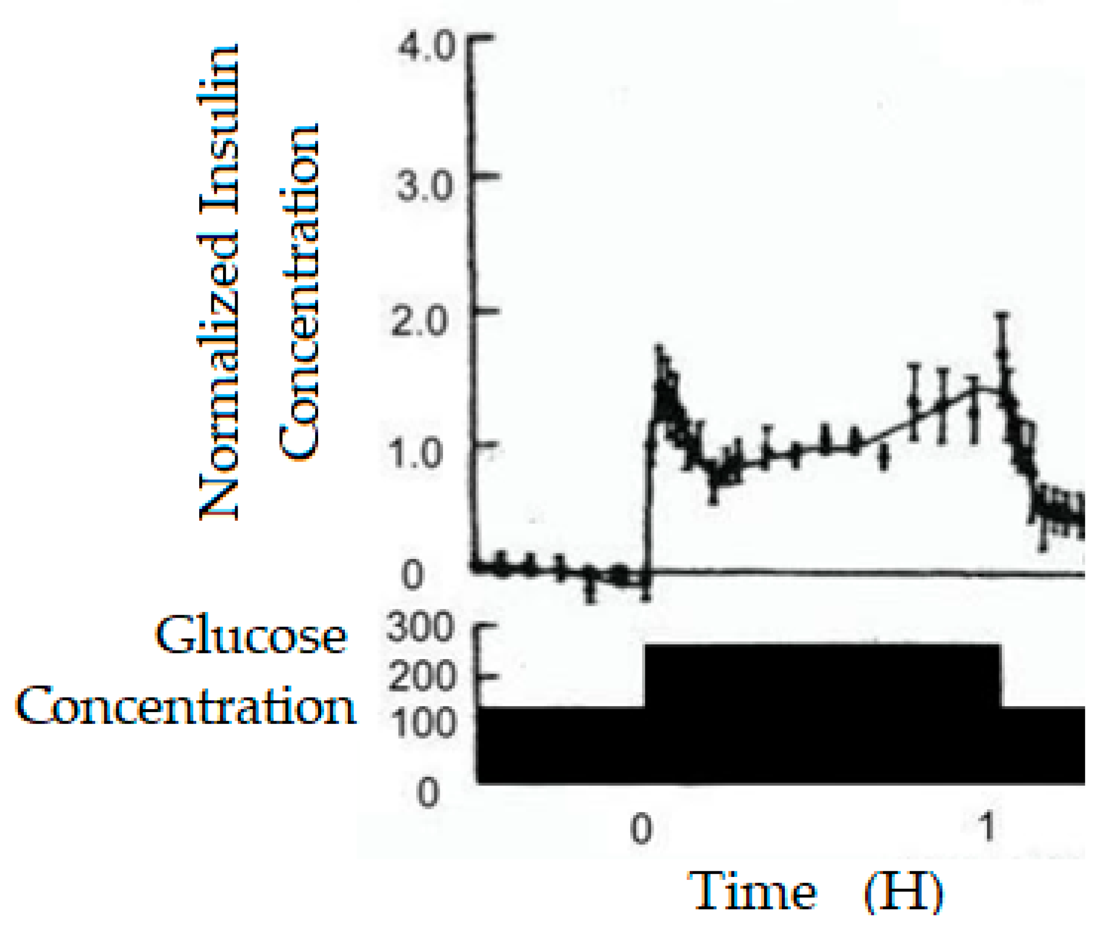
Figure 3.
On the right, the Insulin concentration response obtained from the Fisher model as response to the step increase of blood glucose concentration on the left.
Figure 3.
On the right, the Insulin concentration response obtained from the Fisher model as response to the step increase of blood glucose concentration on the left.
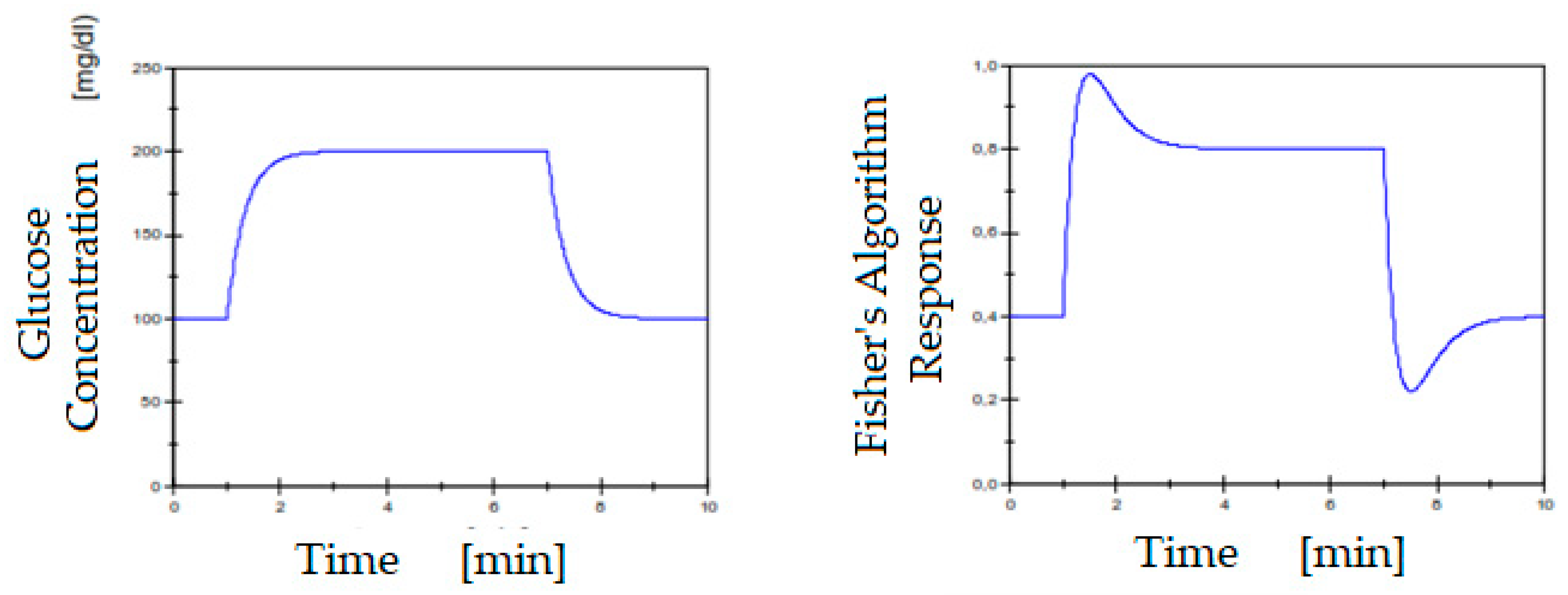
Figure 4.
Inflation dynamics following interest rate increase.
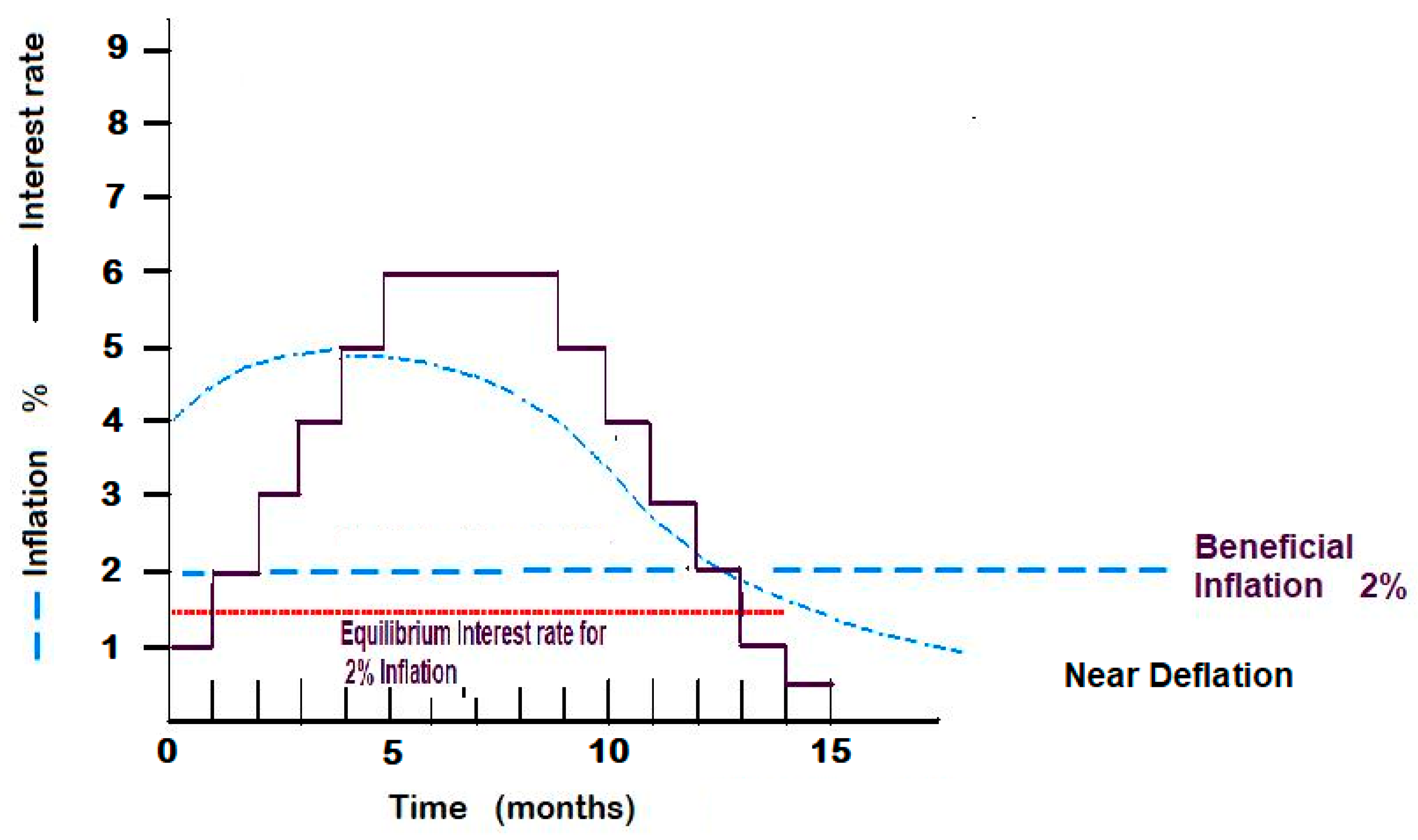
Disclaimer/Publisher’s Note: The statements, opinions and data contained in all publications are solely those of the individual author(s) and contributor(s) and not of MDPI and/or the editor(s). MDPI and/or the editor(s) disclaim responsibility for any injury to people or property resulting from any ideas, methods, instructions or products referred to in the content. |
© 2024 by the authors. Licensee MDPI, Basel, Switzerland. This article is an open access article distributed under the terms and conditions of the Creative Commons Attribution (CC BY) license (http://creativecommons.org/licenses/by/4.0/).
Copyright: This open access article is published under a Creative Commons CC BY 4.0 license, which permit the free download, distribution, and reuse, provided that the author and preprint are cited in any reuse.


