Submitted:
17 November 2024
Posted:
19 November 2024
Read the latest preprint version here
Abstract
In this paper we propose new entropy of the apparent horizon $S_h=(1/\beta)\arctan(\beta S_{BH})$, where $S_{BH}$ is the Bekenstein--Hawking entropy. As parameter $\beta\rightarrow 0$ one comes to the Bekenstein--Hawking entropy. This allows us to consider the generalised Friedmann--Lema\^{i}tre--Robertson--Walker (FLRW) equations for the barotropic matter fluid with $p=w\rho$ for arbitrary equation of state parameter $w$. We obtain the matter pressure $p$ and density energy $\rho$ corresponding to the apparent horizon. The modified Friedmann's equations are found. The addition term in the second modified Friedmann's equation plays the role of a dynamical cosmological constant. The dark energy density, pressure and the deceleration parameter are found. It was shown that at some parameters $w$ and $\beta$ we can have two phases, acceleration and deceleration or the eternal inflation. The model under consideration by using the holographic principle describes the universe inflation. Thus, we consider the holographic dark energy model with the generalised entropy of the apparent horizon. New cosmology based on the generalized entropy can be of interest for a description of inflation and late time of the universe evolution.
Keywords:
entropy
; apparent horizon
; Friedmann's equations
; barotropic matter fluid
; dynamical cosmological constant
; dark energy
; deceleration parameter
; cosmology based on the generalized entropy can be of interest for a description of inflation and late time of the universe evolution
1. Introduction
It was proven that black holes obey thermodynamic laws where entropy is proportional to the horizon area [1,2] and temperature is connected with the surface gravity so that gravity is related to ordinary thermodynamics [3,4,5,6]. The Friedmann equations also can be obtained from the first law of apparent horizon thermodynamics [7,8,9,10,11,12,13,14,15,16,17]. Different forms of entropies were considered which lead to modified Friedmann’s equations [18,19,20,21,22,23,24,25]. Entropies are sources of holographic energy densities that can describe the dark energy of the universe [26,27]. Here, we propose new apparent horizon entropy with being the Bekenstein–Hawking entropy. Our entropy, as well as other viable entropies, vanishes when the Bekenstein–Hawking entropy becomes zero. In addition, the entropy under consideration is the monotonically increasing function of the Bekenstein–Hawking entropy and is positive which is the natural requirement. When parameter we have the Bekenstein–Hawking entropy, . It is worth mentioning that the apparent horizon thermodynamics leads to the Friedmann equations within Einstein’s gravity only for a particular case when the matter is a perfect fluid with equation of state (EoS) given by , where p is the matter pressure and is the density energy of matter [16]. Here, we modify the Bekenstein–Hawking entropy by apparent horizon entropy to consider the general case with arbitrary EoS state parameter for barotropic perfect fluid including the case . It is known that the long-range gravitational interactions are better described by generalized entropies.
We will show that our entropy results to modified Friedmann’s equations and the universe inflation. This approach corresponds to Einstein’s equations with dynamical cosmological constant. As a result, the universe inflation and dark energy are due to dynamical cosmological constant. It is worth mentioning that the inflation of the universe can be explained, for example, by coupling Einstein’s gravity with nonlinear electrodynamics (see [28] and references therein).
2. Thermodynamics of Apparent Horizon
In the following we consider the FLRW flat universe with the metric
where is a scale factor and denotes the line element of an 2-dimensional unit sphere. For the FLRW universe the radius of the apparent horizon reads
with the Hubble parameter of the universe , where dot over means the derivative with respect to the cosmological time t. The total energy inside the space is
while is the change of the energy inside the apparent horizon. Here, denotes the energy density of matter fields. The first law of apparent horizon thermodynamics is given by
where the work density in the cosmology is
where p being the matter pressure. The apparent horizon temperature is given by
From first law of apparent horizon thermodynamics (2.4), taking into account equations (2.2), (2.3) and (2.5), we obtain
or
where we have used the continuity equation (the energy momentum conservation)
3. Modified FLRW Equations
From Eqs. (2.7) and (2.8) we obtain
From our proposed entropy
with , one finds from Eq. (3.1) the modified Friedmann equation
At equation (3.3) becomes the usual Friedmann equation for flat universe within general relativity. Utilizing Eq. (2.8) and after integrating Eq. (3.3), we obtain the second modified Friedmann equation
At we comes to usual FLRW equation for flat universe within Einstein’s gravity. Equation (3.4) can be represented as
where plays the role of the effective (a dynamical) cosmological constant. From Eq. (3.5) we obtain the dark energy density
At small the effective cosmological constant becomes while at small it reads . The plot of versus H at different is given in Figure 1.
Implying that dark substance obeys ordinary conservation law, where no mutual interaction between the cosmos components, we find the pressure
Making use of Eqs. (3.6) and (3.7) one finds the pressure
The second law of thermodynamics leads to the requirement and from Eq. (3.2) we obtain or . Thus, we have the same inequality as for the Bekenstein–Hawking entropy. This requirement for positive Hubble parameter gives . As a result, from Eq. (3.3) one finds or for positive energy density we have for EoS parameter . One can use the redshift instead of the scale factor , where is a constant corresponding to a scale factor at the current time. Then from the continuity equation (2.8) and EoS we find the density energy of matter as
where is the density energy of matter at the present time. Making use of Eqs. (3.4) and (3.9) we obtain
In Figure 2 we depicted the function of apparent horizon radius versus redshift z for , , .
As redshift increases the apparent horizon radius decreases.
The deceleration parameter is defined as
When the acceleration phase takes place but as we have the universe deceleration. By virtue of Eqs. (3.3), (3.9) and (3.11) we obtain
Equations (3.4), (3.9) and (3.12) define the function of the deceleration parameter q versus redshift z. Making use of Eqs. (3.4) and (3.12) one finds also the deceleration parameter q as a function of H at fixed and EoS parameter w
In Figure 3 we plotted the function of the deceleration parameter q versus the Hubble parameter H for , , .
For some parameters w and there are two eras: inflation and deceleration but in some w and we have only eternal university acceleration (inflation). From Eq. (3.13) we obtain the asymptotic
Thus, the asymptotic of the deceleration parameter does not depend on the entropy parameter . At we obtain from Eq. (3.13) that . Figure 3 is in accordance with the formula (3.14). Making use of Eq. (3.14), we obtain the condition when two phases, acceleration and deceleration, take place: (). When the eternal inflation is realised. With the help of Eq. (3.4) and (3.9) we obtain the redshift
The approximate real and positive solutions to Eq. (3.13) for the transition redshifts when , , are given in Table 1. Table I shows that when the entropy parameter increases the Hubble parameter H and reshift z also increase (at fixed w) for a divided point between two pases, universe acceleration and deceleration. One can calculate deceleration parameter q for matter dominated era () and for the current era (), from Eqs. (3.13) and (3.15). We obtain from Eq. (3.15) for the current era, when , solutions for the Habble parameter H and deceleration parameter q from Eq. (3.13) for different entropy parameters , presented in Table II. Negative value of the deceleration parameter q in Table II indicates on the acceleration phase in the current time. According to [30] the deceleration parameter at the current time is . Table II shows that there is entropy parameter which can produce that result. Making use of (3.15) we depicted the dependence of Habble parameter H on redshift z in Figure 4.
According to Figure 4, when z increases, H also increases. At fixed , if EoS parameter w increases the Habble parameter H also increases. In accordance with figure, if parameter increases at fixed w the Habble parameter H also increases. With the help of Eqs. (3.13) and (3.15) we plotted the deceleration parameter q versus redshift z in Figure 5.
According to Figure 5, when z increases q also increases. At fixed (Left panel), if EoS parameter w increases the deceleration parameter q also increases. At and there are two phases, acceleration and deceleration but at one has only the acceleration phase (eternal inflation). In accordance with Figure 5 (Right panel), if parameter increases at fixed w the deceleration parameter q also increases. Here we have two phases: acceleration and deceleration.
4. Summary
Thus, we have proposed entropy which shares similar property as the Bekenstein–Hawking entropy : it vanishes when the apparent horizon radius vanishes; monotonically increases as the apparent horizon radius increases and it is positive. We consider the barotropic perfect fluid and flat FLRW universe. From first law of apparent horizon thermodynamics we obtained the modified Friedmann’s equations. The addition term in the second Friedmann’s equation is treated as a dynamical cosmological constant. We showed that the universe inflation is due to holographic dark energy. It is worth noting that Barrow’s and Tsallis’s entropies also lead to Einsten’s equations with the dynamical cosmological constant [29]. By analysing the deceleration parameter we find that for some parameters our model can describe inflation and deceleration phases or only eternal inflation. We have calculated the transition redshifts when , presented in Table I for some parameters w and . Table II shows that at and we obtain the current deceleration parameter . Cosmology based on the modified Friedmann equations obtained may be of interest for a description of inflation and late time of the universe evolution.
References
- J. D. Bekenstein, Black Holes and Entropy, Phys. Rev. D 7 (1973), 2333-2346.
- S. W. Hawking, Particle creation by black holes, Commun. Math. Phys. 43 (1975), 199-220; Erratum: ibid. 46 (1976), 206.
- T. Jacobson, Thermodynamics of Spacetime: The Einstein Equation of State, Phys. Rev. Lett. 75 (1995), 1260.
- T. Padmanabhan, Gravity and the Thermodynamics of Horizons, Phys. Rept. 406 (2005), 49.
- T. Padmanabhan, Thermodynamical Aspects of Gravity: New insights, Rept. Prog. Phys. 73 (2010), 046901.
- S. A. Hayward, Unified first law of black-hole dynamics and relativistic thermodynamics, Class. Quant. Grav. 15 (1998), 3147-3162.
- M. Akbar and R. G. Cai, Thermodynamic Behavior of Friedmann Equation at Apparent Horizon of FRW Universe, Phys. Rev. D 75 (2007), 084003.
- R. G. Cai and L. M. Cao, Unified First Law and Thermodynamics of Apparent Horizon in FRW Universe, Phys. Rev. D 75 (2007), 064008.
- A. Paranjape, S. Sarkar and T. Padmanabhan, Thermodynamic route to Field equations in Lanczos-Lovelock Gravity, Phys. Rev. D 74 (2006), 104015.
- A. Sheykhi, B. Wang and R. G. Cai, Thermodynamical Properties of Apparent Horizon in Warped DGP Braneworld, Nucl. Phys. B 779, (2007) 1.
- R. G. Cai and N. Ohta, Horizon Thermodynamics and Gravitational Field Equations in Horava-Lifshitz Gravity, Phys. Rev. D 81 (2010), 084061.
- M. Jamil, E. N. Saridakis and M. R. Setare, The generalized second law of thermodynamics in Horava-Lifshitz cosmology, JCAP 1011 (2010), 032.
- Y. Gim, W. Kim and S. H. Yi, The first law of thermodynamics in Lifshitz black holes revisited, JHEP 1407 (2014), 002.
- Z. Y. Fan and H. Lu, Thermodynamical First Laws of Black Holes in Quadratically-Extended Gravities, Phys. Rev. D 91 (2015), 064009.
- R. D’Agostino, Holographic dark energy from nonadditive entropy: cosmological perturbations and observational constraints, Phys. Rev. D 99 (2019), 103524.
- L. M. Sanchez and H. Quevedo, Thermodynamics of the FLRW apparent horizon, Phys. Lett B 839 (2023), 137778.
- S. Wang, Y. Wang and M. Li, Holographic Dark Energy, Phys. Rept. 696 (2017) 1.
- C. Tsallis, Possible generalization of Boltzmann-Gibbs statistics, J. Stat. Phys., 52 (1-2) (1988), 479-487; C. Tsallis, The Nonadditive Entropy Sq and Its Applications in Physics and Elsewhere: Some Remarks, Entropy 13, 1765 (2011).
- J. Ren, Analytic critical points of charged Renyi entropies from hyperbolic black holes, JHEP 05 (2021), 080.
- A. R´enyi, Proceedings of the Fourth Berkeley Symposium on Mathematics, Statistics and Probability, University of California Press (1960), 547-56.
- A. Sayahian Jahromi et al, Generalized entropy formalism and a new holographic dark energy model, Phys. Lett. B 780 (2018), 21-24.
- J. D. Barrow, The Area of a Rough Black Hole, Phys. Lett. B 808 (2020), 135643.
- G. Kaniadakis, Statistical mechanics in the context of special relativity II, Phys. Rev. E 72 (2005), 036108.
- K. Mejrhit and S. E. Ennadifi, Thermodynamics, stability and Hawking–Page transition of black holes from non-extensive statistical mechanics in quantum geometry, Phys. Lett. B 794 (2019), 45-49.
- S. Nojiri, S. D. Odintsov and Tanmoy Paul, Different aspects of entropic cosmology, Phys. Lett. B 835 (2022), 137553.
- D. Pavon and W. Zimdahl, Holographic dark energy and cosmic coincidence, Phys. Lett. B 628 (2005) 206.
- R. C. G. Landim, Holographic dark energy from minimal supergravity, Int. J. Mod. Phys. D 25 (2016), 1650050.
- S. I. Kruglov, Universe inflation and nonlinear electrodynamics, Eur. Phys. J. C 84 (2024), 205.
- Sofia Di Gennaro, Hao Xu, Yen Chin Ong, How barrow entropy modifies gravity: with comments on Tsallis entropy, Eur. Phys. J. C 82 (2022), 1066.
- M. Roos, Introduction to Cosmology (John Wiley and Sons, UK, 2003).
Figure 1.
The function versus H at . Figure 1 shows that increases as b increases. The asymptotic of effective cosmological constant is as .
Figure 1.
The function versus H at . Figure 1 shows that increases as b increases. The asymptotic of effective cosmological constant is as .
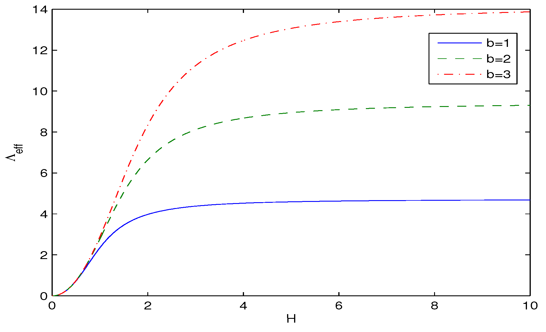
Figure 2.
Left panel: The function versus z at , , , , . Figure 2 shows that decreases as z increases. At fixed , when EoS parameter w increases the redshift z decreases. Right panel: According to figure the dependance of the apparent horizon radius on is very weak.
Figure 2.
Left panel: The function versus z at , , , , . Figure 2 shows that decreases as z increases. At fixed , when EoS parameter w increases the redshift z decreases. Right panel: According to figure the dependance of the apparent horizon radius on is very weak.
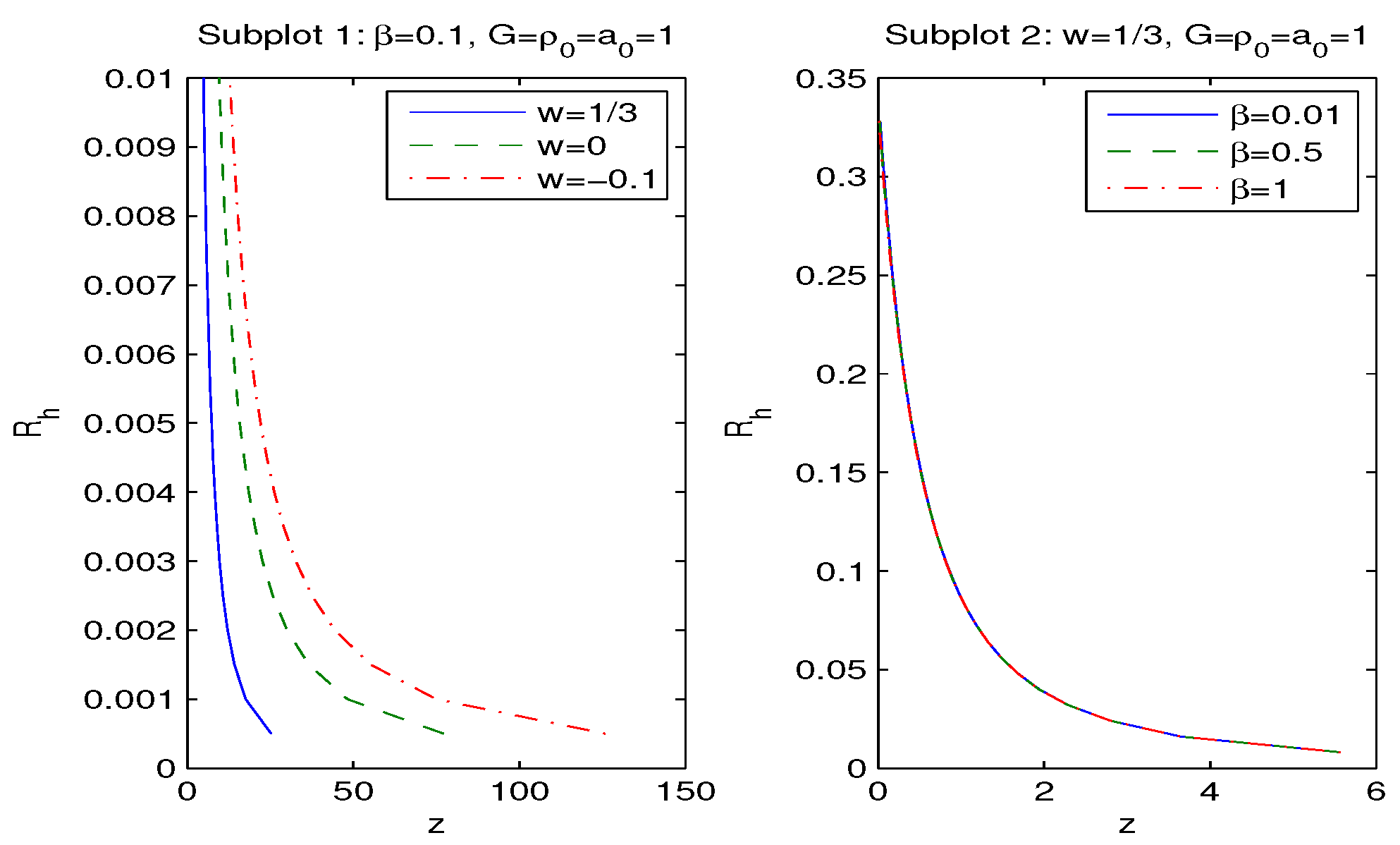
Figure 3.
Left panel: The function q versus H at , , -0.5, , , . Figure 2 shows that q increases as H increases. At fixed and H, when EoS parameter w increases the deceleration parameter q also increases. At and there are two phases, acceleration and deceleration but at one has only the acceleration phase (eternal inflation). Right panel: According to figure, if parameter increases at fixed w and H the deceleration parameter q also increases. Here we have two phases: acceleration and deceleration.
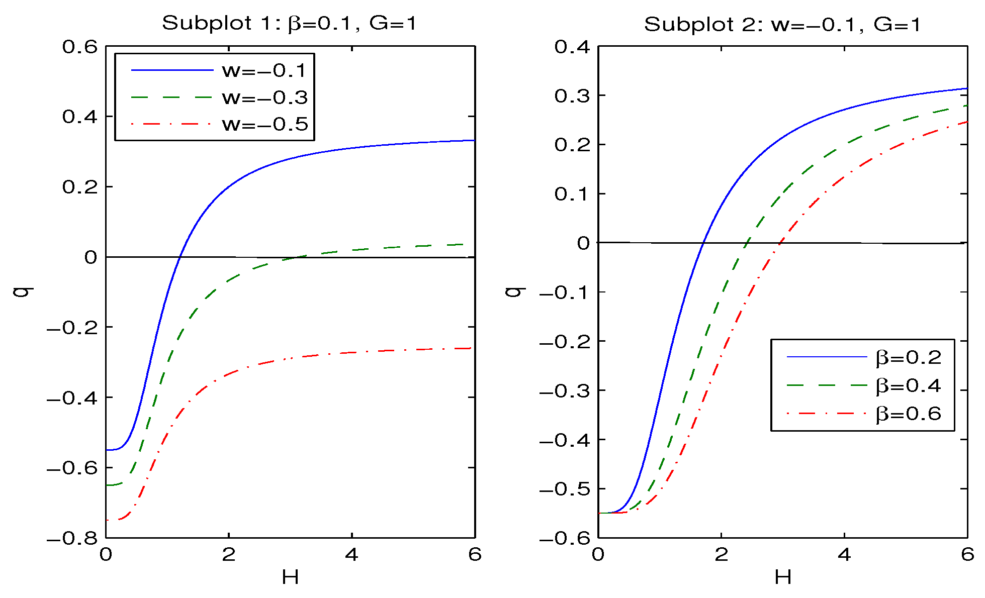
Figure 4.
Left panel: The function H versus z at , , -0.5, , . According to Figure 4, when z increases, H also increases. At fixed , if EoS parameter w increases the Habble parameter H also increases. Right panel: In accordance with figure, if parameter increases at fixed w the Habble parameter H also increases.
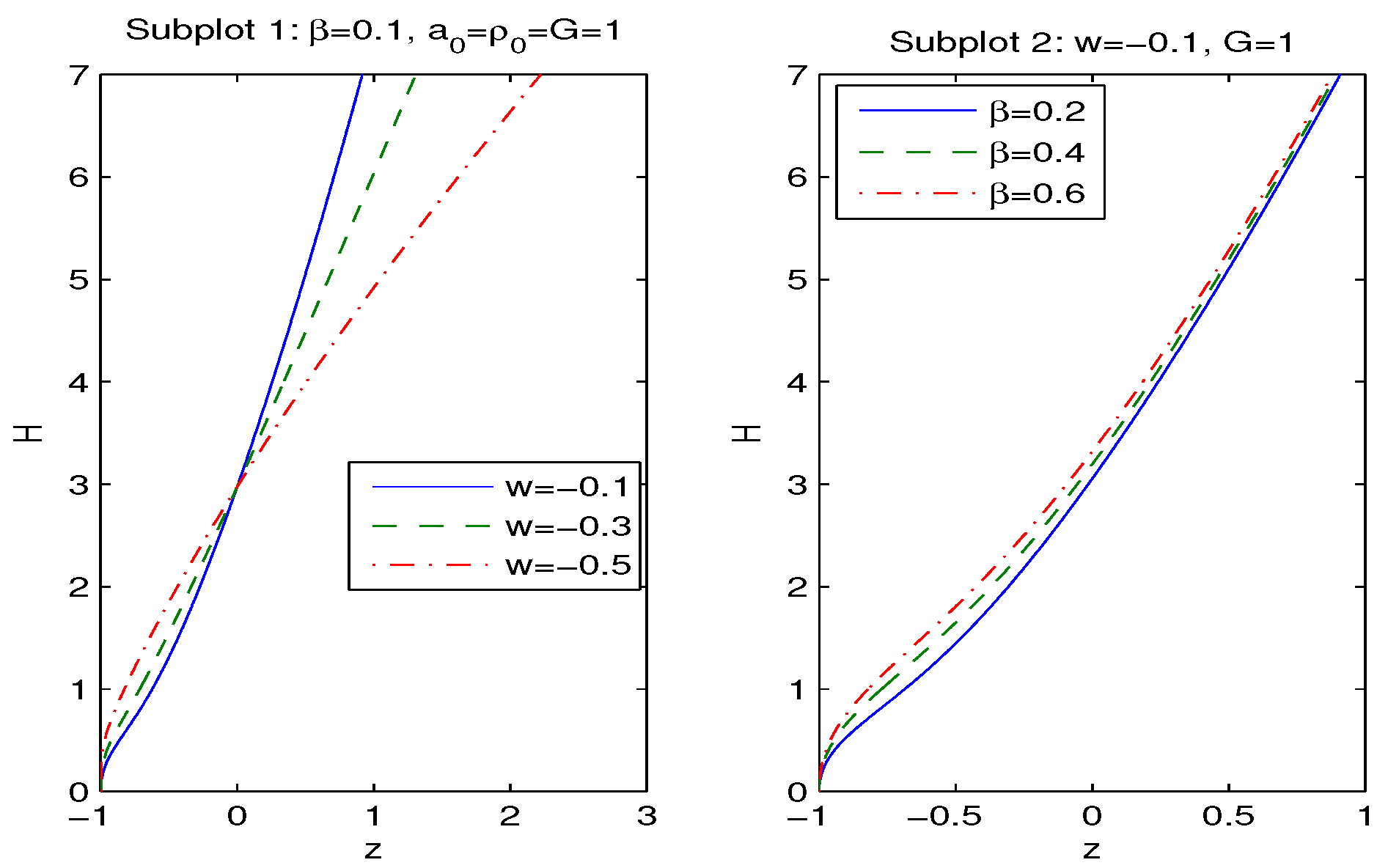
Figure 5.
Left panel: The function q versus z at , , -0.5, , . According to Figure 5, when z increases q also increases. At fixed , if EoS parameter w increases the deceleration parameter q also increases. At and there are two phases, acceleration and deceleration but at one has only the acceleration phase (eternal inflation). Right panel: In accordance with figure, if parameter increases at fixed w the deceleration parameter q also increases. Here we have two phases: acceleration and deceleration.
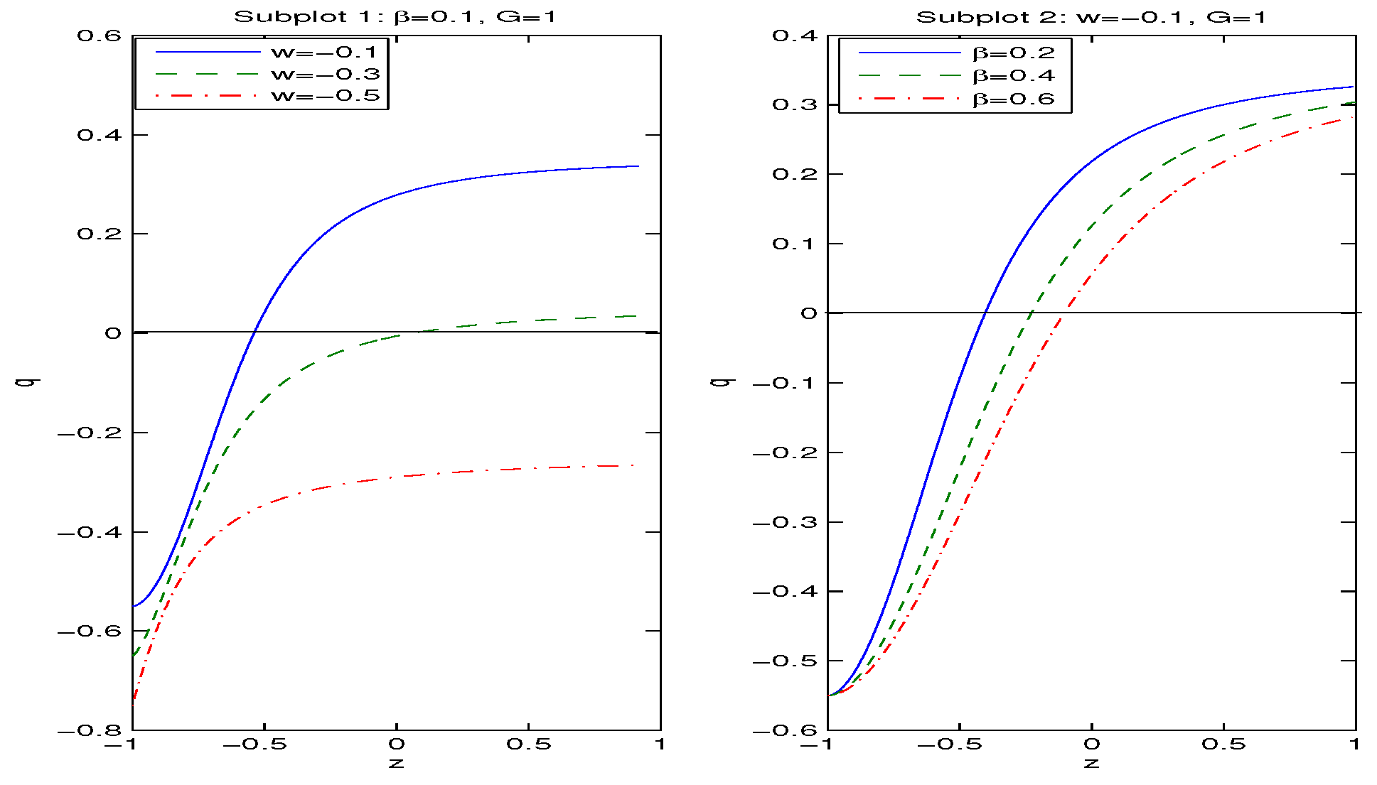

Table 1.
The approximate solutions to Eqs. (3.13) and (3.15) for the transition redshifts at , , .
| 0.7 | 0.8 | 0.9 | 1 | 1.1 | 1.2 | 1.3 | 1.4 | 1.5 | 1.6 | 1.7 | |
| H | 3.20 | 3.42 | 3.63 | 3.82 | 4.01 | 4.19 | 4.36 | 4.53 | 4.68 | 4.84 | 4.99 |
| -0.05 | -0.004 | 0.04 | 0.08 | 0.12 | 0.16 | 0.19 | 0.23 | 0.26 | 0.29 | 0.32 |
Table 2.
The approximate solutions to Eqs. (3.13) and (3.15) for the current era at , , .
| 0.1 | 0.2 | 0.3 | 0.4 | 0.5 | 0.6 | 0.7 | 0.8 | 0.9 | |
| H | 2.977 | 3.053 | 3.125 | 3.193 | 3.258 | 3.320 | 3.378 | 3.435 | 3.489 |
| 0.527 | 0.549 | 0.567 | 0.583 | 0.597 | 0.609 | 0.619 | 0.629 | 0.637 |
Disclaimer/Publisher’s Note: The statements, opinions and data contained in all publications are solely those of the individual author(s) and contributor(s) and not of MDPI and/or the editor(s). MDPI and/or the editor(s) disclaim responsibility for any injury to people or property resulting from any ideas, methods, instructions or products referred to in the content. |
© 2024 by the authors. Licensee MDPI, Basel, Switzerland. This article is an open access article distributed under the terms and conditions of the Creative Commons Attribution (CC BY) license (http://creativecommons.org/licenses/by/4.0/).
Copyright: This open access article is published under a Creative Commons CC BY 4.0 license, which permit the free download, distribution, and reuse, provided that the author and preprint are cited in any reuse.


