Submitted:
22 November 2024
Posted:
25 November 2024
Read the latest preprint version here
Abstract
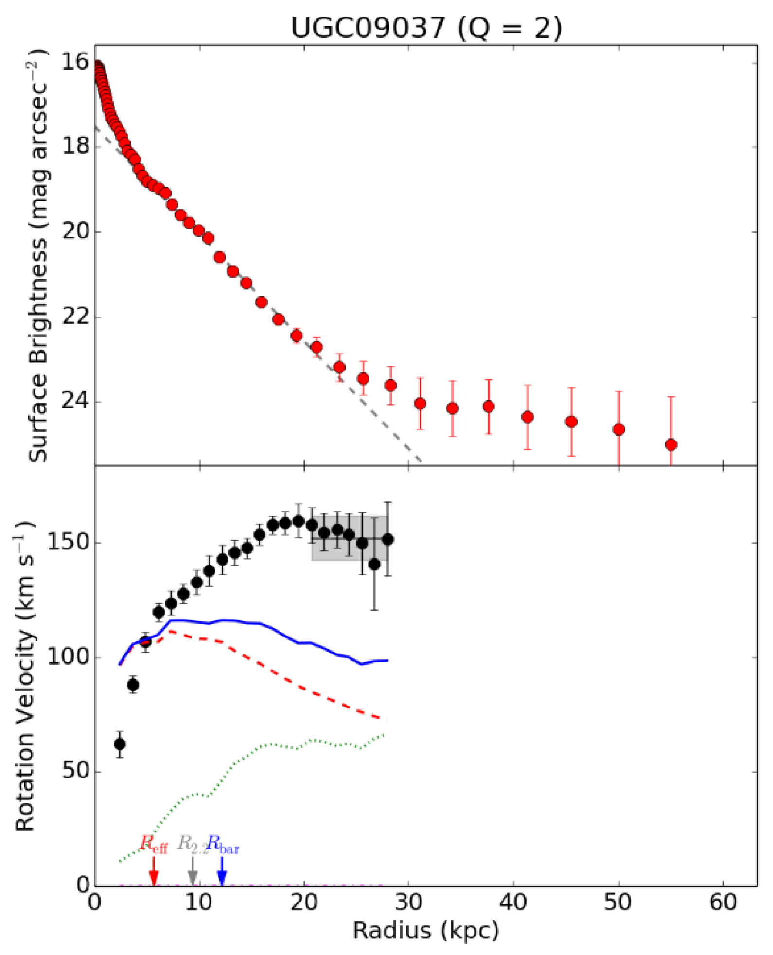
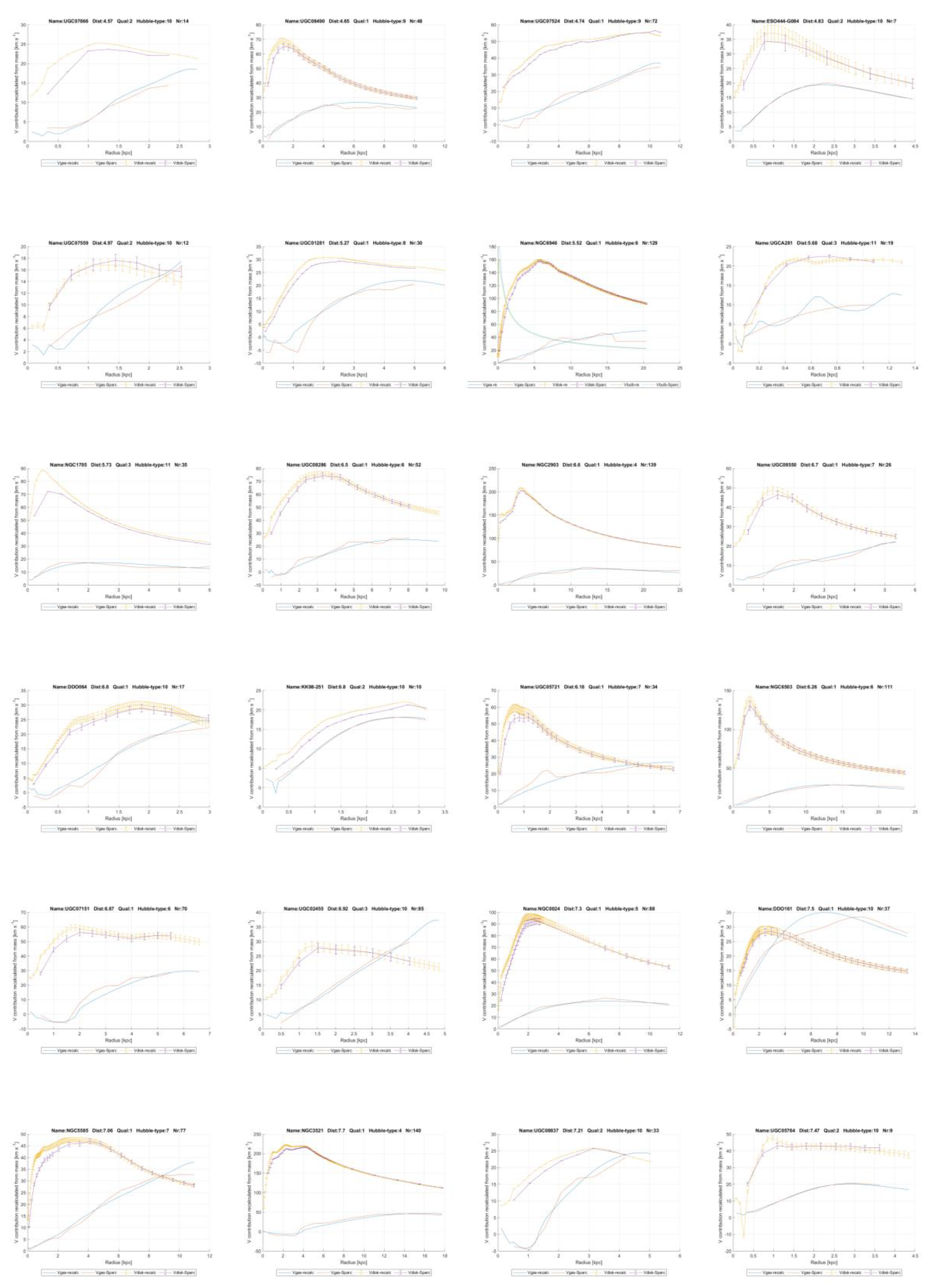
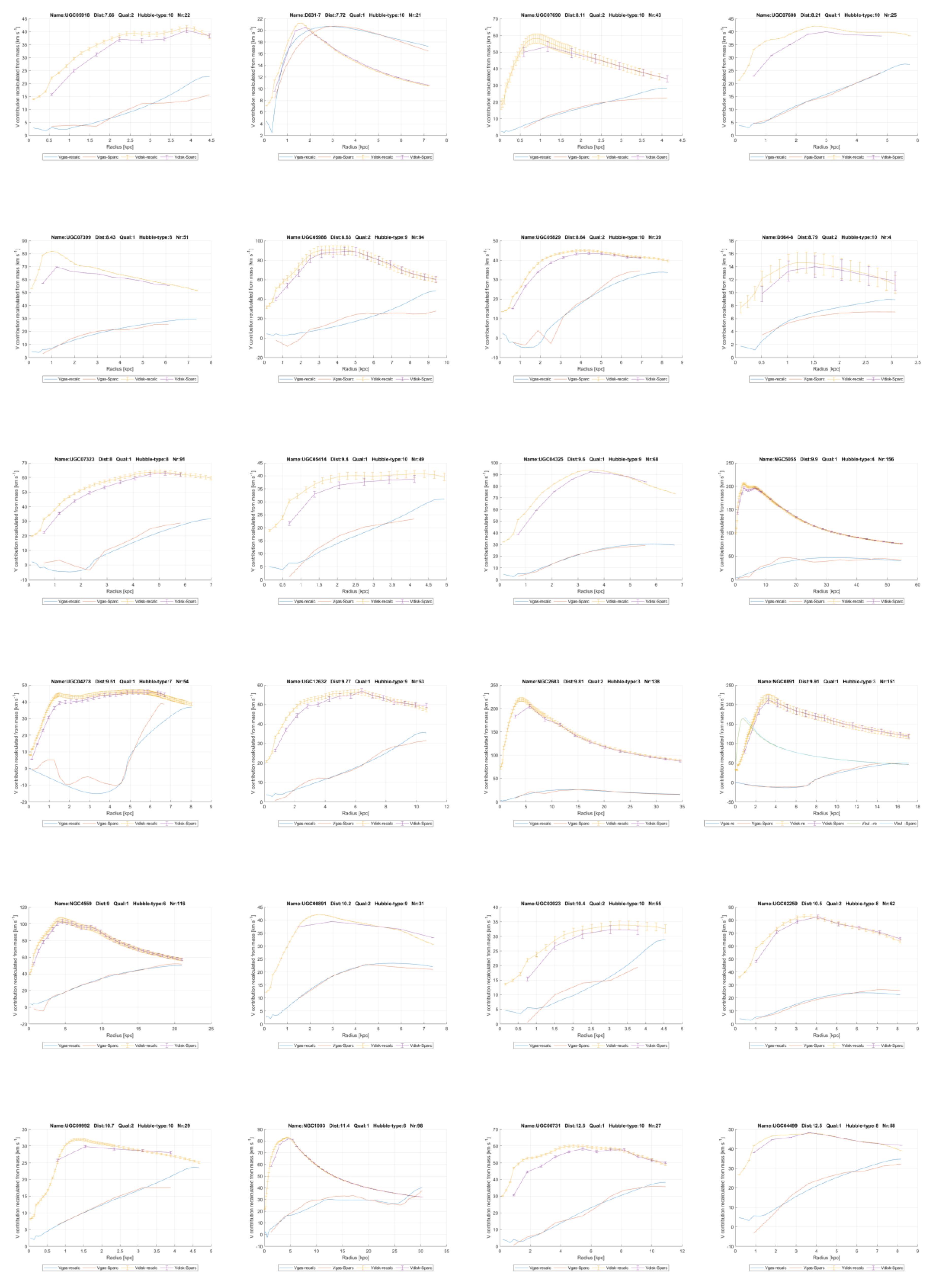
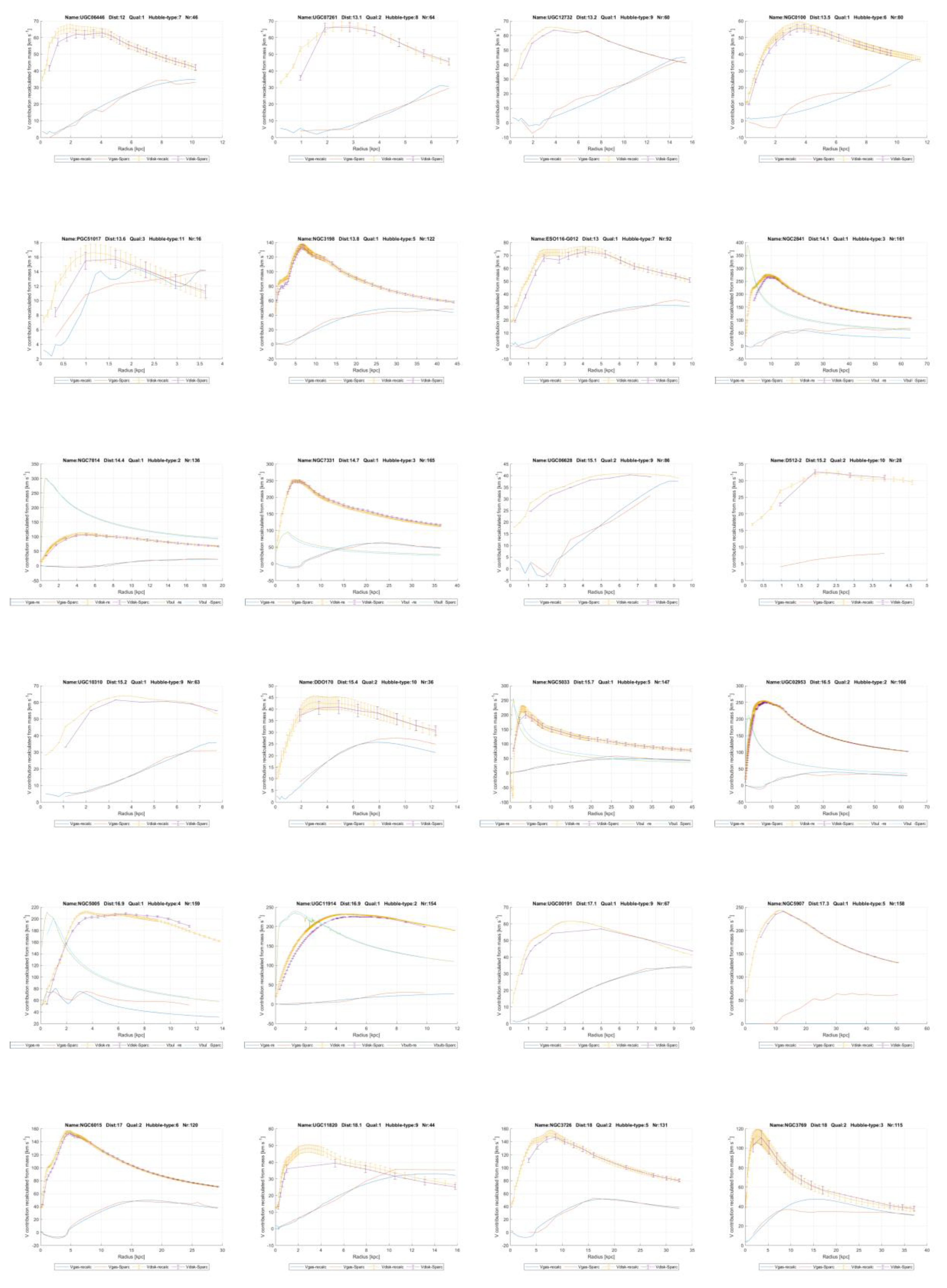
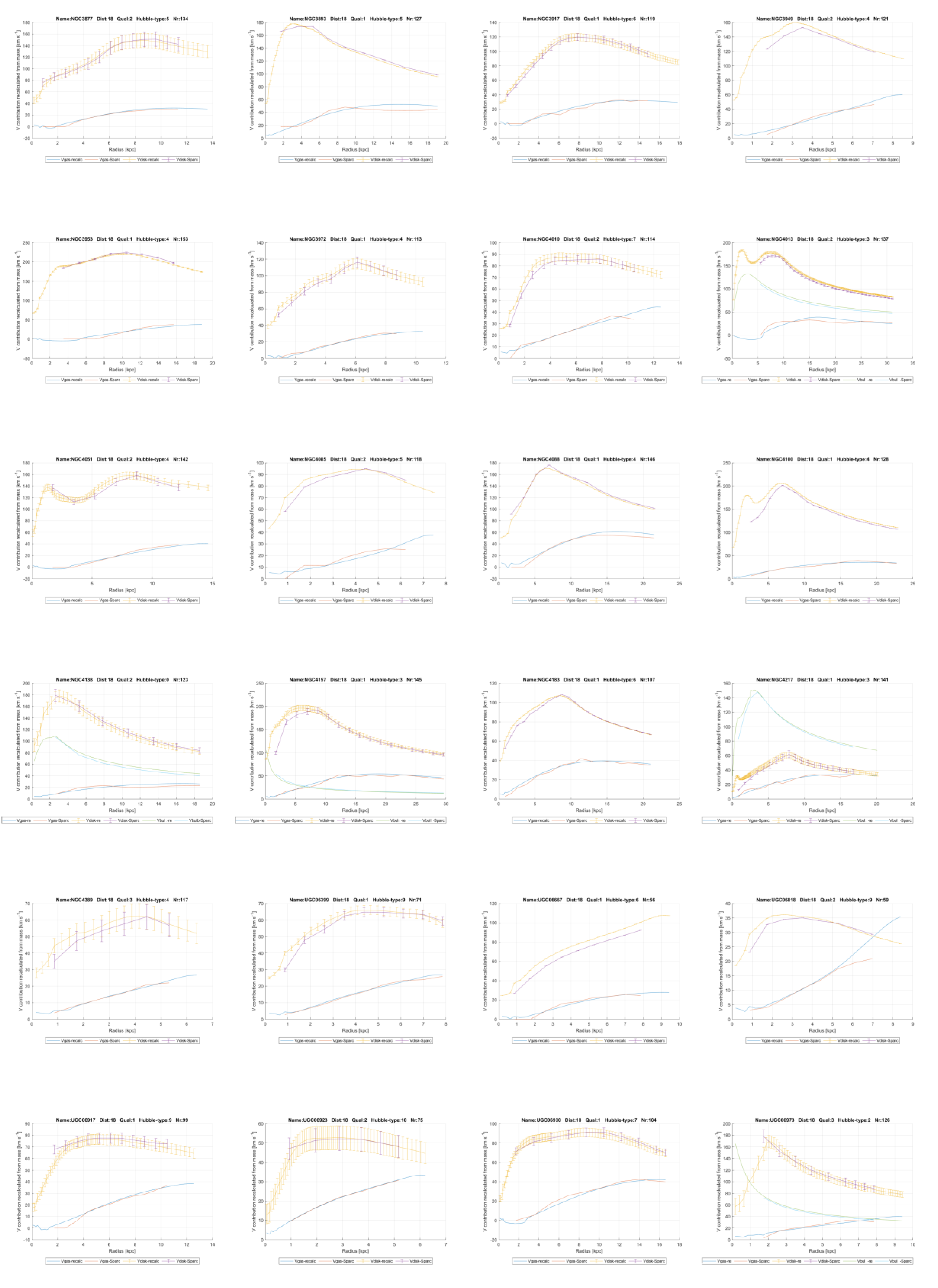
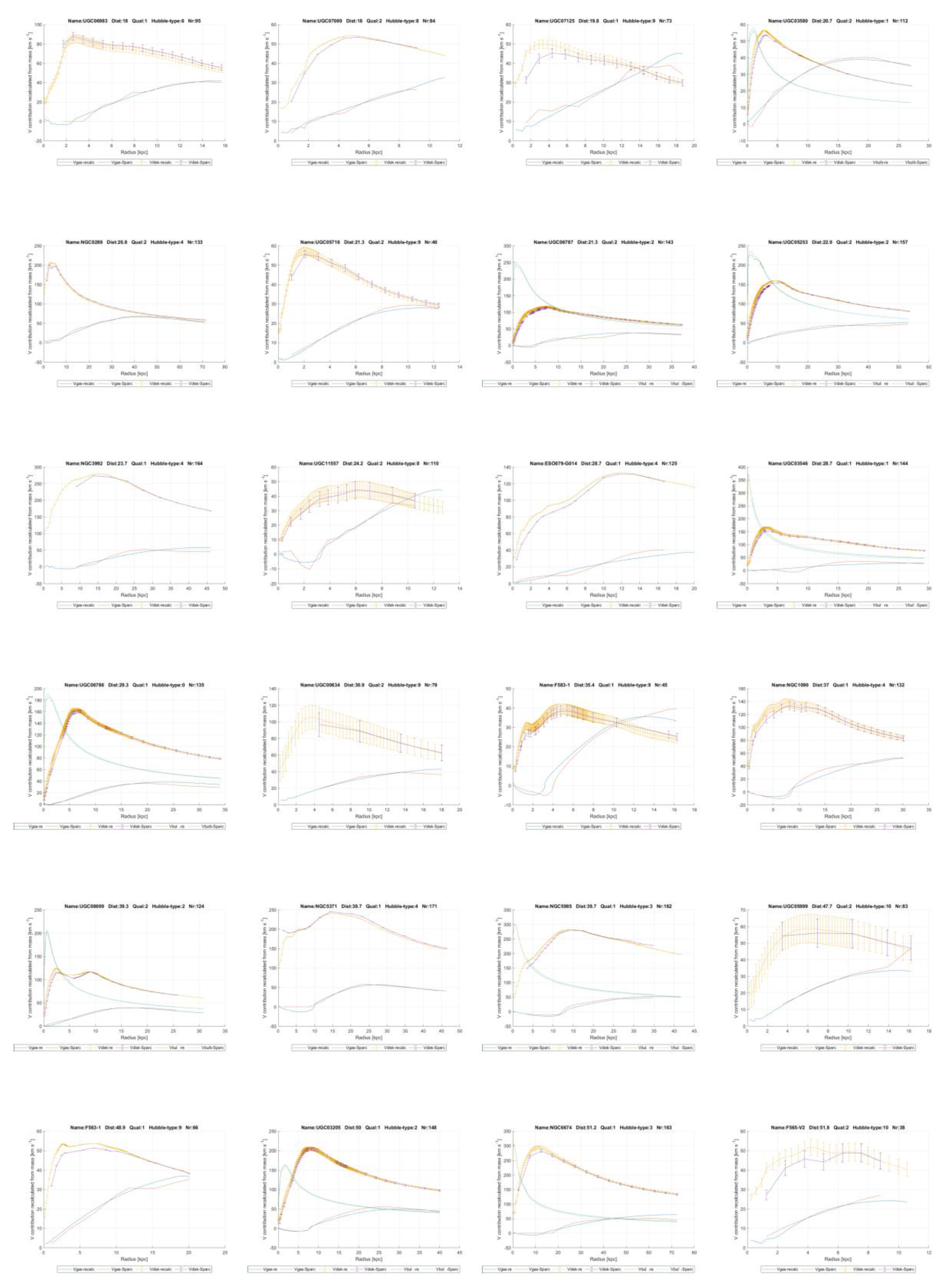
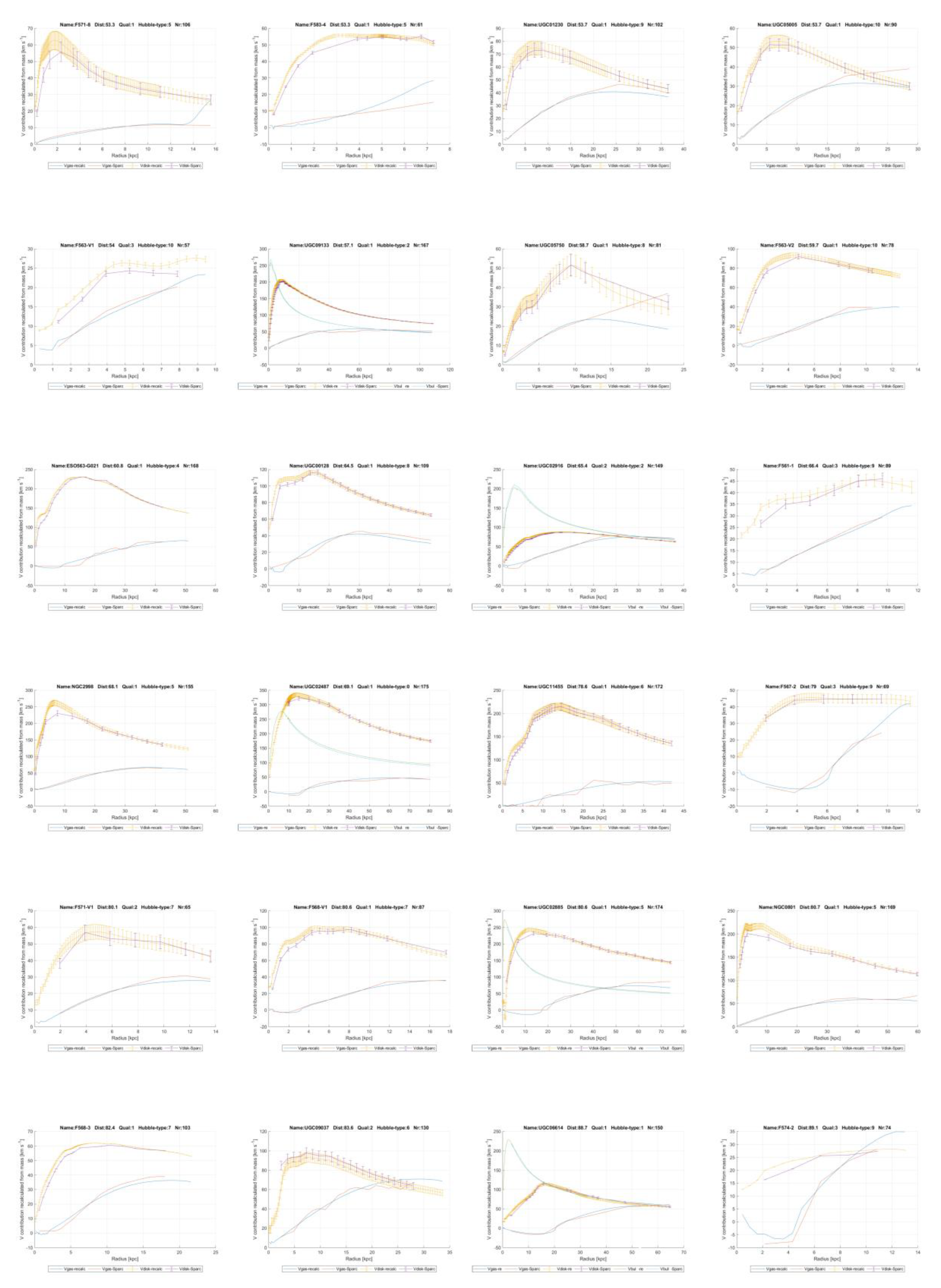
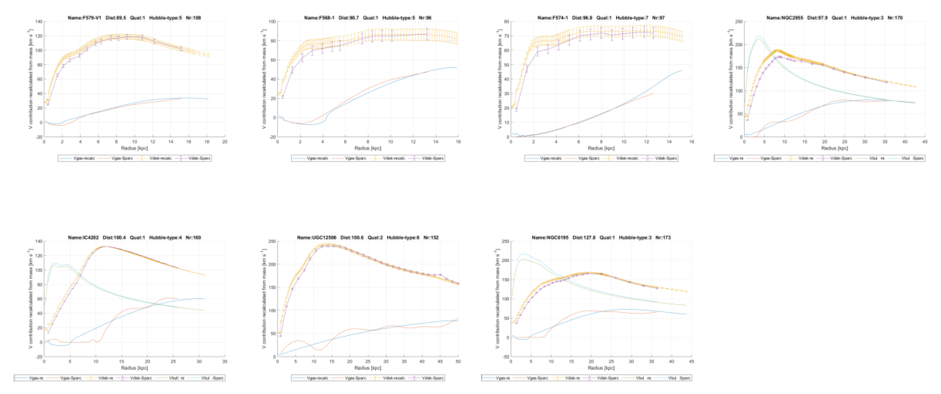
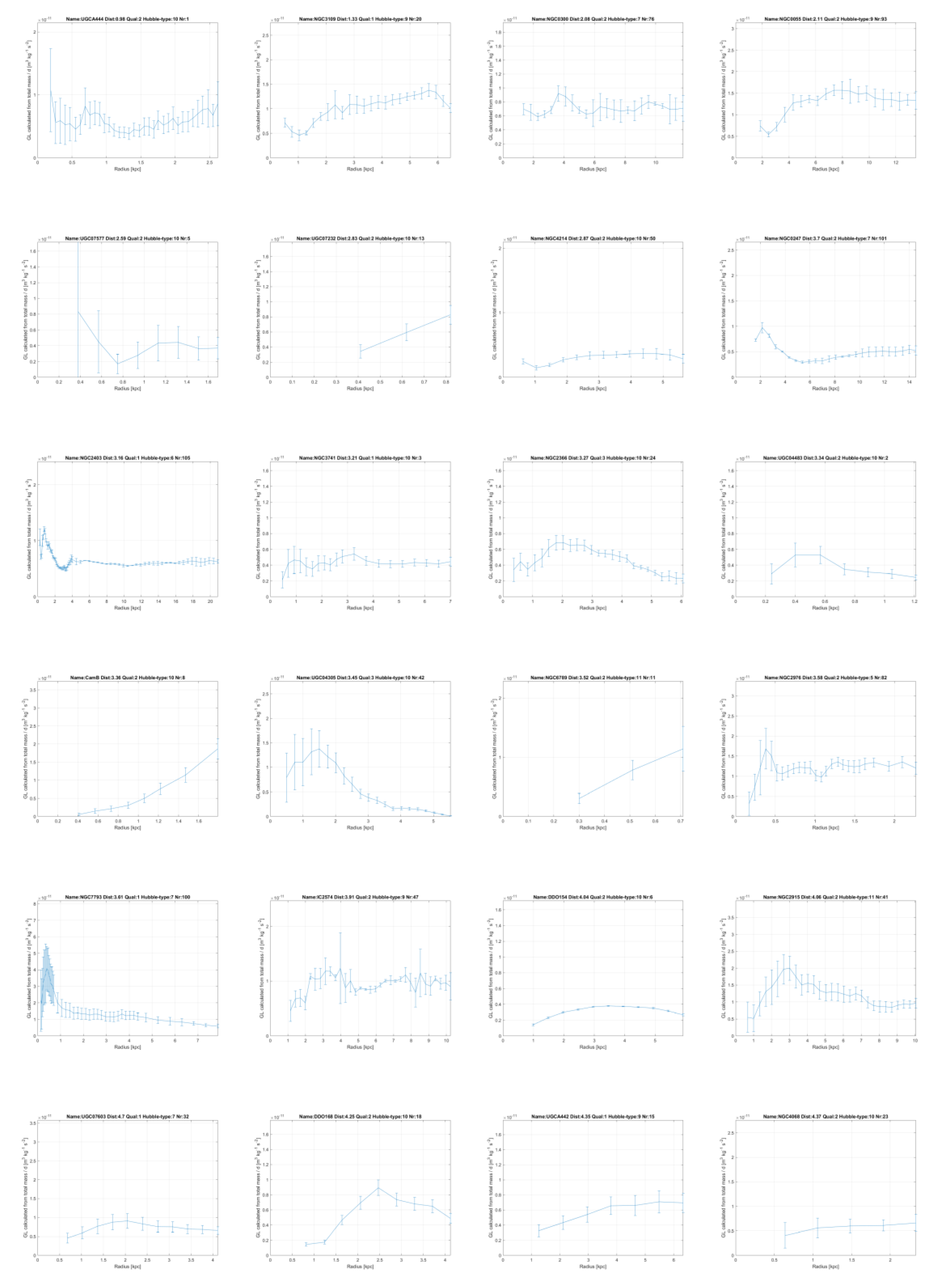
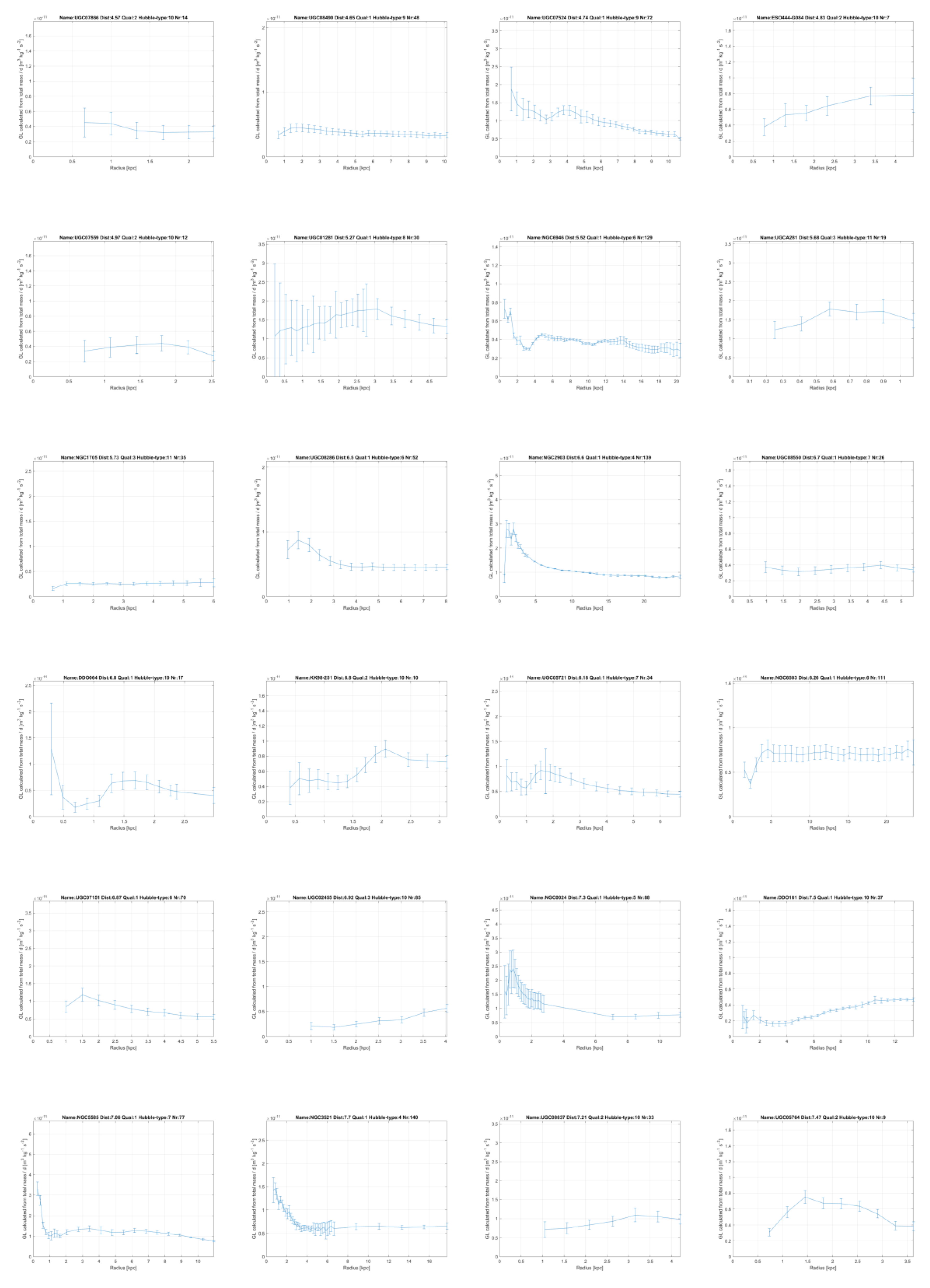
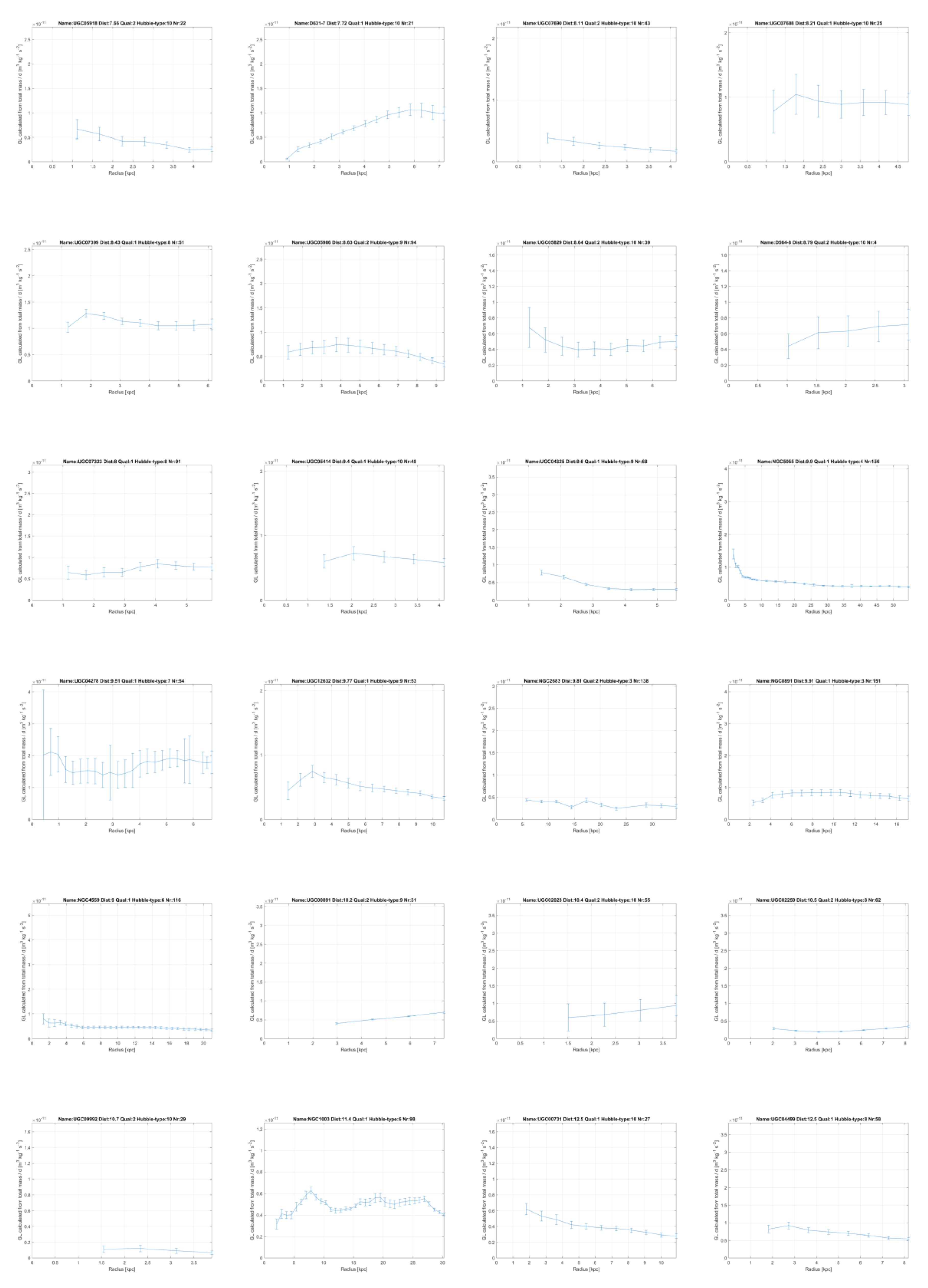
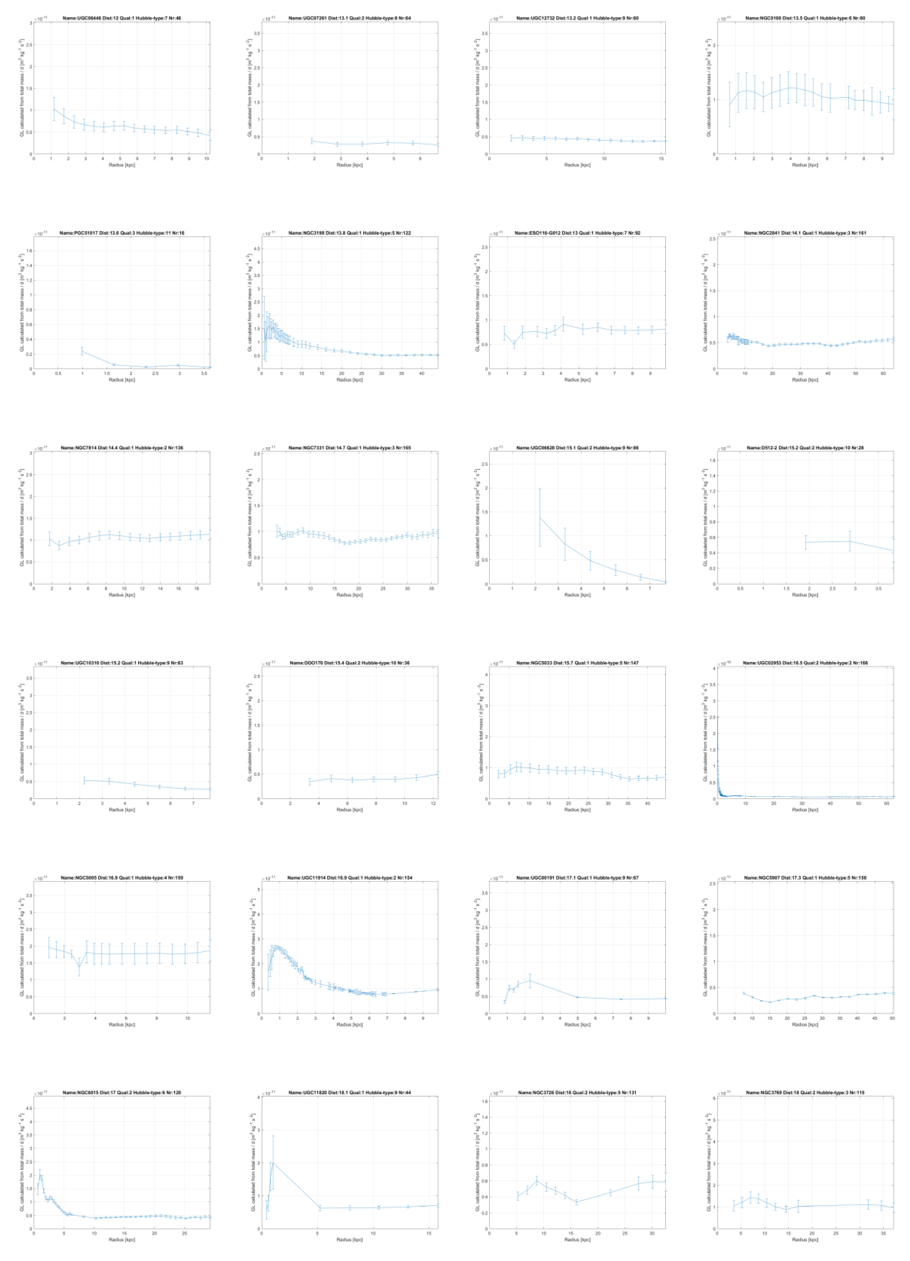
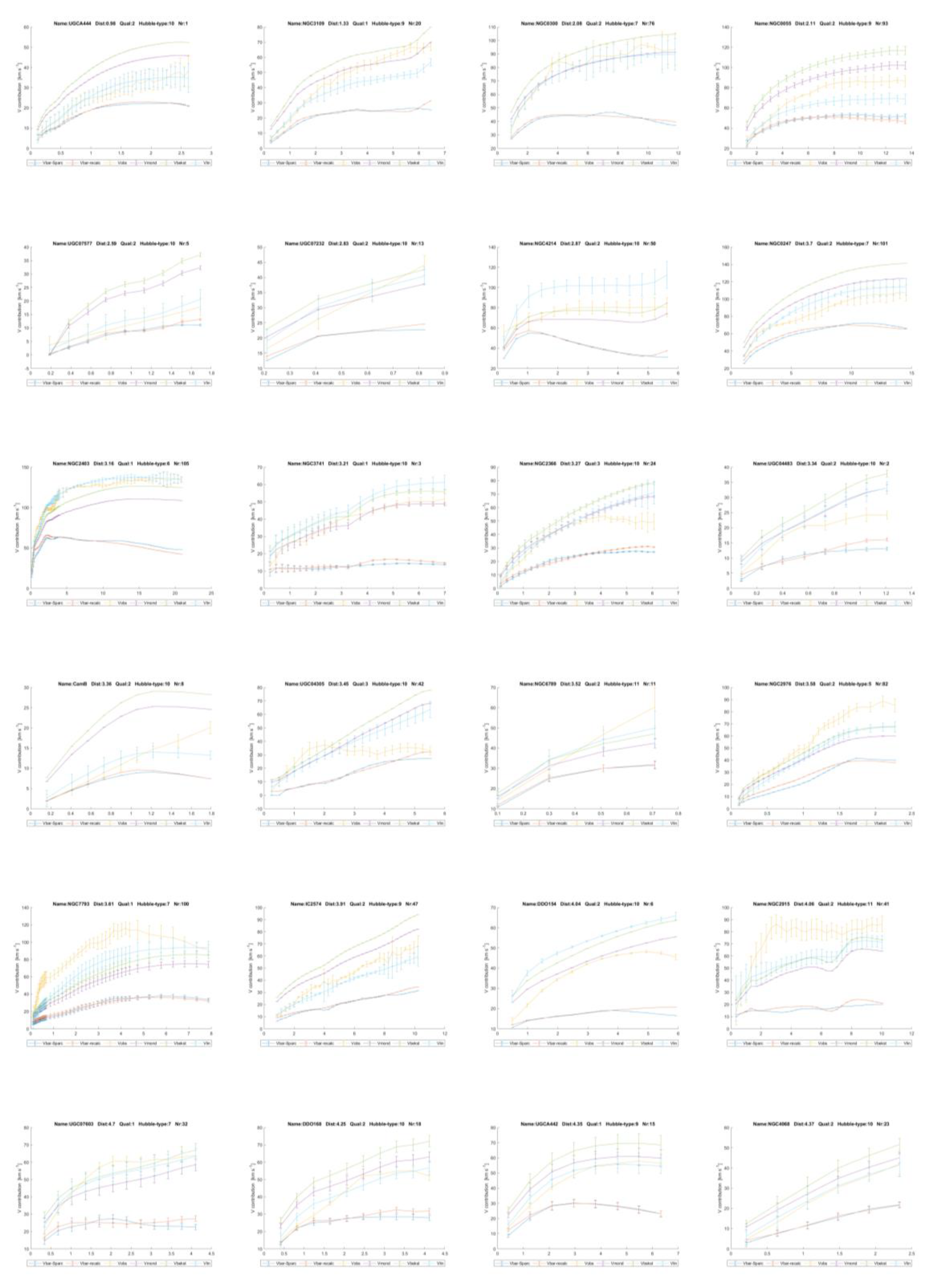
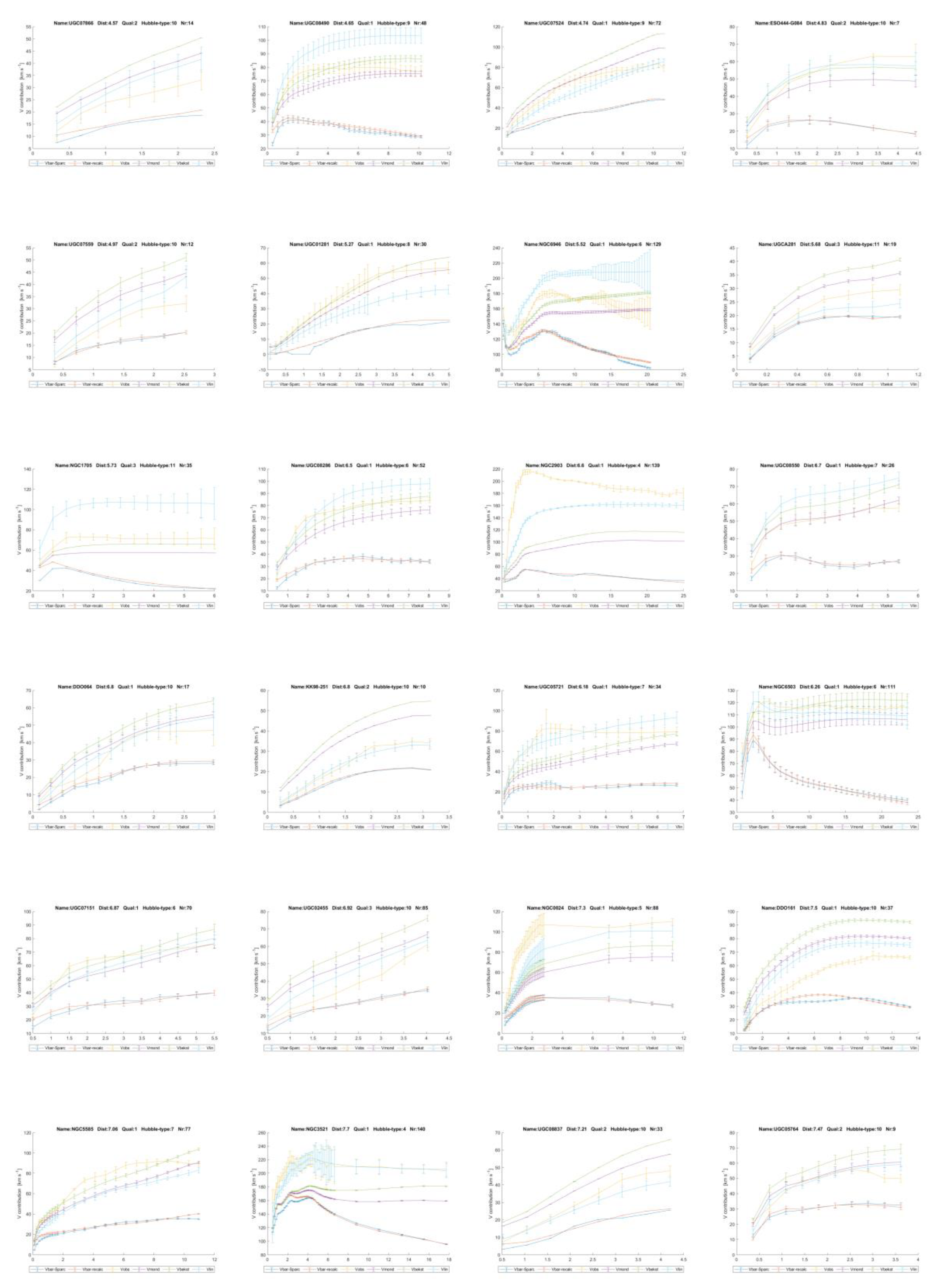
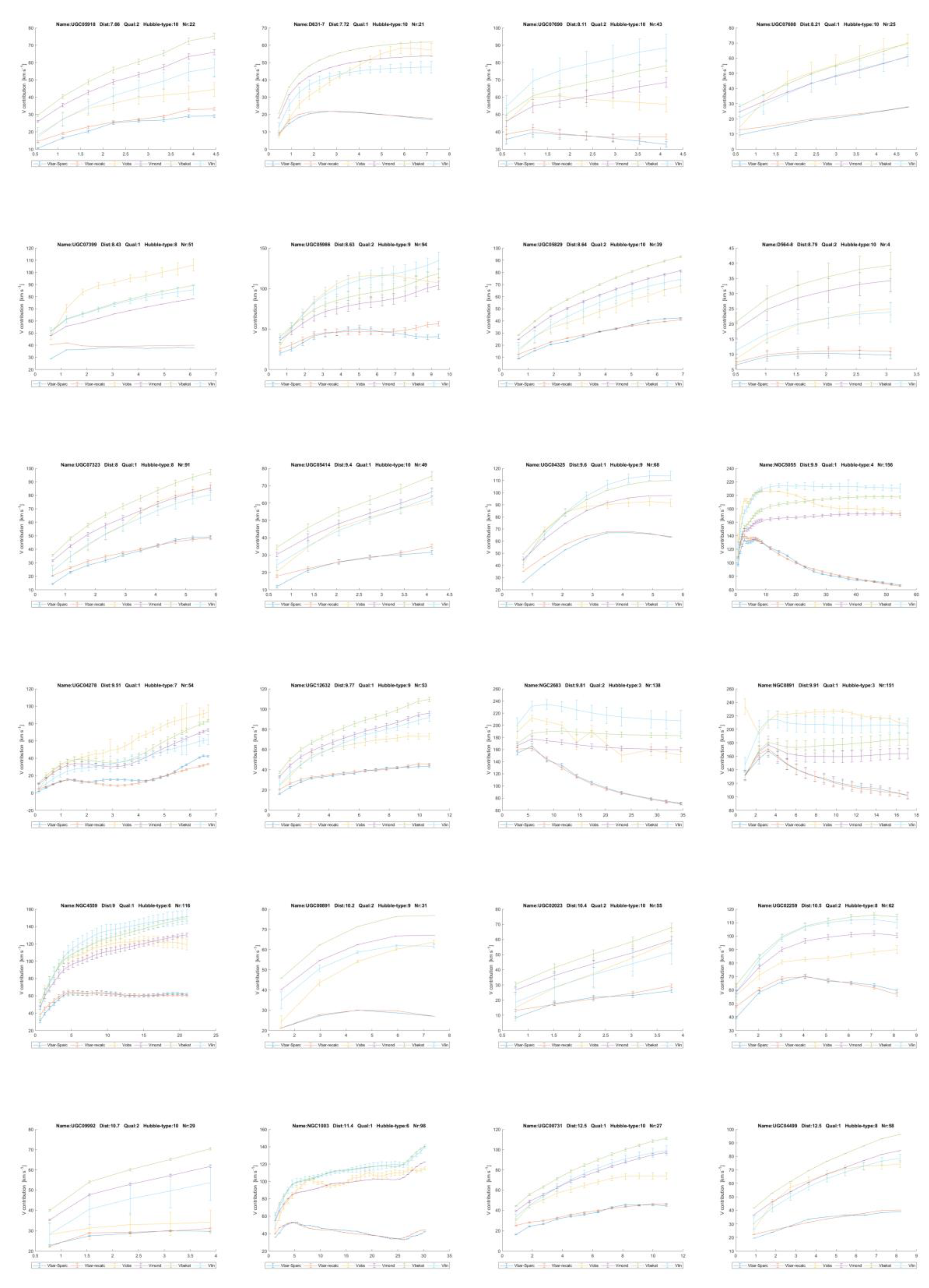
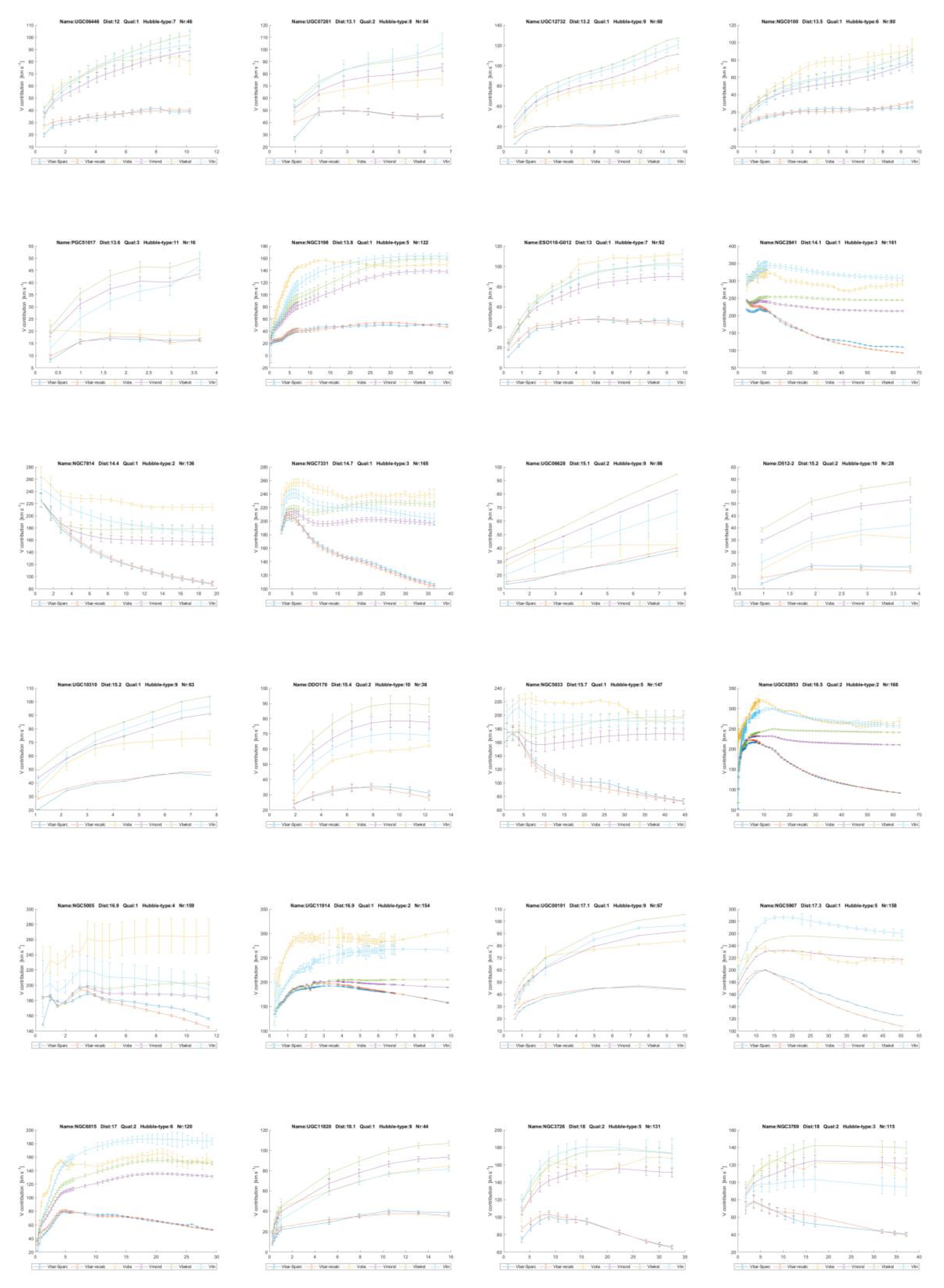
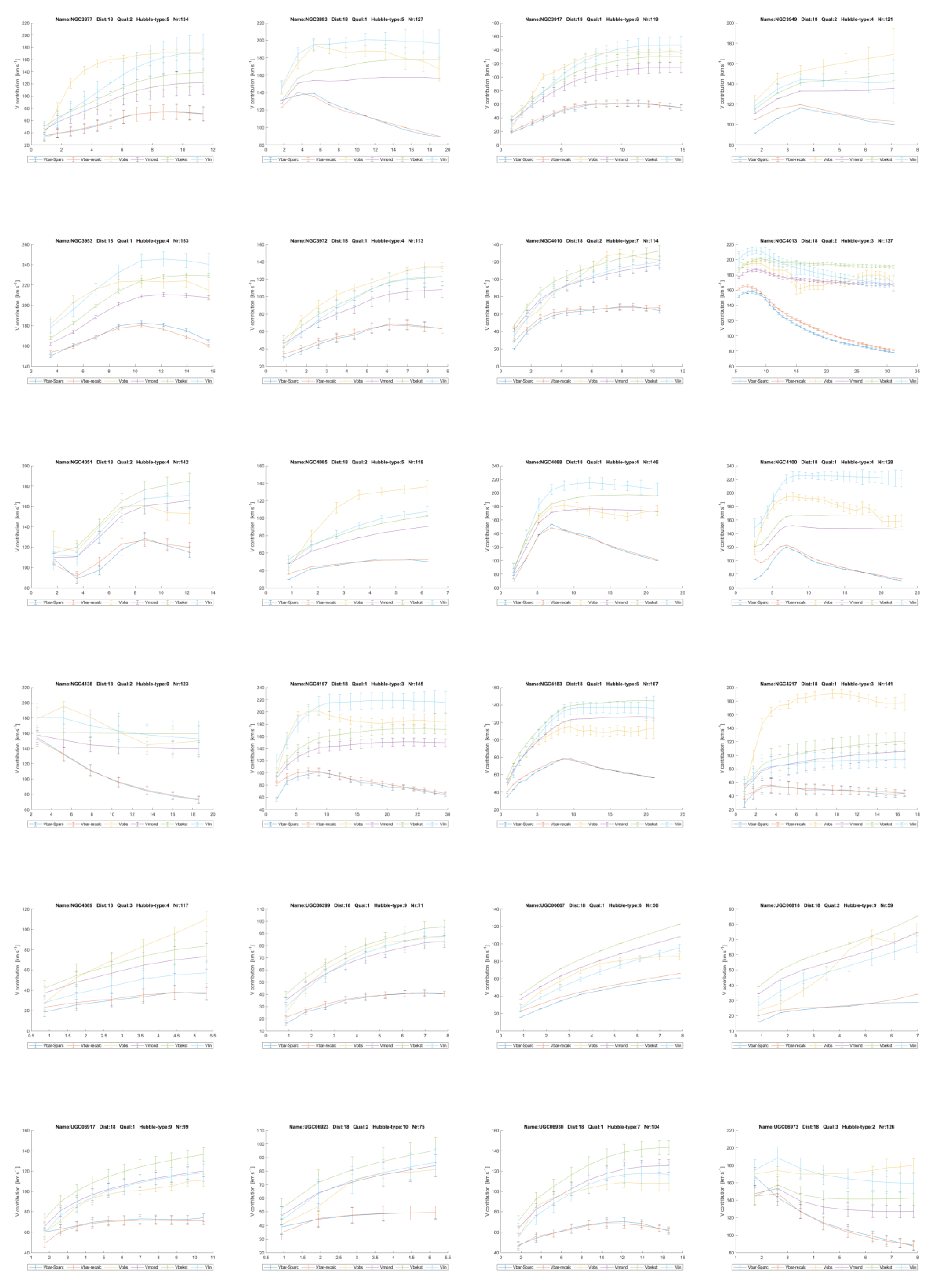
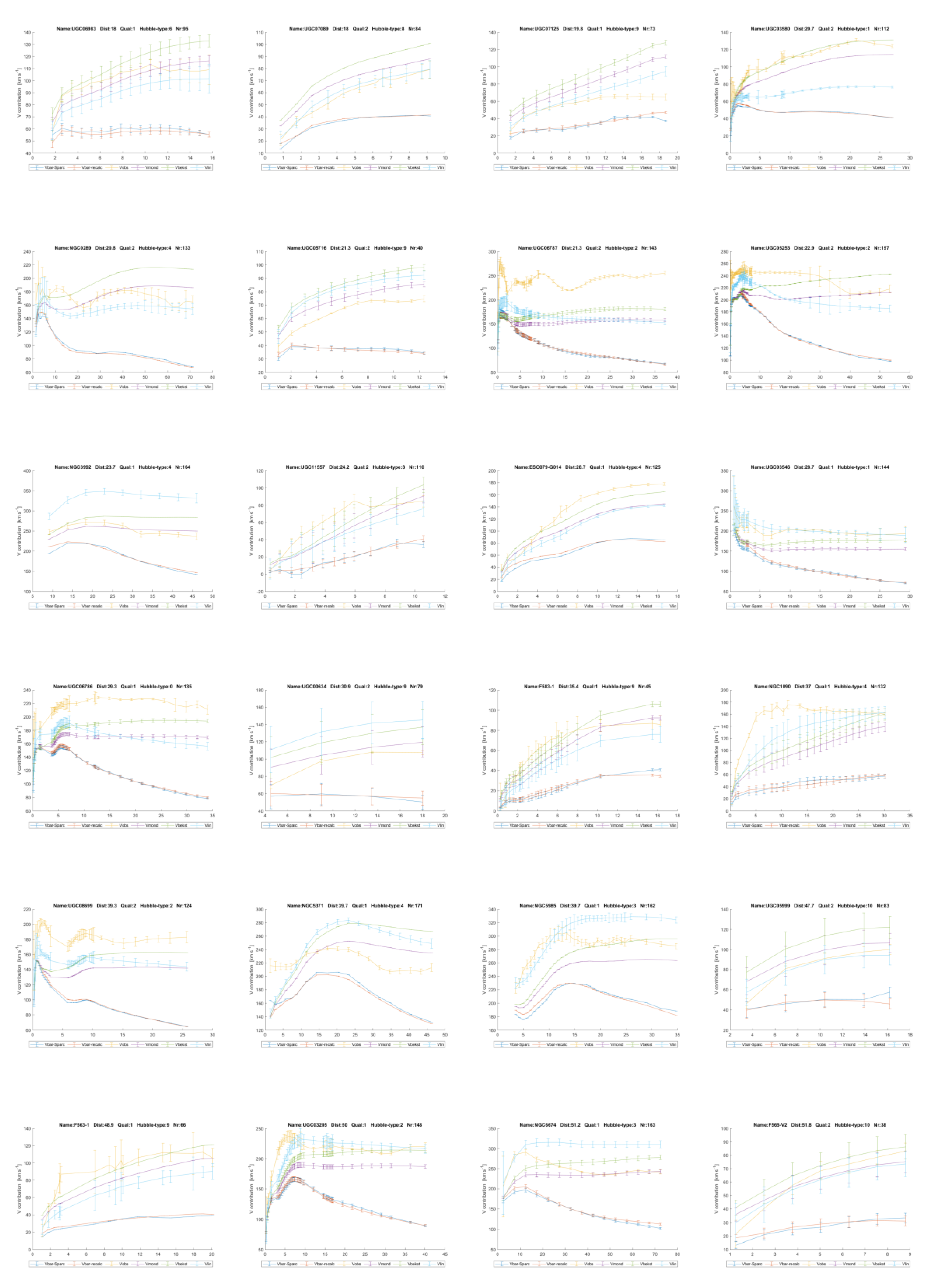
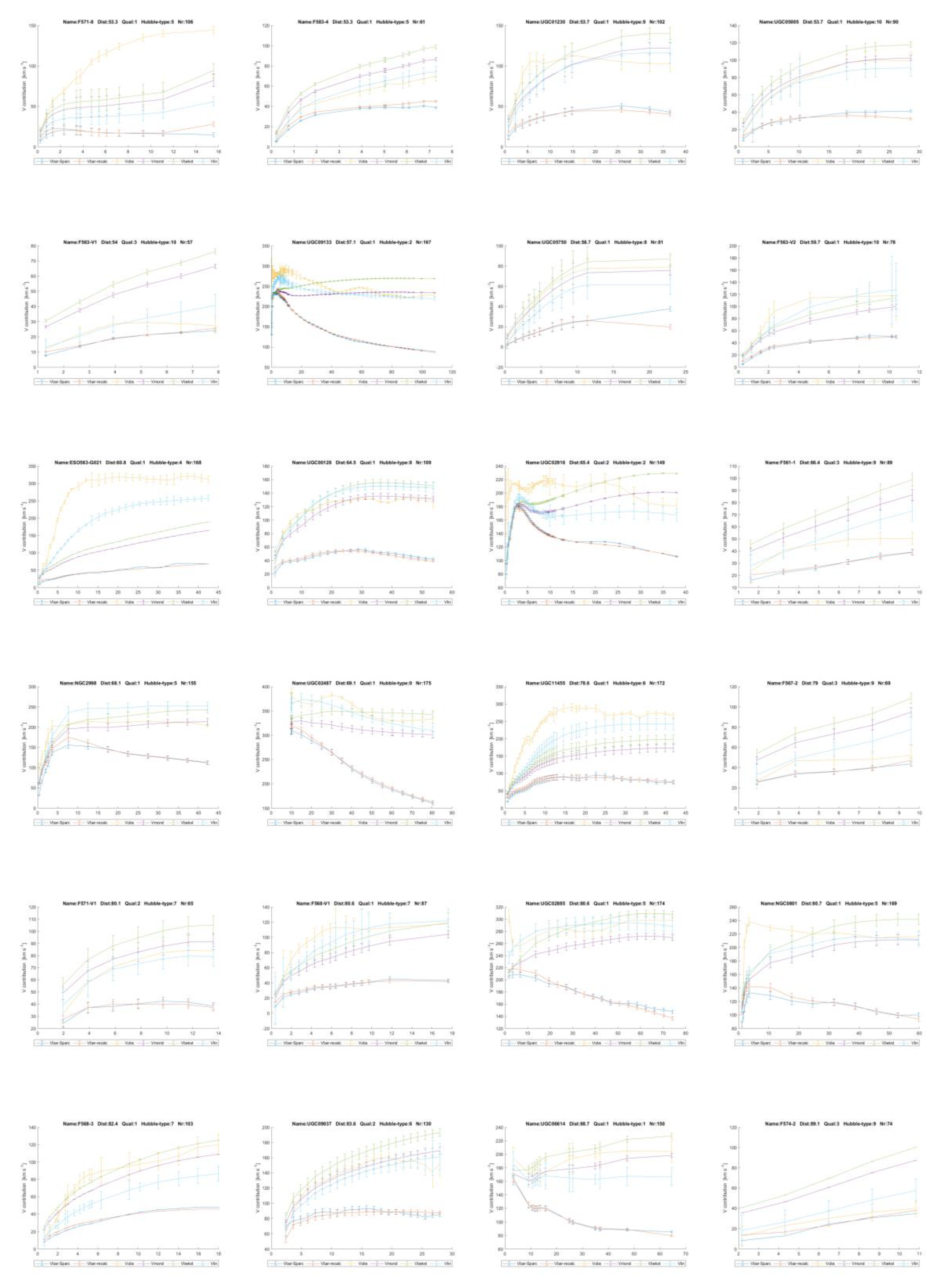
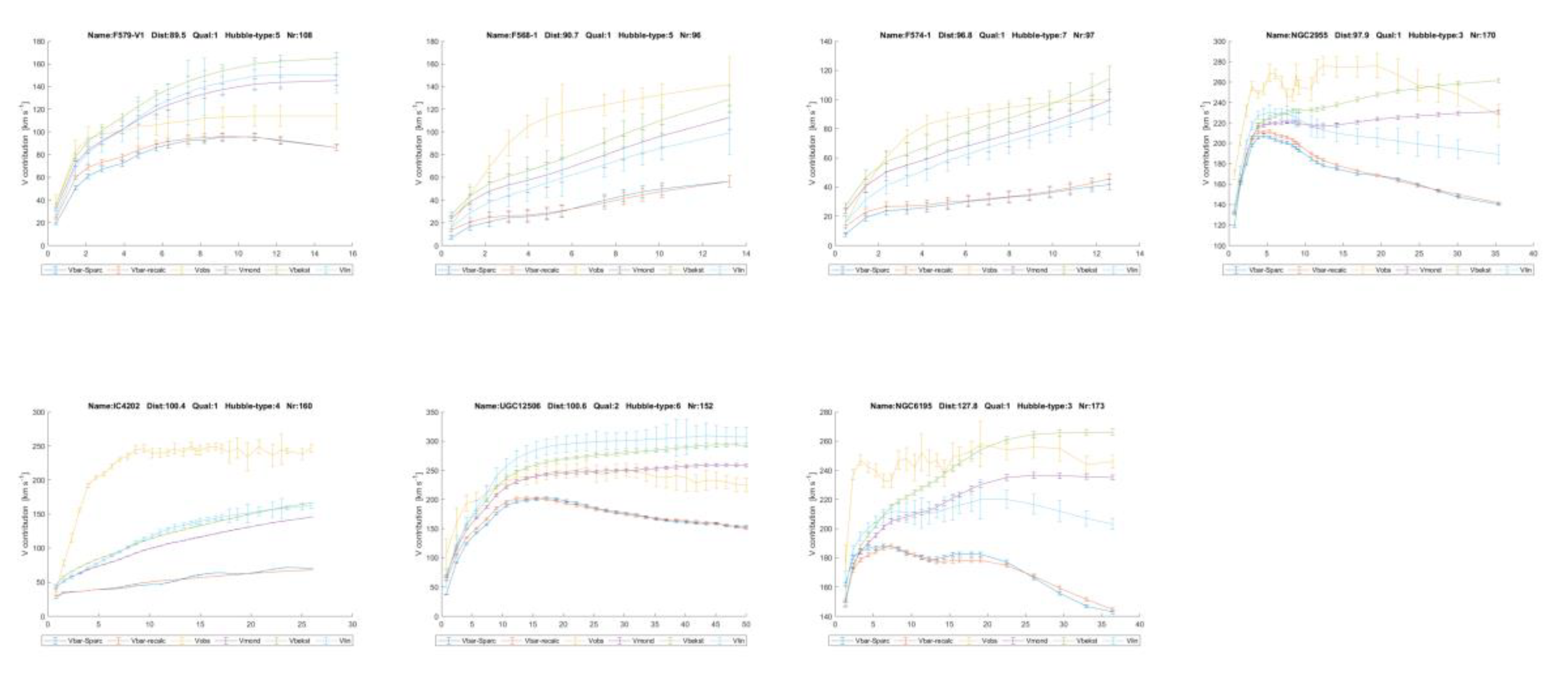
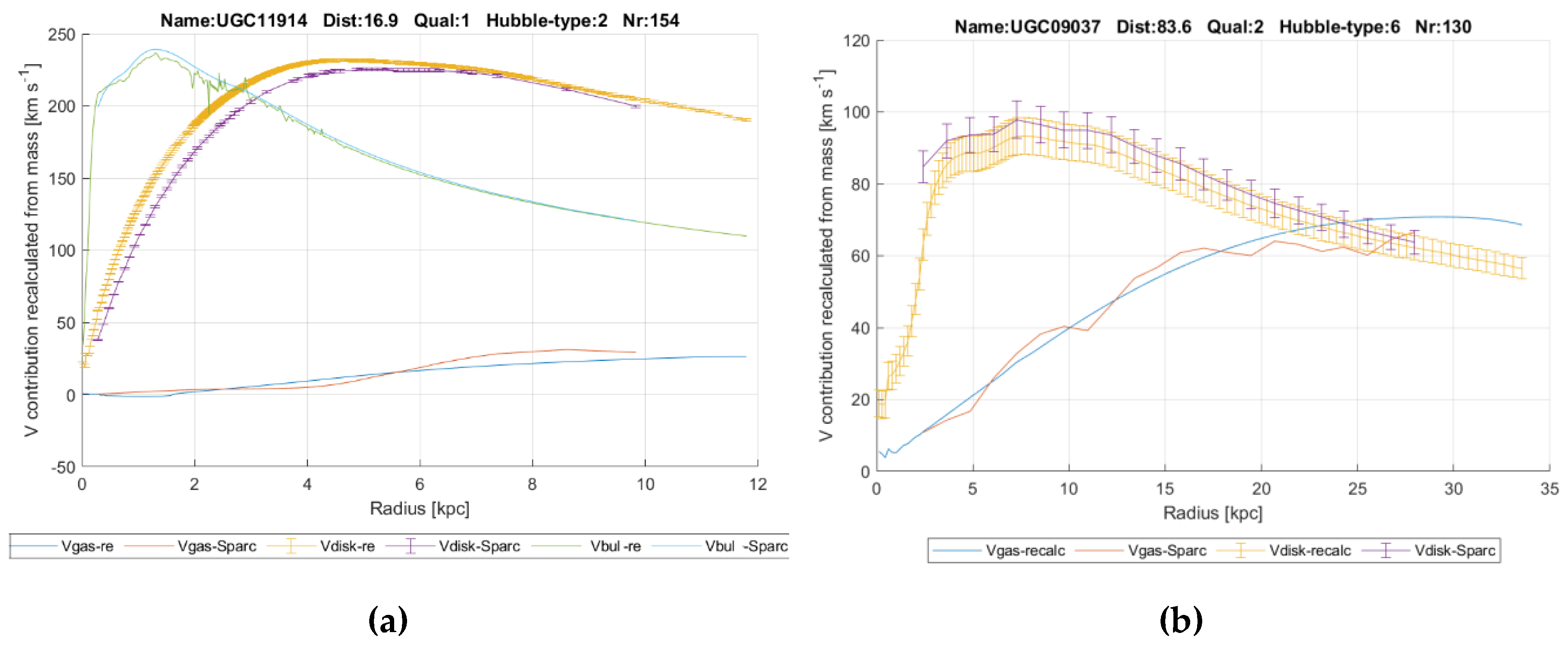
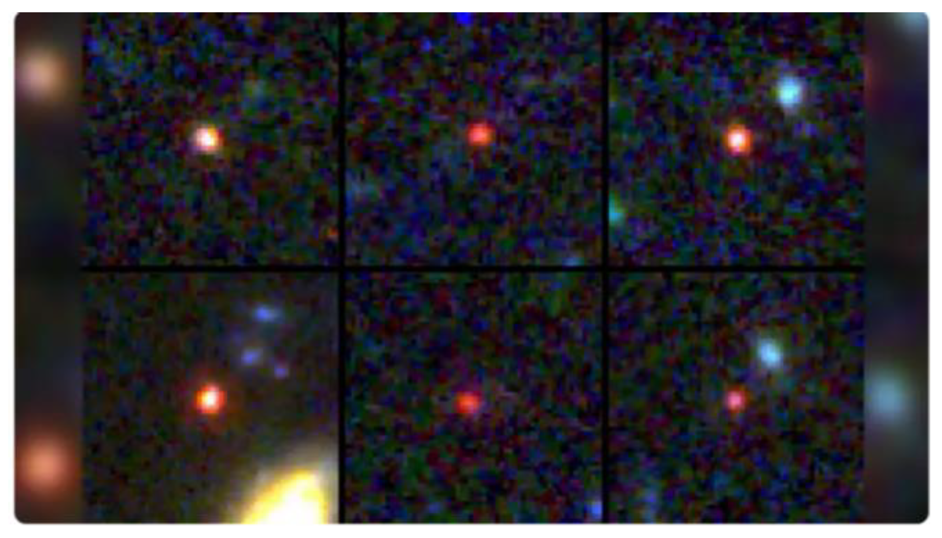
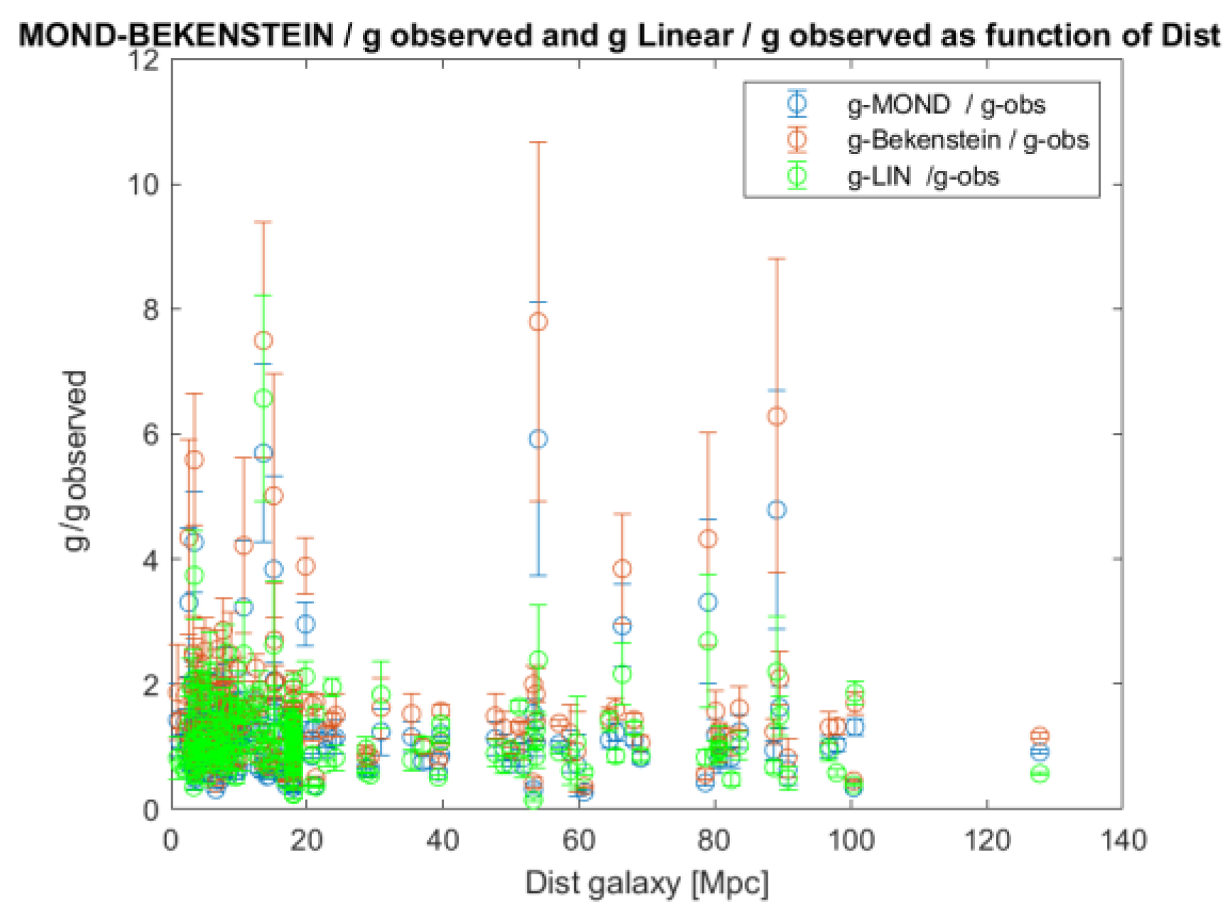
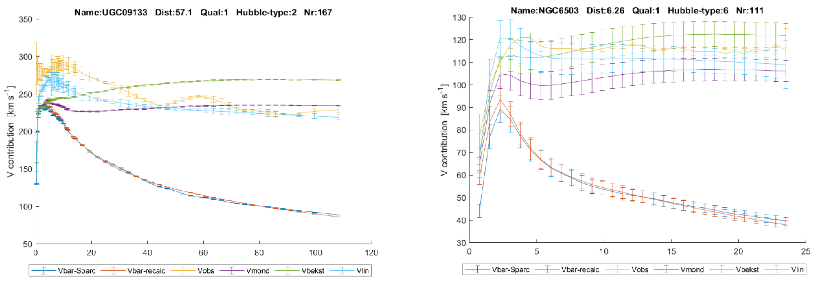
Hawking’s cosmology logically leads to an observed multiverse. This article argues it a superposition of at least three 3-dimensional universes in a 4-dimensional space, which each have two overlapping dimensions with the observed universe. For there is nothing outside it that could disturb the superposition, it could last forever. This explains why dark matter yields a linear decrease of gravity with distance to visible mass at large radii in galaxies. To prove this, all contributions of visible matter in the disks and bulges, calculated by the SPARC team, have been recalculated to verify the brightness and gas density are correctly interpreted. Lelli and Mistele showed the common way to project dark matter halos around galaxies cannot be valid. Since application of General Relativity would need these halos too, it must be modified with additional terms. Bekenstein’s TeVeS does this. Using TeVeS, a decay of the contribution of dark matter to gravity with the expansion of space is confirmed. This explains the rapid development of large galaxies in the early universe that is reported by Labbé. A new prediction method for rotation velocities that works at all radii in galaxies is offered. It is 25% more accurate than MOND and TeVeS.
Keywords:
1. Introduction
2. Hawking´s Cosmology and Superposition State of Universe
2.1. Big Bang Theory
2.2. Hawking´s Cosmology
2.3. Other Relevant Quantum Systems in a State of Superposition
3. Introduction to MOND and TeVeS Theories
4. A Hypothesis on the Nature of Dark Matter
4.1. Interpreting Linear MOND-Like Behaviour of Gravity
4.2. Exploring the Logical Consequences of Hawkings’s Cosmology
4.3. The Argument in Steps
- Hawking’s cosmology is a logical combination of two well proven theories, quantum mechanics and Big Bang theory, and thus, it is a good description of the earliest stages of our universe.
- Our universe results from a Big Bang that was in a quantum superposition state at its start, that can be interpreted as 10500 alternative histories in an 11-dimensional space, using the Feynman interpretation of quantum mechanics and M-theory.
- The realization of our universe from the 10500 alternative histories cannot have occurred without a sentient observer.
- Our universe has been realized.
- At least one sentient observer exists, which can have come into being in the universe following the conclusion of Wheeler’s delayed choice experiments.
- Since it is not economical to consider 10500 a fine-tuned number, aimed at creating exactly one universe with sentient being, there still remains a superposition state of more than one alternative histories of the universe. This makes it a multiverse, each universe with sentient beings. This multiverse still exists by means of a state of superposition, which must not necessarily be disturbed by de-coherence, since nothing exists outside the multiverse.
- The other universes in superposition can follow a history comparable with ours that leads to sentient beings, but do not necessarily share all our spatial dimensions in the 11-dimensional space, but do have nearly exactly the same constants of nature. From the delayed choice experiment it follows they all have the same causal status.
- The gravity of these superposed 11-dimensional universes acts together just like the binding force in a deuteron.
- Since there are more ways to yield partly overlapping universes in an 11-dimensional space than fully overlapping, the odds are that there exist multiple universes that share only one or two dimensions with our universe.
- Gravity acting in our universe resulting from the 2-dimensional projection of another one, leads to a linear decrease of the gravitational acceleration as a function of distance from a mass.
- The existence of multiple universes that share two dimensions with our universe in a state of superposition, forms a natural explanation for the linear MOND-like behaviour of gravity at large distances from the core of galaxies.
5. An Elaborated Proposal for Dark Matter
6. Testable Predictions
6.1. First Prediction
6.2. Second Prediction
6.3. Third Prediction
6.4. Fourth Prediction
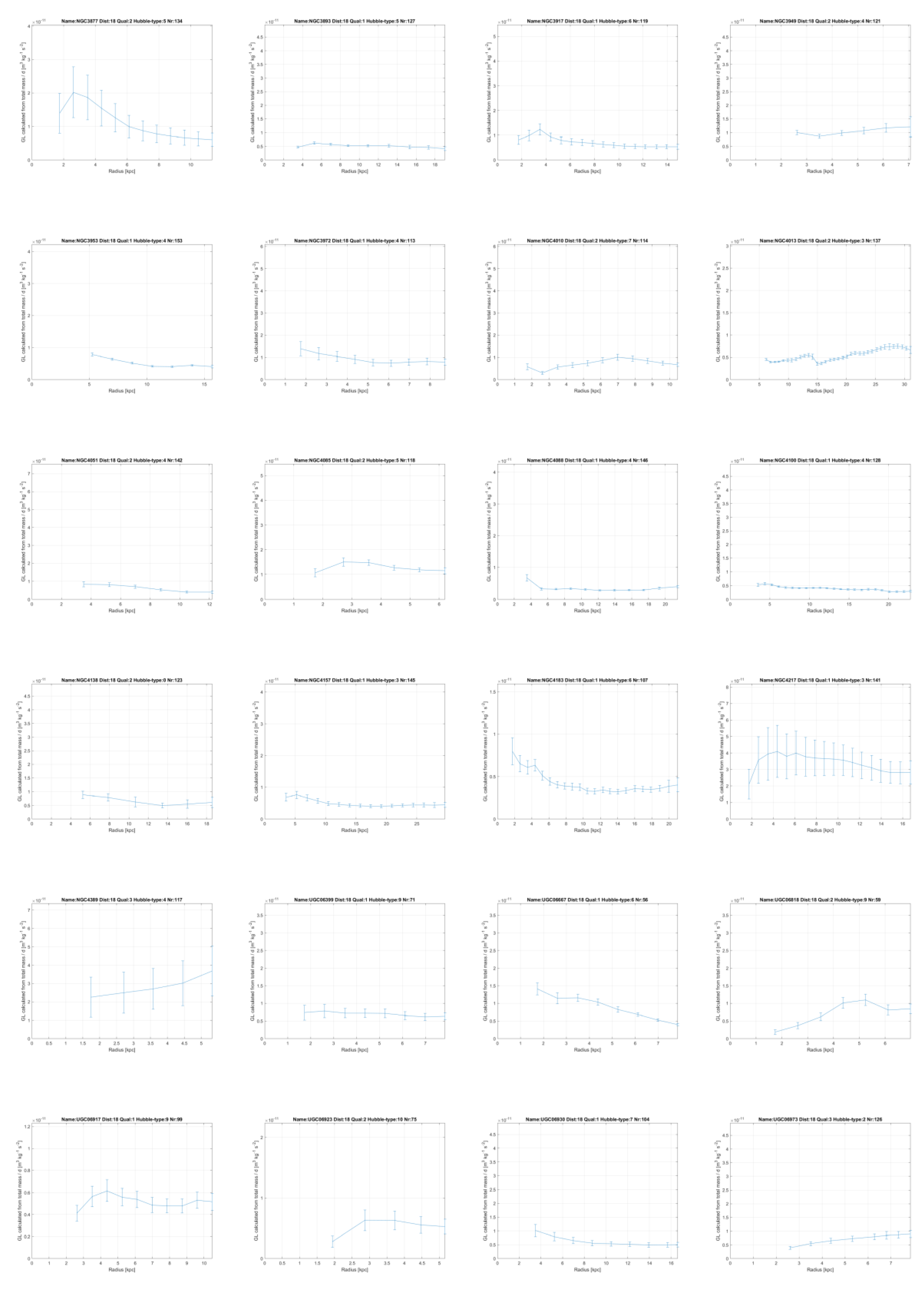
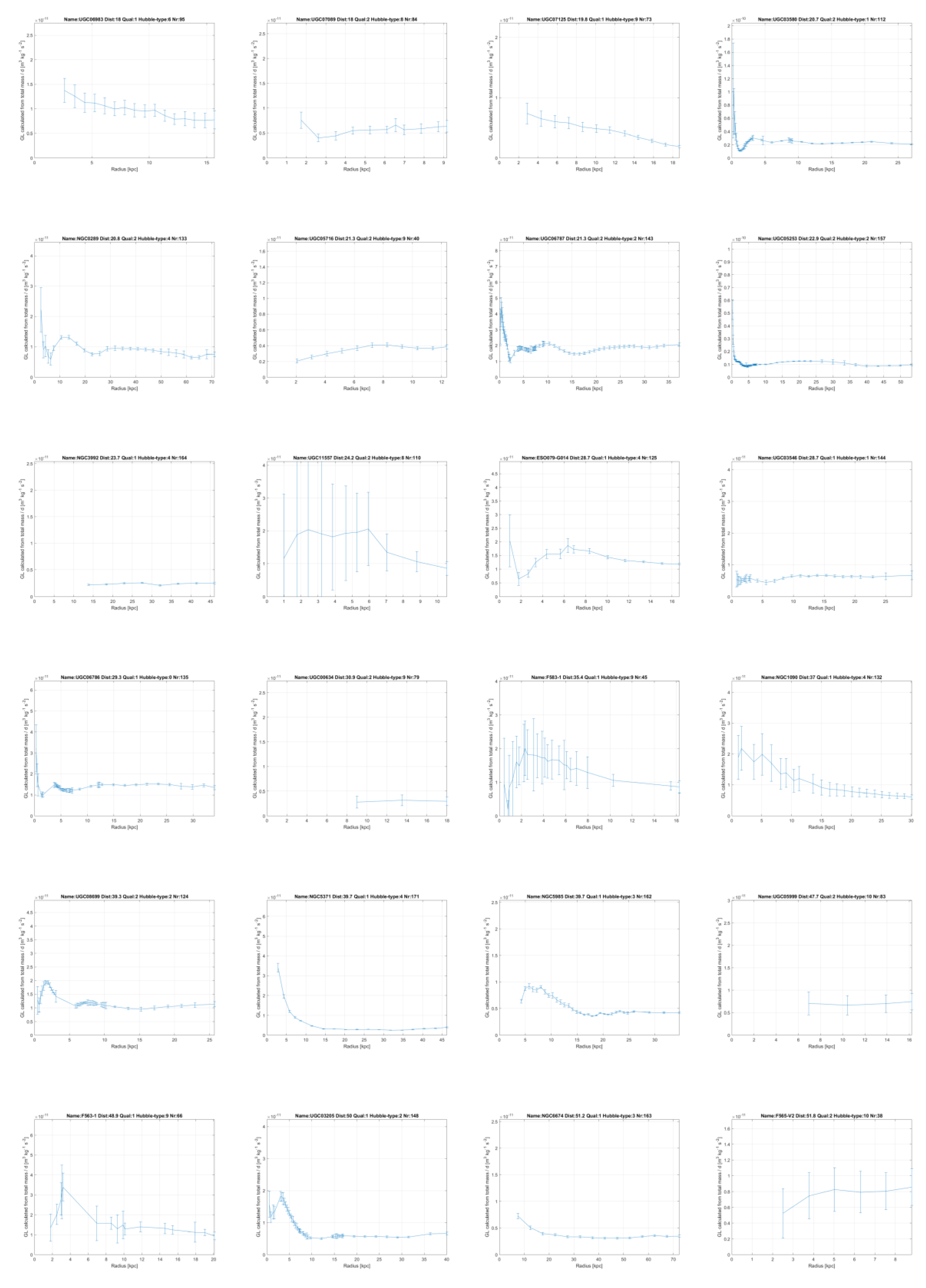
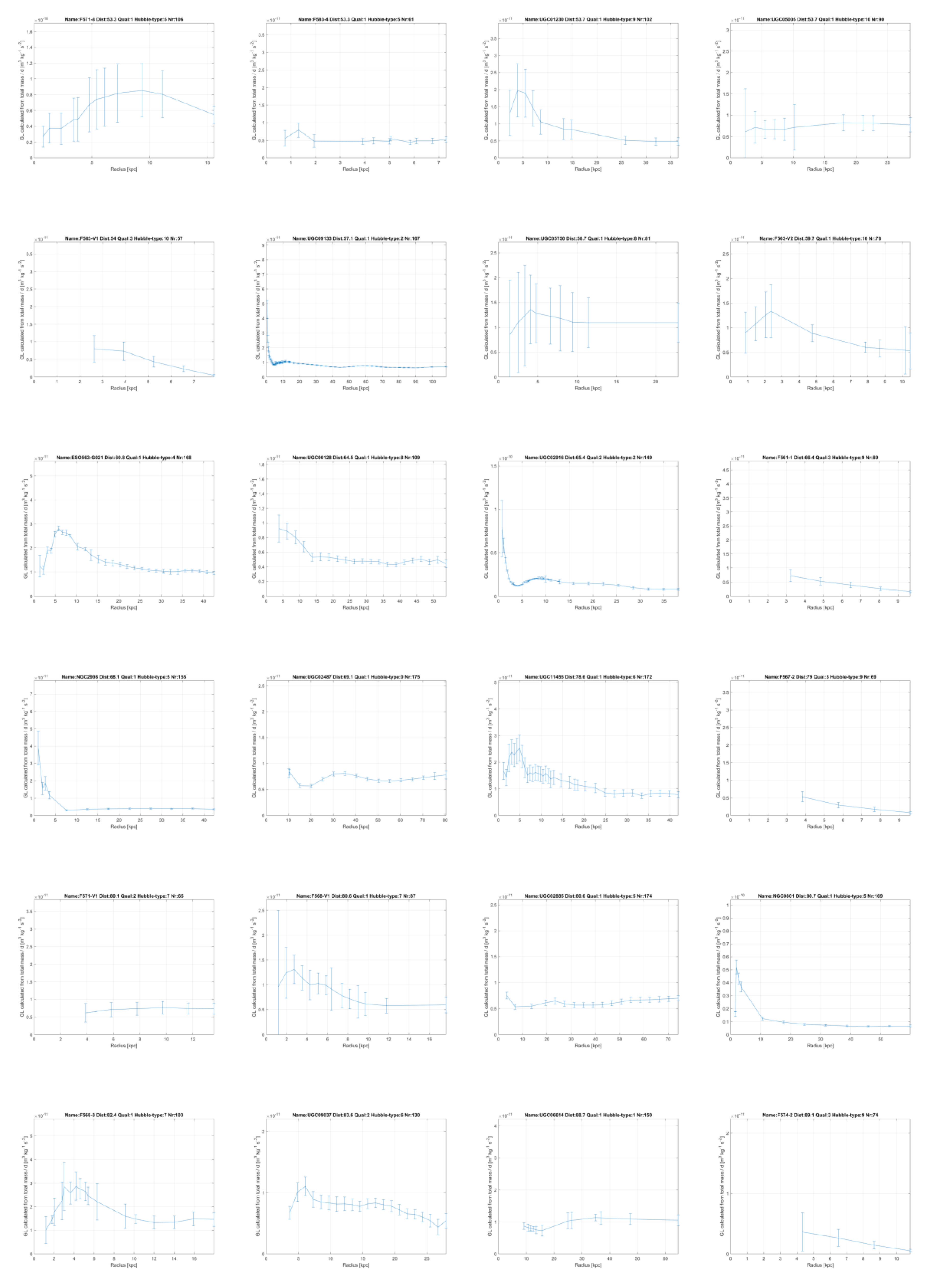
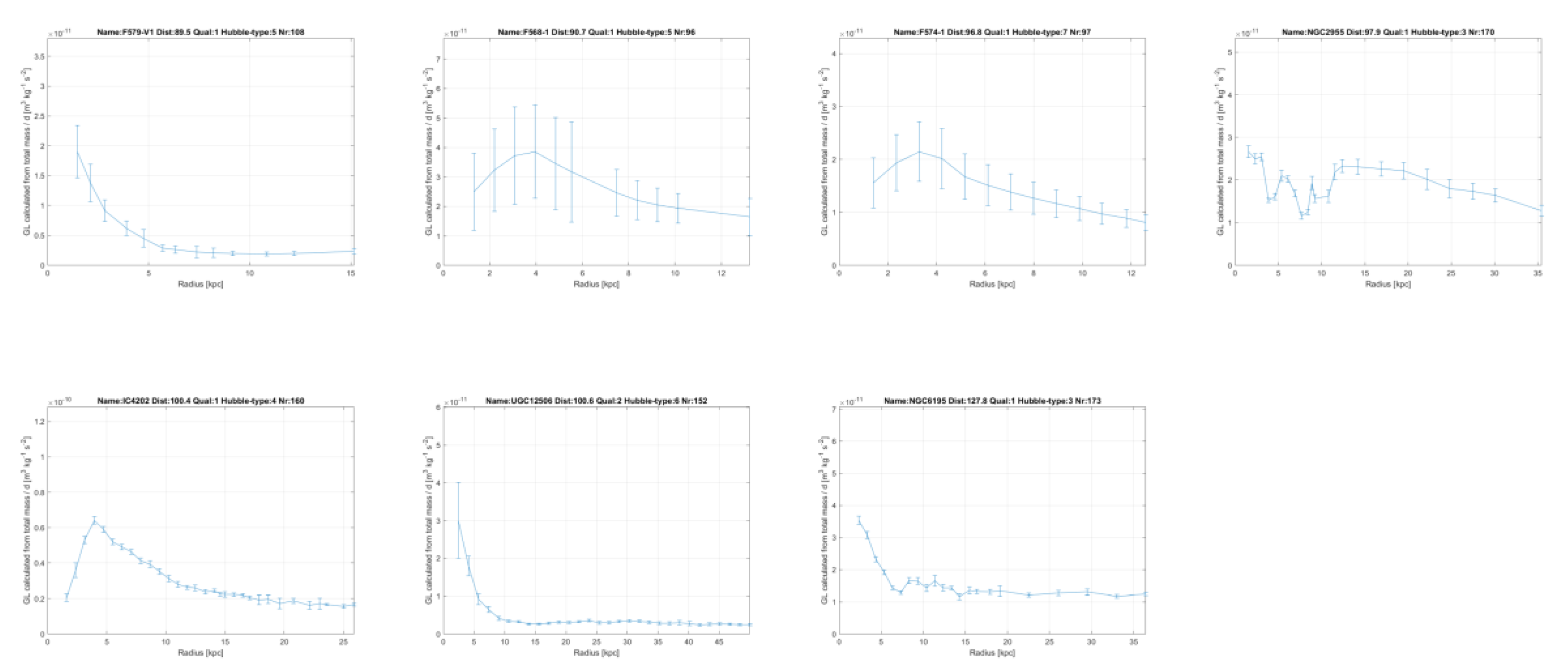
- Calculate the Newtonian gravitational acceleration at R, from the baryonic mass distribution with formula (13), for bulges with formula (14).
- From the same baryonic mass distribution, already available from step 1), calculate the sum of mass/distance at R, only taking the mass density in the rotation plane into account.
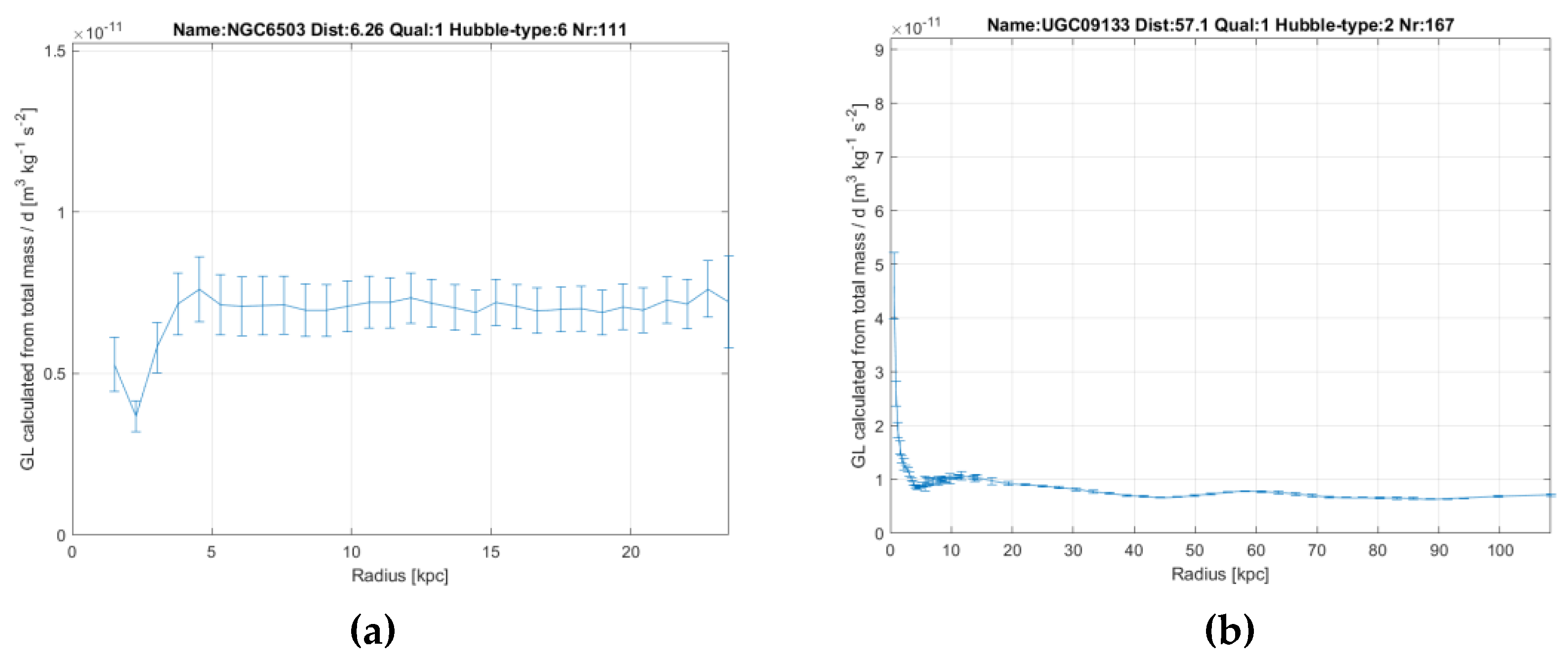
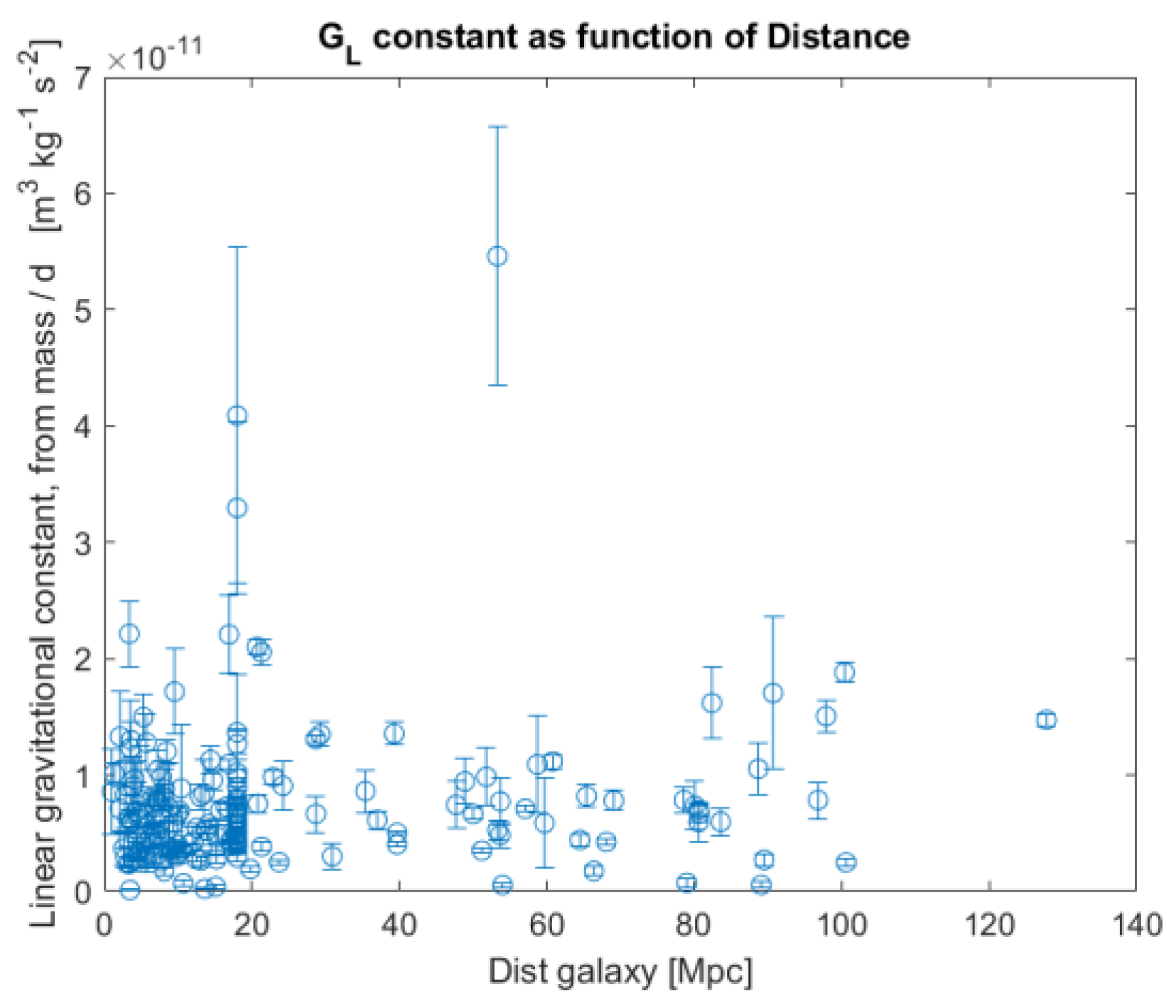
- Assuming a value GL ≈ 6.4 x 10⁻¹² [m3 kg-1 s-2], calculate the additional linear gravitational acceleration with formula (16).
- Correct the computed linear gravitational acceleration at time t with the ratio current radius of the universe / radius at time t.
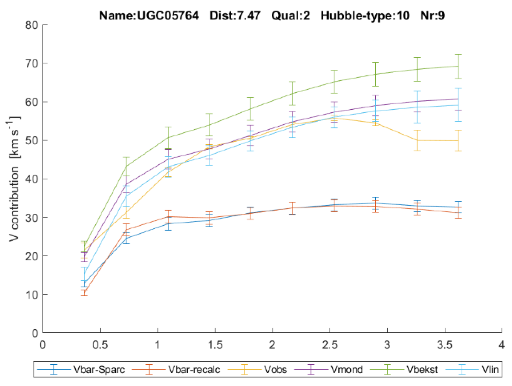
- Add the Newtonian gravitational acceleration to the linear gravitational acceleration and compute the rotation velocity with formula (12).
6.5. Fifth Prediction
6.6. Sixth Prediction
7. General Relativity and TeVeS Theory
7.1. Introducing and Applying TeVeS
7.2. Evolution in Time
7.3. Application
8. Conclusions and Suggestions for Further Work
Annexes

References
- Milgrom, M. A modification of the Newtonian dynamics as a possible alternative to the hidden mass hypothesis. Astrophys. J. 1983, 270, 365–370. [Google Scholar] [CrossRef]
- Milgrom, M. A modification of the Newtonian dynamics—Implications for galaxies. Astrophys. J. 1981, 270, 371. [Google Scholar] [CrossRef]
- Milgrom, M. A modification of the newtonian dynamics—Implications for galaxy systems. Astrophys. J. 1983, 270, 384. [Google Scholar] [CrossRef]
- Bekenstein, J.D. Relativistic gravitation theory for the modified Newtonian dynamics paradigm. Phys. Rev. D 2004, 70, 083509. [Google Scholar] [CrossRef]
- Verlinde, E.P. Emergent Gravity and the Dark Universe. SciPost Phys. 2017, 2, 016. [Google Scholar] [CrossRef]
- Verlinde, E. On the origin of gravity and the laws of Newton. J. High Energy Phys. 2011, 2011, 1–27. [Google Scholar] [CrossRef]
- Hartle, J.B.; Hawking, S.W. Wave function of the Universe. Phys. Rev. D 1983, 28, 2960–2975. [Google Scholar] [CrossRef]
- Hawking, S.W.; Mlodinow, L. The Grand Design; Bantam Press and Transworld Publishers: London, UK, 2010. [Google Scholar]
- Mistele, T.; McGaugh, S.; Lelli, F.; Schombert, J.; Li, P. 2024, Indefinitely Flat Circular Velocities and the Baryonic Tully-Fisher Relation from Weak Lensing. arxiv 2024, arXiv:2406.09685v1. [Google Scholar]
- Hossenfelder S. 2019, (German translation) Das Hässliche Universum, Warum unsere Suche nach Schönheit die Physik in die Sackgasse führt (4th edition; S. FISCHER Verlag, Frankfurt am Main, Germany) (original title: Lost in Math, How Beauty leads Physics astray, Basic Books, New York, USA).
- Lelli, F.; McGaugh, S.S.; Schombert, J.M. Sparc: mass models for 175 disk galaxies with spitzer photometry and accurate rotation curves. Astron. J. 2016, 152, 157. [Google Scholar] [CrossRef]
- Starkman, N. et al. 2018, A New Algorithm to Quantify Maximum Discs in Galaxies, MNRAS 000, 1–10 (2018).
- Heuvel E. P. J. Van den 2012, Oerknal, Oorsprong van de eenheid van het heelal (Big Bang, Origin of the unity of the universe)(Veen Magazines B.V., Diemen, The Netherlands).
- Everett, H. Relative State Formulation of Quantum Mechanics. Rev. Mod. Phys. 1957, 29. [Google Scholar] [CrossRef]
- DeWitt, B.S. Quantum Theory of Gravity. I. The Canonical Theory. Phys. Rev. 1967, 160, 1113–1148. [Google Scholar] [CrossRef]
- Griffiths, D.J.; Schroeter, D.F. Introduction to Quantum Mechanics, 3rd ed.Cambridge University Press: Cambridge, UK, 2018. [Google Scholar]
- Bethe, H.A. A Meson Theory of Nuclear Forces, Part II, Theory of the Deuteron. Phys. Rev. 1940, 57, 390. [Google Scholar] [CrossRef]
- Khalili J. Al-, McFadden J. 2015, (Dutch translation) Hoe leven ontstaat, op het snijvlak van biologie en kwantumleer (Atlas Contact, Amsterdam, The Netherlands) (original title: Life on the Edge, Transworld, London, UK, 2015).
- Kroupa, P.; Jerabkova, T.; Thies, I.; Pflamm-Altenburg, J.; Famaey, B.; Boffin, H.M.J.; Dabringhausen, J.; Beccari, G.; Prusti, T.; Boily, C.; et al. Asymmetrical tidal tails of open star clusters: stars crossing their cluster's path challenge Newtonian gravitation. Mon. Not. R. Astron. Soc. 2022, 517, 3613–3639. [Google Scholar] [CrossRef]
- Schilling G. 2021, (Dutch translation) De Olifant in het Universum, Donkere materie, mysterieuze deeltjes en de samenstelling van ons heelal (Fontaine Uitgevers, Amsterdam, The Netherlands) (original title: The Elephant in the Universe, Harvard University Press, 2021).
- Platschorre, A.D. On Covariant Emergent Gravity. Bachelor’s Thesis, Delft University, Delft, The Netherlands, 2019. [Google Scholar]
- Bekenstein, J.D. Phase coupling gravitation: Symmetries and gauge fields. Pys. Lett. B 1988, 202, 497. [Google Scholar] [CrossRef]
- Rees, M. Just Six Numbers; Basic Books: New York, NY, USA, 2000. [Google Scholar]
- Lemaître, A.G. Contributions to a British Association Discussion on the Evolution of the Universe. Nature 1931, 128, 704–706. [Google Scholar] [CrossRef]
- Darling D. 2006, (Dutch translation) Zwaartekracht, van Aristoteles tot Einstein en verder (Uitgeverij Veen Magazines, Diemen, The Netherlands), (original title: Gravity’s Arc, John Wiley & Sons, Hoboken, USA, 2006).
- Han, J.J.; Conroy, C.; Hernquist, L. A tilted dark halo origin of the Galactic disk warp and flare. Nat Astron 2023, 7, 1481–1485. [Google Scholar] [CrossRef]
- Martinsson, T.P.; Verheijen, M.A.; Bershady, M.A.; Westfall, K.B.; Andersen, D.R.; Swaters, R.A. The DiskMass Survey. X. Radio synthesis imaging of spiral galaxies. Astron. Astrophys. 2016, 585, A99. [Google Scholar] [CrossRef]
- Ku, H.H. Notes on the use of propagation of error formulas. J. Res. Natl. Bur. Stand. 1966, 70C. [Google Scholar] [CrossRef]
- Kruit P.C. van der, Freeman K.C. 2010, Galaxy disks, Kapteyn Astronomical Institute, University of Groningen, The Netherlands.
- Sparke, L.S. , Gallagher S. Galaxies in the Universe, An introduction, 2nd ed.; Cambridge University Press: Cambridge, UK, 2007. [Google Scholar]
- de Grijs, R. The global structure of galactic discs. Mon. Not. R. Astron. Soc. 1998, 299, 595–610. [Google Scholar] [CrossRef]
- Begelman, M. , Rees, M. Gravity’s Fatal Attraction, Black Holes in the Universe, 3rd ed.; Cambridge University Press: Cambridge, UK, 2021. [Google Scholar]
- Riess, A.G.; Yuan, W.; Macri, L.M.; Scolnic, D.; Brout, D.; Casertano, S.; Jones, D.O.; Murakami, Y.; Breuval, L.; Brink, T.G. . A Comprehensive Measurement of the Local Value of the Hubble Constant with 1 km s 1 Mpc 1 Uncertainty from the Hubble Space Telescope and the SH0ES Team. Astrophys. J. Lett. 2022, 934, L7. [Google Scholar] [CrossRef]
- Labbé, I.; van Dokkum, P.; Nelson, E.; Bezanson, R.; Suess, K.A.; Leja, J.; Brammer, G.; Whitaker, K.; Mathews, E.; Stefanon, M.; et al. A population of red candidate massive galaxies ~600 Myr after the Big Bang. Nature 2023, 616, 266–269. [Google Scholar] [CrossRef] [PubMed]
- Zeilinger, A. Experiment and the foundations of quantum physics. Rev. Mod. Phys. 1999, 71, S288–S297. [Google Scholar] [CrossRef]
- Schutz, B.F. A First Course in Genaral Relativity; Cambridge University Press: Cambridge, UK, 2003. [Google Scholar]
- Zhang, P.; Liguori, M.; Bean, R.; Dodelson, S. Probing Gravity at Cosmological Scales by Measurements which Test the Relationship between Gravitational Lensing and Matter Overdensity. Phys. Rev. Lett. 2007, 99, 141302. [Google Scholar] [CrossRef]
- Seifert, M.D. Stability of spherically symmetric solutions in modified theories of gravity. Phys. Rev. D 2007, 76, 064002. [Google Scholar] [CrossRef]
- Matlab 2021, MATLAB® is a registered trademark and MATLAB Grader is a trademark of The MathWorks, Inc, Natick, USA.

| Yml | MOND vs. glinear+gbar | TeVeS vs. glinear+gbar |
|---|---|---|
| Fitted | 24 % | 26 % |
| 0.5 | 23 % | 27 % |
Disclaimer/Publisher’s Note: The statements, opinions and data contained in all publications are solely those of the individual author(s) and contributor(s) and not of MDPI and/or the editor(s). MDPI and/or the editor(s) disclaim responsibility for any injury to people or property resulting from any ideas, methods, instructions or products referred to in the content. |
© 2024 by the authors. Licensee MDPI, Basel, Switzerland. This article is an open access article distributed under the terms and conditions of the Creative Commons Attribution (CC BY) license (http://creativecommons.org/licenses/by/4.0/).


