

Submitted:
31 October 2025
Posted:
04 November 2025
You are already at the latest version
Abstract
Hawking’s cosmology logically leads to an observed multiverse. This article proposes a novel hypothesis for the physical nature and existence of dark matter, derived from his cosmology This article argues it is a superposition of at least three 3-dimensional universes in a 4-dimensional space, of which two dimensions overlap with our universe. Nothing that could disturb the superposition exists outside it. This, with the dimensions of strings in String theory, explains why dark matter causes a linear decrease in gravity with distance to visible mass at large radii in galaxies. To support this, the visible matter distribution in the disks and bulges, calculated by the SPARC team, and the observed rotation velocities are used. Lelli and Mistele showed that the common way to project dark matter halos around galaxies cannot be valid. In this article it is shown a valid alternative is to model dark matter as three added wire-like masses in the centre of galaxies in General Relativity.Linear mass density is a key parameter and explains the weak effect in the centre of galaxies and the strong effect at larger distances as well as the rapid development of large galaxies in the early universe as reported by Labbé. A new prediction method for rotation velocities, that works at all radii in galaxies, is 19 % more accurate than MOND. In galaxy clusters the improvement of the predicted velocity dispersions compared with the Newtonian approach and with MOND is 44 to 57 % over a huge range of cluster masses.
Keywords:
dark matter
; galaxies
; clusters
; SPARC
; multiverse
; superposition
; linear gravity
; naturalness
1. Introduction
The hypothesis of dark matter is a way to explain why among other galaxies seem not to obey Newton’s law of gravity. As well, dark matter is needed to explain the statistical distribution of ‘cold’ and ‘hot’ spots in the background radiation, that would still need the existence of (much) dark matter vs. baryonic matter to be understandable in terms of Big Bang nucleosynthesis, as well as matters like gravitational lensing. In this article it will be argued dark matter is a physical entity arising from the multiverse hypothesis.
Nevertheless, there exist several alternative approaches to account for the additional gravity it yields, like Modified Newtonian Dynamics (MOND) [1,2], Bekenstein’s TensorVectorScalar gravity (TeVeS) [3] or Covariant Emergent Gravity (CEG) [4]. But, they assume dark matter does not really exist, and so leave the other matters mentioned up here, and the gravity in galaxy clusters, see Banik [2], unresolved. Besides that, they do not give a natural explanation for the concepts and additional fields they introduce.
Therefore, in the article in hand the existence of dark matter is the starting point.
So as to describe its effect on gravity, it applies the cylindrically symmetric solution of the Einstein field equations from Levi-Civita [5] as described by Santos [6] in linearized or numerical General Relativity (GR). and properly described by a linear mass density. Dark matter appears as wire-masses because the fourth dimension at the level of strings is interwoven with our universe and is rolled up at the GUT-scale, which however is much larger than the Planck-length, the assumed size of the fourth dimension at the start of the Big Bang (Hawking 2010). This is because the effective distances gravity has to act over in another universe, are thus being much longer. So, this hypothesis may bring the smallest and large scales together.
It solves the problem that Lelli and Mistele [9] showed, that the common way to project dark matter halos around galaxies cannot be valid, since the alternative naturally assumes dark matter is distributed like the visible matter in a galaxy, but in a wire-mass shape, consistent with [5] and [6]. The hypothesis gives a natural explanation of dark matter, why it is undetectable and why its gravity shows flat rotation curves at large distances from the galaxy centre and Newtonian behaviour, and even allows elliptical orbits of stars, near the centre. The term naturalness is extensively discussed by Hossenfelder [10] (p. 57). In short it means that a theory is without fine-tuned constants.
In this paper the Spitzer Space Telescope satellite data of 175 galaxies, SPARC, as processed and reported by Lelli et al. [11] and Starkman et al [12] are used to assess several predictions that follow from this theory. The mass-to-light ratio has been used as the only fitting parameter to fit the baryonic rotation velocity, and hence the baryonic gravitational acceleration, in each galaxy to the observed values near the centre of the galaxies. After that, the hypothesis in hand is used to predict the additional gravitational acceleration at all radii without any further fitting and to compare the predictions with the observed values.
After a brief introduction of Big Bang theory in chapter 2.1 and Hawking’s cosmology in chapter 2.2 and some other indispensable literature about quantum systems in chapter 2.3, MOND and TeVeS will be discussed in chapter 2.4. This forms the fundament for the proposal presented in chapter 3.
In chapter 3 the proposal will stepwise be derived in a logical manner from Hawking’s cosmology and String theory.
In chapter 4 this will all be worked out. Firstly, an interpretation of the MOND like behaviour of dark matter as a sum of two fields will be proposed. Secondly, the natural basis for this will be explored in chapter 4.2 and in chapter 4.3. In the rest of chapter 4, the hypothesis for dark matter will be elaborated and its consequences and behaviour will be explored.
In chapter 5, seven testable predictions are proposed and proved, one using the work of Levi-Civita, and in chapter 5.3 an improved alternative to MOND for the prediction of rotation velocities is presented.
In chapter 5.4 it will be shown it gives a much improved prediction for dispersion velocities in a wide range of NGC and Abell clusters and that this can explain the rapid development of large galaxies in the early universe. The rest of chapter 5 gives three other predictions.
In chapter 6 the conclusions and suggestions for further work are presented.
2. Hawking´s Cosmology and Superposition State of Universe, MOND and TeVeS
In this chapter the fundament for the proposal of chapter 3 will be laid, by giving an overview of existing theories that contain vital building elements.
2.1. Big Bang Theory
The line of thought of the universe as a quantum system is an elaboration of Hartle & Hawking [7]. The universe, according to the Big Bang theory, comes from an infinitesimal small point in which only elementary particles existed in the form of a plasma, with an extremely high temperature [13] (pp. 127-136) and as a result was in a quantum state, see chapter 4.
The originally extremely high temperature is still visible and measurable in the so-called background radiation. Its properties are direct evidence that the universe originated from a hot Big Bang stage. The Big Bang theory is also a logical extrapolation of the expansion of the universe that we observe, among other things due to the redshift of the spectrum of the radiation of stars, but also of the history/evolution of stars and galaxies as visible through our telescopes.
In addition, the non-uniform distribution of stellar objects as quasars over the different redshifts proves the universe is not static.
Moreover, Big Bang theory can quantitatively explain many phenomena, such as the distribution over the various elements of the mass in the universe, the cosmic composition, based on nuclear physics.
The fact that it is dark at night also proves that the universe cannot be infinitely large and infinitely old, because then the entire sky would be filled with light from stars. So, our universe indeed has a beginning. Moreover, the Big Bang theory forms a well-cohesive whole with astronomy and the rest of physics.
2.2. Hawking´s Cosmology and String theory
Somewhere at the beginning, our universe has been in a quantum state, because that's where one ends upon extrapolating the expansion of the universe back to the very smallest starting point, [7,8] have derived solutions to the wave function of the universe as proposed by Everett [14] and further elaborated by DeWitt [15]. As derived and explained by Hartle & Hawking [7] these solutions must satisfy the Wheeler-DeWitt equation.
Hartle & Hawking [7] show the Wheeler-DeWitt equation has the following form:
(1)
Where is the wave function of the universe and where H ^ ( x ) Ĥ(x) is called the Hamiltonian constraint, [7]. The Hamiltonian, in this case derived from General Relativity [7], describes the total energy of a system and is the Hamiltonian operator [16] (p. 27). The so-called constraint described by (1) follows from the total energy of the universe being zero, gravitational energy cancelling out the mass energy. Hawking’s & Hartle’s solutions of this equation describe a universe that has no beginning, the Hartle-Hawking state, [7]. Hawking [8] explains this in simpler terms as well: time must have been indeterminate there on the smallest scale in that quantum state, because of the extreme gravitational warpage of space-time at that moment, [8] (p. 172). The time t=0 therefore is not precisely defined and at these scales time reduces to a fourth spatial dimension.
So, the universe has no exact measurable beginning. Hawking calls this the ‘no-boundary-condition’, [8] (pp. 172-173). It makes it impossible to trace the development of our universe from the beginning to this time in a deterministic ‘bottom-top’ way and, hence, there is a need for a statistical ‘top-down cosmology’, considering all possible alternative histories of the universe.
He states that as a consequence of this, at the very beginning time acted as a fourth spatial dimension, ”In the early universe-when the universe was small enough to be governed by both general relativity and quantum theory, there were effectively four dimensions of space and none of time”, [8] (p. 172) This is the starting point of the proposal of this paper. String theory, however, suggests as much as eleven dimensions, but using the minimum of four is more economical and easier to understand.
The quantum aspects of the Big Bang become clearer when considering so-called ‘double-slit’ experiments, with a light beam split in two that are directed at a wall with two narrow slits. Especially the variant where only one photon is fired at a time. The same interference patterns then arise as with continuous beams of photons, so the probability waves of single photons interfere with themselves, as it were. One photon behaves as if it passed through both slits. That can only happen if the photon itself follows all possible alternative paths simultaneously, as it were like a split probability wave. So, the behaviour of the single photon can be seen as a superposition of all possible alternative paths it follows, so alternative histories, [8] (p.104). The superposition causes wave interference and that determines the paths the photon follows in the experiment.
Hawking’s and other’s point about the probabilities is that a quantum experiment will only have a certain outcome when it is performed. The Big Bang can be regarded as such an experiment [8] p. 179), where the universe in the quantum state may have had a statistical probability distribution of many ‘alternative histories’, following the interpretation of Feynman. Maybe 10500 ones as String theory and the more general M theory suggest, [8] (pp. 152 and 181). At page 77 Hawking states that “the universe does not have a single existence or history, but rather every possible version of the universe exists simultaneously in what is called a quantum superposition”.
This does not a-priori imply we still are in a real a state of superposition between all, or part of these alternative histories now, but this paper will argue that this is indeed the case with our universe for a specific part of these histories.
The parameters and hence the quantum state of our universe are known now. Our universe has known single values for the fundamental parameters and constants. Of all the ‘alternative histories’, ours is the one that has come true. The experiment has been performed; we know the outcome. This is only possible when there is an observer to the experiment, [8] (pp. 107 and 179). This where the idea of an ‘observed universe’ of Hawking and others like Wheeler comes from. The assumption is that man or other sentient beings can perform this role of external observer, as Hawking and Wheeler argue, based upon the ‘delayed-choice’ experiment by Wheeler, see Zeilinger’s overview [17]. That shows that the moment of time where the observer enters the history is not relevant [8] p. 106-107), which is consistent with Zeilinger’s interpretation and conclusions in [17] and the citation in chapter 5.5.
The ideas in Hawking’s cosmology [7] are consistent with certain approaches to quantum gravity, such as String theory. The idea from Hawking that space and time are quantum phenomena are central themes in quantum gravity research. The Feynman path integrals that Hawking uses, are an important computational method in quantum gravity, especially in the context of Euclidean quantum gravity. This is explained by himself in [7]. This work provides an early foundation for later developments in quantum cosmology, like String theory, and the idea that gravity itself is a quantum phenomenon. From String theory, the assumption in the article in hand of more dimensions in a multiverse has been taken over, which thus is consistent with taking Hawking’s cosmology as a starting point for the theory of the article in hand. But, there yet is no direct evidence for String theory. Future experiments in gravitational waves, particle physics and cosmology could provide clues. If the LHC or future accelerators find supersymmetry, it would be a boost for String theory and hence the assumption of the article in hand.
But, String theory does shed light on the behaviour of black holes. Strominger and Vafa [18] in 1996 showed that in String theory the entropy of certain extremal black holes exactly matches the Bekenstein-Hawking formula [18]. They calculated the number of microscopic states of D-branes and found a perfect match.
Maldacena [19] in 1999 introduced the AdS/CFT correspondence, a duality rooted in String theory, that couples gravity in a (D+1)-dimensional anti-de Sitter space to a D-dimensional conformal field theory. This idea has major implications for the so-called black hole information paradox. The black hole information paradox is the problem that, according to Hawking's calculations, information appears to be lost when a black hole evaporates due to Hawking radiation, which violates the laws of quantum mechanics that require that information is always conserved. Maldacena’s duality suggests that information is not lost but remains encoded in the dual theory.
Mathur [20] in 2003 proposed that black holes do not contain a singularity, but instead consist of a complex collection of string states, or a fuzzball. This potentially solves the information paradox, because information can be stored in the quantum structure of the fuzzball instead of being destroyed in a singularity. This all is support for the String theory and hence for the assumptions it makes.
In the meanwhile, it is fruitful to explore the potential for a natural explanation of what dark matter is, as is done in the article in hand.
2.3. How a Superposition State Can Have Classical Effects
Quantum superposition can be forced by a beam-splitter like in the famous ‘double-slit’ experiment discussed up here. It can be forced as well by a dedicated device like in a Qubit or in an MRI-scanner. A tensor-interaction like in the deuteron may as well yield a superposition state. The latter will be discussed into more depth in the sequel, since it might be very relevant to the behaviour of our universe. So, quantum effects can affect classical effects through a variety of mechanisms, with microscopic quantum phenomena affecting macroscopic classical phenomena.
A deuteron Is a bare proton and a neutron, glued together, without electrons. It forms a vital step in the fusion of helium, and thus of the existence of stars. The binding force between the neutron and the proton is the sum of the resulting forces of the superposition of two quantum spin states, see Bethe [21]. So, this force would not be strong enough if the deuteron were in just one of those states. It is evident this has a huge classical impact.
Another example is superconductivity. Superconductivity occurs when electrons behave as a collective quantum mechanical entity, completely eliminating electrical resistance. This has applications in powerful magnets and lossless current transport, Ginzburg et al [22]. In the early stages of the universe, quantum fluctuations caused variations in the density of matter, which later evolved into the large-scale structures of the universe such as galaxies and clusters, Guth [23]. Chemical reactions, enzymatic processes and even biological phenomena such as photosynthesis are influenced by quantum mechanical principles, which has macroscopic consequences, McFadden et al [24].
This all is essential to the following part of this paper: as with the single photon in the double-slit or with the deuteron, our universe could still be in a superposition of multiple histories. The result should be able to interfere with itself very well like the single photon, and forces like gravity might add up like in the deuteron. It will be argued why for electro-magnetism this cannot have a measurable impact.
These possibilities for classical effects lead to a testable hypothesis of the nature of dark matter. But firstly, MOND and TeVeS theories are briefly visited, because they give a useful mathematical description of the gravitational effects of dark matter of which some starting points are used in the article in hand.
2.4. Introduction to MOND and TeVeS Theories
Modified Newtonian Dynamics (MOND) is an empirical alternative to the hypothesis of dark matter to explain why galaxies and open clusters seem not to obey Newton’s law of gravity, see Kroupa [25]. It is explored in this chapter and among other described by Schilling [26].
First published in 1983 by Milgrom [1] and extensively assessed by Banik [2], the aim was to explain why the observed velocities of stars in galaxies are larger than expected based on Newtonian gravity.
An example of the so-called ‘rotation curves’ discussed down here, is shown below in Figure 1. It shows the rotation velocities as a function of radius from the centre of a galaxy, as well as the logarithmic brightness curve, which is a good measure for radial mass distribution. It comes from Lelli [11]. It is one of the 175 galaxies of the SPARC database (NGC6503). The black dots are observed velocities, to be called Vobs in the sequel. They are higher than the velocities calculated from gravitational attracting force according to Newton’s law of gravity. Taking this equal to the centrifugal force, results in the theoretically expected velocity, called Vbar, the blue line.
If at large radii both the total observed gravity decrease linearly with radius, just like the opposing centrifugal force, the observed velocities, Vobs, can remain constant over a long range of radii as can be seen in Figure 1 and as is shown by Lelli et al [11,12] for many of the other galaxies with Spitzer photometry. See Annex 3 for all the rotation curves.
Milgrom noted that instead of assuming dark matter to solve this, the discrepancy might be resolved if the gravitational force experienced by a star in the outer regions of a galaxy would vary inversely linearly with radius R (as opposed to the inverse square of the radius, as in Newton’s law of gravity). MOND has been fitted empirically such that it differs from Newton’s laws at extremely small accelerations that are characteristic of the outer regions of galaxies with formula (2). The transition would occur below an acceleration of am = 1.2 x 10⁻¹⁰ m2/s, Milgrom’s constant. The area with lower gravitational acceleration is called the MOND regime.
The theory needs an interpolation algorithm for the acceleration beneath am. The interpolation depends on the variable µ () with , so the predicted total acceleration over Milgrom’s constant, as follows:
(2)
and the Newtonian acceleration gN is related to the resulting total predicted acceleration a through:
(3)
Since this equation needs to be solved iteratively when it is used to predict the total acceleration from the Newtonian, and since this interpolation formula allows for inversion, it can be rewritten as follows:
(4)
See for example Platschorre [27]. With back and forth calculating a series of values for and it can easily be shown that this formula works correctly.
In terms of the Newtonian gravitational potential of the visible matter, , this can be written as follows [3]:
(5)
However, this MOND theory of gravity does improve the calculations on the velocities of stars but does not explain the observed deviations from Newtonian mechanics. Bekenstein even states it is not a theory at all, but only a recipe [3]. Furthermore, as Bekenstein [3] mentions it does not specify how to calculate gravitational lensing by galaxies and clusters of galaxies, and it violates conservation of momentum.
Early attempts to generalise MOND by making a relativistic version of it were relativistic AQUAL [3] (p. 22) and Phase Coupled Gravity (PCG) [3] (p. 22). Fascinating is that PCG yields a description of total gravity as a sum of two competing fields, one with quadratic decay of gravity with distance x and one that decays linearly [3] (formula (17) at p. 7). This is consistent with formula (7) in the next chapter.
It is interesting to note that Covariant Emergent Gravity (CEG) [4] as well yields a sum of two competing fields, as Platschorre [27] shows. Zhou et al [28] found this as well upon applying a conformal gravity approach.
But both AQUAL and PCG attempts had problems like waves propagating faster than light and incorrect light deflection [3]. Bekenstein provided a theory, that accounts for this, TeVeS, which has been formulated in terms of GR, but with additional scalar and vector fields [3] and which in the Newtonian limit gives the same results as MOND. However, TeVeS still does not give an explanation for the source of the additional scalar and vector fields that make it deviate from GR.
The paper in hand, presents a hypothesis that provides a natural explanation for the physical existence of dark matter, provides a valid solution in GR and that does not need any interpolation algorithm and that significantly can improve the predictions for all galaxies in the SPARC database. This hypothesis is presented in chapter 3 and worked out in chapter 4.
3. A Hypothesis on the Physical Existence and the Nature of Dark Matter
The thoughts leading to the hypothesis can be logically summarized as follows, and will be elaborated in the next chapter. The first five steps come from Hawking himself, as elaborated in [7,8].
- Hawking’s cosmology is a logical combination of two well proven theories, quantum mechanics and Big Bang theory, and thus, it is a good description of the earliest stages of our universe.
- Our universe results from a Big Bang that was in a quantum superposition state at its start, that can be interpreted as 10500 alternative histories in an 11-dimensional space, using the Feynman interpretation of quantum mechanics and String-theory.
- The realization of our universe from the 10500 alternative histories cannot have occurred without a sentient observer.
- Our universe has been realized.
- At least one sentient observer exists, which can have come into being in the universe following the conclusion of Wheeler’s delayed choice experiments.
- Since it is not economical to consider 10500 a fine-tuned number, aimed at creating exactly one universe with sentient being, there still remains a superposition state of more than one alternative histories of the universe. This makes it a multiverse, each universe with sentient beings. This multiverse still exists by means of a state of superposition, which must not necessarily be disturbed by de-coherence, since nothing exists outside the multiverse.
- The other universes in superposition can follow a history comparable with ours that leads to sentient beings, but do not necessarily share all our spatial dimensions in the 11-dimensional space, but do have nearly exactly the same constants of nature. From the delayed choice experiment it follows they all have the same causal status.
- The gravity of these superposed 11-dimensional universes acts together just like the binding force in a deuteron and as a result the gravitational accelerations and potentials caused by baryonic matter in these universes should be added.
- Since there are more ways to yield partly overlapping universes in an 11-dimensional space than fully overlapping, the odds are that there exist multiple universes that share only one or two dimensions with our universe.
- Gravity acting in our universe resulting from the mass in another one, if it is tightly interwoven with our universe at the smallest scales, appears stretched as a wire-mass because the third dimension is compactified to a GUT-scale that, however, is much larger than the Planck-length. This leads to a linear decrease of the gravitational acceleration as a function of distance from such a stretched mass and hence to a logarithmic potential.
- The existence of multiple universes that share two dimensions with our universe in a state of superposition, forms a natural explanation of what dark matter is and together with the previous step to and explanation for the flat rotation curves at large distances from the centre of galaxies as well as the high velocity dispersions in galaxy clusters.
An argument like this is as strong as its premises. Therefore, the word proof or evidence is avoided here and it is called an argument. In the sequel, this path of thinking will be further worked out and the premises explained.
4. Elaboration of the Hypothesis on the Physical Existence and the Nature of Dark Matter
Firstly, in chapter 4.1, the underlying natural explanation for this concept will be presented after the basic assumptions from Hawking’s cosmology and the String theory that was developed from it, will be explored and then the consequences for the gravitational potential will be worked out.
4.1. Exploring the Logical Consequences of Hawkings’s Cosmology and String Theory
In the sequel, the case is argued for a natural explanation for the flat rotation curves explained in chapter 2, starting from this cosmology, from String theory that is founded in it and from the other elaborations made about superposition in chapter 2. This will not only merge to a natural explanation but yield an improvement of the rotation curves compared to MOND too, in the form of a simple physical model.
The crucial observation of the paper in hand is that if the moment of time where the observer enters the history is not relevant, as discussed in chapter 2.2, this would give all possible observers the same causal status.
Now, it is of paramount importance to realize that there is no natural relationship between the numbers 1, for one universe, and 10500 for the number of possibilities, mentioned in chapter 2. Arguing that this number can only lead to one single universe with sentient beings, has created a fine-tuned number, which is not the most economical of explanations, since it would require more explanations itself.
If a universe in which man originated is a realization of 10500 possibilities, it is irrational to assume that not at least one more history of the universe, with sentient beings who can also act as observers, has been realized. Who was first or last does not play a role in this, as the 'delayed choice' experiments show. We are then in a multiverse, which state of real superposition, as defined by [8] (p. 77), would result necessarily from the existence of multiple observers. The superposition has then been maintained in the way presented earlier in this essay. The real superposition must necessarily exist if man is the needed observer of our universe. The states will be able to interact with our universe by adding up certain effects, as in the deuteron or the double-slit experiments.
The additional gravity attributed to dark matter can be such an effect. The constants of nature in those universes will have nearly exactly the same value as ours, since the existence of sentient beings does not allow very different values, as explained by [8] (chapter 7 p. 203 in particular) and by Rees in Just Six Numbers [29].
When one would argue that universes can never get in a superposition state, one ends in a ‘reductio ad absurdum’. There must necessary be a real superposition, but there cannot be one…
But, the values of some of the forces or energies in our universe, like gravity or the cosmological constant, or the mass might be explained as the sum of contributions from different quantum states or histories of the universe if it still would be in real superposition. Then their value should match the sum of two or more allowed values conforming to their probability distribution, as defined by for instance Weinberg regarding the cosmological constant, see Hossenfelder [10] (p. 155). Cosmic forces would then act on the sum of all mass in this superposed universe. The necessary existence of sentient beings in more than one universe, will then be the mechanism that maintains part of the original superposition. Because the ‘delayed-choice’ experiment by Wheeler shows that the moment of time where the observer enters the history is not relevant [8] (p. 106), the observers in the parallel universes possess exactly the same causal status, so they must necessarily all act as observers then. That might be the natural and necessary cause of such a maintained superposition state.
This is a logical way of creating a multiverse from one Big Bang that results inevitably from Hawking’s cosmology if 10500 is not a fine-tuned number, as that was presented in chapter 3. The result should interfere with itself very well, as the single photon in a double-slit experiment and yield a sum of binding forces (each with their own amplitude) like in the deuteron.
For there is nothing outside our universe that could disturb the superposition state, it could be in that state forever, without de-coherence effects disturbing it. Since a universe has one history as defined by Feynman, so a common, shared, set of values of nature’s constants, its size is not a reason to disturb it either. And that is why Hawking and others [7,14] can speak of the wave function of the universe in the first place.
Formula 1 can then be rewritten as follows for the fourfold multiverse:
(1*)
In a sense (1*) says the total energy of the multiverse is zero.
4.2. Geometrical Consequences Leading to a Logarithmic Potential
Now, the thought steps of the previous section will be worked out so as to find possible consequences for the gravitational potential.
The proposed natural explanation for dark matter comes from the line of thought set in motion with Hawkings’s cosmology and M-theory as well as String theory. It is that the universe consists of at least four 3-dimensional universes, existing as four states of a superposed 4-dimensional space. The idea is that our third dimension locally is compactified, i.e. curled up at the smallest scale R in the fabric that is shaped by the universes in 4-dimensional space, and vice versa. This idea of a fine fabric is consistent with String theory, see Aldazabal [30] and Lüst [31]. At the very start of the Big Bang, the diameter of our 3-dimensional universe, then amounting to the Planck-length Lp, would exactly match the thickness in the other three universes, being Lp too. Thus, they can all be represented by the same particle. This could be Lemaitre’s primeval atom Lemaître [32]. And this was in a state of superposition.
Taking a side-step about the number of dimensions in a universe within the framework of String theory i.e., eleven is important here. According to String or M-theory, our 3-dimensional universe does have seven or eight other dimensions that are compactified. This does not mean they have zero size, but have a thickness equal to the GUT-scale, which cannot be smaller than the Planck-length Lp, see for example Hossenfelder [33] and Spallucci and Fontanini section 3 [34]. But, for the sake of economy, it suffices to work with four dimensions instead of eleven like in Liu [35].
As said, at the very beginning of the Big Bang, ours and the superposed universes, a multiverse in a sense, would then have a perfect geometrical and physical match, without any internal contradiction. All would be perfectly overlapping and form a very fine fabric, since they all exist in the same underlying 4-dimensional space, with, dimensions w, x, y and z as depicted in Figure 2. All the constants of nature could be the same or differ only very slightly and just the distribution of the dimensions that are not curled up, would differ. Then, when the universe starts expanding, the thickness of the other as seen from our universe would remain Lp or increase to the GUT-scale, R. The four expanding universes fill the higher dimensional multiverse each in the same way, but mutually orthogonal. The four dimensions will be distributed over the universes as follows: xyz, wxy, wxz and wyz. This is elaborated in M-theory by describing the multiverse as 3-dimensional so-called branes in a 4-dimensional bulk, see Randall et al. [36].
All the universes could fill the entire higher dimensional multiverse in exactly the same manner as branes with a thickness R as a fine fabric, but with one dimension orthogonal to one of the others, as depicted in Figure 2. Here it is assumed two universes share the xw- dimensions, but one has the y- and the other the z-dimension curled up. They are orthogonal to each other at the location of every single string. See for example Bergshoeff and Riccioni [37]. These strings are not objects that exist in space, but that they define space itself. This is vital to the discussion in the sequel.
In the multiverse, galaxies from different 3-dimensional universes might be part of one larger structure in 4-dimensional space, as sketched in Figure 2, analogue to the 4-dimensional representation of the bookshelves towards the end of the motion picture Interstellar at 2 h: 16 m.
This is, because galaxies in different universes, sketched in Figure 2 as a circle, will attract each other by the multi-dimensional gravity, like in our universe but acting with a larger resolution, i.e. acting over the compactification radius R, see Arkani-Hamed [38] and Maartens [39]. Hence the objects tend to overlap in 4-dimensional space, called the ‘bulk’ in M-theory, and they will appear to us as dark matter. This is only possible if the branes fill the entire bulk like a fine fabric, so if the branes are intertwined at the scale of every single string, which are stretched and rolled up in the compactified dimension and protrude from the brane and hence give it a certain thickness. These one-dimensional strings themselves have the an effective thickness greater than zero, the Planck-length or larger, because of quantum effects. This can be considered as the smallest resolution of space in our universe, see Hossenfelder [33] and Spallucci and Fontanini 2005 [34].
Here it is important to recall that mathematically, a linear gravity field, following an inversed linear law and hence with a logarithmic potential, can only occur as a result of a line-mass, so mass distributed as a wire. Now, it is proposed here, these wires are stretched galaxies in the stretched intersections of the four higher dimensional universes. That is the starting point for the line of thought to be pursued in the sequel.
The way higher dimensional gravity is projected on planes of lower dimensions is described by the Gauss-Codazzi equations, see Maartens [39], and is compatible with the idea of ‘brane-world shadow matter’ as described by Liu [35], where gravity in the fourth dimension is also acting over the distance R. But, the proposal of the paper in hand tries to give an natural explanation of how this has come into existence and how this works out in galaxies and galaxy clusters. Besides this, the difference with Liu [35] is that in that paper it was assumed the two different universes considered shared the same three dimensions, which did not explain why dark matter yields a logarithmic potential. And given the reasoning in chapter 3 it is more logical and probable they will share less than 3 dimensions.
Gravity from objects located at the intersections of these universes would appear in our universe as coming from a stretched projection. This is determined by the way a 3-dimensional universe, or brane in M-theory, is compactified to a larger size than the Planck-length, the resolution of space in our universe, see Croon et al [39]. It will be argued in this section that in this manner, a galaxy from another universe can appear as stretched out in our universe, see Figure 3. This is consistent with the description of Spallucci and Fontanini [34]. This is because the rolling up everywhere will happen at a GUT-scale of multiple times the Planck-length Lp, the size the original primeval atom possessed in this fourth dimension at the start. This size is assumed in line with Hawking [7], since it is the smallest scale our theories allow. In Figure 2 it can be seen that as a result for gravity in the xy-universe to act from one line to another in the z-direction, it must work from one rolled up string to another and hence feel a much longer distance than when it would just directly act along a line in the z-direction, as it might do in the other corresponding universe.
The ratio of the volume of the 4-dimensional universe to the volume of our universe has increased by this factor 2 x GUT-scale/Lp since the start of the Big Bang. This determines how the fourth dimension is compactified and how, all distances in the inaccessible dimension thus appear stretched in our universe, because they are measured over a longer, but compactified, i.e. rolled up length scale like it is elaborated in Spallucci and Fontanini [34].
In Croon et al [39] the said GUT-scale is 1200 times the Planck-length Lp, so to assume a factor 60 (as is needed to match the data that are to be calculated in chapters 5.3 and 5.4.1) a somewhat increased energy may be needed, which is not in contradiction with current physics on beforehand.
Here, it is vital to note that if in one wxz universe a galaxy or cluster has coordinates x and w, it will have those in a wxy universe too. In this way, a galaxy disk can appear with one dimension less, but at the same location but in a stretched out way, so forming a straight wire at the location wx. When seen in our universe, which means, as said, measuring distances in the fourth dimension over a the rolled up length scale, they appear as a wire-like mass with the same radial mass distribution as our baryonic mass, but with an apparent length that looks stretched compared to the baryonic visible disk thickness, by the said factor 2 x GUT-scale/Lp, see Figure 3. The radial distribution of the wire-like mass will closely reflect that of the baryonic mass in a galaxy and it will have a finite length.
That galaxies and galaxy clusters in one universe will appear at the locations of those in other universes can simply be explained by gravity itself and by the way the density fluctuations in the Big Bang appeared as a result of standing waves from baryonic acoustic oscillations, BAO’s Schilling [26]. These standing waves appeared in all superposed universes and may have had a perfect geometrical match. The mass in the cross sections through galaxies, clusters and filaments will be held together in the expanding 3-dimensional universe by gravity just like in our universe. So gravity will hold galaxies in our universe and the wire-masses together as well, since gravity works in all dimensions, Liu [35], Arkani-Hamed [38].
The latter assumption is indispensable to explain the movement of galaxies, like the Milky Way and Andromeda, with their dark matter towards each other and the conservation of momentum in this reciprocal process. The dark matter in a galaxy must be attributable to one or two other superposed galaxies and not to a random set of cross sections through many random galaxies to be able to account for this. And it is indispensable to explain why gravity from both individual galaxies as well as entire clusters appears stretched out and still superposed galaxies appear at the same location in a cluster. This is only consistent for both individual galaxies in clusters and the clusters as a whole, if the stretching does not mean really placing objects at larger mutual distances or enlarging them as such, but an action like a lensing effect. It is just gravity being forced act over larger distances in the fourth dimension in every string in the fabric to work from a particle in a superposed universe to one in ours.
This as well suggests that there will be strong correlation between the mass and rotation velocity of the baryonic cloud and the dark matter clouds at the location of a developing galaxy disk, since larger amounts of baryonic mass will capture larger amounts of dark matter, which is in line with the findings of conventional cosmology with this respect, as for example is illustrated by the existence of the so-called spin-parameter Mo et al [40] which relates their radii tightly together. As well, the very existence of the Tully-Fisher relation confirms this, as will be explained in chapter 5.1.
So to summarize, the rolling up of the dimension that two superposed universes do not share, at a GUT-scale of say 60 times the original size of this dimension, i.e. the Panck-length, means that gravity, the only thing we perceive from other universes, now appears stretched out by this factor since it must act through all of the compactified space in our universe. This, together with the argument about the matching wx location, create a perfectly wire-like line source (instead of dark matter being concentrated in the centre of a galaxy in the shape of a bulge or disk just like baryonic matter).
So, our 3-dimensional universe would from the start be totally keep filled with three additional linear gravity fields caused by the baryonic matter in at least three other superposed universes. Linear fields because it comes from wire-masses in our universe.
A variant with only two of those would as well give linear gravity in all directions, but then one of the coordinates would be in the set of dimensions three times and the other only twice, yielding an anisotropy of sorts. Such an anisotropy would as well occur if the amplitudes aijk in formula (1*) would not all have equal values. Since the said SPARC data give no direct clue to this option, it is not further elaborated in this paper.
The same applies to universes that overlap in one dimension; this gravity would remain constant with distance and hence, along a closed loop through the universe, this gravity from both sides would cancel out. Three overlapping dimensions would just yield additional gravity with an inverse square law. The said SPARC data gives no indication for that either since its effects will remain hidden upon fitting the mass-to-light ratios but contributing to the variation in these ratios between different galaxies.
But what will the two or more other wire-like masses in the plane of rotation, so in the plane of the galaxy disks, do with the rotation velocity pattern? The sum of their contributions will as well decrease linear with distance to the wires, but with some added perturbations. For, secondly, it can be shown that each wire can cause periodic orbits that will be slightly non-Keplerian, but that can still be periodic and closed Gutiérrez [41]. The combination of two orthogonal wires will cause a combined pattern with many different possible orbits in the case of single test masses, but it is logical that the viscosity of the system, caused by collisions and magnetism Begelman & Rees 2021 pp 66 and 67 [42], will force the system in again closed and periodic orbits, but still slightly deviating from the Keplerian ellipse. This may contribute to the causes of the apparent boxiness of many brightness distributions in disks and bulges and the disturbances or noise that cause the development of bars in galaxies, but, the effect will in the first place be strongly blurred by the gravitational potential coming from the baryonic mass and from the wire perpendicular to the galaxy disk that tend to force the orbits in a Keplerian shape.
Now, to place this in the right perspective within other physics, it is essential to note that this all does not apply to electromagnetic waves for an obvious reason: a thin intersecting plane with the thickness of the Planck-length or GUT-scale would act as an infinitely narrow polarization filter, through which only an infinitesimal fraction of the wave could propagate. An electromagnetic wave will need three dimensions to propagate, since the electric field and the magnetic field have orthogonal polarizations. Such a wave cannot exist in a 2-dimensional intersection of two universes. That as well is part of the explanation why dark matter is undetectable.
4.3. Interpreting Linear Behaviour of Gravity in Galaxies
When interpreting the linear behaviour of gravity at larger radii in galaxies, leading to flat rotation curves, first thing to realize is, that the dependency of gravitational acceleration g from the radius R can be interpreted as the sum of two contributions, one with a quadratic and one with a linear dependency from R. The case for this will be argued in the sequel, but here it suffices just to see how it would work out.
So, as said, MOND's mathematical form to model the gravitational impact of physical dark matter concept, however not endorsing MOND's underlying principle that gravity itself is modified.
Now, there is no need for an interpolation procedure, like in formulas (2) to (4), above g = 1.2 x 10⁻¹⁰ m/s2, Milgrom’s constant, because taking the sum of the Newtonian gravitational acceleration and the linear one does this naturally at the place where they have the same order of magnitude. This reduces the number of assumptions.
Down here it is written as a simple formula for further use in chapter 5.3.
(6)
With glinear being proportional to R-1 instead of R-2 for the Newtonian gravity.
Thus, the gravitational potential then, upon integrating g, takes the form:
(7)
k being a positive constant that depends on the dark matter distribution, to be discussed in chapter 5 and k2 being some integration constant.
It is straightforward to show that such a logarithmic potential will result from a line-mass instead of a point-mass, by taking a simple integral over an infinite ‘wire’ with a linear mass density M’. This linear mass density instead of a point mass plays a crucial role in the theory presented in the sequel. Zhou et al identify it as such too [28].
The same potential results from the metric of Levi-Civita as described by Santos et al [6], which will be discussed in chapter 5.1, and from MOND and TeVes [3]. But, firstly, it must be shown that this concept holds well for this explanation of dark matter to be satisfactory. This will be done in chapter 5.
4.4. Linear Mass Density Describing Dark Matter
The case for linear gravity from dark matter being a 2-dimensional projection of baryonic mass in other 3-dimensional universes, makes the additional gravity glinear dependent on the linear mass density in the plane of rotation only, since this gravity only can work in this 2-dimensional plane. It thus depends on the mass density in the plane of rotation M’ and hence of the thickness of the plane. For the disks, to this end the thickness d must be estimated, for the bulges this can be exactly calculated.
The definition of the proposed linear gravity then is as follows:
[m s-2] (8)
(9)
GL is called the linear constant of gravity. This GL has the same dimension as Newtons constant of gravity, which is entailed in it, since it is essentially dealing with the same gravitational force, but only acting in a plane instead of a volume. For the acceleration caused by linear gravity in three directions by six superposed universes this had to be multiplied by 2. The potential energies for three dimensions add up directly.
Therefore, and for reason of dimensions of the variables the mass must be a linear mass density in [kg/m]. Such a linear mass density must be associated with a wire-like line mass, which explains another factor 2 in equation (10), as can be verified when taking the integral over a wire-like mass to compute the resulting force.
This GL furthermore entails the ratio of the visible matter in a galaxy and the dark matter affecting a galaxy, which not must be constant. Therefore, and for reason of dimensions of the variables the mass must be a linear mass density in [kg/m]. Such a linear mass density must be associated with a wire-like line mass.
Besides this, multiplying both the numerator and the denominator of (8) with the Planck length Lp, makes clear the meaning of the numerator, the mass attracting a particle. And the denominator becomes the area of the cylinder plane over which the gravity is divided at the radius X of a cylinder around the mass M. So, the meanings remain the same as with Newtonian gravity.
This, and the logarithmic potential introduced in chapter 4.3 and in formula (9), is fully consistent with the interpretations of the line element of Levi-Civita by himself and by Santos et al [6] as discussed in the next chapter, in section 5.1. As discussed in the previous section, the radial distribution of the wire-like mass will closely reflect that of the baryonic mass in a galaxy and it will have a finite length.
4.5. Further Considerations and Summary of Chapter 4
The dark matter would really be there in the Big Bang at the time it was needed to come to the cosmic composition as we know it and create the ‘hot’ and ‘cold’ spots in the background radiation, see Darling [43] (p. 204), Schilling [26] (p. 225) and the other effects mentioned in the introduction like Big Bang nucleosynthesis, as well as matters like gravitational lensing.
The orientation of the sets of two overlapping dimensions in relation to a galaxy still is an issue. Han et al in 2023 [44] showed that the outer disk of the Milky Way Galaxy is warped and flared and demonstrated that the Galactic stellar halo is tilted with respect to the disk plane, suggesting that at least some component of the dark matter halo may also be tilted. The origin of this misalignment of the dark halo, of approximately 25°, can be explained by the linear gravity theory in the paper in hand, since the orientation of the two dimensions of another superposition state overlapping with ours can deviate from the orientation of a galaxy. There is no reason s galaxy should be in line with these dimensions and hence with the linear gravity field. But a tilting will cause a moment acting on the galaxy, because linear gravity will give a force acting in its own plane, which will act to rotate the galaxy in the direction of the 2-dimensional linear gravity, but that will take time. In the meanwhile, the apparent dark matter halo can be tilted.
To summarize: the cosmology of Hartle and Hawking and String theory that is based upon it, lead to quantum superposition and suppose more dimensions than the three we observe. There is good support for these concepts and they can have classical effects, as discussed in chapter 2.3. The 2-dimensional cross sections between overlapping superposed universes logically lead to a stack of cross sections, that act as a wire-mass, since the stack is stretched with the expansion of space-time as will be argued in chapter 5.4. Hence, the stack must be described by a mass-density M’, which for reasons of dimensions of the physical variables is inevitable anyway, since linear dependence of acceleration of the radius R must be compensated by another length scale in the equations for gravitational acceleration. The wires cannot exist in a halo shape, as follows from the work of Mistele, but through the mutual gravitational acceleration will occur at the same location as visible mass. The Levi-Civita metric is consistent with this, and with the logarithmic potential, and appears to be a valid description of dark matter, which will be argued in chapter 5.1.
In chapter 5 it will be shown this linear gravity proposal indeed works and leads to a good description of the contribution of dark matter to gravity in galaxies. To get there, firstly for all 175 galaxies in the SPARC database as reported by Lelli et al. [11] and Starkman et al. [12], the contributions of the visible ‘baryonic’ matter distribution to the gravitational acceleration and from the invisible gas have been recalculated.
The resulting matter distribution has been derived from the brightness profiles and HI gas concentrations as reported by Lelli et al. [11] and Starkman et al. [12] and then compared with their results. This has done so as to be sure that the author has performed the conversion from brightness to mass distribution correctly, for gas, disk and bulges. In chapter 5.2 this is all explained in depth.
5. Testable Predictions
In the sequel, seven predictions that follow from the hypothesis and support for them will be presented.
5.1. First Prediction
The first prediction is that the linear gravity coming from the superposed universe is a valid solution of Einstein’s field equations, with some well explained natural source of the added logarithmic potential caused by dark matter, as proposed in chapter 4. The hypothesis in hand must give a natural explanation for this added gravitational potential and in the specific case of galaxy rotation, i.e. in the non-relativistic limit of GR, lead to the well-established Tully-Fisher relation . In this section it will be shown that the cylindrically symmetric solution of Levi-Civita [5] as worked out by Santos et al. [6] is a working solution for galaxies and flat rotation curves and it will be shown it is indeed consistent with the linear gravity hypothesis.
The Schwarzschild metric is a solution of Einstein’s field equations for an empty space with only a point-mass M, like the galactic centre. Deriving the corresponding Lagrangian and solving the Euler-Lagrange equation, gives valid solutions for the orbits around such a point-mass, but not a logarithmic potential, which is needed to explain flat rotation curves starting from visible mass in galaxies as explained in chapter 4.3. The Schwarzschild line element is as follows:
(10)
Which in the Newtonian approximation becomes = 1 + 2 . This leads to the Newtonian potential that is proportional to 1/R. But in 1919 Levi-Civita found the solution for a cylindrical vacuum spacetime, which has the following form:
(11)
Santos et al. show that in the Newtonian limit, this metric yields the logarithmic potential:
(12)
Here r is the radial coordinate, i.e. the distance to the axis of the cylinder. The constant a in (11) must have the value unity to be consistent with the Minkowski flat space when σ = 0 [6] (p. 6). Besides this, it does not appear in the gravitational potential that results from (10), as can be seen up here, so it is put to unity in the sequel.
Modelling the total mass acting in a galaxy as a visible point mass together with a set of dark matter line-masses would yield the sum of both potentials and this would closely resemble equation (7) in the above, showing the same potential that is a sum of a linear and a logarithmic part. Now, for to be consistent with (9) in chapter 4.4, the hypothesis in hand for one line-mass leads to , in which GL is the linear gravitational constant that was proposed in chapter 4.4 and M’ the linear mass density, i.e. mass over thickness of the galaxy disc, see chapter 4.4 as well. So, the line element to model dark matter in galaxies becomes:
(13)
This is utterly consistent with the conclusions of Santos et al, who conclude that must be the Newtonian mass per unit length as produces by an infinitely long line-mass, which as well Levi-Civita himself already concluded [6] (p. 4 and p. 11).
These two metrics (10) and (13) cannot be added straightforwardly in GR, since GR is strongly non-linear. However, in very weak fields, GR can be treated as linear, using linearized GR, see [3] (p. 18) and [26] (p. 200). This is derived by treating the metric as split in two components: , i.e. the Minkowski flat space and an added small deviation, so with . The same can be done with the line element, denoting the deviation as h simply. Comparing Milgrom’s constant with, for example, Earths gravitational acceleration makes clear this is a valid approach in galaxies. And in chapter 5.3 it will be shown in the Newtonian limit it gives an improved prediction method for rotation velocities, compared with MOND and TeVeS. So, upon studying flat rotation curves, these metrics may be added to one another to yield a valid solution of GR. As a result, the Newtonian potential and the logarithmic one (12) that followed from (11) will add up to yield a potential conforming to (7) and (9). This combination of metrics yields a good way to model dark matter n GR in weak fields, without the need to modify GR. In stronger fields, the point-mass and line-mass can only be combined in a numerical manner.
But to do it analytically for weak fields, firstly the Levi-Cevita line element applied to dark matter must be written in spherical coordinates to match with the Schwarzschild line element, so:
(14)
Subtracting the Minkowski flat space gives the small deviation h
caused by the line-mass in weak fields. Upon adding this to the Schwarzschild line element (10), the combined total effect of both a point-mass and a line-mass becomes:
(15)
With zero mass it reduces to the flat Minkowski metric again. This line element describes the combined effect of baryonic and dark matter in general. So, in galaxies it is valid too, but there velocities are low compared to the velocity of light, so that the non-relativistic limit of these equations is reached. But there, still, the solutions must be consistent with GR. In chapter 5.2 the latter will be verified, so in the non-relativistic limit. As said, Santos et al. as well identify the logarithmic part of this potential as coming from a wire-like source. In chapter 4.1 it was already mentioned that such a logarithmic potential in the Newtonian limit will result from a line-mass instead of a point-mass, by taking a simple integral over an infinite ‘wire’. This is in agreement with the mass existing in a stack of 2-dimensional cross sections from superposed universes that is proposed in chapters 4.4 and 5.4 and the way it is the source of an additional gravitational potential in the hypothesis of this article. The remaining question is, must it really be infinitely long so as to result in the logarithmic potential? Taking the said integral over a line-mass, shows the answer in the Newtonian limit is ‘no’ and Santos et al confirm this, based on the work of Weyl [6] (p. 8).
Now, M’ being the linear mass density, i.e. mass over thickness of the galaxy disc, directly leads to the Tully-Fisher relationship , since, as further explained in chapter 5.2, the thickness d of the galaxy disc controls this mass density. The larger d for a certain galaxy mass, the lower the mass density. In the next section d will be taken proportional to the vertical disk scale length hz. It can be shown with dedicated literature, for example de Kregel et al [44] that this, together with the disk scale length hr, is proportional to the flat rotation velocity squared, i.e.. See Figure 4. The summarizing SPARC data-table Table1.mrt [11,12] clearly confirms this. So, d can be written as . Since the logarithmic potential leads to , so with d appearing in the denominator of the right-hand-side of formula (8) in chapter 4.4, the latter two proportionalities simply lead to the Tully-Fisher relationship .
But, the above is about visible baryonic disks, while the dark matter is described by a wire-like mass, existing in superposed universes. However, as argued in chapter 4.2 there will be strong correlation between the mass and rotation velocity of the baryonic mass and the dark matter, since larger amounts of baryonic mass will capture larger amounts of dark matter. And, this simply is in line with the findings of conventional cosmology with this respect, as for example is illustrated by the existence of the spin-parameter by Mo et al [40] which relates the baryonic disk and halo radii tightly together. So, it can be assumed that the above applies as well to the length and hence the linear mass density of the wires.
Comparing this with the alternative formulation following from MOND, , shows Milgrom’s constant has a deeper relationship with 1/d and hence with the vertical disk scale length hz. It takes the place of the average ratio of velocity and scale height, so , which is indeed an acceleration scale. An increasing rotation velocity tends to increase hz, but there must be a counteracting force too, which is the gravitational attraction of the mass in the disk towards the disk plane. This is easily seen when one considers the height hz a ball reaches when thrown upwards in the Earth's gravitational field. Kinetic versus potential energy determines the height the ball reaches. This height is proportional to the square of the velocity V divided by the acceleration due to gravity g, i.e. ., which yields, , with . Comparing this with the expression that followed from MOND, Milgrom’s constant takes the place of the average Newtonian gravitational acceleration g towards the disk plane of a large set of galaxies. Since dark matter in the article in hand is baryonic mass in superposed universes, i.e. universes with an alternative history, it in the deepest sense is the average g over a large set of ‘dark’ galaxies intersecting with ours. So, MOND’s way of describing the effect of dark matter has a link with the linear mass density of the ‘wires’ too, by controlling d through the acceleration that is expressed by am. However, since GL appears in formula (8) in the article in hand it is not predicted that this acceleration appears as a constant in galaxies in our universe. These findings will be further applied in the next section, upon applying the SPARC data [11,12].
5.2. Second Prediction
The second prediction is that the additional acceleration can be expressed in the form of the said linear constant of gravity GL, at least in the in the Newtonian limit, and that it is constant within each galaxy. It will be proportional to the amount of dark matter in a galaxy, which will vary between different galaxies. In the annex this linear constant of gravity GL, has been plotted for all 175 galaxies from the SPARC database measured with the Spitzer Space Telescope [11,12].
The core assumption, as mentioned, is that the distribution of dark matter closely resembles the that of the visible matter, since they attract each other through. This is consistent with the findings of Lelli and Mistele [9] mentioned in the introduction. They inferred the gravitational potential around isolated galaxies from weak gravitational lensing with the said SPARC data. With these data, they showed circular velocity curves that remain flat for hundreds of kpc, greatly extending the classic result from 21 cm observations. Indeed, they state there is no clear hint of a decline out to 1 Mpc, well beyond the expected virial radii of dark matter halos. This means the common way to project dark matter halos around galaxies cannot be valid. The hypothesis in the paper in hand clearly does not have this problem.
To assess the validity of this constant for linear gravity, firstly for all 175 galaxies the contributions of the visible baryonic matter distribution to the gravitational acceleration and from the invisible gas have been recalculated from the brightness profiles and HI-gas concentrations as reported by Starkman et al. [12]. This has been expressed in the form of velocity contributions, as the SPARC team did too. For the visible disk contribution, it is called Vdisk and for the HI gas Vgas. This done in order to verify and show that the author has interpreted the brightness profiles from the visible disk, from the bulges and the gas mass distributions correctly.
Figure 5 shows the contributions to gravitational acceleration as a function of radius distance. It is plotted for the galaxies UGC11914 and UCG09037, the first of which with a bulge contribution, called Vbulge. The ‘recalc’ subscripts refer to the values as calculated by the author, The ‘SPARC’ indications refer to the values as reported by Starkman [12] at the website, in the file MaximumDisk_Mass_Models_mrt.txt. This is the file produced by [12]. It contains disk brightness profiles as well as observed rotation velocities, Vobs and bulge brightness profiles as well as the theoretical velocities as calculated by the SPARC team with Newton’s law of gravity. It also contains error estimates, except for Vbulge and for the HI gas Vgas. As a consequence, for those variables, no error bars will be shown in the graphs down here in Figure 5 and in the Annexes.
The squared theoretical velocities can be added and then result in the total Newtonian or baryonic gravitational acceleration, which can as well be expressed as a velocity contribution Vbar. But the contribution of Vdisk and Vbuls depend on the mass-light-ratio Yml, as follows:
(16)
Vgas in particular can have a significant negative contribution from gas outside the observed radius. Therefore, it is multiplied with its absolute value here to maintain the correct sign.
The mass-light-ratio, Yml is assumed 1 at this stage and will later act as the single fitting parameter. The contributions are calculated from the brightness profiles under the assumption that in thin disks the latter directly represent a distribution of the mass density. In the bulges this is not true; here brightness represents a cumulative mass density distribution since all observations of brightness run through the entire bulge and each layer adds brightness to the inward layers. So, it must be converted to a distributive mass distribution first, by subsequently subtracting the brightness contributions from larger radii at each observed radius, the part between two radii considered as a slice of a sphere. A complication with this is that the integration path length through each slice of the bulge is dependent on the radius observed. For example, at the most inner radius the brightness contribution from the outmost slice is much smaller than at the second outmost radius, since there one looks a long way perpendicularly through the outmost slice.
The HI-gas densities have been retrieved from the reported total HI mass and from the reported HI-radius by fitting the reported Vgas to the formula from Martinsson [46], see formula (17). Three of the parameters that were fixed by Martinsson have been replaced by fitted parameters a, b and The latter is fitted to match the total reported HI mass of the galaxy. Multivariate regression has been used to find the optimal values in:
(17)
Following Lelli [11], the total gas mass has been multiplied by a factor of 1.33 to account for helium gas as well.
Since, as mentioned, the goal of the calculations in the above merely is to verify and show that the author has interpreted the brightness profiles from the visible disk, from the bulges and the gas mass distributions correctly and not to obtain an improved mass-model, for some galaxies interpolations and extrapolations of the brightness profiles have been made to come closer to the SPARC graphs.
Then gravitational acceleration for each particle at each radius and each angle of its orbit can be calculated by summing up masses in each part of the galaxy disk and bulge with:
[m/s2] (18)
G is Newtons constant of gravity. Mass outside the orbit of each particle as far as it is not at the side of the centre of rotation as seen from the particle has a negative sign since it has a negative contribution to the centrifugal force. X is the distance between two masses.
Gravitational acceleration as observed in each galaxy, is calculated from the observed velocities Vobs i.e. from the centrifugal force. This Vobs is plotted in Figure 6, as well as the baryonic contribution to the acceleration expressed as Vbar, see its definition in formula (16). The lines Vmond and Vrecalc will be discussed in chapter 5.3.
The mass-to-light ratio has been used as the only fitting parameter to fit the baryonic rotation velocity, and hence the baryonic gravitational acceleration in each galaxy to the observed values near the core of the galaxies. After that, the hypothesis in hand is used to predict the additional gravitational acceleration at all radii without any further fitting.
The Newtonian gravitational accelerations, expressed by Vbar, are now calculated with a fitted mass-to-light ratio, Yml. It has for each galaxy simply be fitted such that Vbar < 0.99 Vobs, at all radii, so following the maximal disk hypothesis, in line with the findings of Lelli [11]. This value of the ratio of 0.99 gives the best overall predictive performance of MOND for the 175 galaxies, after testing a range of values. This assumes that the contribution from the Newtonian gravity never can be larger than the observed value, with some margin at all radii, so assuming there always is some contribution of dark matter at the smallest radii where Newtonian gravity will dominate too.
The error bars have been computed from the error estimates provided by the SPARC team, which concern eVdisk, eVbar, eVobs and the error of the disk surface brightness eSBdisk. It has been assumed that deviations occurring in the measurements of the surface brightness at each radius are independent from each other and that those measurements are independent from the measurements of the rotation velocities and from the calculated velocities. Furthermore, the contributions of eSBdisk. at specific radii have been weighted with the inverse of the squared distance of each mass mi as defined in formula (18) to the observed point. . The errors in the variables computed in formula (18) have then be combined at each radius R after Ku [47] (pp. 265-269).
The mass density M/d as defined in equation (8) in chapter 4.4 will in the right equation in (19) in the disk be calculated over the full two dimensions of the disk and the rotation plane through the bulge and the gas cloud, comparable with the procedure in formula (18), so over all other particles i at radii within the observed radius and outside, for all azimuths. This has been done in a numerical manner in patches, so with a limited resolution of radial distances and for 24 azimuth angles and using one mean value for d, the disk vertical scale length, in a galaxy.
, [kg m-2] (19)
For the bulge, in the left equation, m’ is the linear mass density in the plane of rotation. In the bulge, the 3-dimensional distribution of the bulge mass is exactly known, so no assumption for d is needed, see the left equation in (19). For the bulges, in line with the previous, all mass in the bulge outside the plane of rotation is ignored.
The thickness d has been taken equal to the vertical scale length hz as calculated from the disk scale length ratio hr/hz, defined after Kruijt [48] (p. 11) and Sparke and Gallagher [49] (p. 202). The latter reference states at that page that typically the disk is about 10 % as thick as it is wide, so hr/hz ≈ 10. But, better predictions can be made if this ratio is made dependent of the Hubble type of a galaxy after De Grijs [50], see Figure 7. This is discussed further in chapter 5.3.
Since no assumption for d is needed in a bulge, they typically show more constant values. In Figure 8 two typical examples are depicted: NGC6503 and UGC09133. UGC09133 has a significant bulge. The constant value of GL extents over more than 100 kpc (!). The great majority of the galaxies show this constant value, or a clear convergence to a constant value at higher radii.
It should, however, be noted that in the disk and gas cloud a certain amount of ‘viscosity’ because of magnetism occurs, see Begelman & Rees [42] (pp. 66 and 67), This yields an exchange of angular momentum over the disks cross dimension. As a result, still one value of Vbar and Vobs can be attributed to or measured at each radius in the galaxy.
All the values of GL at the highest reported radii of each galaxy have been plotted in Figure 9. They show a certain bandwidth, which indicates that the amount of dark matter can vary between different galaxies and have a different proportion to the visible matter. After all, the values of GL represent the effect of the matter in the superposed universes as observed in our galaxies. The amount of matter in the galaxies in the superposed universes can vary according to their history, since there is no fundamental reason why it should be exactly distributed as in our universe.
However, in the sequel it will be shown that even assuming one mean value for GL, for simplicity or for making general predictions, nevertheless can yield better predictions for the rotation curves, starting from the visible matter, as compared with MOND, formula (4).
5.3. Third Prediction
The third prediction is that with this natural explanation and the formula’s (17) to (19) a prediction model for the total acceleration, glinear + gbar (as defined in formula (6)) can be made that is as accurate or even more accurate than MOND and TeVeS, both upon employing one overall optimised value of GL ≈ 1.1 ± 0.02 x 10⁻¹² [m3 kg-1 s-2] and upon using the dedicated value that was determined for each galaxy.
The number of superposed universes assumed here, amounts to N = 6, which is inevitable to give the best result in galaxy clusters, as will be shown in chapter 5.4.
And, in galaxies (like in clusters), the predictive power of the present scenario is indeed greater, as will be shown in the sequel.
The proof of this prediction comes from the same 175 measurements with SPARC. To this end, The observed Newtonian gravitational accelerations, corrected with MOND or TeVeS using formula (4) are divided by the observed gravitational acceleration Vobs2/R. The values for the inclination of the 175 galaxies and the distances to ourselves have been taken from the SPARC database without varying them.
This differs from the approach of Lelli [11] which varied these two parameters within the reported error margins, so as to find the best correspondence of MOND with the observations, based upon the assumption that am is a constant. The future will show whether with smaller error margins in these parameters that will still hold. Since as mentioned in chapters 4 and 5.1 in the theory in hand GL can vary, this approach is obsolete here.
So, in the article in hand, the inclination and distance are not varied, but just the reported values have been used, just to compare the predictions as they are with Vobs. Optimisation of GL has been done such that the r.m.s. error value of the deviations of glinear + gbar from gobs over all radii is minimised. Following Ku [47] (p. 269) the error estimate has been calculated as the r.m.s. value of the 175 error estimates of GL over (175 the number of SPARC galaxies). This gives an error estimate of ± 0.02 [m3 kg-1 s-2].
Both the predictions following from MOND and the µ(y) variant used by Bekenstein [3] have been plotted as function of the distance Dist of the galaxy to ourselves in Figure 10. This can be done, since in galaxies, because of the low velocities and the weak field, the non-relativistic limit of TeVeS is applicable and that is equivalent to MOND, only with a different function µ(y) [3].
The ratio to the observed value gobs has been plotted in Figure 10 for all 175 galaxies as function of distance to ourselves. For linear gravity it shows the smallest scatter from the target value of unity.
As well the ratio of values predicted with the linear model presented in this paper and the observed accelerations, (glinear + gbar) / gobs have been compared for all 175 galaxies. The predictions lie closer to the observed values than MOND and TeVeS, when the square root of the deviations of gMOND and (glinear + gbar) compared to gobs are added for all radii of all 175 galaxies. To get here, the function µ(y) from TeVeS had to be solved in an iterative manner at each radius.
This was based upon fitting the mass-to-light ratio Yml based upon the maximal disk hypothesis. When one overall value for GL that was mentioned in the above is assumed, the predictions lie 10 to 17 % closer to the observed values, see Table 1. This approach is used in the 175 plots in Annex 3 and in Figure 10. The overall performance of MOND is slightly better than that of TeVeS. With dedicated values for GL per galaxy, used in the entire range of radii in a galaxy, the improvement is 19 to 27 %.
This is based upon the velocities Vgas and Vdisk as calculated by the SPARC team from the detailed density distributions they measured, resulting in Vbar.
After that, the Newtonian gravitational accelerations as calculated by that team were modified with MOND as well as Bekenstein’s TeVeS.
In Annex 3 all the 175 rotation curves with the predictions are depicted. Some show that the predictions with linear gravity, Vlin, reproduce little more details of the observed rotation curves too, see for example Figure 11 down here. In the legends, TeVeS is indicated as Vbekst in Figure 11.
The error-bars in the graphs have again been calculated from the error margins as reported by the SPARC team with the assumption that the different quantities are independent.
But, what causes the improvements? The central point is that MOND and TeVeS do modify the gravitational acceleration g acting on a mass. It can easily be seen that when the mutual interaction of a small and a large mass is considered, this violates the conservation of momentum, Bekenstein [3]. The present predictions avoid this, by calculating the mutual acceleration for all separate masses, with linear dependence from the mutual distance. And as a result, the interpolation function of MOND and TeVeS, see formula (2) in chapter 2, has become obsolete now, since all mutual interactions of mases in a galaxy are treated separately and in a consistent manner, with conservation of momentum. And this has a large effect, because, given the MOND parameter µ is order of 0.1 to 0.5 in the flat rotation part of the 175 SPARC galaxies (so x in formula (2) adopt values in the range of 0,1 to 0,6). So, in the intermediate MOND regime This makes clear this MOND interpolation function is dominating the MOND predictions. Almost all the SPARC observation points are in this intermediate, and hence not in the deep MOND regime. As a result, the interpolation function, acting on g on a mass is determining.
Besides this, the thickness d of each galaxy appears to have a considerable effect on linear mass density and hence on the predictions (the author has verified that when this in the present scenario is ignored and just mass is taken instead of linear mass density, the improvement is only 9 % instead of 15 to 22 %). The present scenario takes all the details of the linear mass density distribution of each galaxy into account, including the effect of the Hubble-type on this thickness after De Grijs [38], which accounts for 3 % of the said 10 and 17 %. This shows this thickness is an important parameter in the gravity caused by dark matter.
The question is what this brings in terms of improving calculation methods for galaxies or simulation models for the evolution of galaxies. The linear gravity is the best way to proceed, but should be extended with a transient term, implementing the decay of linear gravity in proportion with the expansion of space, which is rather straightforward. The application of this present calculation scheme, alternative to MOND, would take the following steps for a given radius R in a galaxy:
- Calculate the Newtonian gravitational acceleration at R, from the baryonic mass distribution with formulas (17) and (18).
- From the same baryonic mass distribution, already available from step 1), calculate the sum of mass/distance at R, only taking the mass density in the rotation plane into account.
- Assuming a value GL ≈ 1.1 x 10⁻¹² [m3 kg-1 s-2], calculate the additional linear gravitational acceleration with formulas (8) and (19).
- Add the Newtonian gravitational acceleration to the linear gravitational acceleration and compute the rotation velocity.
It works at all radii, without the need for a distinction between two regimes, and without an interpolation scheme between the two regimes, as with MOND.
5.4. Fourth Prediction
The fourth prediction is is the linear mass density assumption of the paper in hand is able to significantly improve the predictions of the dispersion velocities in clusters and that this will accelerate the formation of galaxies from clouds of baryonic and dark matter.
5.4.1. Clusters
The clusters show velocity dispersions that depend on the gravitational potential and obey the Virial theorem Milgrom [52]. Milgrom used data from NGC clusters only, but Tian, McGaugh et al [53] analyzed the much larger Abell clusters as well. The data of both sources have been combined in the graph depicted in the sequel in Figure 12.
The paper in hand proposes an approach, in which the real existence of dark matter is the starting point. As said, this is in the shape of line masses that stretch far out of the galaxy disks and bulges. In clusters the overall linear mass density will not be related to the galaxy thickness d anymore, but to the size of the cluster.
Again, it is assumed the number of superpositions amounts to N = 6, which is in line with the ratio of dark matter and baryonic matter in conventional cosmology.
The Newtonian, and the MOND approach, as well as linear gravity will be elaborated and used to predict the dispersion velocities from the mass M and the diameter Rh of the clusters.
The Virial theorem states that if a spherical distribution of objects of equal mass is stable and self-gravitating (such as a galaxy cluster), the total gravitational potential energy, (U, of the objects is equal to minus two times the total kinetic energy, T:
(20)
With U being the sum of all the potentials caused by the gravitational forces acting on test masses and the vectors to the mass center as follows for the theory in hand:
(21)
With Newtonian gravity and with the commonly assumed ratio of 3 between the velocity dispersion and the line-of-sight velocity, that is the measured quantity, the following equation for Newtonian gravity results for the line-of-sight velocity dispersions σ, after Heisler et al [54]:
(22)
But, Milgrom has applied the Virial theorem to the MOND formula (5) for spherical clusters in (Milgrom 2018). For linear gravity it is simple to derive a comparable formulation from this, what will be done in the sequel. Milgrom’s formula for the dispersion velocity in a cluster is:
(23)
A comparable formula can as well be derived in a direct manner from the Virial theorem using the logarithmic potential of N times a hypothetical 2- dimensional disk that is consistent with linear gravity from formula (8), and down here it will be shown this gives an even better result.
Firstly, so as to compare this with the said NGC and Abell data, the average linear mass density has to be expressed in the mass of the entire spherical cluster, so using M instead of M’, which is straightforward, since the average mass density of an 2-dimensional cross section, with average radius, through a sphere with uniform mass amounts .
The total potential energy of the mass in a cluster U was formulated in equation (20) and with the potential (10) the Virial theorem (19) yields:
(24)
After Saff & Totik 2024 Chapter 1 [55] the average value of all the logarithms of the mutual distances between points in a disc with diameter R amounts to:
(25)
This result comes from logarithmic potential theory that is used to compute the potential from a disc filled with charged particles, which is perfectly analogous to linear gravity by a line-mass. The resulting formula (26) naturally obeys the logical boundary condition that the velocity dispersions converge to zero when R with a given cluster mass M.
And that, with ignoring the small Newtonian contribution of the baryonic matter, and again with a ratio of 3 between the velocity dispersion and the line-of-sight velocity, leads to:
(26)
So, expressing this in term of M and R:
(27)
This formula resembles the result that follows from Newtonian gravity (22) most, with almost the same slope, but giving higher velocity dispersions as will be shown in the sequel. This is astonishing, since a logarithmic potential as in MOND in a spherical cluster leads to squared dispersion velocities that are proportional to the square root of M in formula (23) and linear gravity, which as well has a logarithmic potential, ends up with a very Newtonian-like result.
However, both said literature sources, as well as Banik & Zhao 2022 [2] reveal that when the Virial theorem is applied to the Newtonian potential, see formula (22) this needs significantly more mass than the visible to match the observed velocity dispersions. In conventional cosmology it is assumed the dark matter amounts to approximately six times the baryonic matter, but this does not suffice to fill the gap, as is well shown in Tian, McGaugh et al [53]. This factor N = 6 has been applied to the data in the graph in Figure 12 down here to yield the Newtonian velocity dispersions including the effect of dark matter. And, contrary to Milgrom’s findings for smaller and nearer by clusters Milgrom [52], the full range including the Abell clusters, reveals the MOND data are significantly lower than the observations in the Abell clusters and the corresponding curve in Figure 12 does not have the right slope.
Formula (27) gives a reduction of the r.m.s. of the deviations from the observations of 44 % compared with both MOND and 57 % compared with the conventional Newtonian approach, see Table 2.
To summarize, the description of dark matter as a set of wire-like line masses is fundamental to describe both flat rotation curves in galaxies and the cluster velocity dispersions in a consistent manner.
5.4.2. Effect on Galaxy Formation
This will have impact on the development of galaxies from rotating clouds of gas and dust as well. Recently a paper published in Nature by Labbé et al. [56] confirmed this evolution in time. The James Webb telescope showed there is a very rapid development of large galaxies already at 600 million years after the Big Bang, Labbé et al [56], see Figure 13.
This rapid development of large galaxies is much sooner than the current theories predict.
But a much larger gravitational, logarithmic, potential as visible in galaxy clusters will as well have occurred in the early rotating clouds of baryonic and dark matter. This will greatly accelerate the contraction of gas clouds and the development of stars and galaxies, as discussed by Sanders [57] and McGaugh [58].
Since, the logarithmic potential of this article and MOND behave similar, this will not significantly affect the predictions made with MOND for the structure forming in the early universe and for galaxy clusters, as studied by McGaugh [58] and Kroupa [59].
Except the fact that dark matter in the present hybrid approach will remove the need for assuming sterile neutrinos to address MOND’s issues in clusters as reported by Banik [2].
5.5. Fifth Prediction
A fifth prediction is that the dark matter is undetectable in any way, since it cannot interact with visible matter, except by gravity, which deforms space and time. In chapter 4 it is argued that electromagnetic waves cannot propagate in and through the 2-dimensional intersections of overlapping universes in the superposition state. The effect of this non-interacting is directly visible in the Bullet cluster [13]. By calculating the distribution of dark matter, the researchers have shown the dark matter acts like visible matter and just flows through the other galaxy, because of its momentum, whereas the ionized HI gas cloud, interacts and stays behind. If the halos were to be recomputed based upon the linear gravity proposal, this behaviour might still be visible in the Bullet Cluster.
Now, according to the hypothesis in hand, there is another fundamental reason why dark matter is undetectable. That is orthogonality, see Griffiths & Schroeter [16] (p. 98 and 151) in terms of quantum mechanics. It follows from the definition of a superposition state, namely as a linear combination of independent quantum states, i.e. orthogonal states. They are per definition not accessible to each other. For the superposition of 3-dimensional universes in a 4-dimensioanl space with two overlapping dimensions, the meaning of this is evident, because one of the dimensions is orthogonal to that of the other universes. But it is in all cases necessary to maintain a superposed state. For instance, Zeilinger [60] states about the double-slit experiment: “The superposition of amplitudes .. is only valid if there is no way to know, even in principle, which path the particle took. It is important to realize that this does not imply that an observer actually takes note of what happens. It is sufficient to destroy the interference pattern, if the path information is accessible in principle from the experiment or even if it is dispersed in the environment and beyond any technical possibility to be recovered, but in principle still ‘‘out there.’’ The absence of any such information is the essential criterion for quantum interference to appear”.
That is why we can never perform any measurement on the properties of dark matter. This information must be and remain absent for the superposition at the earliest stage of the Big Bang to have been possible at all.
5.6. Sixth Prediction
As mentioned in chapter 4, Han [44] shows that the Milky Way galactic stellar halo is tilted with respect to the disk plane, suggesting that at least some component of the dark matter halo may also be tilted. The origin of this misalignment of the dark halo, of approximately 25°, can be explained by the linear gravity hypothesis in the paper in hand, since the orientation of the two dimensions of another superposition state overlapping with ours, can deviate from the orientation of a galaxy and can be anisotropic if the amounts of matter in overlapping galaxies differ.
Thus, the sixth prediction is that the orientations of the supposed halos of different galaxies will reveal a deep underlying structure in the universe, i.e. will display the directions of the pairs of two dimensions of other universes overlapping with our universe. In other words, the orientations of the halos will, when compared with each other on a large scale, display the underlying coordinate system of our multiverse.
5.7. Seventh Prediction
The seventh prediction is that the ratio of G/Gl = 60 found in the paper in hand, upon assuming the number of superposed universes N = 6, indeed represents the compactification radius of the fourth dimension, so the ratio of string length over thickness in our observed universe, i.e. 2 x GUT-scale/Lp.
This means that from both the galaxy rotation curves and cluster velocity dispersions a consistent order of magnitude value of GUT-scale = 60 x Lp /2 can be deduced. However, as said, this depends the number of superposed universes. So, of the GUT-scale will ever be measured, it will say something about the amount of universes in our multiverse.
6. Conclusions and Suggestions for Further Work
In this article it is argued dark matter has a deep link with the multiverse hypothesis. The hypothesis of dark matter is a way to explain why among other galaxies seem not to obey Newton’s law of gravity. As well, dark matter is needed to explain the statistical distribution of ‘cold’ and ‘hot’ spots in the background radiation, that would still need the existence of (much) dark matter vs. baryonic matter to be understandable in terms of Big Bang nucleosynthesis, as well as matters like gravitational lensing and gravity in galaxy clusters. Alternative approaches like MOND and TeVeS work well to describe the flat rotation curves in galaxies as such, but do not give a natural explanation for the concepts and additional fields they introduce.
But, it should be insisted, the existence of dark matter is taken as a starting point in this article. A natural explanation for the physical existence and for the nature of dark matter is presented based upon Hawking’s cosmology and String theory that has its foundations in it.
The conclusion is that the universe consists of four 3-dimensional universes or branes, existing as at least four states of a superposed 4-dimensional multiverse or bulk, which each have two overlapping dimensions with the observed universe. For there is nothing outside it that could disturb the superposition state, it could be in that state forever, without de-coherence effects ending it. That is why Hawking and others can speak of the wave function of the universe in the first place.
The superposition leads to the existence of additional baryonic matter, but in superposed universes and hence ‘dark’, with gravity that attracts matter in other superposed universes through the 2-dimensional intersections. The 2-dimensionality of the intersections explains why electromagnetic waves cannot propagate through it. And this, together with the orthogonality of superposition states, gives a natural explanation for dark matter particles being undetectable.
Gravity from dark matter and visible matter is very well interpreted as the sum of two gravitational accelerations. Modelling dark matter as a set of three orthogonal line masses, described by a linear mass density, with the Levi-Civita metric and adding this to the Schwarzschild metric for a baryonic point mass, gives a valid solution of the Einstein field equations in the weak fields that occur in the galaxies studied and directly leads to the Tully-Fisher relation. The dimensions of strings in String-theory cause this, i.e. the line-masses appear because the fourth dimension at the level of strings is interwoven with our universe as a fine fabric and is rolled up at the GUT-scale, which however is much larger than the Planck-length. All distances gravity has to cover through the fabric into another universe are thus stretched in that other universe. This explains why the effect of dark matter is negligible near the centre of a galaxy, even allowing elliptical orbits of the stars there, but dominates at large radii. So, this hypothesis may bring the smallest and large scales together. The resulting line-masses appear in the centre of galaxies in our universe, since dark matter naturally is attracted by the visible matter in the galaxies.
In each galaxy, one constant value for the ratio between the surplus acceleration and the sum of all mass-density over distance can be determined. This will be called the ‘linear constant of gravity’, GL. From the values of the calculated baryonic and the observed velocities in galaxies in the SPARC data, an average value for the gravitational constant Gl of the 2-dimensional gravity is deduced: GL ≈ 1.1 ± 0.02 x 10⁻¹² [m3 kg-1 s-2]. This is not a fine-tuned number as meant in Hossenfelder [10], but an empirical value that represents the average effect of the matter in the superposed universes as observed in our galaxies. The amount of matter in the galaxies in the superposed universes can vary according to their history, which becomes visible in the values of GL that vary from galaxy to galaxy. But this value proved to give a much improved prediction of dispersion velocities in galaxy clusters.
The mass-to-light ratio has been used as the only fitting parameter to fit the baryonic rotation velocity, and hence the baryonic gravitational acceleration in each galaxy to the observed values near the core of the galaxies. After that, the above-mentioned value for GL is used to predict the additional gravitational acceleration at all radii without any further fitting. Applying this value to predict rotation velocities from the baryonic matter distribution in a galaxy, upon using the mass density in the plane of rotation, will yield predictions that are on average 10 to 17 % closer to observation than MOND or Bekenstein’s work, TeVeS. With 175 dedicated values of GL, this improves further to 15 to 22 %.
The description of dark matter as a set of wire-like line masses is fundamental to describe both flat rotation curves in galaxies and the cluster velocity dispersions in a consistent manner. In galaxy clusters, the resulting improvement of the predictions of the velocity dispersions is even much more than in galaxies. From both the galaxy rotation curves and cluster velocity dispersions a consistent order of magnitude value of GUT-scale = 60 x Lp /2 has been deduced assuming the number of superposed universes amounts to N = 6. So, of the GUT-scale will ever be measured, it will give insight in the amount of universes in our multiverse.
Further investigation of the shapes and orientations of dark matter halos based upon the linear gravity hypothesis, will yield line-masses with comparable orientation as the ones currently calculated by many researchers, but much more concentrated at the centre of galaxies. This avoids the fundamental problems with the current view of halos surrounding galaxies as recently reported by Mistele and Lelli based upon the SPARC data.
Using the work of Levi-Civita and Santos it is shown a consistent relativistic formulation of the hypothesis can be constructed in linearized, for weak fields, or numerical GR. But in much stronger fields linearised calculations in GR will break down and numerical approaches are needed.
More future work is to implement the linear gravity approach in existing simulation software for the evolution of galaxies to verify whether that will yield better agreement with the observed trends, in particular the rapid evolution of large galaxies in the early universe as well as to study how linear gravity can be applied to gravitational lensing, including dark matter as a source.
The author looks forward to receiving responses to this hypothesis from the field.
Data Availability
Supporting material like figure sets, machine-readable tables including all the numerical data presented in the graphs in this paper, Matlab ® .m [61] code are available on-line. The SPARC files that have been employed, have been converted to Matlab ® .mat files and added as well.
Annexes (in a Separate Document)
Annex 1: 175 Graphs of Vgas, Vdisk, Vbulge by SPARC team and the author
Annex 2: 175 Graphs of constant of linear gravity GL
Annex 3: 175 Graphs of Vbar, Vobs by SPARC team vs. Vbar recalculated by the author as well as linear gravity, MOND and TeVeS predictions
References
- Milgrom, M. A modification of the Newtonian dynamics as a possible alternative to the hidden mass hypothesis. Astrophys. J. 1983, 270, 365–370. [Google Scholar] [CrossRef]
- Banik, I.; Zhao, H. From Galactic Bars to the Hubble Tension: Weighing Up the Astrophysical Evidence for Milgromian Gravity. Symmetry 2022, 14, 1331. [Google Scholar] [CrossRef]
- Bekenstein, J.D. Relativistic gravitation theory for the modified Newtonian dynamics paradigm. Physical Review D 2004, 70, 083509. [Google Scholar] [CrossRef]
- Verlinde, E.P. Emergent Gravity and the Dark Universe. SciPost Phys. 2017, 2, 016. [Google Scholar] [CrossRef]
- Levi-Civita, T. 1915 Rend. Acad. Lincei 28 101.
- Santos, N.O. , Wang A., Cylindrically Symmetric Fields in General Relativity. arXiv 2023, arXiv:2304.07353v1. [Google Scholar]
- Hartle, J.B.; Hawking, S.W. Wave function of the Universe. Phys. Rev. D 1983, 28, 2960–2975. [Google Scholar] [CrossRef]
- Hawking S.W, Mlodinow L. 2010, The Grand Design (Bantam Press and Transworld Publishers, London, United Kingdom).
- Mistele, T.; McGaugh, S.; Lelli, F.; Schombert, J.; Li, P. Indefinitely Flat Circular Velocities and the Baryonic Tully–Fisher Relation from Weak Lensing. Astrophys. J. 2024, 969, L3. [Google Scholar] [CrossRef]
- Hossenfelder, S. (German translation) Das Hässliche Universum, Warum unsere Suche nach Schönheit die Physik in die Sackgasse führt (4th edition; S. FISCHER Verlag, Frankfurt am Main, Germany) (original title: Lost in Math, How Beauty leads Physics astray, Basic Books, New York, USA). L: FISCHER Verlag, Frankfurt am Main, Germany) (original title, 2019. [Google Scholar]
- Lelli, F.; McGaugh, S.S.; Schombert, J.M. SPARC: MASS MODELS FOR 175 DISK GALAXIES WITH SPITZER PHOTOMETRY AND ACCURATE ROTATION CURVES. Astron. J. 2016, 152, 157. [Google Scholar] [CrossRef]
- PHOTOMETRY AND ACCURATE ROTATION CURVES, AJ, 152:157 (14pp), http://astroweb.cwru.edu/SPARC.
- Starkman, N.; Lelli, F.; McGaugh, S.; Schombert, J. A new algorithm to quantify maximum discs in galaxies. Mon. Not. R. Astron. Soc. 2018, 480, 2292–2301. [Google Scholar] [CrossRef]
- Heuvel E. P., J. Van den 2012, Oerknal, Oorsprong van de eenheid van het heelal (Big Bang, Origin of the unity of the universe)(Veen Magazines B.V, Diemen, The Netherlands).
- Everett, H. "Relative State" Formulation of Quantum Mechanics. Rev. Mod. Phys. 1957, 29, 454–462. [Google Scholar] [CrossRef]
- DeWitt, B.S. Quantum Theory of Gravity. I. The Canonical Theory. Phys. Rev. B 1967, 160, 1113–1148. [Google Scholar] [CrossRef]
- Griffiths, D.J. , Schroeter D.F. 2018, Introduction to Quantum Mechanics (3rd ed.; Cambridge University Press, Cambridge, United Kingdom).
- Ma, X.-S.; Kofler, J.; Zeilinger, A. Delayed-choice gedanken experiments and their realizations. Rev. Mod. Phys. 2016, 88, 015005. [Google Scholar] [CrossRef]
- Strominger, A.; Vafa, C. Microscopic origin of the Bekenstein-Hawking entropy. Phys. Lett. B 1996, 379, 99–104. [Google Scholar] [CrossRef]
- Maldacena, J. The large $N$ limit of superconformal field theories and supergravity. Adv. Theor. Math. Phys. 1999, 2, 231–252. [Google Scholar] [CrossRef]
- Mathur, S. The fuzzball proposal for black holes: an elementary review. Fortschritte der Phys. 2005, 53, 793–827. [Google Scholar] [CrossRef]
- Bethe, H.A. The Meson Theory of Nuclear Forces. Part II. Theory of the Deuteron. Phys. Rev. B 1940, 57, 390–413. [Google Scholar] [CrossRef]
- Ginzburg, V.L.; Landau, L.D. On the theory of superconductivity. ZhETF 1950, 20, 1064–1082. [Google Scholar]
- Guth, A.H. Inflationary universe: A possible solution to the horizon and flatness problems. Phys. Rev. D 1981, 23, 347–356. [Google Scholar] [CrossRef]
- Frank-Kamenetskii, M.D.; Prakash, S. DNA theoretical modeling. Phys. Life Rev. 2014, 11, 181–183. [Google Scholar] [CrossRef]
- Kroupa, P.; et al. Asymmetrical tidal tails of open star clusters: stars crossing their cluster's path challenge Newtonian gravitation". Monthly Notices of the Royal Astronomical Society 2022, 517, 3613–3639. [Google Scholar] [CrossRef]
- Schilling, G. (Dutch translation) De Olifant in het Universum, Donkere materie, mysterieuze deeltjes en de samenstelling van ons heelal (Fontaine Uitgevers, Amsterdam, The Netherlands) (original title: The Elephant in the Universe, Harvard University Press, 2021). 2021. [Google Scholar]
- Platschorre, A.D. On Covariant Emergent Gravity, bachelor thesis, Delft University, The Netherlands, 2019.
- Modesto, L.; Zhou, T.; Li, Q. Geometric Origin of the Galaxies’ Dark Side. Universe 2023, 10, 19. [Google Scholar] [CrossRef]
- Rees, M.; Kolb, E.W. Just Six Numbers: The Deep Forces that Shape the Universe. Phys. Today 2000, 53, 67–67. [Google Scholar] [CrossRef]
- Aldazabal, G.; Franco, S.; E Ibáñez, L.; Rabadán, R.; Uranga, A.M. Intersecting brane worlds. J. High Energy Phys. 2000, 2001, 047–047. [Google Scholar] [CrossRef]
- Lüst, D. Intersecting brane worlds—a path to the standard model? Class. Quantum Gravity 2004, 21, S1399–S1424. [Google Scholar] [CrossRef]
- Lemaître, A.G. Contributions to a British Association Discussion on the Evolution of the Universe. Nature 1931, 128, 704–706. [Google Scholar] [CrossRef]
- Hossenfelder, S. THE MINIMAL LENGTH AND LARGE EXTRA DIMENSIONS. Mod. Phys. Lett. A 2004, 19, 2727–2744. [Google Scholar] [CrossRef]
- Spallucci, E. Fontanini, M. (2005). Zero-point length, extra-dimensions and string T -duality, arXiv:gr-qc/0508076v2.
- Liu, H. (2004), Compactified Newtonian Potential and a Possible Explanation for Dark Matter, https://arxiv.org/abs/hep-ph/0312200.
- Randall, L.; Sundrum, R. Large Mass Hierarchy from a Small Extra Dimension. Phys. Rev. Lett. 1999, 83, 3370–3373. [Google Scholar] [CrossRef]
- Bergshoeff, E.A.; Riccioni, F. Wrapping rules (in) string theory. J. High Energy Phys. 2017, 2017, 46. [Google Scholar] [CrossRef]
- Maartens, R. Brane-World Gravity. Living Rev. Relativ. 2004, 7, 1–99. [Google Scholar] [CrossRef] [PubMed]
- Croon, D.; Gonzalo, T.E.; Graf, L.; Košnik, N.; White, G. GUT Physics in the Era of the LHC. Front. Phys. 2019, 7. [Google Scholar] [CrossRef]
- Mo, H.J.; Mao, S.; White, S.D.M. The formation of galactic discs. Mon. Not. R. Astron. Soc. 1998, 295, 319–336. [Google Scholar] [CrossRef]
- Gutiérrez, J.D.; Tresaco, E.; Riaguas, A. Orbital analysis in the gravitational potential of elongated asteroids. Astrophys. Space Sci. 2024, 369, 1–19. [Google Scholar] [CrossRef]
- Begelman, M. , Rees, M. 2021, Gravity’s Fatal Attraction, Black Holes in the Universe (3rd ed.; Cambridge University Press, Cambridge, United Kingdom).
- Darling, D. (Dutch translation) Zwaartekracht, van Aristoteles tot Einstein en verder (Uitgeverij Veen Magazines, Diemen, The Netherlands), (original title: Gravity’s Arc, John Wiley & Sons, Hoboken, USA, 2006). e, 2006. [Google Scholar]
- Han, J.J.; Conroy, C.; Hernquist, L. A tilted dark halo origin of the Galactic disk warp and flare. Nat. Astron. 2023, 7, 1481–1485. [Google Scholar] [CrossRef]
- Kregel, M. , Kruit P. C., De Grijs R. Flattening and truncation of stellar discs in edge-on spiral galaxies Mon. Not. R. Astron. Soc. 2002, 334, 646–668. [Google Scholar]
- Martinsson, T P.K.; et al. The DiskMass Survey. X. Radio synthesis imaging of spiral galaxies. Astronomy & Astrophysics 2016, 585.
- Ku, H.H. Notes on the use of propagation of error formulas, Journal of Research of the National Bureau of Standards 70C (4). 1966. [Google Scholar]
- Kruit, P.C. van der, Freeman K.C. Galaxy disks, Kapteyn Astronomical Institute, University of Groningen, The Netherlands. 2010. [Google Scholar]
- Sparke, L.S. , Gallagher S. 2007, Galaxies in the Universe, An introduction (2nd ed; Cambridge University Press, Cambridge, United Kingdom). 2007. [Google Scholar]
- de Grijs, R. The global structure of galactic discs. Mon. Not. R. Astron. Soc. 1998, 299, 595–610. [Google Scholar] [CrossRef]
- Riess, A.G.; Yuan, W.; Macri, L.M.; Scolnic, D.; Brout, D.; Casertano, S.; Jones, D.O.; Murakami, Y.; Anand, G.S.; Breuval, L.; et al. A Comprehensive Measurement of the Local Value of the Hubble Constant with 1 km s−1 Mpc−1 Uncertainty from the Hubble Space Telescope and the SH0ES Team. Astrophys. J. 2022, 934, L7. [Google Scholar] [CrossRef]
- Milgrom, M. MOND in galaxy groups. Phys. Rev. D 2018, 98, 104036. [Google Scholar] [CrossRef]
- Tian,Y et al, 2021, MASS-VELOCITY DISPERSION RELATION IN HIFLUGCS GALAXY CLUSTERS https://arxiv.org/abs/2010.00992.
- Heisler, J., Tremaine, S., & Bahcall, J. N. 1985, ApJ, 298, 8.
- Saff, E.B. & Totik V. (2024), Logarithmic Potentials with External Fields, Springer Nature Verlag, Switzerland.
- Labbé, I.; van Dokkum, P.; Nelson, E.; Bezanson, R.; Suess, K.A.; Leja, J.; Brammer, G.; Whitaker, K.; Mathews, E.; Stefanon, M.; et al. A population of red candidate massive galaxies ~600 Myr after the Big Bang. Nature 2023, 616, 266–269. [Google Scholar] [CrossRef] [PubMed]
- Sanders, R.H. Forming galaxies with MOND. Mon. Not. R. Astron. Soc. 2008, 386, 1588–1596. [Google Scholar] [CrossRef]
- McGaugh, S.S.; Schombert, J.M.; Lelli, F.; Franck, J. Accelerated Structure Formation: The Early Emergence of Massive Galaxies and Clusters of Galaxies. Astrophys. J. 2024, 976, 13. [Google Scholar] [CrossRef]
- Kroupa, P. (2016) The observed spatial distribution of matter on scales ranging from 100kpc to 1Gpc is inconsistent with the standard dark-matter-based cosmological models. https:// https://arxiv.org/abs/1610.03854.
- Zeilinger, A. Experiment and the foundations of quantum physics. Rev. Mod. Phys. 1999, 71, S288–S297. [Google Scholar] [CrossRef]
- Matlab 2021, MATLAB® is a registered trademark and MATLAB Grader is a trademark of The MathWorks, Inc, Natick, USA.
Figure 1.
rotation curve sample [11].
Figure 1.
rotation curve sample [11].
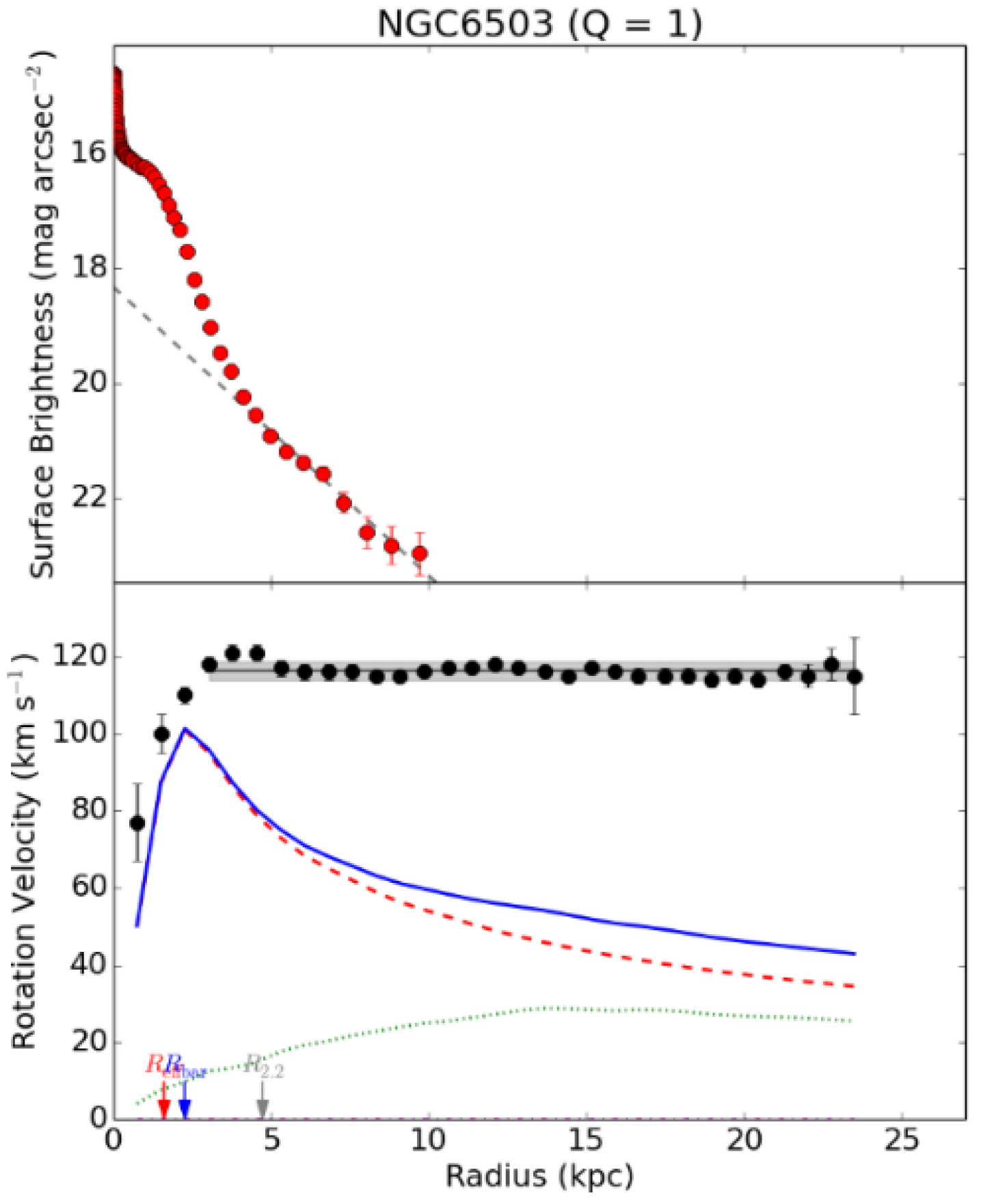
Figure 2.
Two 3D spaces, wxy and wxz, filling a 4D space as a fine fabric with resolution Lp and thickness equal to the GUT-scale, depicted as strings protruding from the plane.
Figure 2.
Two 3D spaces, wxy and wxz, filling a 4D space as a fine fabric with resolution Lp and thickness equal to the GUT-scale, depicted as strings protruding from the plane.
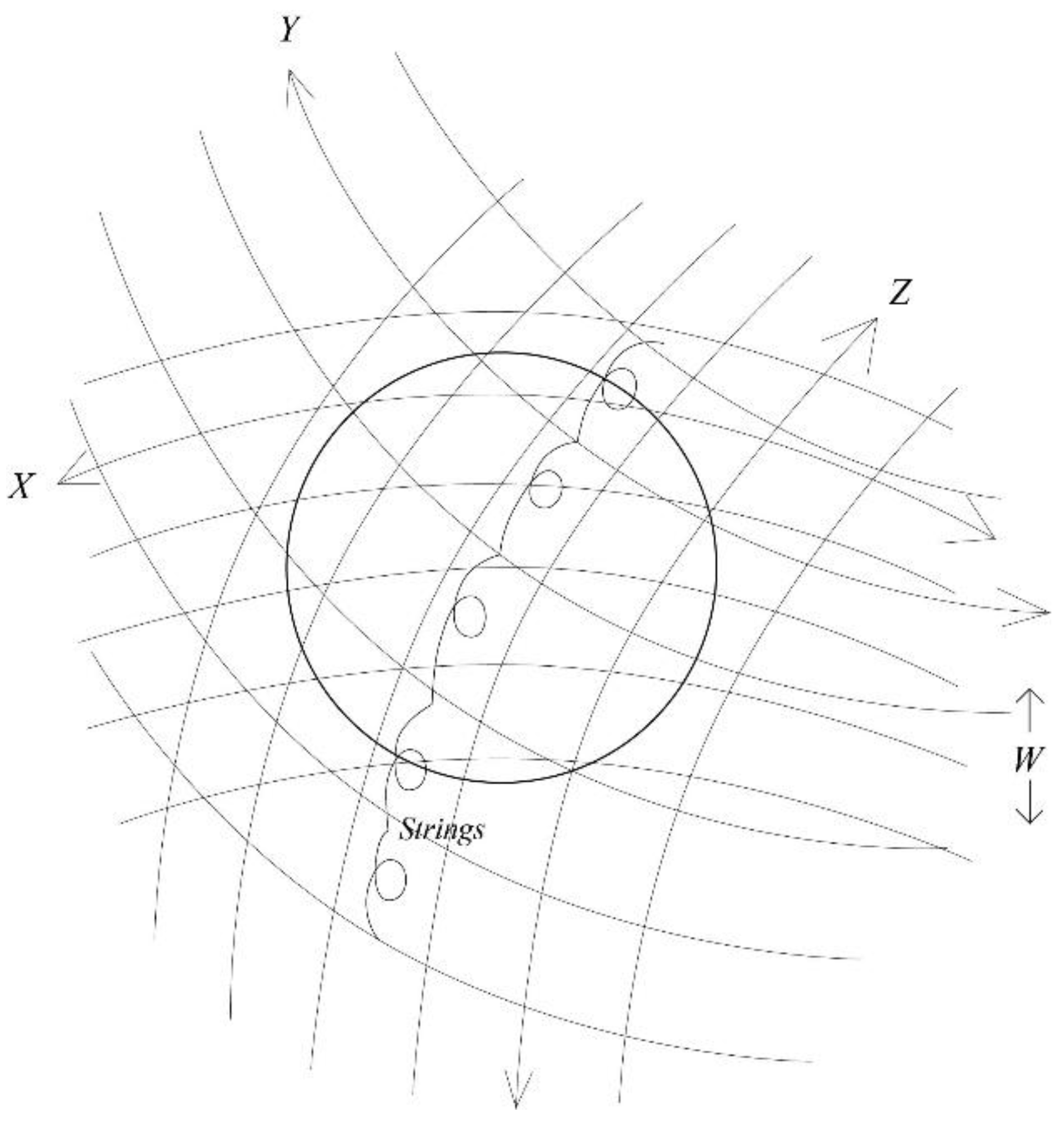
Figure 3.
Compactification of fourth dimension to GUT-scale giving a largely stretched projection of a galaxy or cluster in another universe.
Figure 3.
Compactification of fourth dimension to GUT-scale giving a largely stretched projection of a galaxy or cluster in another universe.
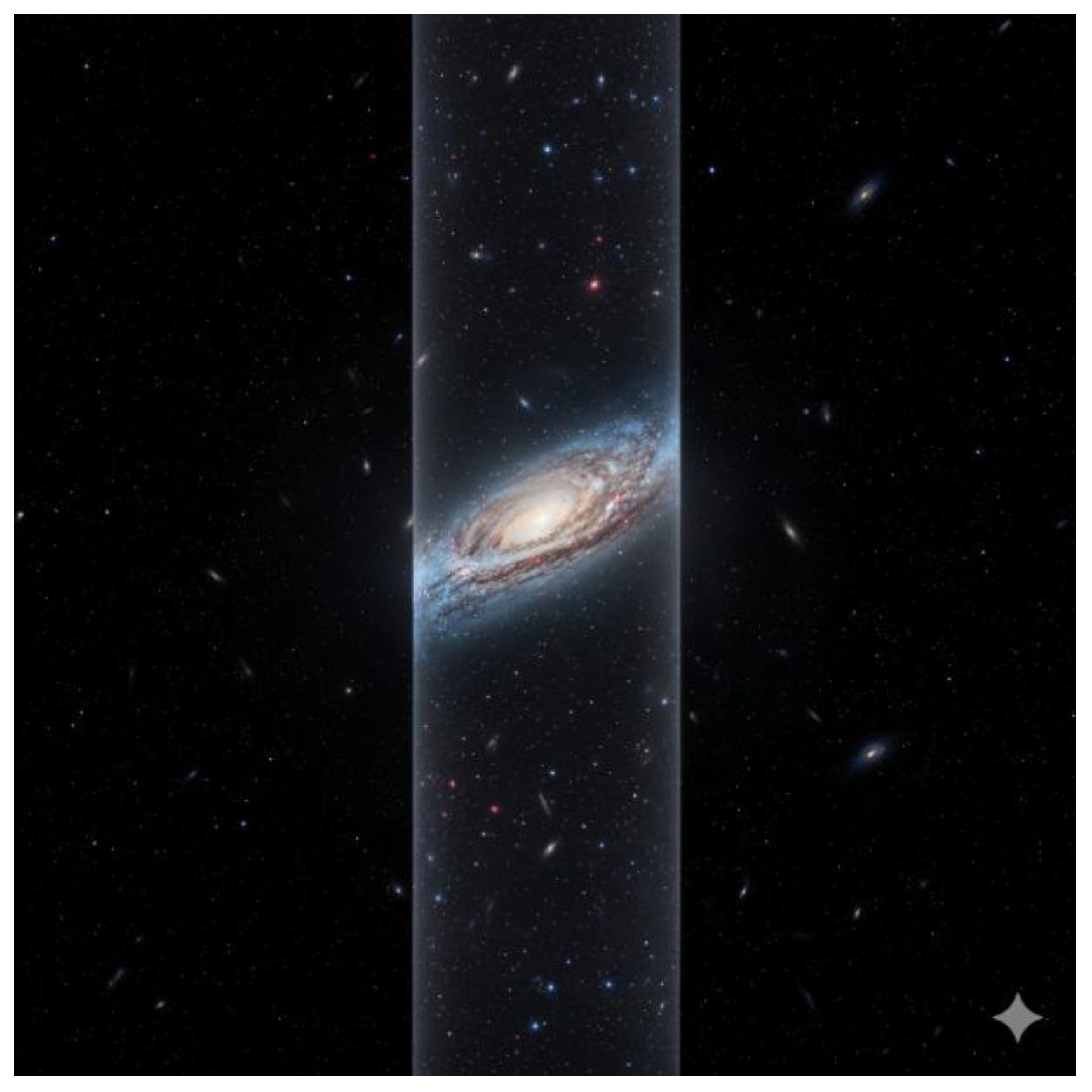
Figure 4.
Vertical disk scale length vs. Vobs after de Kregel et al [44].
Figure 4.
Vertical disk scale length vs. Vobs after de Kregel et al [44].
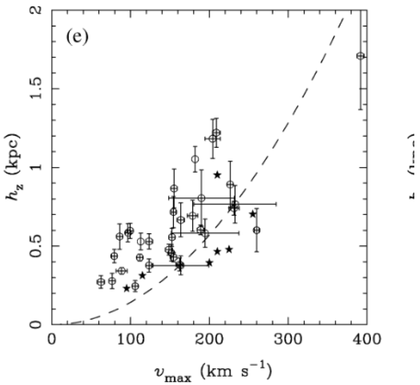
Figure 5.
Vgas, Vdisk and Vbulge from SPARC team and from author assuming mass-light-ratio Yml = 1 (a) UGC11914; (b) UCG09037; the complete figure set of 175 figure is available in Annex 1.
Figure 5.
Vgas, Vdisk and Vbulge from SPARC team and from author assuming mass-light-ratio Yml = 1 (a) UGC11914; (b) UCG09037; the complete figure set of 175 figure is available in Annex 1.
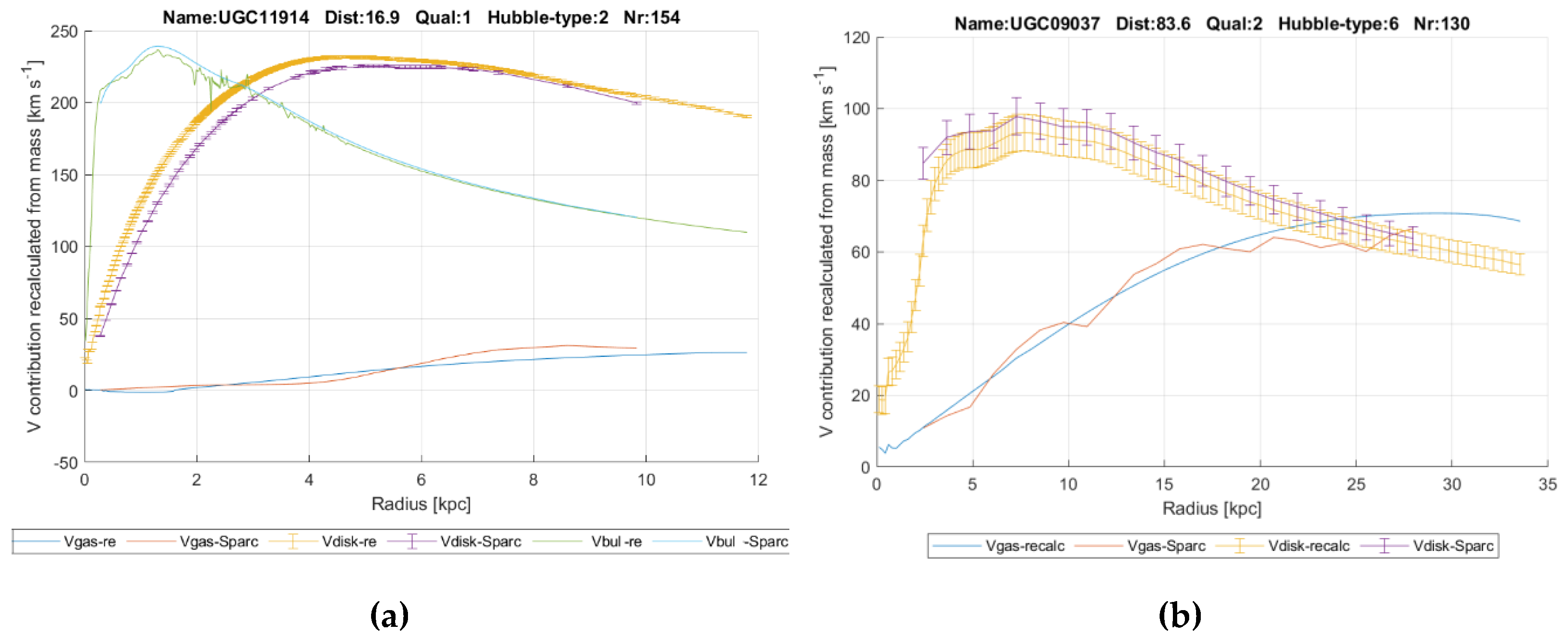
Figure 6.
Example of Vbar from SPARC team and from author with fitted mass-to-light ratio, Yml; the complete figure set of 175 figure is available in Annex 3.
Figure 6.
Example of Vbar from SPARC team and from author with fitted mass-to-light ratio, Yml; the complete figure set of 175 figure is available in Annex 3.
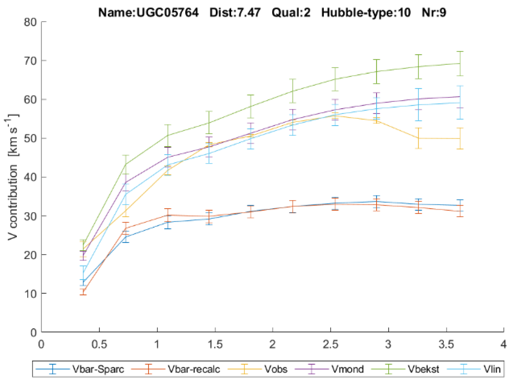
Figure 7.
Disk scale length ratio from de Grijs [50].
Figure 7.
Disk scale length ratio from de Grijs [50].
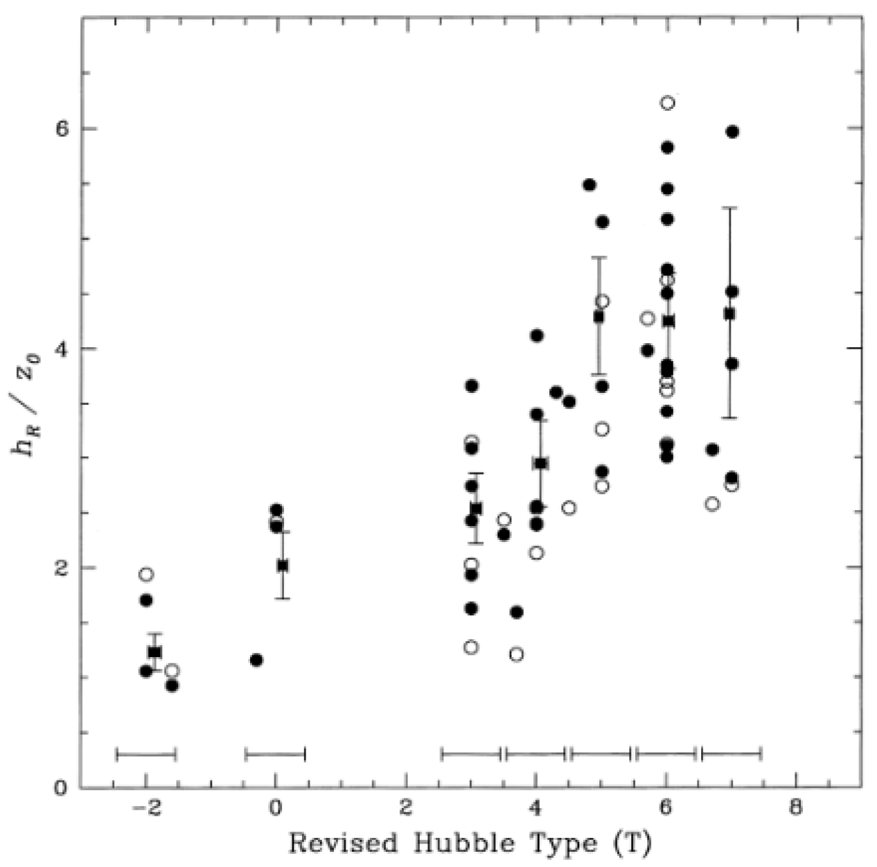
Figure 8.
GL as function of radius in galaxy examples (a) NGC6503; (b) UGC09133; the complete figure set of 175 figure is available in Annex 2.
Figure 8.
GL as function of radius in galaxy examples (a) NGC6503; (b) UGC09133; the complete figure set of 175 figure is available in Annex 2.
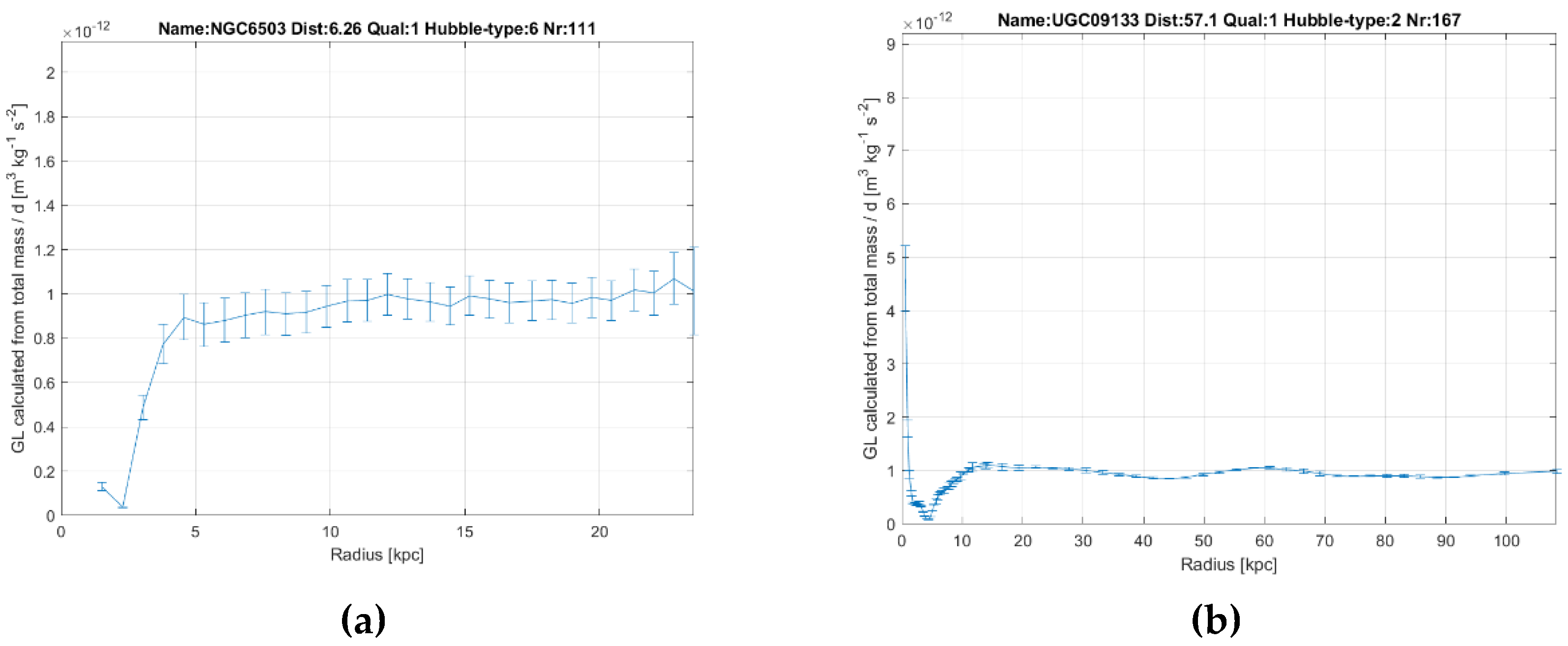
Figure 9.
GL for all 175 galaxies.
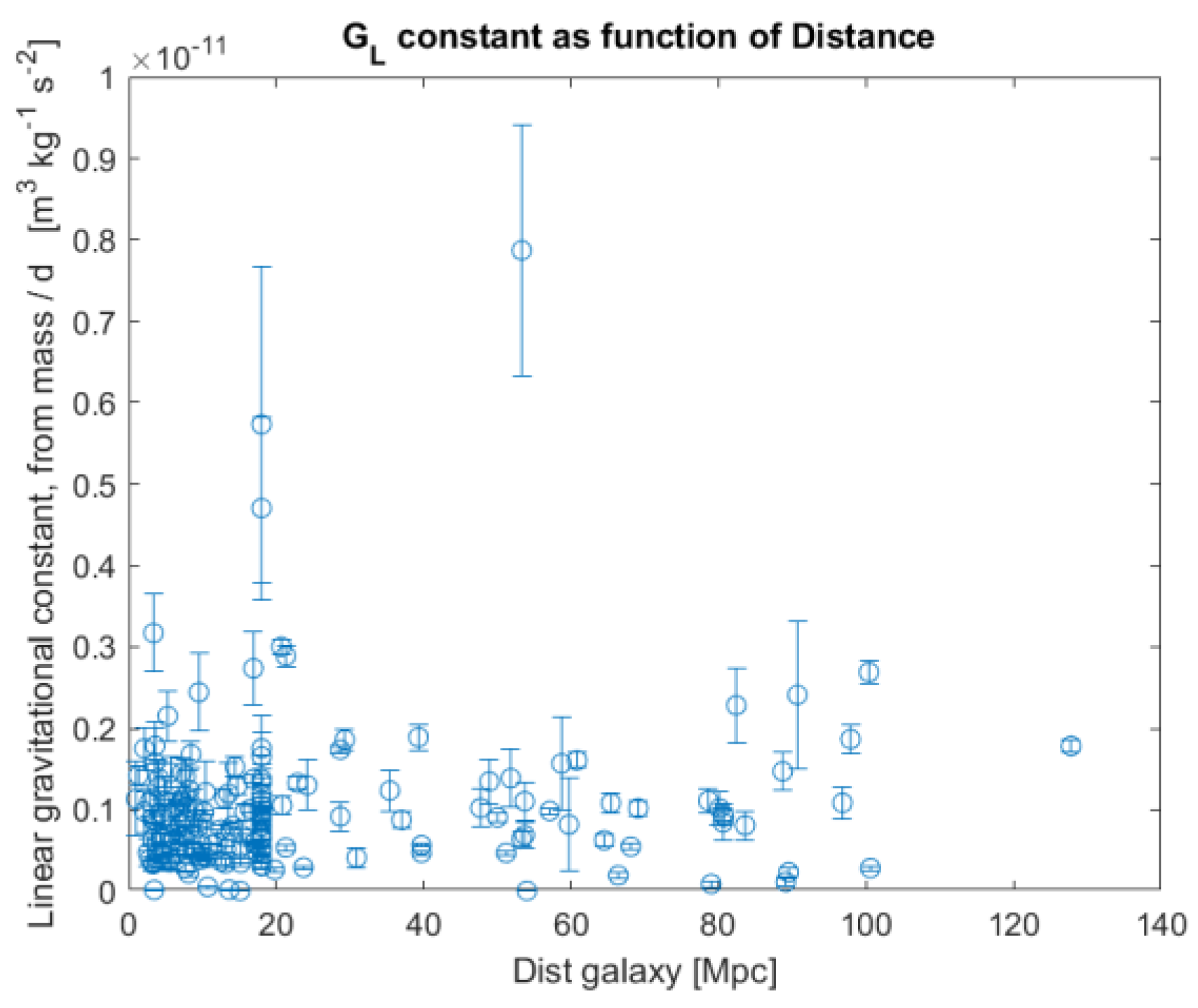
Figure 10.
Predicted over observed gravitational acceleration for 175 galaxies vs. distance to ourselves.
Figure 10.
Predicted over observed gravitational acceleration for 175 galaxies vs. distance to ourselves.
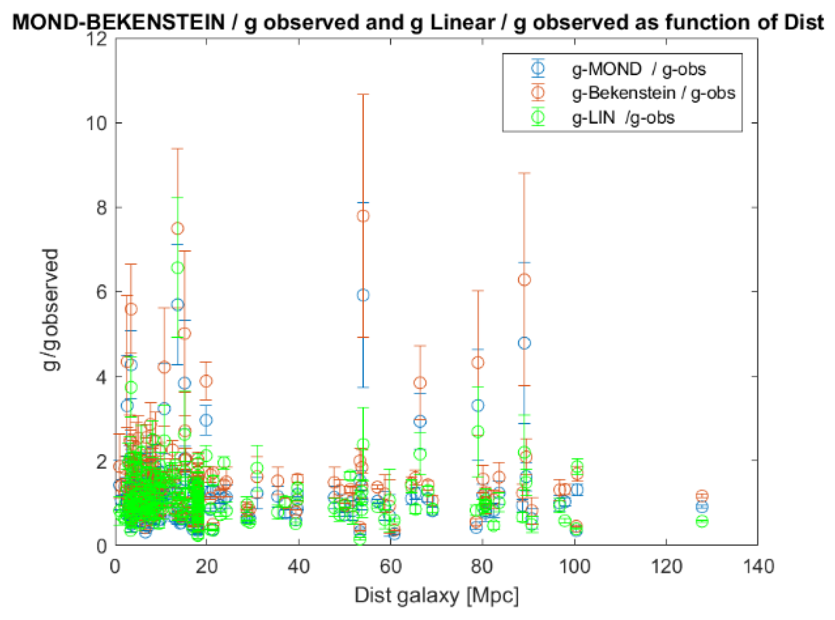
Figure 11.
Examples of rotation curves with MOND, TeVeS and linear gravity predictions; (a) UGC09133, (b) NGC 6503; the complete figure set of 175 figure is available in Annex 3.
Figure 11.
Examples of rotation curves with MOND, TeVeS and linear gravity predictions; (a) UGC09133, (b) NGC 6503; the complete figure set of 175 figure is available in Annex 3.
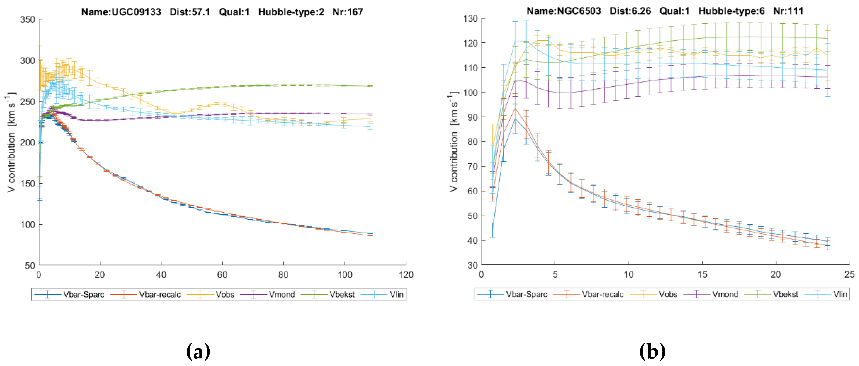
Figure 12.
Velocity dispersions in NGC and Abell clusters as function of cluster mass.
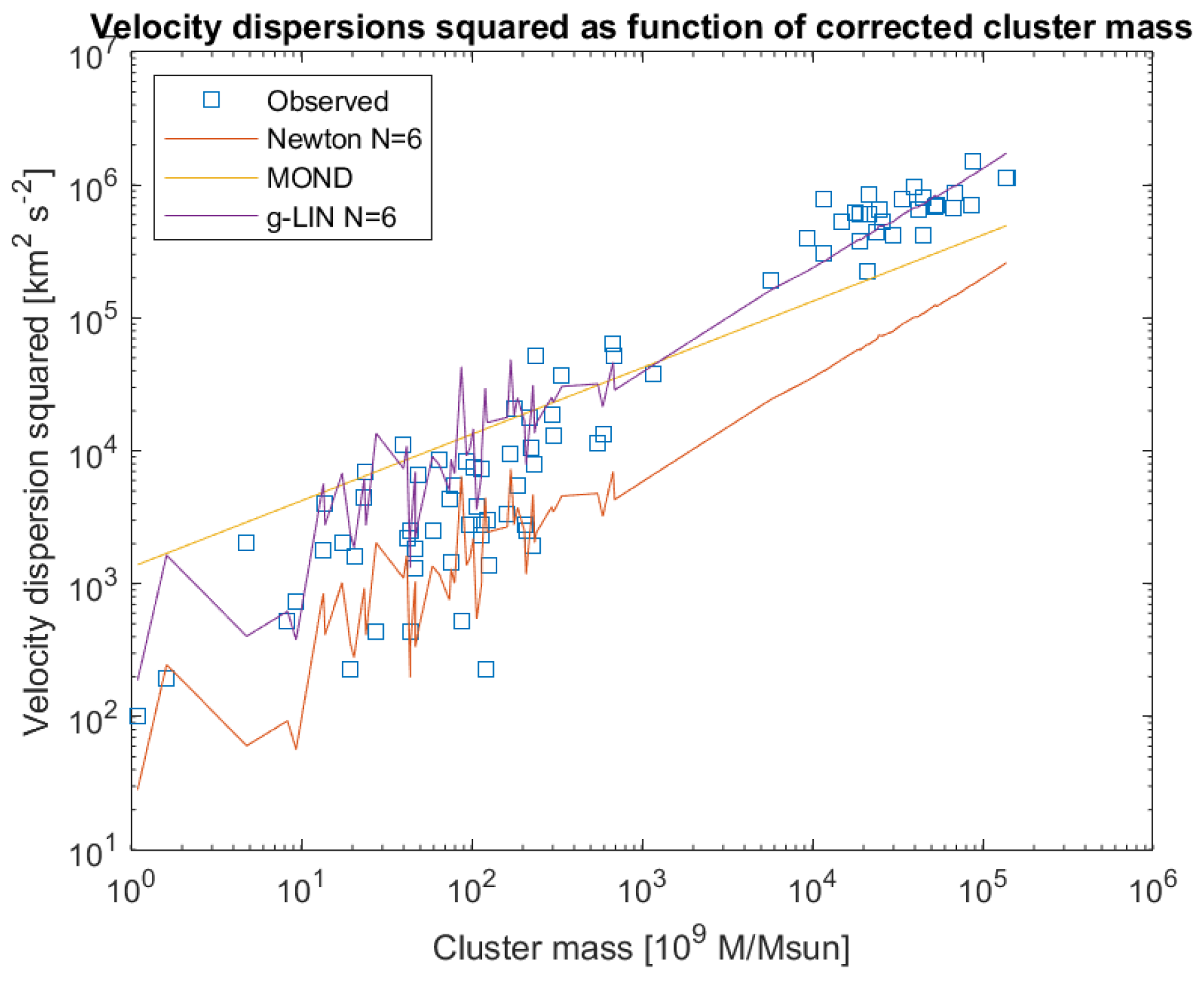
Figure 13.
Early-stage large galaxies from (composed from figures from Labbé et al. 2023) (original source: NASA/ESA/CSA Public Domain).
Figure 13.
Early-stage large galaxies from (composed from figures from Labbé et al. 2023) (original source: NASA/ESA/CSA Public Domain).
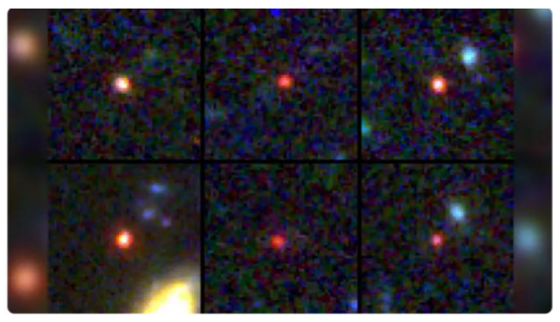
Figure 14.
Dark matter halo orientation, revealing coordinate system of our universe? (source Melissa Weiss/Center for Astrophysics | Harvard & Smithsonian, through Nu.nl).
Figure 14.
Dark matter halo orientation, revealing coordinate system of our universe? (source Melissa Weiss/Center for Astrophysics | Harvard & Smithsonian, through Nu.nl).
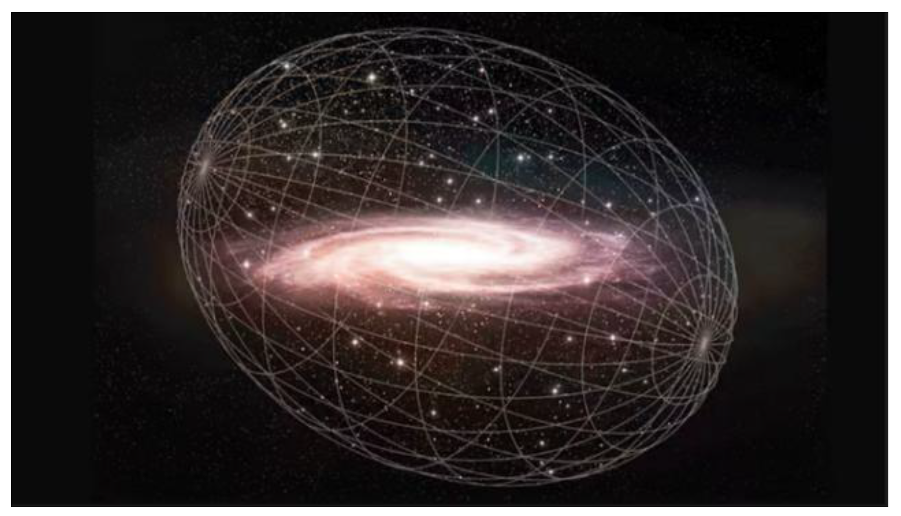

Table 1.
% reduction of deviation prediction-Vobs at all radii [r.m.s. averaged over 175 galaxies], glinear+gbar compared to MOND and TeVeS.
Table 1.
% reduction of deviation prediction-Vobs at all radii [r.m.s. averaged over 175 galaxies], glinear+gbar compared to MOND and TeVeS.
| MOND vs. glinear+gbar | TeVeS vs. glinear+gbar | |
|---|---|---|
| Prediction one GL | 10 % | 17 % |
| Prediction 175 values for GL | 15 % | 22 % |
Table 2.
% reduction of deviation predicted velocity dispersions compared to Newton and MOND.
| Comparison | Newton | MOND |
|---|---|---|
| Prediction logarithmic potential with N = 6 | 57 % | 44 % |
Disclaimer/Publisher’s Note: The statements, opinions and data contained in all publications are solely those of the individual author(s) and contributor(s) and not of MDPI and/or the editor(s). MDPI and/or the editor(s) disclaim responsibility for any injury to people or property resulting from any ideas, methods, instructions or products referred to in the content. |
© 2025 by the authors. Licensee MDPI, Basel, Switzerland. This article is an open access article distributed under the terms and conditions of the Creative Commons Attribution (CC BY) license (http://creativecommons.org/licenses/by/4.0/).
Copyright: This open access article is published under a Creative Commons CC BY 4.0 license, which permit the free download, distribution, and reuse, provided that the author and preprint are cited in any reuse.


