Revisions of the Phenomenological and Statistical Statements of the Second Law of Thermodynamics

1. Introduction

1.1. General Review

The Second Law of Thermodynamics is one of the most remarkable physical laws for its profound meaning, its deep implications in every field of physics and for the several applications in other fields of science such as any field of engineering, chemistry, biology, genetics, medicine and, more generally, in natural sciences.

In simple terms, according to the first Clausius statement (Clausius I statement) the Second Law of Thermodynamics states that the transfer of heat from a higher-temperature reservoir to a lower-temperature reservoir is spontaneous and continue until thermal equilibrium is established. Instead, the transfer of heat from a lower-temperature reservoir to a higher-temperature reservoir is not spontaneous and occurs only if work is done. More profoundly, the understanding of heat and energy and their interplay requires the knowledge of both the First Law of Thermodynamics and the Second Law of Thermodynamics [44].

Thanks to the introduction of the concept of entropy S by Clausius studying the relation between heat transfer and work as a form of heat energy it can be stated a second form of the Second Law of Thermodynamics which can be identified with the second Clausius statement (Clausius II statement) for closed and isolated thermodynamic systems subjected to reversible processes in terms of entropy change: entropy does not decrease, namely $\Delta S\le 0$. Entropy variation $\Delta S$ is equal to the ratio of heat Q reversibly exchanged with the environment and the thermodynamic temperature T at which this exchange occurs, viz. $\Delta S=\Delta Q/T$. If the heat is absorbed from the environment by the thermodynamic system it is $\Delta Q>0$ leading to $\Delta S>0$, while if it is released by the system to the environment it is $\Delta Q<0$. Here, $\Delta$ indicates the finite variation experienced either by entropy or by heat when the thermodynamic system passes from its initial to its final state supposed in thermodynamic equilibrium. The relationship between entropy and heat energy in terms of their variations can be regarded as the quantitative formulation of the Second Law of Thermodynamics based on a classical framework [3,4,5,6,7,8]. This relationship has been given by Clausius also in differential form and for reversible processes it is $dS=\delta Q/T$ where $dS$ is the infinitesimal entropy change due to the infinitesimal heat $\delta Q$ reversibly exchanged. It should be emphasized that, while $\delta Q$ is not an exact differential, $dS$ is a complete (exact) differential due to the integrating factor $1/T$ so that S is a function of state depending only on the initial and final thermodynamic states.

An equivalent formulation of the Second Law of Thermodynamics is represented by the Kelvin statement according to which it is not possible to convert all the heat absorbed from an external reservoir at higher temperature into work: part of it will be transferred to an external reservoir at a lower temperature. The roots were laid in [11,12] where are discussed the consequences of Carnot’s proposition that there is a waste of mechanical energy when heat is allowed to pass from one body to another at a lower temperature. This statement has been historically referred to as the Kelvin-Planck statement [10,13]. However, after Kelvin another pioneer of this principle was Ostwald who completed the Kelvin statement by formulating the perpetuum mobile kind II. For this reason, in this paper, we combine the two pioneering contributions referring to the Kelvin-Ostwald statement. The role of Planck was marginal in the formulation of this principle but was mainly focused in its divulgation within the scientific community.

In strict relation with the above mentioned general statements, it can be stated that, according to the Second Law of Thermodynamics, it is impossible to realize a perpetuum motion machine of the second kind or perpetuum mobile kind II able to use the internal energy of only one heat reservoir (see also Section 1.2 for more details).

As a general note, the entity of entropy variations in the Second Law of Thermodynamics applied to isolated thermodynamic systems allows the distinction between reversible processes, ideal processes for which $\Delta S=0$ ($dS=0$), and irreversible processes, real processes for which $\Delta S>0$ ($dS>0$). To study reversible and irreversible thermodynamic processes it is not sufficient to consider the thermodynamic system itself but also its local and nonlocal surroundings defining together with the system what is called the thermodynamic universe [10,13]. It describes the constructive role of entropy growth and makes the case that energy matters, but entropy growth matters more.

At a later time, the Second Law of Thermodynamics has been reformulated mathematically and geometrically still in a classical thermodynamics framework, through the so called Carathéodory’s principle [18] that exists in different formulations appearing in textbooks and articles (see e.g. [10,13]) even though very similar one to the other. Following Koczan [14] Carathéodory’s principle states: "In the surroundings of each thermodynamic state, there are states that cannot be achieved by adiabatic processes". Often this statement has been given without a rigorous proof of equivalence with other formulations but it has been also proved even though not so rigorously that this principle is a direct consequence of Clausius and Kelvin statements [19,20,21]. However, a recent critique of this principle [22] has allowed to know that it received a strong criticism already by Planck and the issue related to its necessity and validity is still an open debate.

Afterwards, the Second Law of Thermodynamics has acquired a more general significance when it has been introduced a statistical physics definition of entropy by Boltzmann and Planck[23,24,25,26,27] and then generalized by the same Boltzmann [30] and by Gibbs [31], an aspect not discussed in [13]. The main advancement contained in the celebrated Boltzmann probabilistic formula proposed within his kinetic theory of gases, $S_{\mathrm{B}}=k_{\mathrm{B}}\ln \mathcal{W}$ with $k_{\mathrm{B}}$ the Boltzmann constant and $\mathcal{W}$ the number of microstates which characterize a gas’s macrostate. This formula was put forward and interpreted later by Planck [29] and is also known as the Boltzmann-Planck relationship: the entropy of a thermodynamic system is proportional to the number of ways its atoms or molecules can be arranged in different thermodynamic microstates. If the occupation probabilities of every microstate are different it can be shown that Boltzmann formula is written in the Gibbs form or Boltzmann-Gibbs form valid also for states far from thermodynamic equilibrium, $S_{\mathrm{G}}=-k_{\mathrm{B}}\sum p_i\ln p_i$ with $p_i$ the probability that microstate i has energy $E_i$ during the system energy fluctuation. It is straightforward to show that the Boltzmann-Gibbs entropy infinitesimal change in a canonical ensemble is equivalent to the Clausius entropy change and, thanks to this equivalence, the Second Law of Thermodynamics is formulated also within a statistical physics approach.

It is important to point out that, very recently, Koczan has shown that Clausius and Kelvin statements are not exhaustive formulations of the Second Law of Thermodynamics if compared to the Carnot more complete formulation [14]. Specifically, it has been proved that the Kelvin principle is a weaker statement (or more strictly non-equivalent) than the Clausius classical principle (Clausius I principle), and the Clausius I principle is a weaker statement than Carnot principle, which can be considered equivalent to Clausius II principle. By indicating the heat absorbed by a heat source at temperature $T_1$ with $Q_1$ ($Q_1>0$) and the work resulting from the conversion of heat with W in the device operating between the heat source and the heat receiver at temperature $T_2$ Carnot principle states that $Q_1/W\le (T_1-T_2)/T_1$ with $Q_1/W$ the efficiency $\eta$: the efficiency of the heat $Q_1$ conversion process to work W in the device operating in the range between $T_1$ and $T_2$ cannot be greater than the ratio of the difference between the two temperatures and the temperature of the heat source. In this paper a criticism is made to Caratheodory’s principle showing that there is not a real equivalence among this principle and Clausius and Kelvin statements of the Second Law of Thermodynamics contrary to what is asserted in texbooks. Particular attention is also paid to the problem of deriving the Second Law of Thermodynamics from statistical physics. It is also reexamined revised and clarified the problem of reversibility and irreversibility in relation to the usual formulation of the Second Law of Thermodynamics in terms of increasing entropy showing that it cannot be always considered a fundamental and elementary law of statistical physics and, in some cases, even not completely true as recently proved via the fluctuation theorem [39,44]. At the same time, it is also proved that the Second Law of Thermodynamics is a phenomenological law of nature working extremely well for describing the behavior of several thermodynamic systems. In this respect, one of the aims of this work is to explain the above mentioned dissonance basing on precise and novel formulations of the Second Law of Thermodynamics.

This paper is organized as follows: in Section 1 are reviewed the basic definitions of phenomenological thermodynamics, the statistical definitions of entropy and the fluctuation theorem. Section 2 is devoted to some general clarifications of the Second Law of Thermodynamics in its purely phenomenological and classical form, while Section 3 deals with some important clarifications of it in statistical physics. Conclusions are drawn in Section 4.

1.2. Basic Definitions of Phenomenological Thermodynamics

A very important concept that led to the formulation of the laws of thermodynamics was perpetuum mobile. However, even in the classical sense, there are several types of them. It is therefore worth clarifying this type terminology now, so that it can be further developed and used effectively in later sections of the article.

Perpetuum mobile is most often understood to mean a hypothetical device that would operate contrary to the accepted laws of physics. Usually by perpetuum mobile we mean a heat engine or a heat machine - so it has the following basic definitions:

Definition 1 (Perpetuum mobile kind 0 and I) "Perpetuum mobile" kind zero is a hypothetical device that moves forever without power, which appears to be free from resistance to motion. This device neither performs work nor emits heat. However, a "perpetual motion" kind one is a hypothetical device that performs work from nothing or almost nothing (it has an efficiency of infinite or greater than 100%).

Sometimes perpetuum mobile kind 0 is referred to as kind III. However, number 0 better reflects the original Latin meaning of the word (from Latin perpetuum mobile=perpetual motion), and number III will be used further. However, in traditional thermodynamics, the greatest emphasis, not necessarily rightly, was placed on number II.

Definition 2 (Perpetuum mobile kind II) "Perpetuum mobile" kind two is a hypothetical lossless operating warm engine with an efficiency of exactly 100%.

It is quite obvious that kind I and II do not exist, but it is not clear that kind 0 cannot exist. For example, the solar system, which has existed in an unchanged form for millions of years, seems to be kind 0 in kinematic terms. Of course, we assume here that the energy of the Sun’s thermonuclear processes does not directly affect the motion of the planets.

Since the First Law of Thermodynamics was recognized historically later than the Second one, we will introduce a special form of the First Law for the needs of the Second Law.

Definition 3 (First Law of Thermodynamics for two heat reservoirs) We consider thermal processes taking place in contact with two reservoirs: a radiator with a temperature of $T_1$ and a cooler with a temperature of $T_2<T_1$. We will denote the heat released by the radiator by $Q_1$ and the heat absorbed by the cooler by $Q_2$. We assume that we can only transfer work $W\ge 0$ to the environment or absorb work $W\le 0$, but we cannot remove or absorb heat from the environment. Therefore, the principle of conservation of energy for the process takes the form:

$$Q_1=Q_2+W,$$

(1)

which can be written, following the example of the First Law of Thermodynamics, as an expression for the change in the internal energy E of the system:

$$\Delta E=-Q_1+Q_2=-W.$$

(2)

In the set of processes, all possible signs and zeros are allowed for the quantities $Q_1,Q_2,W$ that meet the condition (1) or (2). In addition, thermodynamic processes can be combined (added), but not necessarily subtracted.

The specific form of the First Law of Thermodynamics for a system of two reservoirs results from the assumption of only internal heat exchange. The definition of the first law formulated in this way creates a space of energetically allowed processes for the second law. However, the second rule introduces certain restrictions on these processes (see [14]).

Definition 4 (Clausius First Statement) Heat naturally flows from a body at a higher temperature to a body at a lower temperature. Therefore, a direct (not forced by work) process of heat transfer from the body at a lower temperature to the body at a higher temperature is not possible. Clausius First Principle allows for a large set (sets) of possible physical processes, the addition of which does not violate the above rule or the First Law of Thermodynamics.

Definition 5 (Kelvin–Ostwald Statement) The processes of converting heat to work and work to heat do not run symmetrically. A full conversion of work to heat (internal energy) is possible. However, a full conversion of the heat to the work is not possible in a cyclical process. In other words, there is no Perpetuum Mobile Second Kind. The Kelvin–Ostwald principle allows for the existence of a large set (sets) of possible physical processes, the addition of which does not create a Perpetuum Mobile Second Kind and does not violate the First Law of Thermodynamics.

To provide a more comprehensive statement of the second law of thermodynamics, thermodynamic entropy must be defined. It turns out that this can be done in thermodynamics in three subtly different ways. We will see further that in statistical mechanics, contrary to appearances, there are even more possibilities.

Definition 6 (C-type Entropy for Reservoirs) There is a thermodynamic function of the state of a system of two heat reservoirs. Its change is equal to the sum of the ratio of heat absorbed by these reservoirs to the absolute temperature of these reservoirs:

$$\Delta S_{\mathrm{C}}={\displaystyle \frac{-Q_1}{T_1}}+{\displaystyle \frac{Q_2}{T_2}}.$$

(3)

The minus sign results from the convention that a reservoir with a higher temperature $T_1$ releases heat (for $Q_1>0$). However, if $Q_1<0$, then under the same convention, the reservoir with temperature $T_1$ will absorb heat.

In this version, the total entropy change of the heat reservoirs is considered. We assume that the devices operating between these reservoirs operate cyclically, so their entropy should not change. The definition of type C entropy assumes that the heat capacity of the reservoirs is so large that the heat flow does not change their temperatures. Following Clausius, we can of course generalize the definition of entropy to processes with changing temperature:

Definition 7 (Q-type Clausius Entropy) The entropy change of a thermodynamic system or part of it is the integral of the heat gain divided by the temperature of that system or part of it:

$$\Delta S_Q=\int {\displaystyle \frac{\delta Q}{T}}.$$

(4)

It turns out that in certain irreversible processes, entropy increases despite the lack of heat flow. Therefore, we can further generalize the entropy formula, e.g. for the expansion of gas into a vacuum [15]:

Definition 8 (V-type Entropy) The entropy change of a gas is equal to the integral of the sum of the increase in internal energy and the product of the pressure and the increase in volume divided by the temperature of the gas:

$$\Delta S_V=\int {\displaystyle \frac{dE+pdV}{T}}.$$

(5)

Entropies of type V and Q seem apparently equal, but it will be shown below that this need not be the case - which also applies to entropy of type C. However, for any entropy (by default type C or Q) the following are considered the most popular statement of the second law of thermodynamics (see [14]):

Definition 9 (Clausius Second Statement) There is a function of the state of the thermodynamic system called entropy, which the dependence of the value on time allows to determine the system’s following of the thermodynamic equilibrium. Namely, in thermally insulated systems, the only possible processes are those in which the total entropy of the system (two heat reservoirs) does not decrease:

$$\Delta S_{\mathrm{C}}=\Delta S_1+\Delta S_2\ge 0(\Delta S_Q\ge 0).$$

(6)

For reversible processes, the increase in total entropy is zero, and for irreversible processes it is greater than zero. The same principle can also be applied to Q-type or V-type entropy for a gas system. Then the additivity of entropy for the components of the system must also be respected.

Assuming a given definition of entropy and thanks to the principle of its additivity, the Clausius Second Statement is a direct condition for every process (possible and impossible). Therefore, this principle immediately states which process is possible and which is impossible and should be rejected according to this principle.

However, Clausius First Statement and Kelvin-Olstwald Statement allow us to reject only some of the impossible processes. We reject the remaining part of the impossible processes on the basis of adding processes leading to the impossible ones. Possible processes are those which, as a result of arbitrary addition, do not lead to impossible processes. It has been shown that the Clausius Second Statement is stronger and not equivalent to the Clausius Fist Statement and the Kelvin-Ostwald Statement. [14].

1.3. A Review of Statistical Definitions of Entropy and Application to Ideal Gas

It is also worth considering statistical definitions of entropy. Contrary to appearances, this issue is not disambiguated in relation to phenomenological thermodynamics. On the contrary, there are many different aspects and cases of entropy in statistical physics. It is probably not even possible to talk about a strict universal definition, but only about definitions for characteristic types of statistical systems. Most often, definitions of entropy in statistical physics refer implicite to an equilibrium situation - that is, a state with the maximum possible entropy. From the point of view of the analysis of the second law of thermodynamics, this situation seems loopy - we postulate entropy maximization, but we define maximum entropy. However, dividing the system into subsystems makes sense of such a procedure. This shows a sample of the problem of defining entropy and the problem of precisely formulating the second law of thermodynamics. Boltzmann’s general definition is considered to be the first historical static definition of entropy:

Definition 10 (General Boltzmann entropy for number of microstates) Entropy of the state of a macroscopic system is a logarithmic measure of the number of microstates $\mathcal{W}$ that can realize a given macrostate, assuming a small but finite resolution of distinguishing microscopic states (in terms of location in the volume and values of speed, energy or temperature):

$$S_B:=k_{B}ln\mathcal{W},$$

(7)

where the proportionality coefficient is Boltzmann’s constant $k_B$. The counting of states in quantum mechanics is arbitrary in the sense that it depends on the sizes of the elementary resolution cells. However, due to the property of the logarithm function for large numbers, the resolution parameters should only affect the entropy value in an additive way. In the framework of quantum mechanics, counting states is more literal, but for example, for an ideal gas without rotational degrees of freedom it should lead to essentially the same entropy value.

However, the entropy defined in this way cannot be completely unambiguous as to the additive constant. Even in quantum mechanics, not all microstates are completely quantized, so there must be an element of arbitrariness in the choice of resolution parameters. Even if the quantum mechanics method for an ideal gas were unambiguous, it should be realized that at low temperatures such a method loses its physical sense and cannot be consistent with experiment. Therefore, to eliminate the freedom of constant additive entropy, the third law of thermodynamics is introduced, which postulates zeroing of entropy as the temperature approaches zero. However, such a principle has only a conventional and definitional character and cannot be treated as a fundamental solution - and should not even be treated as a law of physics. Moreover, it does not apply to an ideal gas because no constant will eliminate the logarithm singularity at zero temperature.

Sometimes in the definition of Boltzmann entropy other symbols are used instead of $\mathcal{W}$: $\mathrm{\Omega },\left|\mathrm{\Omega }\right|$ or $\omega$. However, the use of the Greek letter omega may be misleading because it suggests a reference to all microstates of the system, not just those that realize a given macrostate. Therefore, in this article it was decided to use the letter $\mathcal{W}$, just like on Boltzmann’s tombstone - but in a decorative version to distinguish it from the work symbol W.

Until we specify what microstates we consider to realize a given macrostate, then: (i) we do not even know whether we can count microstates of the non-equilibrium type in the entropy formula. Similarly, it is not clear: (ii) can Botzmann’s definition apply to non-equilibrium macrostates? Regarding problem (ii), it seems that the Boltzmann definition can be used for non-equilibrium states, even though the equilibrium entropy formulas are most often given. The latter results from the simple fact that the equilibrium state is described by fewer parameters. For example, when specifying the parameters of the gas state, we mean (consciously or not) the equilibrium state. Therefore, consistently regarding (i), if we have a non-equilibrium macrostate, then its entropy must be calculated after the non-equilibrium microstates. If the macrostate is in equilibrium, it is logical to count the entropy after the microstates relating to equilibrium. Unfortunately, some definitions of entropy force the counting of non-equilibrium states. This is the case, for example, in the microcanonical complex, in which one should consider a state in which one particle has taken over the energy of the entire system. Fortunately, this condition has a negligible importance (probability), so problem (i) is not critical. This is because probability, the second law of thermodynamics, and entropy distinguish equilibrium states. However, this distinction is a result of the nature of things and should not be put into place by hand at the level of definition.

It is worth making the definition of Boltzmann entropy a bit more specific. Let us consider a large $N\ge N_A$ set of identical particles (but not necessarily quantum indistinguishable). Let us assume that we recognize a given macrostate as a specific filling of k cells into which the phase space has been divided (the space of positions and momenta of one particle - not to be confused with the full configuration space of all particles). Each cell contains a certain number of particles, e.g. in the ith cell there are $n_i\ge 0$ particles. Of course, the number of particles must sum to N:

$$n_1+n_2+n_3+...+n_k=N.$$

(8)

Now the possible number of all configurations is equal to the number of permutations with repetitions, because we do not distinguish permutations within one cell:

$$\mathcal{W}={\displaystyle \frac{N!}{n_1!n_2!n_3!...n_k!}}.$$

(9)

In mathematical considerations, one should be prepared for a formally infinite number of cells k and, consequently, fractional or even smaller than unity values of $n_i$. However, even in such cases it is possible to calculate a finite number of states $\mathcal{W}$. Taking the above into account, let’s define the Boltzmann entropy in relation to the Maxwell-Boltzmann distribution:

Definition 11 (Boltzmann entropy at a specific temperature) The entropy of an equilibrium macroscopic system with volume V and temperature T, composed of N "point" particles, is a logarithmic measure of the number of microstates $\mathcal{W}$ that can realize this homogeneous macrostate assuming small volume cells in the space of positions υ and the space of momentum μ:

$$S_{BT}:=k_{B}ln{\mathcal{W}}_{\upsilon ,\mu }(N,V,T),$$

(10)

where the proportionality coefficient is Boltzmann’s constant $k_B$. The counting of states within classical mechanics is arbitrary here, in the sense that it depends on the volume $\upsilon ,\mu$ of the unit cells. However, thanks to the property of the logarithm function for large numbers, these parameters only affect the additive entropy constant (and also allow the arguments of the logarithmic function to be written in dimensionless form).

An elementary formula for this type of Boltzmann entropy can be derived using the formula (9) for the distribution in space cells and the Maxwell-Boltzmann distribution for momentum space (the temperature-dependent part) [32,33]:

$$S_{BT}\approx N{k}_{B}ln{\displaystyle \frac{V}{\upsilon }}+{\displaystyle \frac{3}{2}}N{k}_{B}ln{\displaystyle \frac{T}{\tau }}+{\displaystyle \frac{3}{2}}N{k}_B+\mathrm{const}(N,\upsilon ,\mu ),$$

(11)

where the cell size of the shoot space has been replaced for simplicity by the equivalent temperature "pixel":

$$\tau ={\displaystyle \frac{{\mu }^{2/3}}{3k_{B}m}},$$

(12)

where m is the mass of one particle.

In the formula (11), what is disturbing is the presence of an extensive variable V in the logarithm, instead of an intensive combination of variables $V/N$. In the [32,33] derivation, division by N does not appear implicitly via an additive constant either. The question is whether it is an error of this type of derivation (in two sources) or an error of the definition, which should, for example, include some dividing factor of the Gibbs type? This issue is taken up further in this work. However, it is worth seeing that in the volume part the formula (11) for $2{\mathrm{m}}^3$ of air gives an entropy more than twice as large as for $1{\mathrm{m}}^3$ – and it shouldn’t be like that.

The second doubt concerns the coefficient $3/2$ in the expression $N{k}_B$ in the derivations of [32,33], which also appears in the entropy derived by Sackur in 1913 (see [34]). In further alternative calculations the ratio is $5/2$ – e.g. in Tetrode’s calculations of 1912 (see [34]). It is worth adding that we are considering here a gas of material "points" (so-called monatomic) with the number of degrees of freedom for a determinate particle of 3, not 5. It is therefore difficult to indicate the reason for the discrepancy and to determine whether it is important due to the frequent omission of the considered term (or terms conditioned by "random" constants). There is quite a popular erroneous opinion that the considered term can only be derived on the basis of statistical mechanics, and it cannot be done within the framework of phenomenological thermodynamics. Namely, if, at a constant volume, we start to increase the number of particles with the same temperature, then, according to the definition of the V type, we will obtain the entropy term under consideration with the coefficient $3/2$. However, if the same were calculated formally at constant pressure, the coefficient would be $5/2$.

A steady-temperature state subject to the Maxwell-Boltzmann distribution is effectively a canonical ensemble – this will be analyzed further in these terms. One can also consider a microcanonical ensemble in which the energy E of the system is fixed. This leads to a slightly different way of understanding Boltzmann entropy:

Definition 12 (Boltzmann Entropy at a Specific Energy) The entropy of a macroscopic system with volume V and energy E, composed of N particles, is a logarithmic measure of the number of microstates $\mathcal{W}$ that can realize this homogeneous macrostate assuming small cells of volume υ and low resolution of energy levels ε:

$$S_{BE}:=k_{B}ln{\mathcal{W}}_{\upsilon ,\epsilon }(N,V,E),$$

(13)

where the proportionality coefficient is Boltzmann’s constant $k_B$. The counting of states within classical mechanics is arbitrary in the sense that it depends on the choice of the size of the elementary volume cell and the choice of the width of the energy intervals. However, due to the property of the logarithm function for large numbers, the parameters υ and ε only affect the entropy value in an additive way.

The calculation of this type of Boltzmann entropy for a part of the spatial volume is the same as before. Unfortunately, calculating the energy part is much more difficult. First, one must consider the partition of energy E into individual molecules. Secondly, the isotropic velocity distribution should be considered here without assuming the Maxwell-Boltzmann distribution. Therefore, the counting of states should take place over a larger set than for equilibrium states, but for states that are isotropic in terms of velocity distribution.

Counting states using the partition function is rarely performed because it is cumbersome. An example is the calculations for the photon sphere of a black hole in the context of Hawking radiation [15]. These calculations resulted in a result consistent with the equation of state of the photon gas, but compliance with Hawking radiation was obtained only for low energies.

While the Boltzmann entropy of the $S_{BT}$ type was defined directly for equilibrium states, and the entropy of the $S_{BE}$ type counted isotropic, but not necessarily equilibrium, states, one can also consider the entropy counting even non-isotropic states. This takes place in the extended phase space, i.e. in the configuration space, where the state of the microstate is described by one point in the $6N$ space. Namely, there is another approach to measuring the complexity of a macrostate from previous ones. Instead of dividing the space of positions and pedos into cells and counting all possibilities, we can take as a measure the volume of configurational phase space that a given macrostate could realize. Unfortunately, energy resolution or cell size is also somewhat useful here.

Definition 13 (Boltzmann Entropy for a Phase Volume with the Gibbs Factor) The entropy of a macroscopic system with a volume V, composed of N particles, is a logarithmic measure of the phase volume $\overline{\Gamma }·\epsilon$ of all microstates of the system with energy in the range $(E,E+\epsilon )$, which can realize a given macrostate with energy in this range:

$$S_{\Gamma }:=k_{B}ln{\displaystyle \frac{\overline{\Gamma }(N,V,E)·\epsilon }{N!\omega }}=:k_{B}ln{\displaystyle \frac{{\mathcal{W}}_{\Gamma }}{N!}},$$

(14)

where, in addition to the unit volume of the ω phase space configuration cell, the so-called Gibbs divisor $N!$. The role of the Gibbs divider is to reduce a significant value of the phase volume and is sometimes interpreted on the basis of the indistinguishability of identical particles. The dependence on the parameters ε and ω is additive.

The definition could be limited to the surface area $\Gamma$ of the hypersphere in the configurational phase space instead of the volume $\overline{\Gamma }·\epsilon$ of the hypersphere shell. This would remove the $\epsilon$ parameter, but would formally require changing the volume of the unit cell to a unit area one dimension smaller.

In Boltzmann phase entropy, counting takes place over all microstates from the considered energy range. Therefore, both non-isotropic states in velocity and non-uniform states in position - in short, non-equilibrium states - are taken into account. Nevertheless, we will refer the entropy to the equilibrium state, since no non-equilibrium parameters are given for the state. The entropy of non-equilibrium macrostates can be found by dividing them into subsystems that can be treated as equilibrium, and then adding their entropies.

It is often postulated that the volume of a unit cell in phase space follows from the Heisenberg uncertainty principle ${\sigma }_x{\sigma }_{p_x}\ge \hslash /2$. Then it should be $\omega ={(\hslash /2)}^{3N}$, although it is usually simplified to $\omega =h^{3N}$, because units are more important than values (however, the problem of the presence of a divisor $4\pi$ is decidable in quantum computations). However, if the size of the unit cell approached zero, the entropy would approach infinity.

The area of the constant energy phase hypersurface of dimension $6N-1$ can be calculated from the exact formula for the area of an odd-dimensional hypersphere of radius r immersed in an even-dimensional space:

$$A_{6N-1}=V^N{A}_{3N-1}\left(r\right),$$

(15)

$$A_{3N-1}\left(r\right)={\displaystyle \frac{2{\pi }^{3N/2}}{\Gamma (3N/2)}}{r}^{3N-1}.$$

(16)

Taking into account that the radius of the sphere in the configurational momentum space can be related to the energy for material points $r=p=\sqrt{2mE}$ as follows, we obtain:

$${\displaystyle \frac{{\mathcal{W}}_{\Gamma }}{N!}}={\displaystyle \frac{\overline{\Gamma }(N,V,E)·\epsilon }{N!\omega }}={\displaystyle \frac{V^{N}2{\pi }^{3N/2}\epsilon }{N!\Gamma (3N/2)h^{3N}}}{\sqrt{2mE}}^{3N-1}.$$

(17)

For further simplifications, Stirling’s asymptotic formula is standardly used:

$$\Gamma \left(n\right)=(n-1)!\cong \sqrt{2\pi n}{\left({\displaystyle \frac{n}{e}}\right)}^n\approx n!.$$

(18)

Its application to further approximations leads to:

$$lnN!\approx NlnN-N,$$

(19)

$$ln\Gamma (3N/2)\approx {\displaystyle \frac{3}{2}}NlnN-{\displaystyle \frac{3}{2}}N.$$

(20)

On this basis, the Boltzmann phase entropy of an ideal gas takes the form:

$$S_{\Gamma }\approx N{k}_{B}ln{\displaystyle \frac{V}{N\upsilon }}+{\displaystyle \frac{3}{2}}N{k}_{B}ln{\displaystyle \frac{E}{N\epsilon }}+{\displaystyle \frac{5}{2}}N{k}_B+\mathrm{const}(N,m,\epsilon ,h),$$

(21)

where the auxiliary dimensional constant $\upsilon$ was chosen so that the volume of the phase cell of one particle is $\upsilon {\sqrt{2m\epsilon }}^3=h^3$. It is customary to simply omit the dimensional constants and the additive constant (but not in the so-called Sackur-Tetrode entropy formula). In any case, here the simplest part of the additive term has a coefficient of 5/2, and not 3/2 as before. Furthermore, the volume under the logarithm sign is divided by the number N of particles. Generally, the presented result and the derivation method are consistent with the Tetrode method (see [34]).

There is no temperature yet in the entropy formula obtained from the microcanonical decomposition. However, the general formalism of thermodynamics allows us to introduce such a temperature in a formal way:

$${\displaystyle \frac{1}{T}}:={\left({\displaystyle \frac{\partial S}{\partial E}}\right)}_{N,V}\approx {\displaystyle \frac{3}{2}}N{k}_B{\displaystyle \frac{1}{E}}.$$

(22)

The formula uses the phase Boltzmann entropy $S_{\Gamma }$, although the formula also applies to the entropy $S_{BE}$, which, however, has not been calculated (at least here). In any case, using the above relation between temperature and energy, the entropy $S_{\Gamma }$ can be given a form almost equivalent to the entropy $S_{BT}$. The difference concerns the discussed factor dividing the volume and the less important term with factors 5/2 vs 3/2.

There is yet a slightly different approach to the statistical definition of entropy than Boltzmann’s original approach. Most often it refers to the canonical distribution and is attributed to Gibbs. Gibbs was probably the first to use the new formula for statistical entropy, but Boltzmann did not shy away from this formula either (see below). In addition, Shannon used this formula in information theory, as well as in ordinary mathematical statistics without a physical context.

Definition 14 (Gibbs or Gibbs–Shannon entropy) The entropy of a macroscopic system whose microscopic energy realizations have probabilities $p_i$ is given by:

$$S_G=:-k_B\sum _i{p}_{i}ln{p}_i,$$

(23)

where the proportionality coefficient is the Boltzmann constant $k_B$ taken with a minus sign. The counting of states may be arbitrary in the sense of dividing them into micro-scale realizations of a macrostate and, consequently, assigning them a probability distribution.

Gibbs entropy usually applies to a canonical system in which the energy of the system is not strictly defined, but the temperature is specified. Therefore, we can only talk about the dependence of entropy on the average energy value. In a sense, entropy (like energy) in the canonical distribution also has a secondary, resulting role. Well, a more direct role is played by the Helmholtz free energy, which in thermodynamics is defined as follows:

$$F=\langle E\rangle -TS.$$

(24)

Only from this energy can entropy be calculated. This will be an entropy equivalent to the Gibbs entropy, but due to a different way of obtaining it, we will treat it as a new definition:

Definition 15 (Entropy of type F) The entropy of the (canonical) system, expressed in terms of the Helmholtz free energy F, is with the opposite sign equal to the partial derivative of this free energy with respect to temperature:

$$S_F:=-{\left({\displaystyle \frac{\partial F}{\partial T}}\right)}_{V,N}.$$

(25)

In statistical terms, the free energy F is proportional with a sign opposite to the absolute temperature and to the logarithm of the statistical sum:

$$F:=-k_{B}TlnZ.$$

(26)

The statistical sum is the normalization coefficient of the unnormalized exponential probabilities $P_i=p_{i}Z$ of energy in the thermal (canonical) distribution:

$$Z:=\sum _i{P}_i:=\sum _{i}exp\left(-{\displaystyle \frac{E_i}{k_{B}T}}\right).$$

(27)

Although this definition partially resembles the Boltzmann definition (e.g. instead of the number of states $\mathcal{W}$ there is a statistical sum Z), it is more complex and specific (it includes temperature, which complicates the partial derivative). At least superficially, this entropy seems to be slightly different from the general idea of Boltzmann entropy (or even from Gibbs entropy):

$$S_F=k_{B}lnZ+k_{B}T{\left({\displaystyle \frac{\partial lnZ}{\partial T}}\right)}_{V,N}=k_{B}lnZ+{\displaystyle \frac{1}{T}}\langle E\rangle ,$$

(28)

but in a moment we will see that this additional last term contains only a part proportional to the number of particles N and is often omitted in many types of entropy (does not apply to Sackur–Tetrode entropy). However, in this work it was decided to check the main part of this term, omitting the scale constants (Planck’s constant, the sizes of unit cells, the mass of particles, the logarithms of pi and e).

For an ideal gas, the statistical sum Z can be calculated similarly to the calculation of entropy $S_{BT}$. In the case of calculating the Boltzmann entropy $S_{BT}$, we referred to arbitrary cells of the position and momentum space. Due to the discrete nature of the statistical sum, its calculation is usually performed as part of quantization on a cubic or cuboid box. The spatial boundary conditions on the box quantize momentum and energy, so the counting takes place only in terms of momentum quantum numbers - the volume of the box appears only indirectly in these relations. The result of this calculation is [35]:

$$Z={\displaystyle \frac{V^N}{N!h^{3N}}}{\sqrt{2\pi m{k}_{B}T}}^{3N}.$$

(29)

We see that this value is very similar to ${\mathcal{W}}_{\Gamma }/N!$ when calculating the Boltzmann entropy of the type $S_{\Gamma }$. Indeed, after making standard approximations, the first principal term ($k_{B}lnZ$) of the entropy of a perfect gas of the $S_F$ type will differ from the previous entropy only by a term proportional to the variable N itself. However, the additional additive term of this entropy will be $3N{k}_B/2$ and will reconcile these entropies:

$$S_F\approx N{k}_{B}ln{\displaystyle \frac{V}{N\upsilon }}+{\displaystyle \frac{3}{2}}N{k}_{B}ln{\displaystyle \frac{T}{\tau }}+{\displaystyle \frac{5}{2}}N{k}_B+\mathrm{const}(N,m,h,k_B),$$

(30)

where this time the auxiliary dimensional constants $\upsilon$ and $\tau$ satisfy the relation $\upsilon {\sqrt{2\pi m{k}_B\tau }}^3=h^3$.

In addition to the microcanonical and canonical (thermal) systems, there is also a large canonical system in which even the number of particles is not constant. Due to the numerous complications in defining entropy so far, the grand canonical system will not be considered here. Even more so, niche isobaric systems (isothermal or isenthalpic) will be omitted.

Note that the probability appearing in the Gibbs entropy is simply normalized to unity, and not to the number of particles N, which may suggest that the Gibbs entropy differs from the Boltzmann-type entropy in the absence of this multiplicative factor N. Indeed, this is reflected in the next version of Boltzmann entropy, in which there is a single-particle probability distribution function in the phase space [36] normalized to N (and not to unity):

Definition 16 (Boltzmann entropy of H type) In the state described in the phase space by the single-particle distribution function $f(t,\overrightarrow{r},\overrightarrow{v})$, the entropy of the H system (or simply the $-H$ function, but not the Hamiltonian and not enthalpy) is defined by the following logarithm integral:

$$S_H:=-k_B\int f(t,\overrightarrow{r},\overrightarrow{v})ln{\displaystyle \frac{f(t,\overrightarrow{r},\overrightarrow{v})}{e}}{d}^{3}r{d}^{3}v=:-H,$$

(31)

whereby the distribution function is normalized to a number of particles N, and the constant e in the denominator does not have any fundamental character.

Note that the divisor e after taking into account the normalization condition of the distribution function leads to an additive entropy term of $N{k}_B$ without the factors $3/2$ or $5/2$. However, perhaps this divisor actually corrects the target entropy value.

Moreover, it is often assumed that the quantity defined above (or slightly modified) is not entropy, but taken with the opposite sign, the so-called H function. However, in the light of the various definitions cited in this work, there is no point in considering this quantity as something different from entropy. All the more so because Boltzmann formulated a theorem regarding this function, which was supposed to reflect the second law of thermodynamics. To formulate this theorem, the Boltzmann kinetic equation and the assumption of molecular chaos are also needed.

The Boltzmann kinetic equation for the one-particle distribution function $f(t,\overrightarrow{r},\overrightarrow{v})$ of the initial state N postulates that the complete derivative of the distribution function is equal to the partial derivative taking into account two-particle collisions:

$${\displaystyle \frac{df}{dt}}:={\displaystyle \frac{\partial f}{\partial t}}+\overrightarrow{v}·{\displaystyle \frac{\partial f}{\partial \overrightarrow{r}}}+\overrightarrow{g}·{\displaystyle \frac{\partial f}{\partial \overrightarrow{v}}}={\left({\displaystyle \frac{\partial f}{\partial t}}\right)}_{coll},$$

(32)

where $\overrightarrow{g}$ is the external acceleration field – e.g., the gravitational field.

The assumption of molecular chaos (Stosszahlansatz), in simple terms, consists in assuming that two-particle collisions are factored using the one-particle distribution function as follows:

$${\left({\displaystyle \frac{\partial f}{\partial t}}\right)}_{coll}(t,\overrightarrow{r},\overrightarrow{v})=\int d\mathrm{\Omega }\int d^3{v}_1|{\overrightarrow{v}}_1-\overrightarrow{v}|\left(f(t,\overrightarrow{r},{\overrightarrow{v}}_1^{\prime })f(t,\overrightarrow{r},{\overrightarrow{v}}^{\prime })-f(t,\overrightarrow{r},{\overrightarrow{v}}_1)f(t,\overrightarrow{r},\overrightarrow{v})\right){\displaystyle \frac{d\sigma }{d\mathrm{\Omega }}},$$

(33)

where $d\sigma /d\mathrm{\Omega }$ is the differential cross section related to the velocity angles satisfying the relation $|{\overrightarrow{v}}_1-\overrightarrow{v}|=|{\overrightarrow{v}}_1^{\prime }-{\overrightarrow{v}}^{\prime }|$. The kinematic-geometric idea of the molecular chaos assumption is quite simple (it is a simplification), but the mathematical formula itself is already complex - we will not go into details here. It turned out that the assumption Stosszahlansatz together with the evolution equation (32) was enough for Boltzmann, in a sense, to derive the second law of thermodynamics:

Theorem 1 (H Boltzmann) If the single-particle distribution function $f(t,\overrightarrow{r},\overrightarrow{v})$ satisfies the "Stosszahlansatz" assumption regarding the Boltzmann evolution equation (32), then the entropy of the H Boltzmann type is nondecreasing time function:

$${\displaystyle \frac{d{S}_H}{dt}}\ge 0\mathrm{or}\Delta S_H\ge 0.$$

(34)

The proof of Boltzmann’s theorem, in a notation analogous to the one adopted here, can be found in the textbooks [36,37].

Although Boltzmann’s theorem is a true mathematical theorem, it is unfortunately not (and cannot be) a derivation of the second law of thermodynamics. The thesis of every theorem follows from an assumption, and the assumption of molecular chaos (Stosszahlansatz) is not entirely true. This assumption, in some strange way, introduces irreversibility and asymmetries of time evolution into the macroscopic system, when the remaining equations of physics do not contain this element of time asymmetry. This issue has even been called the irreversibility problem or even Loschmidt’s irreversibility paradox.

Typically, in the context of the irreversibility problem, it is claimed (somewhat incorrectly) that all the fundamental equations of physics are time-symmetric. However, this does not in any way apply to equations involving resistances to motion, including friction. It is difficult to explain why the aspect of resistance to motion is so neglected in physics. Ignorance of resistance to movement is imputed to Aristotle, when in fact it is exactly the opposite and Aristotle described the proportion of movement that included resistance. This proportion can even be interpreted as consistent with Newtonian dynamics according to the some corresponding correspondence principle [38]. The time asymmetry of Aristotle’s equation (proportion) of dynamics was noticed by the American physicist Leonard Susskind (see [38]). Another example of an equation lacking time symmetry is the Langevin equation, which relates to friction in statistical mechanics.

In the context of Boltzmann and statistical physics, it is impossible not to mention the very fundamental ergodic hypothesis, which serves as a basic assumption and postulate. The ergodic hypothesis assumes that the average value of a physical quantity (random variable) based on a statistical distribution is realized over time, i.e. it tends to the average time value of this physical quantity (random variable). Let us assume that this pursuit simply boils down to the postulate of equality of these two types of averages (without precisely defining the period $\Delta t$ of this averaging):

$$〈X\left(t\right)〉\stackrel{!}{\approx }{\overline{X\left(t\right)}}_{\Delta t},$$

(35)

$$\sum _i{p}_i\left(t\right)X_i\left(t\right)\stackrel{!}{\approx }{\displaystyle \frac{1}{\Delta t}}{\int }_t^{t+\Delta t}X\left(t^{\prime }\right)d{t}^{\prime }.$$

(36)

If the distribution is stationary (does not evolve over time), then of course $\Delta t$ can and should tend to infinity $+\infty$. And this is indeed the standard assumption - however, averaging over the future or past or the entire timeline should not differ. However, for non-stationary (time-dependent) distributions, averaging over an infinite time seems to be pointless. In such situations, one could therefore consider "local" averages over time. Then the forward time averaging used above could prefer to evolve forward in time relative to the symmetric averaging time interval. Unfortunately, ergodicity is limited to stationary situations, even where it supposedly does not always occur.

As you can see, the physical status of the ergodic hypothesis is not entirely clear. While the left side of the considered equalities has a clear statistical sense, it is not entirely clear how to determine the right side, which requires knowledge of the time evolution of the system under consideration. Namely, what Liouville equation should be used to describe this evolution in time: the Boltzmann equation or some other equivalent? In other words, it is not clear whether in practice the ergodic hypothesis is a working definition of time averages (right-hand side), or whether it is a postulate or principle of physics that can be confirmed or disproved theoretically or experimentally. The literature states as an indisputable fact that given known systems are ergodic or not ergodic. Nevertheless, it seems that in this matter we should be more humble regarding the physical status of the ergodic hypothesis and treat it as an important methodological tool. In any case, it seems that the ergodic hypothesis should be independent of the Botzmann equation with molecular chaos. Therefore, the problem of irreversibility cannot be solved merely by questioning the ergodic hypothesis. Erodicity should not be confused with weak erdodicity, which is based on the Boltzmann equation as a simplifying assumption.

Regardless of the existence of resistance to motion, the criticisms of the molecular chaos assumption, the problems with the status of ergodicity, or Boltzmann’s generally enormous contribution, it seems that the essence of the second law of thermodynamics in a statistical approach can be contained in the newer fluctuation theorem and its corollary, the second-law inequality.

1.4. The Fluctuation Theorems and an Inequality of the Second Law

It is well established in classical thermodynamics that, according to the well-known formulation of the Second Law of Thermodynamics, the entropy of an isolated thermodynamic system tends to increase until it reaches thermodynamic equilibrium. However, bearing in mind the statistical nature of entropy, an aspect not discussed in Ref.[13], recently it has been formulated the so called fluctuation theorem which gives further information not contained in the Second Law of Thermodynamics. This theorem states that there exists a relative probability that the entropy production of an out-of-equilibrium thermodynamic system could fluctuate in time, viz. either $\Delta S_t>0$ or $\Delta S_t<0$: entropy can also decrease [39,44]. The notion of entropy production can be interpreted quasi-mechanically in the context of the Clausius definition (type Q or V) [45]:

Definition 17 (Entropy production) In a system at temperature T, in which particles with a certain distribution of velocities $\overrightarrow{v}$ are subjected to a force $\overrightarrow{F}$ (of an optical nature [45]), the following entropy change occurs after time t:

$$\Delta S_t:={\displaystyle \frac{1}{T}}{\int }_0^t\overrightarrow{v}\left(t^{\prime }\right)·\overrightarrow{F}\left(t^{\prime }\right)d{t}^{\prime },$$

(37)

where we interpret the integral as some kind of mechanical work (equivalent to heat), and not as an averaging over time (after division by t). Similarly, we also do not divide by Boltzmann’s constant in order to preserve the natural physical unit of entropy.

A newer version of the fluctuation theorem has been formulated by Evans et al. [39] for non-equilibrium steady states that are thermostated keeping constant the total energy. Afterwards, Gallavotti and Cohen proved the theorem for chaotic, isoenergetic non-equilibrium systems [40,41]. The fluctuation theorem in its newer version states:

Theorem 2 (Newer Fluctuation theorem) In out-of-equilibrium thermodynamic systems the ratio between the probability that the entropy production $\Delta S_t$ takes the positive value $k_B\sigma$ and the probability that it takes the negative value $-k_B\sigma$, in a time interval t, follows an exponential law and increases of a quantity with increasing σ:

$${\displaystyle \frac{Pr\left(\Delta S_t=k_B\sigma \right)}{Pr\left(\Delta S_t=-k_B\sigma \right)}}=exp\left(\sigma \right),$$

(38)

where, $Pr(\Delta S_t=k_B\sigma )$ or $Pr(\Delta S_t=-k_B\sigma )$, is the probability that $\Delta S_t$ assumes the value $k_B\sigma$ or $-k_B\sigma$ in a time interval t.

The theorem has been demonstrated via computer simulations, for example, by exploring the temporal evolution of the anisotropy in the probability of observing trajectory segments with positive average entropy production and their conjugate trajectory antisegments with negative average entropy production for reversible deterministic systems and for Hamiltonian systems with and without applied dissipative fields.[42,43]. The theorem has also been experimentally proved by observing the time-dependent relaxation of a colloidal particle under a step change in the strength of a stationary optical trap [46].

According to Eq.(38), for a finite thermodynamic system in a time interval t, there is a non-zero probability that the entropy production flows in a direction that is opposite to the one predicted by the Second Law of Thermodynamics. We emphasize that this theorem only apparently contradicts the Second Law of Thermodynamics. Indeed, the fluctuation theorem is valid for both microscopic and macroscopic systems while the Second Law of Thermodynamics is valid only for macroscopic systems. The fluctuation theorem does prove the Second Law of Thermodynamics in its ordinary form but it can provide it with a strict framework which will be explained in the following sections.

A consequence of the fluctuation theorem is the inequality of second law expressed in terms of the ensemble average $\langle \Delta S_t\rangle$. The inequality of second law theorem states:

Theorem 3 (Inequality of Second Law) The ensemble average $\langle \Delta S_t\rangle$ is not negative, for any non-negative time t, if the system was not in thermodynamic equilibrium at the initial time:

$$\forall t\ge 0,S_0\ne S_{eq}:\langle \Delta S_t\rangle \ge 0,$$

(39)

where $\langle \Delta S_t\rangle$ stands for the mean value of the entropy production over the ensemble which is function of the microstate of the thermodynamic system.

More generally, the theorem of inequality of second law consequence of the fluctuation theorem in its newer form represents an important step forward in statistical thermodynamics because in its derivation there is no need to recur to the strong assumption of molecular chaos as done by Boltzmann to proof the $H-$theorem [23,24], that is without assuming the velocities of particles uncorrelated and independent of position.

Note that there exists also an old version of the fluctuation theorem related to the relative fluctuations of the main physical quantities characterizing appropriate statistical ensembles. The old fluctuation theorem can be formulated in the form:

Theorem 4 (Old Fluctuation Theorem) In general, i.e. in appropriate statistical ensembles, the relative fluctuations of energy, density, pressure and number of particles is inversely proportional to the average number of particles:

$${\displaystyle \frac{〈E^2〉-{\langle E\rangle }^2}{{\langle E\rangle }^2}}\approx {\displaystyle \frac{〈d^2〉-{\langle d\rangle }^2}{{\langle d\rangle }^2}}\approx {\displaystyle \frac{〈p^2〉-{\langle p\rangle }^2}{{\langle p\rangle }^2}}\approx {\displaystyle \frac{〈N^2〉-{\langle N\rangle }^2}{{\langle N\rangle }^2}}\approx {\displaystyle \frac{1}{\langle N\rangle }}.$$

(40)

The formulation of the theses and the proof of this theorem can be found in Tolman [16]. As can be seen, the thesis of the Old Fluctuation Theorem is missing entropy fluctuations. This is probably due to the fear that the entropy fluctuation might violate the Second Law of Thermodynamics. Nevertheless, we can heuristically assume that:

$${\displaystyle \frac{〈S^2〉-{\langle S\rangle }^2}{{\langle S\rangle }^2}}\approx {\displaystyle \frac{1}{\langle N\rangle }}.$$

(41)

This means that for systems with a small number of particles, entropy fluctuations can be relatively large, and this also applies to negative values. However, for large systems, the fluctuations, including negative ones, will be small, but will not be equal to mathematical zero. Therefore, a categorical formulation of the second in the framework of statistical mechanics is a difficult task (if at all feasible – in categorical terms).

2. Clarification of the Second Law of Phenomenological Thermodynamics

2.1. Additional Definitions and Some Inequality Between Entropies

The introduction to phenomenological thermodynamics will begin with the definition of perpetual motion machines of types 0, I and II. It turns out that to better understand the second law of thermodynamics, we need other types of perpetual motion machines:

Definition 17 (Perpetuum Mobile Kind Three) We will call a hypothetical heat engine whose efficiency would exceed that of a reversible engine (i.e. the Carnot engine) "Perpetuum Mobile" Kind Three. This hypothetical engine is the inverse of an irreversible but possible refrigeration cycle.

Definition 18 (Perpetuum Mobile Kind Four) We will call a hypothetical heat engine that extracts heat energy from the environment without significant temperature differences (in thermodynamic equilibrium) "Perpetuum Mobile" Kind Four.

Definition 19 (Counterthermal Perpetuum Mobile) A hypothetical heat engine in which the heat source ("heater") has a lower temperature than the heat receiver ("cooler") will be called Counterthermal "Perpetuum Mobile".

Definition 20 (Refrigeration Perpetuum Mobile) A hypothetical device operating in the refrigeration cycle (refrigerator, heat pump) whose efficiency is greater than the laws of thermodynamics allow is Refrigeration "Perpetuum Mobile". It is generally the inverse of irreversible heat engines, i.e. engines with efficiency lower than the Carnot engine.

Thanks to these definitions, it is possible to make some synthetic clarifications and achieve a deeper understanding of the second law of thermodynamics. For example, the non-existence of Perpetuum Mobile Kind Three (and not the other) fully expresses this principle [14]. However, the non-existence of Refrigeration Perpetuum Mobile makes us realize something that most students and even teachers (including academics) did not know. Namely, reverse (refrigeration) cycles compared to engine cycles, e.g. Otto, Diesel, Stirling, Erriscon, do not exist. As a result, this means greater restrictions on the coefficient of "efficiency" of heat pumps, which are still greater than 100 % without violating the second law of thermodynamics.

The non-existence of the Perpetuum Mobile Kind Four and the non-existence of the Counterthermal Perpetuum Mobile are more obvious. However, these concepts can be used to show the shortcomings of traditional statements. For example, the Kelvin-Ostwald statement allows for a Counterthermal Perpetuum Mobile with an efficiency of less than 100% [14]. Perpetuum Mobile Kind Four fills the gap in the definition of Perpetuum Mobile Kind Two. Namely, hypothetically, there could be an engine that absorbs heat from the surroundings that are in thermodynamic equilibrium, then converts part of it into work, and returns the rest of the heat to the surroundings.

Previously, three thermodynamic definitions of C-type, Q-type and V-type entropy were given. The C-type definition is a simplified definition adapted to two heat reservoirs. The definition of type Q is a typical integral definition. The entropies of type V and Q are apparently equal, and the entropy of type C is clearly different, but under certain assumptions some inequalities hold.

Statement 1 (Q and C type entropy relation) In the case of changes in a closed gas system (with a constant number of molecules) in thermal contact with two heat reservoirs, the outflow of Q-type entropy from the gas is not greater than the C-type entropy change of the heat reservoirs:

$$-\Delta S_Q\le \Delta S_C,$$

(42)

the gas system can perform work, and work can be performed on the system despite the thermal isolation of the entire reservoir system along with the working gas. Regardless of the work performed by the gas (or on the gas), we assume that at the elementary differential level, heat from the gas cannot flow to a higher temperature or flow from a lower temperature. This assumption is a "local" reinforced version of the Clausius First Statement.

Proof. 

For a gas temperature $T_3$ that is intermediate with respect to the heat reservoirs $T_2<T_3<T_1$, we can have standard heat flows $Q_1\ge 0,Q_2\ge 0$. If the heat flowing into the gas $\delta Q$ is divided into heat from the radiator ($\delta Q_{\left(1\right)}=\delta Q_1$) and from the cooler ($\delta Q_{\left(2\right)}=-\delta Q_2$) , then we will get the inequalities:

$$0\ge \int {\displaystyle \frac{-\delta Q_{\left(1\right)}}{T_3}}\le {\displaystyle \frac{-Q_1}{T_1}}\le 0,0\le \int {\displaystyle \frac{-\delta Q_{\left(2\right)}}{T_3}}\le {\displaystyle \frac{Q_2}{T_2}}\ge 0⟶-\Delta S_Q\le \Delta S_C.$$

(43)

For a gas temperature $T_3$ higher than the heat reservoirs $T_2<T_1<T_3$, we can have heat flows to the reservoirs $Q_1\le 0,Q_2\ge 0$. This gives the inequality:

$$0\le \int {\displaystyle \frac{-\delta Q_{\left(1\right)}}{T_3}}\le {\displaystyle \frac{-Q_1}{T_1}}\ge 0,0\le \int {\displaystyle \frac{-\delta Q_{\left(2\right)}}{T_3}}\le {\displaystyle \frac{Q_2}{T_2}}\ge 0⟶-\Delta S_Q\le \Delta S_C.$$

(44)

For the gas temperature $T_3$ lower than the heat reservoirs $T_3<T_2<T_1$, we have heat outflows from the reservoirs $Q_1\ge 0,Q_2\le 0$. This gives the inequality:

$$0\ge \int {\displaystyle \frac{-\delta Q_{\left(1\right)}}{T_3}}\le {\displaystyle \frac{-Q_1}{T_1}}\le 0,0\ge \int {\displaystyle \frac{-\delta Q_{\left(2\right)}}{T_3}}\le {\displaystyle \frac{Q_2}{T_2}}\le 0⟶-\Delta S_Q\le \Delta S_C.$$

(45)

We also need to consider the temporary equality of the gas temperature with the temperature of some reservoir.

For $T_3=T_1$ it is possible to remove heat from the gas to the cooler $Q_2\ge 0$, but the sign of $Q_1$ can be any:

$$\int {\displaystyle \frac{-\delta Q_{\left(1\right)}}{T_3}}={\displaystyle \frac{-Q_1}{T_1}},0\le \int {\displaystyle \frac{-\delta Q_{\left(2\right)}}{T_3}}\le {\displaystyle \frac{Q_2}{T_2}}\ge 0⟶-\Delta S_Q\le \Delta S_C.$$

(46)

For $T_3=T_2$ it is possible for the gas to absorb heat from the heater $Q_1\ge 0$, but the sign of $Q_2$ can be any:

$$0\ge \int {\displaystyle \frac{-\delta Q_{\left(1\right)}}{T_3}}\le {\displaystyle \frac{-Q_1}{T_1}}\le 0,\int {\displaystyle \frac{-\delta Q_{\left(2\right)}}{T_3}}={\displaystyle \frac{Q_2}{T_2}}⟶-\Delta S_Q\le \Delta S_C.$$

(47)

Finally, heat flow bypassing the gas is possible ($\delta Q=0$), in which $Q_1=Q_2\ge 0$:

$$0=\int {\displaystyle \frac{-\delta Q}{T_3}}\le {\displaystyle \frac{-Q_1}{T_1}}+{\displaystyle \frac{Q_2}{T_2}}\ge 0⟶-\Delta S_Q\le \Delta S_C.$$

(48)

The performance of positive or negative work by the gas does not directly affect heat flows, but may change the temperature $T_3$ of the gas (in isothermal compression or expansion). Therefore, it can only change the case from those considered above.

Almost the last case is the conversion of work into heat supplied to the reservoirs $Q_1=-W_1\le 0,Q_2=W_2\ge 0$ without the use of gas:

$$0=\int {\displaystyle \frac{-\delta Q}{T_3}}\le {\displaystyle \frac{W_1}{T_1}}+{\displaystyle \frac{W_2}{T_2}}\ge 0⟶-\Delta S_Q\le \Delta S_C.$$

(49)

This gas-mediated effect should also be considered. The work is then used for adiabatic compression of the gas, which leads to an increase in its temperature $T_3$. Then we give up this work transferred to the gas in the form of heat according to one of the already indicated cases in which the proved inequality is satisfied. □

Despite the multitude of cases considered in the proof, two conclusions follow from the above Statement 1. The first one is a simple, synthetic request, while the second one is more serious and uses Statement 2 below.

Corollary 1 (Out and Int Entropy Relation) During the natural outflow of heat $\delta Q>0$ from a body with a temperature $T_{out}$ not less than the temperature $T_{int}$ of the body receiving the heat ($T_{out}\ge T_{int}$) , the outflow of entropy is not greater than the inflow of entropy:

$$-d{S}_{out}\le d{S}_{int}⟷-{\displaystyle \frac{-\delta Q}{T_{out}}}\le {\displaystyle \frac{\delta Q}{T_{int}}},$$

(50)

whereas equality can only occur at equal temperatures, i.e. in an isothermal process.

Proof. 

Proving a rough inequality is trivial because both sides of the inequality are positive, and the denominator of the right side is no larger than that of the left side, so the fraction of the right side is no smaller:

$$0<{\displaystyle \frac{\delta Q}{T_{out}}}\le {\displaystyle \frac{\delta Q}{T_{int}}}>0\mathrm{for}{T}_{out}\le T_{int}.$$

(51)

However, for $T_{out}=T_{int}$, of course, the outflow and inflow of entropy are equal. □

Note that Corollary 1 is differential in nature, so his thesis will also be valid for overall entropy changes. Corollary 1 and its broader version Statement 1, as well as Statement 2 below, raise an important conclusion reminiscent of the second law of thermodynamics:

Corollary 2 (Deduction of the Second Law) If the working gas in thermal contact with two heat reservoirs operates in a cyclic mode and a "local" enhanced Clausius First Statement occurs, the C-type entropy of the heat reservoirs cannot decrease:

$$\Delta S_C\ge 0.$$

(52)

Proof. 

In cyclic processes, the V-type entropy change of the gas is zero. This is due to the fact that such entropy is an integral of the complete differential (see further Statement 2):

$$\Delta S_V=\oint {\displaystyle \frac{dE+pdV}{T}}=\oint d{S}_V=S_V-S_V=0.$$

(53)

It is reasonable to assume that the working gas is not subject to vacuum expansion or other versions of irreversible adiabatic transformation (see Statement 2), so in a cyclic process:

$$\Delta S_Q=\Delta S_V=0.$$

(54)

Assuming a "local" enhanced version of the Clausius First Statement, we can use the thesis of Statement 1 and obtain the proven thesis:

$$-\Delta S_Q\le \Delta S_C\stackrel{\Delta S_Q=0}{⟶}0\le \Delta S_C.$$

(55)

□

Note that even without demonstrating the zeroing of $\Delta S_Q$, Statement 1 could be expressed in a form resembling the second law of thermodynamics for the system:

$$\Delta S_Q+\Delta S_C\ge 0.$$

(56)

So how is it possible that we so easily obtain one or another relation of the second law of thermodynamics? What assumption led to these results? The main assumption was that the "local" (at the differential level) heat flow to or from the gas cannot take place from a lower to a higher temperature.

So how does this assumption differ from the Clausius First Statement? It seems that the difference is very subtle. Namely, applying the Clausius First Statement globally to processes taking place between heat reservoirs, it does not result in the exhaustive second law of thermodynamics in the form $\Delta S_C\ge 0$ [14]. However, by applying the "locally" enhanced Clausius First Statement to the differential heat flows of an ideal gas, it is possible to deduce the $\Delta S_C\ge 0$ principle as a simple conclusion from Statement 1.

Therefore, the "local" understanding based on a gaseous working medium with variable temperature differs from the global understanding based only on the effective operation of heat engines and refrigerators. These results are somewhat of a surprise and require even more detailed interpretations and analyses. Undoubtedly, the "local" result resembles the so-called Clausius inequality $\Delta S_Q^{\prime }\le 0$ with a slightly different heat sign convention and a different temperature reference. However, given the equation $\Delta S_V=0$ (or $\Delta S_Q=0$) for the cyclic gas process and the introduction of entropy $\Delta S_C$ for reservoirs, the considered "local" result may appear as a refinement of the Clausius inequality issue. The result below is of a slightly different nature, which is why it is included at the end of this section:

Statement 2 (Q-type and V-type entropy relation) In the case of changes in a closed gas system (with a constant number of molecules), the entropy change calculated according to Q-type and V-type entropy formulas satisfies the inequality:

$$\Delta S_Q\le \Delta S_V⟷\int {\displaystyle \frac{\delta Q}{T}}\le \int {\displaystyle \frac{dE+pdV}{T}},$$

(57)

which is a sharp inequality for the irreversible adiabat, and in particular for the process of expansion into vacuum. Equality holds, of course, at least for reversible processes.

Proof. 

According to the first law of thermodynamics, which is the law of conservation of energy or even the definition of heat, we have:

$$\delta Q=dE-\delta W,$$

(58)

where neither heat nor work are exact differentials. The mechanical definition of work leads to the expression for the work of a gas ($\delta W$ means work on the gas):

$$-\delta W:=pdV,$$

(59)

this definition refers to a quasistatic process. If the process takes place very quickly, the gas molecules will not have time to do negative work - that is, they will not have time to lose energy or part of it. However, the opposite process of spontaneous gas collapse is not possible, so it does not need to be considered. So we are left with the inequality:

$$-\delta W\le pdV,$$

(60)

which will be a sharp inequality for every version of the irreversible adiabiata. In the extreme case of expansion into a vacuum, the left side is zero and the right side is positive. Although the right side of the inequality is not always work (for which the equality of the first law is always satisfied), the right side replacing work in the V-type entropy formula gives a more general entropy formula than the Q-type entropy. This is due to the fact that the following entropy differential:

$$d{S}_V={\displaystyle \frac{dE+pdV}{T}},$$

(61)

is a complete differential (we assume $N=\mathrm{const}$) thanks to the integrating factor $1/T$. To verify this, we need the following equations: Clapeyron $pV=N{k}_{B}T$ and energy $E=3N{k}_{B}T/2$. Thanks to them, it is possible to integrate the entropy for a "monatomic" ideal gas:

$$S_V={\displaystyle \frac{3}{2}}N{k}_{B}lnE+N{k}_{B}lnV+\mathrm{const},$$

(62)

which is basically consistent with the entropy formula $S_{\Gamma }$, omitting the constants that are irrelevant here (including the terms with just N). Surprisingly, this is the formula for the entropy of a gas in a state of thermodynamic equilibrium, despite previous considerations of irreversible adiabat processes or expansion into a vacuum. Simply, the formula $\Delta S_V$ with complete differential covers irreversible adabiata, and the formula $\Delta S_Q$ with heat does not describe these cases. □

The occurrence of rough inequality instead of equality does not mean a violation of the standard ordinary first law of thermodynamics. However, this only means that the expression for the work $\delta W$ performed by the working factor may be smaller than its usual formula $\delta W\le pdV$. This is the case, for example, in the case of expansion into a vacuum, where the work is zero. Such a refinement of the Clausius entropy definition formula was provided by one of the authors of this work in 2018 in the publication [15] and it is given in the entry "Entropy" of the online version of the Britannica encyclopedia (https://www.britannica.com/science/entropy -physics).

2.2. Carnot Type Statement Instead of Kelvin–Ostwald Statement

Ostwald formulated the Kelvin Statement in the language Perpetuum Mobile Kind Two (see Definition 2). That is why such a formulation is called the Kelvin-Ostwald Statement here (see Definition 5). However, for an exhaustive formulation of the second law of thermodynamics, we need Perpeuum Mobile Kind Three, not Perpetuum Mobile Kind Two. This misunderstanding has already grown deep into the fabric of the status quo of physical knowledge, and it is very difficult to eradicate this erroneous paradigm. In any case, this issue was thoroughly researched and proven by one co-author of this work in the publication [14].

Even the most skeptical first reviewer of this publication (the reviews are available together with the publication on the journal’s website) claims that all specialists know that the Kelvin Statement (means Kelvin–Ostwald Statement) is not fully equivalent to the second law of thermodynamics. However, it must be stated that this is not reflected in the state of the literature on the subject, so the problem should not be underestimated.

It is worth pointing out why the Kelvin-Ostwald Statement is not exhaustive, although it is true. Namely, in the publication [14] it was shown that the logical structure of the Kelvin-Ostawald Statement allows for five types of models. Even the best of these models, containing the most efficient reversible motor, does not in any way determine the value of the maximum efficiency (Carnot efficiency). In addition, the statement under consideration allows for very non-physical and unattractive models. An example is a model denoted as $K_0^{\updownarrow }$, in which heat flows in either direction and the (positive) work is not done by the system - although any (negative) work can be done over the system. This model includes Refrigeration Perpetual Motion, if we consider this device strange at all in a world where heat flows in any direction. Another model denoted by $K_{1^{-}}^{\downarrow }$ is completely devoid of cooling processes, and in which there is no maximum efficiency of motors, because any efficiency less than 1 (100%) is doubly. The other two models include Counterthermal Perpetuum Mobile.

In this situation, the Kelvin–Ostwald Statement should be strengthened by replacing Perpetuum Mobile Kind Two with Perpetuum Mobile Kind Three in its content. This has already been partially done in the publication [14], but it is worth proposing it explicitly.

The proposal to formulate a principle of physics is not subject to proof, just as physical principles are not subject to mathematical proof. Nevertheless, it is possible to formulate a statement about the equivalence of a given formulation of a physical principle with another formulation and provide evidence of such a statement:

Proposition 1 (Carnot Type Statement) There is no "Perpetual Motion" Kind Three. In other words, each cyclically operating heat engine ($W>0,Q_1>0$) has an efficiency not greater than that of a reversible motor (Carnot engine), i.e.:

$${\displaystyle \frac{W}{Q_1}}=:\eta \le {\eta }_C:={\displaystyle \frac{T_1-T_2}{T_1}}.$$

(63)

All thermodynamic processes are allowed, the combination of which (addition) will not lead to the formation of a "Perpetual Motion" Kind Three (breaking inequalities (63), while maintaining the above assumptions and will be in accordance with the first law of thermodynamics.

The proposal to formulate a principle of physics is not subject to proof, just as physical principles are not subject to mathematical proof. Nevertheless, it is possible to formulate a statement about the equivalence of a given formulation of a physical principle with another formulation and provide proof of such a statement:

Statement 3 (Equivalence of Carnot Type Statement with Second Clausius Statement) Carnot Type Statement (Proposition 1) with all its conditions is equivalent to the second law of thermodynamics in the formulation of the law of entropy increase, i.e. Clausius Second Statement (Definition 9).

Proof. 

First, we will show that the law of increasing entropy (6) gives rise to the Carnot Type Statement (63). For this purpose, we transform the inequality (6) into the inequality (63) respecting its assumption ($Q_1>0$):

$${\displaystyle \frac{-Q_1}{T_1}}+{\displaystyle \frac{Q_2}{T_2}}\ge 0\underset{T_2>0}{\overset{Q_1>0}{\to }}{\displaystyle \frac{Q_2}{Q_1}}\ge {\displaystyle \frac{T_2}{T_1}}⟶1-{\displaystyle \frac{Q_2}{Q_1}}=\eta \le 1-{\displaystyle \frac{T_2}{T_1}}={\eta }_C.$$

(64)

Now we need to demonstrate a more difficult implication that goes the other way. Let us assume that the process $(Q_1>0,W,Q_2)$ is a Carnot engine with efficiency ${\eta }_C$. Consider more of an arbitrary process $(q_1,w,q_2)$ that respects a priori only the first law of thermodynamics of the form $q_1=w+q_2$. We now want to combine the considered processes, but so that $Q_1+q_1>0$. A single connection to the Carnot engine does not guarantee that this inequality is met. However, there is always a natural number k such that $k{Q}_1+q_1>0$. Therefore, for the composition of k Carnot engines with the process $(q_1,w,q_2)$, the Carnot condition should apply:

$$1-{\displaystyle \frac{k{Q}_2+q_2}{k{Q}_1+q_1}}\le 1-{\displaystyle \frac{T_2}{T_1}}\stackrel{k{Q}_1+q_1>0}{\to }k{Q}_2+q_2\ge {\displaystyle \frac{T_2}{T_1}}(k{Q}_1+q_1).$$

(65)

The terms containing k in the last inequality concern the Carnot engine, so they satisfy the equality and reduce. From the remaining part we obtain the condition for the change of entropy of the additional process:

$$q_2\ge {\displaystyle \frac{T_2}{T_1}}{q}_1\stackrel{T_2>0}{\to }{\displaystyle \frac{q_2}{T_2}}-{\displaystyle \frac{q_1}{T_1}}\ge 0.$$

(66)

This completes the proof of the second implication, and thus ends the proof of the equivalence theorem. □

In addition to the basically non-existent Perpetuum Mobile Kind Three, a key role in Proposition 1 was played by the Carnot cycle or, if you prefer, the Carnot engine. The question then becomes whether it is possible to build a real heat engine whose reference cycle would essentially be the Carnot cycle (not the completely perfect Carnot cycle with sharp peaks)?

According to one author of this work, there are no theoretical reasons why such a Carnot engine cannot be made. Moreover, this author also believes that he basically knows how technically such an engine can be built. This requires some specific solutions that are not available, for example, in Stirling and Ericsson engines, because they do not operate in the Carnot cycle mode. This solution does not rely on a heat regrigator in the Stiring engine, which cannot be effective due to the second law of thermodynamics - heat cannot be arbitrarily recycled and stored despite existing temperature differences.

There are at least two known patents for the Carnot engine. This is a US patent from 1991 [47] and a patent filed in 2013 at the Chinese patent office [48]. However, according to the authors of this work, none of these patents describes an engine that will be able to operate in the comparative Carnot cycle.

Moreover, there is an opinion in the scientific community that the Carnot engine is only a theoretical model of an ideal engine and it can only be used to compare efficiency with real engines. This belief, however, does not result from any principle of thermodynamics and, in a sense, introduces an element of fiction and absurdity into science. Namely, if the Carnot engine would fundamentally not exist, why is the science of thermodynamics and the science of heat engines based largely on the Carnot cycle or engine? It is worth remembering this in the context of 2024, which is the 200th anniversary of Carnot’s only publication from 1824 [17].

2.3. The Inequality of Heat and Temperature Proportions Instead of Clausius First Statement

It turns out that Clasusius’s first attempt to formulate the second law of thermodynamics was not exhaustive. Clausius First Statement (Definition 4) is correct and true, but it does not fully reflect the principle of entropy increase. In other words, Clausius First Statement is a semi-quantitative (almost qualitative) principle about the direction of thermodynamic phenomena, but it is not an exhaustive quantitative principle. It is worth noting that we are now talking about the principle understood "globally" in relation to heat reservoirs, and not in the "local" understanding applied to working gas (see section 2.1 above and further references below).

The formal logical status of the Clausius First Statement structure was explicitly presented and proven by one of the authors of this work in the base publication [14]. Not only was it proven to be non-equivalent to the entropy increase principle, but also to be strictly non-equivalent to the Kelvin-Ostwald statement.

It turned out that Clausius First Statement allows a class of models, marked ${\left\{CI\right\}}_{{\eta }_m}$, in which the maximum efficiency takes any value in the range $0\le {\eta }_m\le 1$ [14]. Therefore, in this class of models there is a model containing Perpetuum Mobile Kind Two (${\eta }_m=1$), in which no refrigeration processes occur, so it does not violate the Clausius First Statement. In such a ${\left\{CI\right\}}_1$ model, the only reversible process is Perpetuum Mobile Kind Two with 100% efficiency. The reverse process here is the conversion of work into heat of the radiator, so this reverse process cannot be called a refrigeration process due to $Q_2=0$ instead of $Q_2<0$ corresponding to the refrigerator. The remaining models (${\eta }_m<1$) consistent with the Clausius First Statement are consistent with the Kelvin-Olswald statement. Such models feature a reversible motor with a maximum efficiency of less than 100%. However, this maximum efficiency is not further limited or defined in any way. Therefore, on the one hand, such an engine could be Perpetuum Mobile Kind Three, and on the other hand, its efficiency (in a specific model) could be accidentally too low compared to the Carnot cycle. In both cases, we cannot speak of equivalence with the full second law of thermodynamics. Moreover, the Clausius First Statement allows for a model at the other extreme, i.e. the ${\left\{CI\right\}}_0$ model. This model does not contain any heat engines, but it does contain ideal refrigerators, i.e. Refrigeration Perpetuum Mobile.

Since the Clausius First Statement with a "global" reference to two heat reservoirs turned out to be a non-exhaustive formulation, is it possible to somehow quantitatively specify this principle of spontaneous heat flow towards the lower temperature of the cooler? It turns out that in a sense you can. For this purpose, it is enough to introduce an inequality in the heat and temperature ratio, which will force a sufficiently large heat transfer from the radiator in relation to the heat discharged from the radiator. This quantitative reinforcement of Clausius’s qualitative first statement will prevent the occurrence of Perpetuum Mobile Kind Three, in which too little heat flows to the radiator. Here is the phrase you are looking for:

Proposition 2 (Inequality of Heat and Temperature Proportions) If the working medium is in thermal contact only with two heat reservoirs with fixed absolute temperatures $T_1>T_2>0$, then the process of extracting heat $Q_1>0$ from the radiator must satisfy the inequality of heat and temperature proportions:

$${\displaystyle \frac{Q_2}{Q_1}}\ge {\displaystyle \frac{T_2}{T_1}}\mathrm{for}{Q}_1>0,$$

(67)

where $Q_2$ is the heat absorbed by the cooler in this process. The above inequality defines a set of underlying processes (mainly motor, but not exclusively). Moreover, any thermal process will be possible, with parameters marked with lowercase letters, which, when added to each base process, will also be a base process, while maintaining the condition of positive denominator:

$${\displaystyle \frac{Q_2^{\prime }}{Q_1^{\prime }}}={\displaystyle \frac{Q_2+q_2}{Q_1+q_1}}\ge {\displaystyle \frac{T_2}{T_1}}\mathrm{for}{Q}_1^{\prime }=Q_1+q_1>0.$$

(68)

In other words, the inequality of heat and temperature ratios applied to appropriately added processes determines all possible thermal processes. However, mechanical work results here from the first law of thermodynamics ($w=q_1-q_2$) and is not subject to any additional conditions.

It can be seen that mathematically the above inequality is close to the Carnot Type Statement inequality (Proposition 1). However, her interpretation is closer to the Clausius First Statement. Here we have an inequality of heat ratio resulting from the temperature ratio (less than unity). The inequality sign is that the heat flow to the cooler is basically unlimited from above in the basic processes themselves (at the expense of any negative work $Q_2=Q_1-W$). However, the heat $Q_2$ is primarily limited from the bottom – an appropriate amount of it simply must flow to the cooler in the base process.

It is worth noting the specific simplicity of the structure of the conditions in Proposition 2. In practice, they do not include the concept of work or additional concepts such as efficiency or entropy. In Proposition 2, only heats and temperatures appear, perhaps in the simplest possible configuration in the form of ratios of quantities of the same kind. This uneven proportion resembles a beautiful and little-known ancient construction.

Well, Eudoxus of Knidos in the 4th century BC managed to practically define all positive real numbers using appropriate inequalities and equalities regarding the appropriate ratios of natural numbers [49]. Equalities corresponded to rational numbers, and sharp inequalities described irrational numbers. However, in Proposition 2, equality describes a reversible process (Carnot cycle), and sharp inequalities describe irreversible processes.

The cited inspiration taken from Eudoxus of Knidos (and Mark Kordos - the author of the article [49]) makes us aware that the proof of the equivalence of inequality of heat and temperature proportions requires the use of additional formal conditions contained in Proposition 2:

Statement 4 (Equivalence of Inequality of Proportions with Second Law) The inequality of heat and temperature ratios (Proposition 2) with all its conditions is equivalent to the second law of thermodynamics in the Carnot Type Statement on the non-existence of the "Perpetuum Mobile" Kind Three (Proposition 1).

Proof. 

In the proof of the equivalence of Proposition 2 with Proposition 1, we will use Statement 3, according to which Proposition 1 is equivalent to the law of non-decreasing entropy, i.e. Definition 9 (Clausius Second Statement). Therefore, we prove the equivalence of Proposition 2 with Definition 9. First, we prove that Proposition 2 follows from Definition 9, assuming Proposition 2 ($Q_1>0$):

$${\displaystyle \frac{-Q_1}{T_1}}+{\displaystyle \frac{Q_2}{T_2}}\ge 0\underset{T_2>0}{\overset{Q_1>0}{\to }}{\displaystyle \frac{Q_2}{Q_1}}\ge {\displaystyle \frac{T_2}{T_1}}.$$

(69)

Now we will prove that Definition 9 follows from Proposition 2. We will start with the simplest case of base processes ($Q_1>0$):

$${\displaystyle \frac{Q_2}{Q_1}}\ge {\displaystyle \frac{T_2}{T_1}}\underset{T_2>0}{\overset{Q_1>0}{\to }}{\displaystyle \frac{-Q_1}{T_1}}+{\displaystyle \frac{Q_2}{T_2}}\ge 0.$$

(70)

Now let’s consider basically any process added to the base process (the condition $Q_1+q_1>0$ can always be met by selecting a base process with a large $Q_1$ or by multiplying any base process):

$${\displaystyle \frac{Q_2+q_2}{Q_1+q_1}}\ge {\displaystyle \frac{T_2}{T_1}}\underset{T_2>0}{\overset{Q_1+q_1>0}{\to }}{\displaystyle \frac{-Q_1-q_1}{T_1}}+{\displaystyle \frac{Q_2+q_2}{T_2}}\ge 0.$$

(71)

If we choose the Carnot cycle as the basic process, i.e. a reversible process for which equality holds (we can choose the Carnot cycle, because the examined inequality is to be true for all basic processes for which $Q_1+q_1>0$):

$${\displaystyle \frac{Q_2}{Q_1}}={\displaystyle \frac{T_2}{T_1}},$$

(72)

then we obtain the desired thesis for any process:

$${\displaystyle \frac{-q_1}{T_1}}+{\displaystyle \frac{q_2}{T_2}}\ge 0.$$

(73)

Applying the condition to base processes other than the Carnot cycle obviously leads to weaker but consistent inequalities. Let us write it schematically and briefly, still referring to the designation of the Carnot cycle:

$${\displaystyle \frac{Q_2+\delta }{Q_1}}>{\displaystyle \frac{T_2}{T_1}}...⟶{\displaystyle \frac{-q_1}{T_1}}+{\displaystyle \frac{q_2+\delta }{T_2}}\ge 0,$$

(74)

$${\displaystyle \frac{Q_2}{Q_1-\delta }}>{\displaystyle \frac{T_2}{T_1}}...⟶{\displaystyle \frac{-q_1+\delta }{T_1}}+{\displaystyle \frac{q_2}{T_2}}\ge 0,$$

(75)

where $\delta >0$, and in the second case it was assumed that $Q_1-\delta >0$ and $Q_1-\delta +q_1>0$. Indeed, these two versions are weaker inequalities, so including all inequalities leads to the correct inequality for type C entropy. □

Now that Clausius’s first formulation has been clarified, it is worth answering the question whether anything has changed in terms of the direction of heat flow? Well, qualitatively not - heat still flows spontaneously towards the lower temperature. However, quantitatively - the heat flow towards the lower temperature must be sufficiently large (taking into account that the rest of the heat can be converted into work). This value is determined by the inequality of the heat and temperature ratio (67). But how can we explain the operation of refrigerators or heat pumps, where heat flow is forced against the temperature difference? Well, it can also be explained by the inequality of heat and temperature proportions, but used to connect the base process with the tested process (68). Then all three values $q_1$, $q_2$, $w=q_1-q_2$ can be negative without breaking the inequality (68).

In fact, even in refrigeration devices, heat flows elementally ("locally") from one temperature to another through the working gases. The point is that as a result of adiabatic processes, the working medium is given an appropriate temperature - a lower temperature to absorb heat and a higher temperature to release heat. Using the working medium prepared in this way, a refrigerator or heat pump can carry out processes seemingly ("globally") contrary to Clausius’s first formulation.

This issue emerged in section 2.1 in the form of a "local" enhancement of the Clausius First Statement (without explicit definition), which would aspire to equivalence with the second law of thermodynamics. However, there are doubts whether the temperature inequality relation itself does not have additive freedom, which will distort the entropy value and the Carnot efficiency:

$$T_1\ge T_2⟶T_1+T_0\ge T_2+T_0⟶\Delta S_C^{\prime }={\displaystyle \frac{-Q_1}{T_1+T_0}}+{\displaystyle \frac{Q_2}{T_1+T_0}},$$

(76)

$$T_1\ge T_2⟶T_1+T_0\ge T_2+T_0⟶{\eta }_C^{\prime }={\displaystyle \frac{T_1-T_2}{T_1+T_0}}.$$

(77)

In other words, any direct Clausius First Statement amplification (even "local") seems to be immune to the above freedom to "choke" the absolute temperature. However, this does not apply to inequality proportions of heats and temperatures.

2.4. Negative or Infinitesimal Hyperreal Absolute Temperature?

At the end of this chapter, it is worth mentioning a very unusual (purely formal) exception to the principle of heat flow towards a lower temperature and a proposal to remedy it. Readers who do not like examples of abstract mathematics in physics can skip this section without major detriment to the understanding of the article as a whole.

Well, according to the thermodynamic definition of temperature, defined by the inverse of the derivative of entropy with respect to energy (and not the average value of the particle’s energy), it is possible to have a negative "absolute" temperature on the Kelvin scale. The issue is known from the turn of the 1940s and 1950s [50], and last decade even experiments with quantum states at negative temperatures were reported [51]. This situation occurs when the entropy of the system decreases as the energy of the laser-trapped states increases. However, such states tend to get rid of "excess" energy (heat) rather than absorb it. Informally, this means that such a negative "absolute" temperature is greater than any arbitrarily large positive temperature - in a sense even greater than plus infinity. Formally, it looks as if heat flows from a lower negative temperature to a higher one.

You can try to illustrate this exception with a partially formalized mathematical picture. Well, let’s consider a convergent geometric series symbolizing temperature, which will be parameterized by x (for simplicity, we omit physical units):

$$T\left(x\right)=1+x+x^2+x^3+...={\displaystyle \frac{1}{1-x}}(\mathrm{for}-1<x<1).$$

(78)

By increasing the x parameter, we increase the value of the conventional temperature $T\left(x\right)$. In this way, we can obtain any high temperature. However, by decreasing x we can reduce the temperature to $1/2$. If we want to fill the missing temperature interval $0>T\ge 1/2$, we must extend x to all negative values:

$$T\left(x\right)=......={\displaystyle \frac{1}{1-x}}(\mathrm{for}-\infty <x<1),$$

(79)

we still have a well-defined function x, but the series for the added interval diverges. However, it is an alternating series, so assigning it a finite value does not contradict common sense. The most important thing is that the majority relationship in the set of x values carries over to the set of T values.

We can therefore transfer this hierarchy of temperature axis order to the compatible order of the x parameter:

$$T\left(x_1\right)\prec \left(x_2\right)\equiv x_1<x_2.$$

(80)

So far, such a transfer does not give us anything new. However, let’s extend the range of the x parameter to all possible real values:

$$T\left(x\right)=......={\displaystyle \frac{1}{1-x}}(\mathrm{for}x\ne 1).$$

(81)

This procedure introduces negative temperatures for $x>1$. Note that negative temperatures appear for larger values of x than positive temperatures. Therefore, according to the new order relation "≺", these "supposedly" negative temperatures are de fact physically greater than all positive ones.

Okay, but what role does divergent series play in all this? Well, his role is crucial in this section. First of all, for $x>1$ the series "despite the discrepancies" seems to be a very large positive number, so it is not surprising that the value assigned to it (formally negative) is treated as "physically" greater than other positive values. Secondly, the series for $x>1$ diverges to $+\infty$, so this constitutes the use of hyperreal infinity (see later). It can be said that due to the lack of hyperreal numbers in standard analysis, ordinary mathematics tries to use the free, in this case negative numbers to assign values to divergent series. Such extensions were analyzed by, for example, Leonard Euler and Srinivasa Ramanujan.

Before we take the next step of the construction, let’s first take a look at the physically correct hierarchy of order on the extended absolute temperature axis (which is not an ordinary mathematical order) with respect to the ordinary order on the x axis:

$$T:0^{+}\prec {\displaystyle \frac{1}{2}}\prec 1\prec 2\prec +\infty \prec -\infty \prec -2\prec -1\prec -{\displaystyle \frac{1}{2}}\prec 0^{-},$$

(82)

$$x:-\infty <-1<0<{\displaystyle \frac{1}{2}}<1^{-}<1^{+}<{\displaystyle \frac{3}{2}}<2<3<+\infty .$$

(83)

Note that the key parameter x is expressed as follows in terms of temperature:

$$x=1-{\displaystyle \frac{1}{T}},$$

(84)

so in the context of the order relation on the extended absolute temperature axis, one could be omitted:

$$\tau =-{\displaystyle \frac{1}{T}}.$$

(85)

Indeed, such a parameter is often used for negative absolute temperatures [52], which has some justification in the thermodynamic definition of temperature (this definition directly determines the inverse of temperature). However, for power series analyses, x is more convenient than $\tau$.

The corrected order hierarchy of the extended temperature axis differs from the real axis by the displacement of the negative ray after the positive ray. This procedure can be formalized even further by redefining negative temperatures into infinitesimally large positive numbers belonging to the so-called one galaxy of hyperreal numbers:

$$T<0⟶T^{*}=T+{\omega }^{*}\mathrm{where}\text{:}{T}^{*},{\omega }^{*}\in R^{*}\mathrm{and}\left[{\omega }^{*}\right]=+\infty ,$$

(86)

however, one should always use one specific infinite hyperreal number ${\omega }^{*}$, e.g. represented by the simplest sequence diverging to infinity ${\omega }^{*}=\left[\left(a_n\right)\right]=\left[\left(n\right)\right]$. This understanding of the extended absolute temperature axis contains a more natural order (than the negative temperature axis), and at the same time formally eliminates negative temperatures from the theory and eliminates the exception of heat flow to higher temperatures.

Reinterpreting negative temperatures in terms of different infinitesimally large temperatures allows us to preserve the meaning of the Carnot engine efficiency formula and avoid Perpetuum Mobile Kind One in the context of these negative temperatures. Namely, for a radiator with a negative temperature $T_1<0$ the engine would formally have an efficiency greater than 100%:

$$\eta =1-{\displaystyle \frac{T_2}{T_1}}>100\%\mathrm{for}{T}_1<0,$$

(87)

the radiator should have a negative temperature assigned here, because it is where the heat flows. If, instead of a negative number, we use an infinitely large number, the efficiency will be 100%:

$$\eta =1-{\displaystyle \frac{T_2}{T_1^{*}}}=100\%\mathrm{for}\left[T_1^{*}\right]=+\infty ,$$

(88)

So we have reached a strange situation, but not logically contradictory, in which the so-called the Carnot engine (with negative/infinite radiator temperature) is Perpetuum Mobile Kind Two, and the definition of Perpetuum Mobile Kind Three here means the same as Perpetuum Mobile Kind One.

It is worth realizing at this point that Kelvin developed his absolute temperature scale based on the analysis of the efficiency function of the Carnot engine.

3. Clarification of the Second Law in Statistical Physics

3.1. Mean Value Study for Gibbs and Boltzmann Entropies

Note that the Gibbs (or Gibbs–Shanon) entropy is, by definition, the mean value minus the logarithm of the single probability:

$$S_G=-k_B<lnp>.$$

(89)

This raises the question whether entropy does not have only an average statistical character? Of course, this could be said about almost all quantities of statistical physics, but there may be something more at stake here. Let us therefore consider the elementary entropy that we can assign to a specific state or a certain set of states described by probability $p_i$:

$$S_i=-k_{B}ln{p}_i.$$

(90)

The ability to determine such entropy for a system would require knowledge that this system is in the "i" state. The probability of this state is $p_i$, but the assumption that the system is already in this state leads to the conditional probability $p\left(i\right|i)=1$. This is a bit like the problem of wavefunction collapse in quantum mechanics. Perhaps the problem of mixed states in statistical mechanics is not that different from quantum superposition. In any case, the system being in the "i" state does not depreciate the value of the probability $p_i$. Just as rolling a "5" on a six-sided die does not depreciate the fact that the event had (has) a probability of 1/6. Therefore, it seems that considering the entropy $S_i$ at a more fundamental level of the "pure i" state, and not for the set of "mixed" states ${\left\{i\right\}}_i$ makes sense. Then, less detailed knowledge about the state of the system is the expected value from the available entropy value possibilities:

$$S_G=\langle S\rangle =\sum _i{p}_i{S}_i.$$

(91)

In a situation where "pure" states have equal probabilities (and therefore equal entropies), the average entropy is equal to the unit entropy:

$$\langle S\rangle =S_i.$$

(92)

With such equality, there would be basically no reason to distinguish entropy from its average value. This situation seems to apply to Boltzmann-type entropy. This raises the question about the relationship between the Gibbs entropy and the Boltzmann entropy, which will be investigated further.

If in the general Definition 10 of Boltzmann entropy $S_B$ we assume that each of $\mathcal{W}$ states has the same probability, then it must be $p_i=1/\mathcal{W}$. Then the possible averaging of the Boltzmann entropy is trivial:

$$\langle S_B\rangle =\sum _{\left\{\mathcal{W}\right\}}{p}_i{S}_B=\sum _{\left\{\mathcal{W}\right\}}{\displaystyle \frac{1}{\mathcal{W}}}{k}_{B}ln\mathcal{W}=\mathcal{W}·{\displaystyle \frac{1}{\mathcal{W}}}{k}_{B}ln\mathcal{W}=k_{B}ln\mathcal{W}=S_B,$$

(93)

everything has been extensively described here for full transparency.

A similar result should also apply to entropy of the $S_{BT}$ type (Definition 11). However, it is not that obvious. The calculation of the $S_{BT}$ entropy was based on the Maxwell-Boltzmann distribution, which is not a distribution of equal probabilities. However, this is a completely different sense of the division of states than in the canonical distribution for entropy $S_F$ (see below). In the case of $S_{BT}$, the states of scattered N particles were counted, which were homogeneous in three-dimensional physical space and isotropic in three-dimensional phase space. All these microstates corresponded to the same-looking macrostate and had the same probabilities. However, the Maxwell-Boltzmann distribution influenced the non-uniform but isotropic distribution of particles in the three-dimensional phase space. Therefore, this distribution influenced the form of states, but did not differentiate the probabilities of these very similar states.

The same property of equal probabilities, i.e. the equality of mean entropy with entropy, should also apply to entropy of the $S_{BE}$ type (Definition 12). No specific calculation of this entropy (or result) was provided, but only an outline of how to understand the calculation of such entropy. Contrary to appearances, this is not the same calculation as the entropy of the $S_{\Gamma }$ type calculated in the microcanonical system. In the entropy $S_{BE}$, similarly to the entropy $S_{BT}$, homogeneous states in the cells of the three-dimensional position space are considered (and by default they were supposed to be isotropic in the three-dimensional phase space). Calculations in position space should proceed as in entropy $S_{BT}$, but calculations in three-dimensional phase space are problematic. One would have to use the energy partition function in a vague way while maintaining the isotropicity and non-uniformity of the velocity distribution. Perhaps Definition 12 is not fully defined. Nevertheless, it is justified to analyze it in order to show the problem and ideological differences in the ways of understanding entropy. The simplest way would be to perform energy partition calculations in the configuration phase space (without position coordinates) in a manner analogous to $S_{\Gamma }$. The entropy $S_{SE}$ understood in this way would be a hybrid of the entropy $S_{BT}$ and the entropy $S_{\Gamma }$.

Therefore, it is worth taking a closer look at the entropy $S_{\Gamma }$ in terms of elementary probabilities and in terms of entropy averaging. The Gibbs factor $N!$ appears here, which somewhat arbitrarily enters as a divisor of the phase volume of the configuration space ${\mathcal{W}}_{\Gamma }/N!$ expressed in elementary units $\omega$. Consequently, this factor also enters the configuration-phase volume differential $d{\mathcal{W}}_{\Gamma }^{\prime }/N!$. The microcanonical distribution is a uniform continuous distribution (with probability density $\rho =N!/{\mathcal{W}}_{\Gamma }$), so the average Boltzmann entropy of the type $S_{\Gamma }$ is expressed as follows:

$$\langle S_{\Gamma }\rangle ={\int }_0^{{\mathcal{W}}_{\Gamma }}\rho S_{\Gamma }^{\prime }{\displaystyle \frac{d{\mathcal{W}}_{\Gamma }^{\prime }}{N!}}={\int }_0^{{\mathcal{W}}_{\Gamma }}{\displaystyle \frac{N!}{{\mathcal{W}}_{\Gamma }}}{k}_{B}ln{\mathcal{W}}_{\Gamma }^{\prime }{\displaystyle \frac{d{\mathcal{W}}_{\Gamma }^{\prime }}{N!}}={\displaystyle \frac{k_B}{{\mathcal{W}}_{\Gamma }}}{\left[{\mathcal{W}}_{\Gamma }^{\prime }ln{\mathcal{W}}_{\Gamma }^{\prime }-{\mathcal{W}}_{\Gamma }^{\prime }\right]}_0^{{\mathcal{W}}_{\Gamma }},$$

(94)

$$\langle S_{\Gamma }\rangle =k_{B}ln{\mathcal{W}}_{\Gamma }-k_B=k_{B}ln{\displaystyle \frac{{\mathcal{W}}_{\Gamma }}{e}}=S_{\Gamma }-k_B\approx S_{\Gamma }.$$

(95)

Therefore, practically the average entropy of the $S_{\Gamma }$ type is equal to this entropy. In addition, it is easy to see that this result does not need to use the $N!$ Gibbs factor.

If entropy has a property $\langle S\rangle =S$, this may mean that it is the expected value of some more elementary quantity, e.g. $S=\langle Y\rangle$. Then it is obvious that $\langle S\rangle =\langle \langle Y\rangle \rangle =\langle Y\rangle =S$. This situation occurs, for example, for the Gibbs entropy $S_G$. This also applies to the entropy $S_F$ based directly on the canonical system:

Statement 5 (Equivalence of Gibbs and $S_F$ Entropy) The entropy $S_F$ given in the canonical system by Definition 15 can be written as the Gibbs entropy given by Definition 14:

$$S_F=-{\left({\displaystyle \frac{\partial F}{\partial T}}\right)}_{V,N}=-k_B\sum _i{p}_{i}ln{p}_i=S_G.$$

(96)

Proof. 

In the canonical probability distribution, the data is given by the expression:

$$p_i={\displaystyle \frac{1}{Z}}exp\left(-{\displaystyle \frac{E_i}{k_{B}T}}\right),$$

(97)

whose logarithm is:

$$ln{p}_i=-lnZ-{\displaystyle \frac{E_i}{k_{B}T}}.$$

(98)

Therefore, the Gibbs entropy is expressed as follows:

$$S_G=k_B\sum _i{p}_{i}lnZ+\sum _i{p}_i{\displaystyle \frac{E_i}{T}}=k_{B}lnZ+{\displaystyle \frac{\langle E\rangle }{T}}.$$

(99)

Let’s transform the second part of the expression:

$$\sum _i{p}_i{\displaystyle \frac{E_i}{T}}=\sum _i{\displaystyle \frac{1}{Z}}{\displaystyle \frac{E_i}{T}}exp\left(-{\displaystyle \frac{E_i}{k_{B}T}}\right)={\displaystyle \frac{k_{B}T}{Z}}{\displaystyle \frac{\partial }{\partial T}}\sum _{i}exp\left(-{\displaystyle \frac{E_i}{k_{B}T}}\right),$$

(100)

which, thanks to the definition of a statistical sum, simplifies into:

$$\sum _i{p}_i{\displaystyle \frac{E_i}{T}}={\displaystyle \frac{k_{B}T}{Z}}{\displaystyle \frac{\partial }{\partial T}}Z=k_{B}T{\displaystyle \frac{\partial }{\partial T}}lnZ.$$

(101)

Therefore, the Gibbs entropy can be written as:

$$S_G=k_{B}lnZ+k_{B}T{\displaystyle \frac{\partial }{\partial T}}lnZ={\displaystyle \frac{\partial }{\partial T}}(k_{B}TlnZ),$$

(102)

which is already an expression for entropy of the type $S_F$:

$$S_G=-{\left({\displaystyle \frac{\partial F}{\partial T}}\right)}_{V,N}=S_F.$$

(103)

□

The thesis of the above statement is not original news. However, this thesis is not completely obvious, so for the sake of clarity it had to be provided. Moreover, entropy of the $S_F$ type suggests that the Helmholtz free energy F or the quantity $-F/T$ may play a role similar to entropy. In any case, the latter quantity is expressed in terms of the statistical sum Z, just as the general Boltzmann entropy is expressed in terms of $\mathcal{W}$.

3.2. Comparison of Statistical Definitions of Entropy and Study of Its Additivity on Simple Examples

There is no reason to consider Boltzmann and Gibbs (or Gibbs–Shannon) entropy a priori as identical. However, the standard approach considers them to be equivalent in some sense. There is also a common view that the Gibbs formula is more general. Analysis of specific examples shows that Boltzmann entropies sometimes seem to vary by a factor of N or by a divisor of N within the logarithm. This second aspect is related to the problem of entropy additivity, the Gibbs paradox or, more simply, the Gibbs divisor $N!$.

We will try to look at these contexts (entropy comparison, entropy additivity, Gibbs divisor) in a few possibly simplified examples. For clarity, let’s list these examples in advance, giving the context they are intended to serve:

• The case of an equal probability distribution. In such a distribution, the Boltzmann and Gibbs definitions give a consistent entropy value.
• Analysis of entropy and the probability of finding a gas particle distributed in a specific way in the cells of space. The Boltzmann entropy here is N times the Gibbs entropy.
• Boltzmann entropy of the uniform distribution of gas particles in the cells of space. Entropy additivity problem due to the lack of a divisor N under the logarithm sign.
• Application of the Gibbs divisor $N!$ to explain the additivity problem for spatial cells and its standard interpretation. The Gibbs divisor $N!$ introduces the divisor N under the sign of the logarithm of entropy.
• Unsuccessful alternative attempt to introduce a Gibbs divider for hybrid non-equilibrium arrangement of particles in space cells. Trying to explain the problem of additivity as a single argument seems to make sense, but it fails in a detailed calculation.
• Presentation of the additivity problem using the example of permutations. A simple example examining the fundamentality of a problem like Gibbs’ paradox.
• Presentation of the entropy additivity problem on the example of a table with four legs. The suggestion that perhaps entropy counts different material configurations, rather than merely counting the possibilities leading to the same configuration. This would be a reinterpretation of the quantum approach of indistinguishable particles.

For Example 1, consider a uniform probability distribution based on equal probabilities. The equality of the probabilities of elementary events is called classical probability (not in the context of classical vs. quantum). Therefore, if a given macrostate has a realization in possible $\mathcal{W}$ equally probable microstates, then the probability of the microstate is: $p_i=1/\mathcal{W}$. Let’s apply the Gibbs formula to this situation:

$$S_G=-k_B\sum _{\left\{\mathcal{W}\right\}}{p}_{i}ln{p}_i=-k_B\mathcal{W}·{\displaystyle \frac{1}{\mathcal{W}}}ln{\displaystyle \frac{1}{\mathcal{W}}}=k_{B}ln\mathcal{W}=S_B.$$

(104)

An example of this type is often given (see [15]) and has already appeared almost once in this work in the formula (93). At that time, however, it was about the expected value of the Boltzmann entropy, and not the relationship with the Gibbs entropy. However, it so happened that in example 1 both contexts overlap. This, however, does not end the analysis of the compatibility of Boltzmann and Gibbs entropy.

As example 2, consider the arrangement of N ("numbered") particles in n cells with $k_i$ particles in each cell, which corresponds to the condition:

$$k_1+k_2+k_3+\cdots +k_n=N.$$

(105)

The number of all possibilities for such arrangement corresponds to the product of the combinations of filling subsequent cells:

$$\mathcal{W}=\left({\displaystyle \genfrac{}{}{0pt}{}{N}{k_1}}\right)\left({\displaystyle \genfrac{}{}{0pt}{}{N-k_1}{k_2}}\right)\left({\displaystyle \genfrac{}{}{0pt}{}{N-k_1-k_2}{k_2}}\right)\cdots \left({\displaystyle \genfrac{}{}{0pt}{}{k_n}{k_n}}\right).$$

(106)

which, when written out, corresponds to the number of permutations with repetitions [?]:

$$\mathcal{W}={\displaystyle \frac{N!}{k_1!k_2!k_3!...k_n!}}.$$

(107)

Using Stirling’s formula for large numbers ($ln{k}_i!\approx k_{i}ln{k}_i-k_i$), we can transform the logarithm of the number of all states to the form:

$$ln\mathcal{W}\approx NlnN-N-\sum _i^n(k_{i}ln{k}_i-k_i)=-\sum _i^n{k}_{i}ln{\displaystyle \frac{k_i}{N}}.$$

(108)

If we now interpret $k_i/N$ as the probability $p_i$ of finding a randomly selected particle in the ith cell (equal to $1/n$ for equal cells):

$$p_i:={\displaystyle \frac{k_i}{N}},\sum _i^n{p}_i=1,$$

(109)

then the Boltzmann entropy will become similar to the Gibbs entropy:

$$S_B=k_{B}ln\mathcal{W}\approx -k_{B}N\sum _i^n{p}_{i}ln{p}_i=N{S}_G>S_G.$$

(110)

However, what is missing for consistency here is the directly multiplicative number N in the Gibbs formula. The result of example 2 should be considered only as an example (perhaps imperfect) showing that the Boltzmann and Gibbs entropies are not the same but not that they must be different (see previous example 1 and the formula (104)). In any case, already in the introductory chapter it was signaled that the Boltzmann entropy of the $S_H$ type (Definition 16) is basically conceptually defined as N times greater than the Gibbs entropy $S_G$ (Definition 14).

Example 3 will basically be a special case of case 2, but it will be related to the volume fraction of the entropy of an ideal gas. Let us therefore consider the Boltzmann entropy as in 2, but assuming that n cells including N particles are uniformly populated:

$$S_B\approx k_{B}Nlnn=k_{B}Nln{\displaystyle \frac{V}{\upsilon }},$$

(111)

where $\upsilon$ is the volume of one cell, which together have a volume of V. For the full correctness of the volumetric entropy of an ideal gas, the divisor N under the logarithm is missing. Thanks to this factor, the expression under the logarithm would be intensive, and the entropy would be extensive - it would meet the condition of additivity. In example 3, the Gibbs entropy, which is completely devoid of the N variable, is also non-additive:

$$S_G\approx k_{B}lnn=k_{B}ln{\displaystyle \frac{V}{\upsilon }}.$$

(112)

As example 4, the same physical system as in examples 2 and 3 will be considered, but the full set of possible arrangement of N molecules in n cells will be considered. In addition, it will be demonstrated how the Gibbs divisor $N!$ works here. Taking into account all possibilities of variation with repetitions would lead to a Boltzmann-type entropy such as in example 3:

$$ln\mathcal{W}=ln{n}^N=Nlnn=Nln{\displaystyle \frac{V}{\upsilon }},$$

(113)

however, this result is not approximate and, moreover, it is calculated also after non-equilibrium (non-homogeneous) states. However, this form of entropy still does not contain a divisor N under the logarithm. Therefore, a Gibbs divisor $N!$ is introduced for the number of states, which has the interpretation of the indistinguishability of quantum particles:

$$ln{\displaystyle \frac{n^N}{N!}}=Nlnn-lnN!\approx Nlnn-NlnN+N=Nln{\displaystyle \frac{n}{N}}+N.$$

(114)

If we ignore the negativity of the first (main) term of the above result, the Boltzmann entropy can be written as:

$$S_B\approx N{k}_{B}ln{\displaystyle \frac{V}{N\upsilon }}+N{k}_B.$$

(115)

This result is consistent with the volume term of the ideal gas entropy, even including an additive term proportional to N. A factor of 1 in this term increased by a factor of 3/2 from the kinetic part of the entropy leads to a total factor of 5/2.

In example 5, for the same physical system as in example 4 (as well as 2 and 3), we will try to provide an alternative to the Gibbs divisor $N!$. The proceedings will be, in a sense, hybrid. At the beginning we will assume possible arrangements as at the beginning of example 4. Then we will reduce the number of possibilities, not as in example 4, but as in example 2 related to the equal distribution of particles in example 3. The point is that we want to consider more cases than in example 3 towards non-equilibrium cases, but the most numerous equilibrium cases are reduced as in examples 2 or 3 by a divisor whose logarithm can be expressed as follows:

$$ln{(k!)}^n\approx nklnk+nk=Nln{\displaystyle \frac{N}{n}}+N=NlnN+N(1-lnn).$$

(116)

If the last term could be omitted, the logarithm of this divisor would be equal to the logarithm of the Gibbs factor:

$$ln{(k!)}^n\sim NlnN\sim lnN!.$$

(117)

Unfortunately, a full (though hybrid) account of the number of states with the considered reduction of states does not give the desired result:

$$ln{\displaystyle \frac{n^N}{{(k!)}^n}}=Nlnn-nlnk!\approx Nlnn-nklnk+nk=Nln{\displaystyle \frac{n^2}{N}}+N.$$

(118)

The situation here is spoiled by the square of the number of cells, which translates into the square of the volume. So example 5 gave a negative result, but was an interesting attempt to solve the Gibbs divisor problem.

In Example 6, consider $2N$ of particles occupying $2N$ of individual positions, with this arrangement clearly divided into two halves. The Boltzmann entropy of both halves and the Boltzmann entropy of the whole result from the number of permutations of the particle positions (let’s assume $k_B:=1$):

$$S_1=S_2=lnN!\approx NlnN-N,S=ln\left(2N\right)!\approx 2Nln\left(2N\right)-2N.$$

(119)

We therefore see that the classical Boltzmann entropy of the whole is greater than the sum of the entropies of the halves:

$$S\approx S_1+S_2+2Nln2\sim S_1+S_2,$$

(120)

with the surplus perhaps being neglected for a large value of N. So on the one hand, example 6 highlights the entropy additivity problem, and on the other hand it shows that it may not be that deep quantitatively for large numbers of particles.

Finally, let us visually illustrate the additivity problem with an example of a 7 macroscopic table. The table has four congruent legs that can be mounted in any corner. The question is whether the theoretical $4!=24$ leg assembly possibilities affect the table’s entropy, or does one final shape of the table determine zero entropy? The first approach does not provide entropy additivity for the table halves (left and right), and the second solution is based on material configurations, not the way they are implemented. Formally, half of the table would have an entropy of $ln2$, so the entire table should have an entropy of $2ln2=ln4\approx 1.4$, while in Boltzman calculus the entire table has an entropy of $ln24\approx 3.2$, so over twice as much. Perhaps defining statistical entropy for a system of only four floating elements does not make sense, but the proposed example 7 illustrates the essence of a material configuration analogous to the quantum energy configuration or the assumption of quantum indistinguishability of particles.

3.3. Statistical Refinement of Entropy Growth Law

After an extensive review and careful study of the second law of thermodynamics in the language of thermodynamics and in the language of statistical mechanics, we are ready to give a statistical formulation of this principle that will in some sense be free from the paradox of reversibility and yet will contain some sense of entropy increase. Strangely enough, like the second law inequality theorem (Theorem 3) or the more recent fluctuation theorem (Theorem 2), the formulation takes the form of a mathematical theorem that is subject to proof. Perhaps the strict mathematical framework of the formulation limits its direct references somewhat, but it seems that the formulation reflects the most important elements of the second law of thermodynamics and solves its main paradoxes (e.g. the Loschmidt paradox).

We start with the statistical definition of elementary Boltzmann entropy, which has appeared before, but in a slightly different context, so it’s worth specifying it in this section:

Definition 20 (Elementary Entropy of a Macrostate) If the distribution of probabilities of macrostates of a system is defined in terms of the numbers of microstates ($p_i=w_i/\mathcal{W}$), then elementary entropy is understood as a quantity proportional to the logarithm of the number of microstates corresponding to a given macrostate:

$$S:=k_{B}ln{w}_i=k_{B}ln\left(p_i\mathcal{W}\right)=:S_i,$$

(121)

and, as the notations suggest, we will limit ourselves to discrete distributions in order to clarify the point and simplify the issue.

To formulate a clear statistical scheme for entropy, it is necessary to use such an elementary entropy to be able to use the concept of its average. Additionally, an average state will be understood as a state with a probability equal to the expected value of the probability or slightly greater than it (as little as possible):

$$\langle p\rangle =\sum _i{p}_i^2\le p_j=:{\overline{p}}_{+}.$$

(122)

This definition implies that there can be several equilibrium states if the mean probability repeats. The average state in this probabilistic scheme is a substitute for the equilibrium state. Theoretically, a more suitable candidate for the equilibrium state is the state of maximum probability and maximum entropy (elementary entropy is an increasing function).

Proposition 3 (Probabilistic Scheme of Second Law) We assume a discrete non-trivial probability distribution, i.e. one in which at least two probabilities are different. The expected value of the change in elementary entropy in the state of minimum probability (relative to the state of minimum probability) is positive:

$$〈S-S\left(p_{min}\right)〉>0.$$

(123)

However, relative to the state with maximum probability, the expected value of the entropy change is negative:

$$〈S-S\left(p_{max}\right)〉<0.$$

(124)

The expected value of the change in elementary entropy in the average state (relative to the state with average probability) is also negative:

$$〈S-S\left({\overline{p}}_{+}\right)〉<0.$$

(125)

The total expected value of the entropy change taking into account the simple average as well as averaging over the initial reference state is equal to zero:

$${〈\langle S-S_0\rangle 〉}_0=0.$$

(126)

As already mentioned, the above formulation of the probabilistic scheme of the second principle does not have the character of a definition or principle that can only be equivalent to another or result from another (or vice versa) principle, but is a theorem in the field of probability theory or statistics. One can therefore provide a proof of it without making an additional statement about the relation of equivalence or implication with another principle.

Proof. 

We will start with the simplest last equality:

$${〈\langle S-S_0\rangle 〉}_0=\sum _i\sum _j{p}_i{p}_j(ln{p}_i-ln{p}_j)=0,$$

(127)

where the elements of the sums subtracting to zero differ only in the conversion of the indicators i to j. The elementary entropy is a concave function (logarithm) of $w_i$ or $p_i$, so Jensen’s inequality applies to it:

$$\sum _i{p}_{i}S\left(p_i\right)\le S\left(\sum _i{p}_i{p}_i\right).$$

(128)

The left side is the average entropy (expected value), and the argument of the right side is the average probability:

$$\langle S\rangle <S\left(\overline{p}\right)\le S\left({\overline{p}}_{+}\right),$$

(129)

where Jensen’s rough inequality was replaced with a sharp one due to the fact that the average probability of the non-trivial distribution takes a value that is neither the smallest nor the largest probability value. Moreover, the inequality corresponding to the increasing entropy function was also used. After transformation, we obtain the first inequality of Proposition 3:

$$\langle S\rangle -S\left({\overline{p}}_{+}\right)>0.$$

(130)

The inequalities for minimum and maximum probability are more trivial and result from the monotonicity of increasing entropy related to the mean values of the non-trivial distribution:

$$\langle S\rangle >S\left(p_{min}\right),$$

(131)

$$\langle S\rangle <S\left(p_{max}\right),$$

(132)

which proves the first and the second inequalities, so ends the proof of Proposition 3. □

The main conclusions from Proposition 3 are that entropy tends to increase, but in the sense of an average value and taking into account the initial state. Moreover, it shows that the law of entropy increase is not absolute and may not apply to unlikely processes. However, from other formulations we know that the law of increasing entropy does not apply to equilibrium states, which can fluctuate to lower entropy. Perhaps more clear than the proof and theoretical analysis of the probabilistic scheme of the second law will be the example of a simple system analyzed in the last section of the article before the conclusion.

3.4. Demonstration of Probabilistic Scheme of Second Law with a Simple Example

Let us consider a very simple system consisting of three balls ($N=3$) that can be arranged in three cells ($n=3$). A given cell can be empty ($k=0$), contain one ball ($k=1$), two ($k=2$) or three balls ($k=3$). Therefore, the number of all microstates is $\mathcal{W}=n^N=3^3=27$. However, the macrostate is determined only by the number of balls in the cells, not the numbers of these balls.

Before we learn the simplified designations of these macrostates, we will take a look at one of them. Let it be a state in which there is one ball in the first cell, the second cell is empty, and the third cell has two balls: . In the graphic diagram, the balls are marked with zero numbers. The considered macrostate is represented by three microstates ($w=3$), which can be presented in graphical diagrams containing ball numbers: , , . Of course, the order of the two balls in a given cell does not matter.

The easiest way to mark macrostates is with three digits, which are the number of balls in individual cells. For example, the macrostate considered above will be marked as "102". Let’s note this along with all ten macrostates:

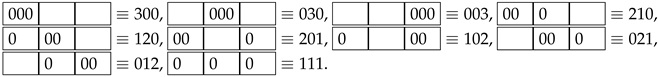
The main parameter of each macrostate is the corresponding number of microstates w. If the number of all microstates of the system is $\mathcal{W}=27$, then the probability of a given state is:

$$p={\displaystyle \frac{w}{\mathcal{W}}}={\displaystyle \frac{w}{27}}.$$

(133)

However, Boltzmann-type entropy for macrostates can be calculated by omitting the Boltzmann constant ($k_B:=1$):

$$S=lnw.$$

(134)

The parameters of all macrostates are presented in Table 1. Based on this table, a matrix of elementary entropy differences can be prepared. Table 2. However, for calculating average values, the partial entropy difference matrix taken with the state probability weight Table 3 is more useful. Therefore, on this basis, the most important Table 4 can be made.

As the last table shows, in the example considered, for as many as 9 out of 10 states, the expected value of the entropy change is positive. Only for the most probable state the entropy increase is negative.

4. Conclusions

Based on a broad review of the issue and thorough analysis, three Propositions for the second law of thermodynamics were formulated. Two of them concern phenomenological thermodynamics and one concerns statistical mechanics. Propositions within thermodynamics are not based on the concept of entropy. Proposition 1 corrects the nonexistence of Perpetuum Mobile Second Kind in the Kelvin-Ostwald statement to the more restrictive nonexistence of Perpetuuum Mobile Third Kind. Proposition 2 reinforces the global principle of no heat flow towards any higher temperature (Clausius First Statement) with a stronger Heat-Temperature Inequality. Proposal 3, within the framework of statistical mechanics, uses the concept of elementary probabilistic entropy, but does not use its time evolution in the form of some Liouville equation (such as the Boltzmann equation). Therefore, this proposal called the Probabilistic Scheme of Second Law is free from Loschmidt’s irreversibility paradox. In practice, this means that Proposition 3 allows for a negative entropy change, but this is unlikely or requires the system to be in a particular state. However, the rule is that the entropy increases, but in the sense of the average value and additionally provided that the system is not in the state with the highest entropy.

An interesting property that qualitatively differentiates propositions in the thermodynamic approach from propositions in the probabilistic approach is the status of evidence. The thermodynamic principles (Proposition 1 and 2) cannot be proven directly, but their equivalence to the principle of non-decreasing entropy can be proven. However, a probabilistic statement (e.g. Proposition 3), as it turns out, is subject to direct proof. However, the discussed property does not entitle us to prefer statistical mechanics over phenomenological thermodynamics (or vice versa), as in the dispute over the superiority of Easter over Christmas Eve. The point is that thermodynamic statements are more physical and categorical, and statistical statements are more mathematical and do not contain an absolute and unconditional version of the second law (because they cannot due to fluctuation and the paradox of irreversibility). Therefore, thermodynamics and statistical mechanics must remain complementary and correspond to each other.

Moreover, the work defines new concepts of non-existent machines Perpetuum Mobile - not only Third Kind. At the same time, on the 200th anniversary of Carnot’s work in 1824, it was pointed out that the Carnot engine is not any Perpetuum Mobile, so it should not be just an imaginary theoretical model, but should be technically feasible (in the sense of a machine working on the Carnot comparative cycle). Moreover, in the context of comparing the Heat-Temperature Inequality with the structure of the construction of real numbers given by Eudoxus of Knidos, it is the Carnot engine that corresponds to rational numbers (defined by equalities, not inequalities) - and therefore realizable quantities. In any case, there is no current working prototype of the Carnot engine, and the two existing patents seem a long way from its implementation. It is wrong to think that heat engines are a relic of the past, because even in nuclear power plants electricity is based on steam turbines.

References

- Smoluchowski, M. Gültigkeitsgrenzen des zweiten Hauptsatzes des Wärmetheorie (Limits of validity of the second law of thermodynamics). Vorträge über die kinetische Theorie der Materie und der Elektrizität (Lectures on the kinetic theory of matter and electricity). In Mathematische Vorlesungen an der Universität Göttingen; B.G. Teubner: Leipzig, Germany, 1914; pp. 87–121.
- Wang, L.-S. A Treatise of Heat and Energy, Mechanical Engineering Series, Springer International Publishing, 2019.
- Clausius, R. Ueber die bewegende Kraft der Wärme und die Gesetze, welche sich daraus für die Wärmelehre selbst ableiten lassen (On the Moving Force of Heat, and the Laws regarding the Nature of Heat itself which are deducible therefrom). Ann. Phys.1850, 79, 368–397, 500–524.
- Clausius, R. On the Moving Force of Heat, and the Laws regarding the Nature of Heat itself which are deducible therefrom. Philos. Mag. 1851, 2, 1–21, 102–119.
- Clausius, R. Ueber verschiedene für die Anwendung bequeme Formen der Hauptgleichungen der mechanischen Wärmetheorie (About various forms of the main equations of the mechanical heat theory that are convenient for application). Ann. Phys. Chem. 1854, 169, 481–506. [Google Scholar] [CrossRef]
- Clausius, R. Ueber eine veränderte Form des zweiten Hauptsatzes der mechanischen Wärmetheorie (On a Modified Form of the Second Fundamental Theorem in the Mechanical Theory of Heat). Ann. Phys. 1854, 93, 481–506. [Google Scholar] [CrossRef]
- Clausius, R. On a Modified Form of the Second Fundamental Theorem in the Mechanical Theory of Heat. Phil. Mag. 1856, 12, 81–98. [Google Scholar] [CrossRef]
- Clausius, R. The Mechanical Theory of Heat, with Its Applications to the Steam Engine and to Physical Properties of Bodies; Archer Hirst, T.A., Ed.; John van Voorst: London, UK, 1867, pp.1-374.
- Clausius, R. The Mechanical Theory of Heat, 1st ed.;Walter, W.R., Translator; Macmillan & Co.: London, UK, 1879; pp. 1–376.
- Zemansky, M.W.; Dittmann, R. Heat and Thermodynamics. In An Intermediate Textbook, 5th ed.; McGraw-Hill Book Company: New York, NY, USA, 1968; pp. 140–167. [Google Scholar]
- Thomson, W. On a universal tendency in nature to the dissipation of mechanical energy. Philos. Mag. 1852, 4, 304–306. [Google Scholar] [CrossRef]
- Thomson, W. On the Dynamical Theory of Heat, with numerical results deduced from Mr Joule’s equivalent of a Thermal Unit, and M. Regnault’s Observations on Steam (Part I–III). Philos. Mag. J. Sci. 1852, 4, 8–21, 105–117, 168–256.
- Zivieri, R. Trend in the Second Law of Thermodynamics, Entropy 2023, 25, 1321.
- Koczan, G.M. Proof of Equivalence of Carnot Principle to II Law of Thermodynamics and Non-Equivalence to Clausius I and Kelvin Principles. Entropy 2022, 24, 392. [Google Scholar] [CrossRef]
- Koczan, G.M. Derivation of Hawking Radiation Part II: Quantum and statistical mechanics of photon states (English translation). Foton 2018, 141, 4–32, (https://foton.if.uj.edu.pl/archiwum/2018/141), translation 2019: (https://www.researchgate.net/publication/330369679).
- Tolman, R. The Principles of Statistical Mechanics, 1st ed.; Oxford University Press: London, Great Britain, 1938; p. 661. [Google Scholar]
- Carnot, S. Réflections Sur La Puissance Motrice Du Feu Et Sur Les Machines propres à Développer Cette Puissance (Reflections On The Motive Power Of Fire And On The Machines Suitable For Developing This Power); Bachelier: Paris, France, 1824. [Google Scholar]
- Carathéodory, C. Untersuchungen über die Grundlagen der Thermodynamik (Investigations into the fundamentals of thermodynamics). Math. Ann. 1909, 67, 355–386. [Google Scholar] [CrossRef]
- Turner, L.A. Simplification of Carathéodory’s Treatment of Thermodynamics. Am. J. Phys. 1960, 28, 781–786. [Google Scholar] [CrossRef]
- Landsberg, P.T. A Deduction of Caratheodory’s Principle from Kelvin’s Principle. Nature 1964, 201, 485–486. [Google Scholar] [CrossRef]
- Dunning-Davies, J. Caratheodory’s Principle and the Kelvin Statement of the Second Law. Connections between the Various Forms of the Second Law of Thermodynamics. Nature 1965, 208, 576–577. [Google Scholar] [CrossRef]
- Radhakrishnamurty, P. A Critique on Caratheodory Principle of the Second Law of Thermodynamics. arXiv arXiv:1103.4359, 2011.
- Boltzmann, L. Weitere Studien über das Wärmegleichgewicht unter Gasmolekülen (Further studies on the heat balance among gas molecules). Wiener Berichte 1872, 66, 275–370. [Google Scholar]
- Boltzmann, L. Further Studies on the Thermal Equilibrium of Gas Molecules. The Kinetic Theory of Gases. Hist. Stud. Phys. Sci. 2003, 1, 262–349. [Google Scholar]
- Boltzmann, L. Bermerkungen über einige Probleme der mechanische Wärmetheorie (Remarks on some problems of the mechanical theory of heat). Wiener Berichte 1877, 75, 62-100; in WA II, paper 39 (1877).
- Boltzmann, L. Über die beziehung dem zweiten Haubtsatze der mechanischen Wärmetheorie und der Wahrscheinlichkeitsrechnung respektive den Sätzen über das Wärmegleichgewicht (About the relationship between the second main theorem of the mechanical heat theory and the probability calculation or the theorems about heat equilibrium). Wiener Berichte 1877, 76, 373-435; in WA II, paper 42.
- Balibrea, F. On Clausius, Boltzmann and Shannon Notions of Entropy. J. Mod. Phys. 2016, 7, 219–227. [Google Scholar] [CrossRef]
- Balibrea, F. On the origin and development of some notions of entropy. Topol. Algebra Appl. 2015, 3.1.
- Planck, M. The theory of heat radiation equation, 1914.
- Boltzmann, L. Über die Mechanische Bedeutung des Zweiten Hauptsatzes der Wärmetheorie (On the mechanical meaning of the second law of heat theory). Wiener Berichte 1866, 53, 195–220. [Google Scholar]
- Jaynes, E. T. (1965). Gibbs vs Boltzmann Entropies. Am. J. Phys. 1965, 33, 391–398. [Google Scholar]
- Sawieliew, I.W. Wykłady z fizyki, tom 1. Mechanika. Fizyka cz ˛asteczkowa (Lectures on physics, vol. 1. Mechanics. Molecular physics), 2nd ed.; Wydawnictwo Naukowe PWN: Warsaw, Poland, 1994; pp. 373–381. [Google Scholar]
- Huang, K. Podstawy Fizyki Statystycznej (Introduction to Statistical Physics), 1st ed.; Wydawnictwo Naukowe PWN: Warsaw, Poland, 2006; pp. 72–76. [Google Scholar]
- Grimus, W. On the 100th anniversary of the Sackur–Tetrode equation. arXiv 2013, arXiv:1112.3748v2. [Google Scholar] [CrossRef]
- Addison, S.R. The Ideal Gas on the Canonical Ensemble. Lecture notes, University of Central Arkansas, April 9, 2003.https://faculty.uca.edu/saddison/Thermal2003/CanonicalIdeal.pdf.
- Lifshitz, E.M. , Pitaevskii, L.P. Kinetyka fizyczna (Physical kinetics); Wydawnictwo Naukowe PWN: Warsaw, Poland, 2013; pp. 4–13. [Google Scholar]
- Dorfman J., R. Wprowadzenie do teorii chaosu w nierównowagowej mechanice statystycznej (An introduction to chaos in nonequilibrium statistical mechanics); Wydawnictwo Naukowe PWN: Warsaw, Poland, 2001; pp. 28–38. [Google Scholar]
- Koczan, G.M. OBRONA "FIZYKI" ARYSTOTELESA: Matematycznie ujednolicona rekonstrukcja niesprzecznej z obserwacją dynamiki Arystotelesa (DEFENSE OF ARISTOTLE’S "PHYSICS": Mathematically unified reconstruction of consistent with observation Aristotle’s dynamics); Wydawnictwo SGGW: Warsaw, Poland, 2023; pp. 115, 152, 153, 173–177.
- Evans, D. J. , Cohen, E. G. Probability of second law violations in shearing steady states. Phys. Rev. Lett. 1993, 71, 2401. [Google Scholar]
- Gallavotti, G. and Cohen, E. G.D. Dynamical Ensembles in Nonequilibrium Statistical Mechanics. Phys. Rev. Lett. 1995, 74, 2694. [Google Scholar]
- Gallavotti, G. and Cohen, E. G.D. Dynamical ensembles in stationary states. J. Stat. Phys. 1995, 80, 931. [Google Scholar]
- Evans, D.J. and Searles, D.J. Equilibrium microstates which generate second law violating steady states, Phys. Rev. E 1994, 50, 1645.
- Evans, D.J. , Searles, D.J. and Mittag, E. Fluctuation theorem for Hamiltonian Systems: Le Chatelier’s principle. Phys. Rev. E 2001, 65, 051105 (2001).
- Wang, G. M. , Sevick, E. M., Mittag, Emil, Searles, Debra J., Evans, Denis J. (2002). Experimental Demonstration of Violations of the Second Law of Thermodynamics for Small Systems and Short Time Scales. Phys. Rev. Lett. 2002, 89, 050601.
- Evans, D.J. The Fluctuation Theorem and its Implications for Materials Processing and Modeling, Handbook of Materials Modeling, pp.2773–2776. S. Yip (ed.) 2005 Springer. Printed in the Netherlands.
- Carberry, D. M. , Reid, J. C., Wang, G. M., Sevick, E. M., Searles, Debra J., Evans, Denis J. Fluctuations and Irreversibility: An Experimental Demonstration of a Second-Law-Like Theorem Using a Colloidal Particle Held in an Optical Trap. Phys. Rev. Lett. 2004, 92, 140601.
- Glen, J. S., Edwards, T. C. Heat engine, refrigeration and heat pump cycles approximating the Carnot cycle and apparatus therefor. United States Patent 1991, US5027602A, (https://patents.google.com/patent/US5027602A/en).
- Zhen Ch. Carnot cycle heat engine. Chinese Patent 2013, CN103437909A, (https://patents.google.com/patent/CN103437909A/en).
- Kordos, M. Jak powstały wszystko opisujące liczby (How did the numbers that describe everything come into being?). Delta 2018, 7, (https://www.deltami.edu.pl/2018/07/jak-powstaly-wszystko-opisujace-liczby/).
- Ramsey, N. Thermodynamics and Statistical Mechanics at Negative Absolute Temperatures. Physical Review. 1956, 103(1), 20–28. [Google Scholar] [CrossRef]
- Braun, S., Ronzheimer, J.P., Schreiber, M., Hodgman, S. S., Rom, T., Bloch, I., Schneider U. Negative Absolute Temperature for Motional Degrees of Freedom. Science 2013, 339 (6115), 52–55, (https://arxiv.org/abs/1211.0545). [CrossRef]
- Wiśniewski, S. Termodynamika techniczna (Technical thermodynamics); Wydawnictwo Naukowo Techniczne WNT: Warsaw, Poland, 2017. [Google Scholar]