
Submitted:
12 November 2024
Posted:
13 November 2024
You are already at the latest version
Abstract
False data injection attack (FDIA) is one of the major threats to power systems, and identifying false data is critical to the stable operation of power systems. However false data that closely resemble normal data hinder the accuracy of existing detection methods, and their performance further declines when exposed to ambient noise. To address these challenges, this paper proposes an attentional convolutional neural network based on distinction enhancement and information fusion (DEIF-ACNN) for FDIA detection. Firstly, by minimizing the loss of reconstruction and discrimination, this paper designed an autoencoder with a discriminator for normal data (NAE), which had the characteristic of producing small loss for normal data. Secondly, the trained NAE is utilized to compute the feature correlation matrix between the original and reconstructed data to enhance the distinction between normal and false data. Finally, to enhance feature extraction and suppress ambient noise interference in detection, DEIF-ACNN incorporates a convolutional block attention module (CBAM) to emphasize key feature channels and highlight crucial regions in the feature matrix. Experimental results show that DEIF-ACNN outperforms other FDIA detection methods on IEEE-9, IEEE-14 and IEEE-118 bus power systems. In addition, the method exhibits the best robustness under different noise environments.
Keywords:
power system
; false data injection attack
; CNN
; autoencoder
; attention mechanism
1. Introduction
The development of information technology for power systems brings a lot of convenience, but also increased the power system is exposed to a variety of cyber-attack risk [1,2,3,4]. Among these risks, false data injection attack (FDIA) is one of the most challenging cyber-attacks in power systems [5]. Figure 1 illustrates the attack process of FDIA, hackers will hijack the measurement data of the power system, and according to the system topology and prior knowledge, tamper with it to make it false data, thereby bypassing the bad data detection mechanism in the system [6,7], leading to wrong decisions [8], and may trigger major consequences such as large-scale power outages [9].
Currently, FIDA detection methods are mainly categorized into model-based and data-driven approaches [10]. Model-based detection methods rely on the physical model and priori knowledge of power systems. Therefore, these methods have low scalability [11]. Data-driven detection methods rely on historical measurement data to enable real-time or near real-time inspection through rapid data processing and analysis [12]. However, with the continuous evolution of attack methods, the false data generated by attackers becomes extremely like normal data in terms of features, which may lead to false alarms or omissions in detection results. In addition, the above detection methods do not fully consider the interference of noise in the actual environment on the measurement data, which further reduces the detection efficiency. To address these challenges, this paper proposes DEIF-ACNN model to identify FDIA.
Firstly, DEIF-ACNN is used to enhance distinction of data by constructing NAE that produces smaller loss for normal data inputs and larger loss for false data inputs. Subsequently, DEIF-ACNN fuses the information from the original data and the enhanced data to generate a feature correlation matrix, thus preserving the original information and adapting it to subsequent detection tasks. Finally, DEIF-ACNN introduces CBAM to compute the attention weight matrix from both channel and spatial perspectives, which enhances the key feature channels and highlights the important regions while suppressing the noise interference, thus improving the efficiency of false data detection. The main contributions of this paper are as follows:
- A data-driven FDIA detection method is proposed to identify false data that bypasses the traditional bad data detection (BDD) mechanism to further improve the security of power system.
- The method is completely data-driven and has excellent scalability without considering the physical model and topology of the power system.
- The proposed method is validated by simulation on IEEE-9, IEEE-14, and IEEE-118 bus systems, considering the interference of measured data in real environments.
The rest of the paper is organized as follows: section 2 describes the relate work on FDIA detection techniques in recent years; section 3 describes the fundamentals of power system state estimation and FDIA attacks; section 4 describes the proposed methodology of this paper in detail; section 5 demonstrates the simulation results and performance evaluations on three IEEE standard test systems; and section 6 concludes the work of this paper.
2. Related Work
The current detection methods can be categorized into model-based and data-driven based detection methods.
2.1. Based on Model Detection Method
At the beginning of the study, Duan J et al. used a weighted least squares method to identify FDIAs in power systems, using state estimation to compare with actual measurements in order to detect deviations[13]; Li B’s team proposed a proactive defense approach (PAMA) to protect the grid configuration information and raw measurement data by encrypting the raw measurement data while protecting the grid configuration information [14]; M. G. Kallitsis et al. proposed an adaptive statistical detection method that uses measurements from trusted nodes to detect other anomalous nodes [15]; In order to improve the real-time performance of FDIA detection, R. Moslemi et al. exploited the near-singular sparsity of the power system to develop an efficient framework for solving the associated maximum likelihood (ML) estimation problem, and then decomposed the FDIA detection method into several local ML estimation problems [16]; With the introduction of dynamic modeling, K. Manandhar et al. proposed a detection method based on the Kalman Filter (KF), their team studied the mathematical model of the power system and used the KF to estimate the variables of the various state processes in the model, and then the estimation results and the system data were fed back to the detector to obtain the detection results [17]. The GoDec algorithm was proposed by B. Li et al. Their approach relies on the low-rank property of the measurement matrix and the sparsity of the attack matrix to reformulate FDIA detection as a matrix separation problem, and the approach was shown to be capable of handling measurement noise and applicable to large-scale attacks [18]; S. Li et al. proposed a generalized likelihood ratio based sequence detector to solve the problems of low robustness of the detector and computational inefficiency by considering the sequential detection of FDIA [19].
2.2. Based on Data-Driven Detection Method
With the advent of machine learning and big data technologies, data-driven approaches have emerged as a promising alternative for FDIA detection. Y. He et al. proposed a deep belief network (DBN) based on restricted Boltzmann machine for detecting damaged data in DC power systems [20]; Foroutan S A et al. proposed a semi-supervised method based on Gaussian Mixture Models, they used Gaussian Mixture Models to learn the features of the positive samples and select the appropriate thresholds on the mixed dataset to evaluate the unlabeled data [21]; Similarly, C. Wang et al. used automatic coding to learn the intrinsic features of normal data and predicted positive anomalies by calculating the reconstruction loss, and their approach effectively overcame the challenge of unbalanced data samples in power systems [22]; Convolutional neural network (CNN) is widely used in pattern recognition image processing, and the ability of CNN to extract sample features has become a very promising algorithm for FDIA detection. Min Lu et al. constructed an FDIA model based on improved CNN, which extracts spatial-temporal features of the data by adding a gate recursion unit (GRU) before the fully connected layer of the CNN to achieve efficient, real-time FDIA detection [23].
3. State Estimation and FDIA
This section will introduce the state estimation and BDD technology of power system, sort out the FDIA execution process and analyze the similarity problem between normal and false data.
3.1. State Estimation
The state estimation of power system can be represented by the relationship between the measurement vector and state vector, which is expressed as follows [8]:
where denotes the measurement data, usually the bus voltage, bus active and reactive power injections, and branch active and reactive power flows of power system [9]; denotes state vector; denotes measurement noise obeying a Gaussian distribution ; denotes the functional dependence between the measurements and the state variables, which is usually determined by the system parameters and topology. A common method for solving state vectors is to use the weighted least squares method, in which the state variable estimates are obtained by minimizing a cost function:
where , is the variance of the measurement error of the i-th meter.
Due to the large amount of computation involved in solving the state estimation through multiple iterations, Eq. (1) is simplified to:
where is an Jacobi matrix related to the system parameters and topology. Similarly, solving for the state variable estimates can be done in the following way:
find the closed-form solution:
3.2. BDD Technology
During the operation of the power system, the Bad Data Detection mechanism is used to determine whether the current system-generated measurements contain false data. The basic principle of this mechanism is to substitute the state variable estimate into the residual calculation, a process that can be expressed as follows:
where represents the difference between the actual measured value and the estimated value. In the ideal case, should be close to zero. However, due to measurement errors and potentially bad data, the residual may be larger than a certain threshold. Thus, potential bad data can be identified by residual analysis as shown in the following equation:
where is a threshold set in advance. At this point it can be determined that the system is experiencing bad data.
3.3. False Data Injection Attack
FDIA will inject attack vectors into the measurement data without changing the :
where denotes the measurement vector after the attack. At this point, the system state variable estimate can be expressed as:
at this point the residual can be computed as:
If , it is guaranteed not to change the value of to inject the attack vector into the measurement data. Note that the injection vector can also be obtained without explicitly asking for . In [9], it was shown that the relation can be transformed into an equivalent form without explicitly using , and from this is generated. Since the FDIA constructed through the above is less than as the residual generated in the normal case, then false data can perfectly bypass the BDD and pose a threat to the stable operation of the power system.
3.4. Problem Analysis
The main reason why the false data behaves very similar to the normal data is that the attacker utilizes an in-depth understanding of the power system model. The attacker has access to the parameters and topology of the system and uses the Jacobi matrix to design an attack vector that makes the injected false data behave very similarly to the normal data in terms of features. To quantify this similarity, this paper uses kernel density estimation to estimate the distribution of normal and false data. The kernel density estimation formula is as follows:
where is the estimated probability density function, is the kernel function, is the bandwidth parameter, which controls smoothing, and is the sample point.
The feature distribution of normal data is usually more centralized, showing typical measurements of the system in steady state operation, such as bus voltages, branch active and reactive power flows. False data are injected into the system via attack vectors, which are designed to be highly overlapped with the normal data in terms of features by using the Jacobi matrix to ensure that they satisfy . The false data successfully bypasses the BDD mechanism by modifying the measurement data without changing the residuals . In the probability density distribution plots of normal data and false data shown in Figure 2, the distribution curves of false data are highly overlapped with the normal data curves, and the feature overlap rate reaches 96.27%. This means that the false data is very similar to the normal data in the feature space, causing the existing detection methods to be difficult to distinguish.
Therefore, the detection ability of false data must be improved by enhancing the differentiation between the two.
4. Proposed Detection Method
This section describes the proposed Attentional Convolutional Neural Network based on Distinction Enhancement and Information Fusion (DEIF-ACNN) for detection of FDIA bypassing BDD. Figure 3 illustrates the proposed detection method. DEIF-ACNN consists of two parts, the first part is to compute the feature correlation matrix after distinction enhancement using NAE; the second part is the detection module based on attentional convolutional neural network to extract important features and suppress noise interference.
4.1. Distinction Enhancement and Information Fusion
In the proposed DEIF-ACNN method, NAE is constructed to enhance the distinction between the normal and false data, and its specific structure is shown in Figure 4.
When training NAE, only the normal data is taken as input and reconstructed features are computed by NAE, the process can be described as:
where denotes the m-dimensional normal data features; denotes the data encoding computation; denotes the data decoding computation; and denote the parameters of the encoder and decoder, respectively, and denotes the m-dimensional reconstructed feature vector. The mean square error is chosen as the loss function for the reconstruction error and the calculation process is shown in Equation (14):
where denotes the number of samples per small batch.
To better ensure that the reconstructed data features belong to the type of normal data, NAE introduces a discriminator. This discriminator is trained using the normal data and the loss is computed using a binary cross-entropy loss function in the following procedure:
where denotes the internal parameters of the discriminator; denotes the discriminator and denotes the prediction result of the discriminator. By minimizing the loss, the internal parameters of the discriminator are updated until the loss converges. At this point, the reconstructed data features are used as inputs to the discriminator to obtain the prediction results, which are calculated as follows:
where denotes the prediction result of the discriminator on the reconstructed data. Then the discrimination loss of the discriminator for the reconstructed features is calculated:
Combining equation (13) and (17) yields the final loss value for NAE:
The NAE parameters and are updated by minimizing . In this way, the NAE is equipped with the characteristic of incurring smaller losses for normal data and larger losses for false data.
Next, DEIF-ACNN takes the hybrid data as input and computes the reconstructed data features through the trained NAE. Due to the characteristic of NAE, the following inequality will be satisfied:
where denotes false data. According to Equation (19), the distinction enhanced feature vectors can be computed by equation (20):
where denotes the corresponding positional subtraction of the feature vector and E denotes the enhanced data feature. Figure 5 shows the distribution of normal data and false data after distinction enhancement. Comparing with Figure 2, it can be clearly seen that the distribution overlap of the two types of data is significantly reduced, and the overlap rate is reduced to 87.03%.
To ensure that the original data feature information is not lost during enhancing the distinction process and to satisfy the input requirements of the subsequent detection modules. DEIF-ACNN generates feature correlation matrix by feature vector correlation after distinction enhancement. The process is described as:
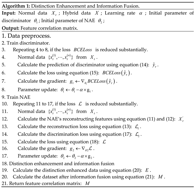
Therefore, the flow of the DEIF-ACNN model in the distinction enhancement and information fusion phase is shown in Algorithm 1.
4.2. Attention Convolutional Neural Network
After processing in Section 4.1, each sample in the original data has been transformed into a feature correlation matrix. To improve the accuracy of FDIA detection, this method uses CNN with a built-in attention mechanism module for better extraction of the data features of the feature correlation matrix. The structure is shown in the detection module of Figure 3. The ACNN consists of multiple feature extraction layers, each of which includes a convolutional layer, a CBAM module, and a pooling layer.
In ACNN, the convolutional layer of each feature extraction layer consists of multiple learnable convolutional kernels. The key operations of the convolutional layer include local correlation and window sliding. Local correlation means that each convolution kernel is considered as a window filter, and during neural network training, the convolution kernels are convolved with the input data according to a customized size. Then, by controlling the step size, the sliding distance of the window filter is determined so that features are extracted in each localized region. The convolution process is essentially the multiplication of two matrices, and after convolution, the dimensions of the input data are reduced.
In the convolutional layer, in addition to the convolution operation, there are two key parameters: the activation function and the learnable bias vector. The role of the bias vector is to perform a linear addition of the convolved data, i.e., the convolution result is added to the bias vector, as shown in equation (22). The activation function is used to enhance the nonlinear capability of the network by activating the data to remove useless information.
where is the feature mapping of the input feature matrix after the convolution operation of the i-th feature extraction layer; is the j-th convolution kernel of the i-th convolution layer; denotes the convolution operation; is the j-th bias vector of the i-th convolution layer; denotes the activation function.
To extract the locally important information more effectively and suppress the noise interference, ACNN introduces the CBAM module based on the attention mechanism after the convolutional layer, and its specific structure is shown in Figure 6. CBAM is a lightweight module with low memory requirements and computational cost, conditions that are extremely favorable for power system applications. CBAM consists of two sub-modules: channel attention module (CAM) and spatial attention module (SAM), which help to emphasize relevant information from different perspectives. CAM highlights channels associated with change while suppressing irrelevant channels; SAM amplifies the difference between changed and unchanged feature elements in the spatial dimension. In this way, CBAM more accurately identifies extremely important regions of the feature matrix.
CBAM takes the output of the previous convolutional layer as input, computes the attention weight matrix in channel and spatial dimensions, and finally multiplies the input feature matrix with the attention weight matrix to obtain a new feature matrix. The process is described as follows:
indicates that the CAM sub-module computes the channel attention weight matrix; indicates that the SAM sub-module computes the spatial attention weight matrix; , and denote the input feature matrix, the feature matrix after the channel attention, and the final output feature matrix, respectively.
In computing the channel attention weights, the CAM submodule takes the original feature matrix as input and applies maximum pooling and average pooling, respectively; Subsequently, the pooling results are processed through a multilayer perceptron (MLP) based on an encoder-decoder architecture; Finally, the channel attention feature matrix is generated by Sigmoid activation function. The process is shown in Equation (25):
where and denote the weights of the first and second hidden layers of the MLP, respectively; denotes the Sigmoid activation function. The new feature matrix is obtained by multiplying the channel attention weight matrix with the input feature matrix.
In computing the spatial attention weight matrix, the SAM sub-module first performs average pooling and maximum pooling operations on the feature matrix along the channel axis, respectively; then, these two pooled feature maps are spliced on the channel axis to form a combined feature matrix; subsequently, a 7*7 convolution operation is performed on the combined feature matrix; and finally, the spatial attention weight matrix is generated by the Sigmoid activation function. The process is shown in equation (25):
where denotes a convolution operation using a 7*7 convolution kernel. The spatial attention weight matrix is multiplied with the output of the CAM sub-module to finally obtain the output of the CBAM.
The CBAM module further captures important information about the output results of the convolutional layer and suppresses the interference of noise in the feature matrix. To reduce the subsequent computational complexity, ACNN adds a pooling layer after the CBAM module, aiming at compressing the data and the number of parameters and reducing the risk of overfitting, while preserving the most important features in the data. The pooling layer operates as follows:
- Feature invariance: pooling operation removes unimportant information in data features, while the retained information is scale invariance and still representative of the data features before pooling.
- Feature dimensionality reduction: the pooling layer reduces the data dimensionality by removing redundant information and extracting only the most important features, thus reducing the amount of computation and preventing overfitting to a certain extent.
The last layer of the ACNN is the linear layer, whose main function is to compute the final prediction probability from the features extracted from the feature extraction layer through the fully connected network, whose structure is shown in Figure 7. First, the feature matrices are converted to feature vectors by a flatten layer, since the input to the linear layer requires one-dimensional feature vectors rather than matrices. Next, the feature vectors are processed through a fully connected network to generate predictions. Finally, the model is optimized by calculating the loss between the ACNN predictions and the true labels. The loss is calculated using the cross-entropy loss function as follows:
where denotes the amount of data in each small batch; denotes the true label of the i-th sample; denotes the probability that the i-th sample is predicted to have a positive label. The internal parameters of the ACNN are adjusted to optimize the model performance by minimizing the loss values calculated by equation (26).
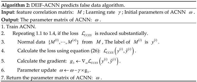
Therefore, the process of training DEIF-ACNN model to predict false data is shown in Algorithm 2.
5. Experiments
In this section, the effectiveness of the proposed method on the IEEE-9, IEEE-14, and IEEE-118 bus power system standard test systems is analyzed in detail and the performance of the method in a noisy environment is explored.
5.1. Dataset Setup
The datasets used in this experiment were collected from IEEE-9, IEEE-14 and IEEE-118 standard test case simulations. These test cases are from PYPOWER, a derivative of MATPOWER [24].
5.1.1. Simulation Case Description
The IEEE-9 bus is a test case consisting of 9 buses, 3 generators and 9 branches; the IEEE-14 bus consists of 14 buses, 5 generators and 20 branches; and the IEEE-118 bus consists of 118 buses, 54 generators and 186 branches. The topologies of IEEE-9 and IEEE-14 are shown in Figure 8. Due to the huge IEEE-118 system, the topology diagram of IEEE-118 bus is omitted in this paper, and the details can be seen in [25]. The main system parameters for the test case are shown in Table 1. where the PF and QF of the branch are only included in the power flow output and are ignored when used as inputs to the power flow.
5.1.2. Data Generation
Since PYPOWER has only one test case for IEEE-9, IEEE-14 and IEEE-118 bus, the generated data is insufficient to support the whole experiment. Therefore, to be able to obtain more data, each bus system will be assigned about 100k load data [26], each of which includes both active and reactive loads. The process of generating measurement data is as follows:
Step 1: Modify the active demand and reactive demand of the simulated system using this load data. The modifications are as follows:
where denotes active load and denotes reactive load. Each modification becomes a new test case. The new test case is input to the AC-PF of PYPOWER for Power flow calculation, and measurement data is taken from the results of the calculation. Among the measured data are the bus active power injection (), the bus reactive power injection (), the active power injection at the branch “from” end () and the reactive power injection at the branch “from” end (). The calculation process of the measured data is as follows:
The number of measurements of the measured data in the three test cases is shown in Table 2.
Step 2: a random number from 0 to 1 is generated to determine whether the current measurement data is needed for a false data injection attack by using Equation (8). The conditions are as follows:
Step 3: by using Equation (2) to (7), determine whether the measurement data obtained by the current system satisfies the residual analysis. If the residual analysis is satisfied, add it to the dataset collection; if not, return to Step 1.
Repeat step 1 to step 3 until all load data is used up.
5.1.3. Data Preprocessing
To maximize the performance of all models used in the experiment, the collected dataset will be preprocessed.
- Balancing Process. From the generated dataset, 15k normal data and 15k false data were randomly selected to form the sample balanced dataset, details are given in Table 3.
- Normalization Process. The features of the dataset are deflated to between [0,1]. The deflation process is as follows:
where min and max are the minimum and maximum values of the sample data, respectively.

Table 3.
Specifics of the datasets.
| Bus name | Bus-9 | Bus-14 | Bus-118 |
|---|---|---|---|
| Normal data | 15000 | 15000 | 15000 |
| False data | 15000 | 15000 | 15000 |
| Number of features | 36 | 68 | 608 |
| Total | 30000 | 30000 | 30000 |
- 3.
- Dataset splitting. Throughout the experiments, each dataset was divided into 60% training set, 20% validation set and 20% test set.
5.2. Evaluation Metrics
Accuracy, precision, recall, F1-Score and cross-entropy loss are considered as evaluation metrics to measure the performance of classification models, and they are defined below:
where TP is True Positive, TN is True Negative, FP is False Positive and FN is False Negative. F1-Score can comprehensively evaluate the performance of the model, and therefore is the evaluation metric that is the focus of comparison in this paper; The cross-entropy loss reflects the convergence of the model during the training process.
5.3. FDIA Detection Performance
To assess the detection efficiency and reliability of the method in this paper, a comparative experiment was conducted with several baseline models.
5.3.1. Ideal Environment
In the experimental evaluation, this paper first conducts a comparison experiment in an ideal environment (no noise condition). The experimental results are shown in Table 4, where the No-CBAM is the ablation model of the proposed method in this paper, specifically the removal of the CBAM module in the ACNN.
In the IEEE-9 bus system, DEIF-ACNN has an accuracy of 99.22%, precision of 99.97%, recall of 98.48%, and F1-Score of 99.22%. Compared with other optimal models (e.g., DT), the F1-Score improves by 0.42%. This smaller boost reflects the fact that DT already performs quite well when dealing with a system of this size. However, the distinction enhancement and information fusion strategies of DEIF-ACNN enable it to better mine the subtle differences in the data, combined with the optimized extraction of features by the CBAM module, it further improves the comprehensive performance of the model. In contrast, weaker models such as AE perform significantly worse in this system, with an F1-Score of only 88.20%. This is mainly since AE is not able to extract the important features as DEIF-ACNN does when dealing with complex data features, thus the performance gap between the two is significant.
In the IEEE-14 bus system, DEIF-ACNN has an accuracy of 99.83%, a precision of 100%, a recall of 99.67%, and an F1-Score of 99.83%. Compared with other better performing models (e.g., CNN), the F1-Score is only improved by 0.43%. CNN has already demonstrated a fairly good performance in this system due to its powerful feature extraction capabilities. However, DEIF-ACNN further enhances the capture of key features by incorporating the CBAM of the attention mechanism, thus achieving a small but significant performance improvement over the already high level. In contrast, the F1-Score of the AE is only 84.36%, which further indicates that the feature extraction ability of the AE is much less than that of DEIF-ACNN when dealing with more complex system structures.
In the IEEE-118 bus system, DEIF-ACNN achieves 100% accuracy, precision, recall and F1-Score, which is an excellent performance. The accuracy is improved by 41.2% compared to the worst KNN. This is since KNN classifies the data by calculating the Euclidean distance, which makes it difficult to perform well with high dimensional data. However, some other models (e.g., MLP, CNN, DBN, and No-CBAM) also achieve the same high scores. This situation is difficult to compare further. Therefore, the advantage of the model is evaluated by observing the change of cross-entropy loss during the training process. As shown in Figure 9, DEIF-ACNN converges faster during the training process, indicating that it has significant advantages in learning efficiency and training stability. This also implies that DEIF-ACNN may have stronger generalization ability and higher reliability in more complex practical application scenarios.
In summary, although the improvement of DEIF-ACNN is limited when compared with better-performing models, its stable performance and superiority in complex systems still reflect its strong detection ability. Compared with the poorer performing models, DEIF-ACNN significantly improves the detection efficiency, mainly due to its effective combination of distinction enhancement, information fusion, and attention mechanism. The overall results of the comparison experiments are shown in Figure 10.
5.3.2. Noise Environment
In practical application environments, the interference of noise for measurement data such as electromagnetic waves can significantly affect the detection efficiency of the detection model. Therefore, this section evaluates the detection efficiency under different noise levels. In this experiment, Gaussian noise is used to simulate the interference to the measurement data in the real environment. The process of adding noise is as follows:
where denotes the m-dimensional original data, denotes m-dimensional noise vector obeying a Gaussian noise , indicates data after adding noise. Different values of indicate the level of noise, the higher the value of , the higher the noise level and the stronger the interference. The interference of different levels of noise on the detection results is modeled by varying the magnitude of , the values of are specifically shown in Table 5.
In the process of extracting important features, DEIF-ACNN employed CBAM to mitigate noise interference in the detection process. The heatmaps of extracted features were plotted on the three datasets for original data, noisy data, and data with noise suppressed, respectively. For visualization purposes, 60 samples were randomly selected as observations in the test set and the extracted features were nonlinearly mapped to a low-dimensional space (32 dimensions) by an autoencoder. The corresponding heatmaps are shown in Figure 11, Figure 12, and Figure 13. The horizontal axis of each heatmap represents the individual feature of the samples, and the vertical axis represents each sample. The color scale from blue to red indicates the magnitude of the eigenvalue. Comparing (a) and (b) of Figure 11, 12, and 13, the heatmaps drawn by features extracted from the noisy data have changed significantly, this situation may lead to a decrease in accuracy. As shown in Figure 14. By utilizing CBAM to suppress the interference of noise, the overall pattern of the heatmap after the noise suppressed is close to the original data, as can be seen in (c) of Figures 11, 12, and 13. This is because CBAM adaptively adjusts the contribution of features by calculating attention weights. Thus, the effect of noise on the detection performance of DEIF-ACNN is reduced. Overall, the noise suppression strategy of DEIF-ACNN is effective and greatly restores the features of the noisy data.
To further illustrate the effectiveness of DEIF-ACNN in suppressing noise, the classification accuracies of DEIF-ACNN were compared with several other detection models under different noise conditions. As shown in Figure 14(a), the proposed method outperforms the other models in terms of accuracy under different noise conditions. With the increasing noise level, the accuracy of DEIF-ACNN remains around 80%. However, for DBN, the accuracy decreases to about 50%. This suggests that these models have difficulty dealing with complex feature relationships in noisy environments. Observing Figure 14(b), although the accuracy of AE improves by 5% within the noise level from 0 to 0.2, the accuracy of AE decreases to about 75% as the noise level continues to increase. This is because moderate noise acts as a regularization factor and enhances the generalization ability of the model. The results on the IEEE-14 bus dataset show that DEIF-ACNN still has the strongest resistance to noise interference. On the IEEE-118 bus dataset, as shown in Figure. 14(c), as the noise level increases, the accuracy decreases from 60% to 50% since the KNN does not have the feature extraction capability. MLP has a weaker feature extraction capability, and the accuracy of MLP decreases from 100% to 50%. Similarly, the same situation as for the IEEE-14 bus occurred at a noise level of around 1 on this dataset. This further indicates that moderate noise enhances the generalization ability of the model.
Overall, the proposed method consistently maintains high classification accuracy across all noise levels, particularly in high-noise environments, where it demonstrates stronger robustness and anti-interference capabilities. The DEIF-ACNN is compared with No-ACNN on all datasets. The comparison results further demonstrate the effectiveness of DEIF-ACNN for combating noise interference. In comparing No-CBAM with other methods, it is illustrated that DEIF-ACNN still enhances the distinction between normal and false data in noisy environments. All experimental results demonstrate the ability of DEIF-ACNN to improve the distinction between normal and false data, as well as verifying the ability of DEIF-ACNN in resisting noise interference.
6. Conclusion
This paper proposes an FDIA detection method based on DEIF-ACNN. Firstly, DEIF-ACNN constructs a NAE to enhance distinction of the data, and then converts the original data and the enhanced data into a feature correlation matrix through information fusion. Meanwhile, to better extract the data features and suppress the noise interference in the data, DEIF-ACNN also incorporates the CBAM module based on the attention mechanism. The performance of the model is evaluated in ideal and noisy environments on IEEE-9, IEEE-14 and IEEE-118 bus systems, respectively. In the ideal environment, the experimental results show that the effectiveness of DEIF-ACNN in detecting FDIA; in the noisy environment, by analyzing the heatmap of extracted features, it is shown that DEIF-ACNN successfully suppresses the noise and improves the detection accuracy. It also proves that DEIF-ACNN is a noise suppression strategy. Therefore, DEIF-ACNN provides a new idea for FDIA detection methods in power systems. However, the current method proposed in this paper has some limitations and can only solve simpler binary classification problems. In future work, we will apply this research to more complex system environments.
7. Patents
This work was supported by the Chinese Government Guidance Fund on Local Science and Technology Development of Sichuan Province (24ZYRGZN0018).
References
- Dehghanpour, K.; Wang, Z.; Wang, J.; Yuan, Y.; Bu, F. A Survey on State Estimation Techniques and Challenges in Smart Distribution Systems. in IEEE Transactions on Smart Grid, vol. 10, no. 2, pp. 2312-2322, March 2019. [CrossRef]
- Fang, X.; Misra, S.; Xue, G.; Yang, D. Smart Grid — The New and Improved Power Grid: A Survey,” in IEEE Communications Surveys & Tutorials, vol. 14, no. 4, pp. 944-980, Fourth Quarter 2012. [CrossRef]
- Spanò, E.; Niccolini, L.; Pascoli, S.D.; Iannacconeluca, G. Last-Meter Smart Grid Embedded in an Internet-of-Things Platform,” in IEEE Transactions on Smart Grid, vol. 6, no. 1, pp. 468-476, Jan. 2015. [CrossRef]
- Sridhar, S.; Hahn, A.; Govindarasu, M. Cyber–Physical System Security for the Electric Power Grid,” in Proceedings of the IEEE, vol. 100, no. 1, pp. 210-224, Jan. 2012. [CrossRef]
- Deng, R.; Xiao, G.; Lu, R.; Liang, H.; Vasilakos, A.V. False Data Injection on State Estimation in Power Systems—Attacks, Impacts, and Defense: A Survey,” in IEEE Transactions on Industrial Informatics, vol. 13, no. 2, pp. 411-423, April 2017. [CrossRef]
- Li, F.; et al. Smart Transmission Grid: Vision and Framework,” in IEEE Transactions on Smart Grid, vol. 1, no. 2, pp. 168-177, Sept. 2010. [CrossRef]
- Yu, Z.-H.; Chin, W.-L. Blind False Data Injection Attack Using PCA Approximation Method in Smart Grid,” in IEEE Transactions on Smart Grid, vol. 6, no. 3, pp. 1219-1226, May 2015. [CrossRef]
- Liang, G.; Zhao, J.; Luo, F.; Weller, S.R.; Dong, Z.Y. A Review of False Data Injection Attacks Against Modern Power Systems,” in IEEE Transactions on Smart Grid, vol. 8, no. 4, pp. 1630-1638, July 2017. [CrossRef]
- Liu, Y.; Ning, P.; Reiter, M.K. 2011. False data injection attacks against state estimation in electric power grids. ACM Trans. Inf. Syst. Secur. 14, 1, Article 13 (May 2011), 33 pages. [CrossRef]
- Li, X.; Hu, L.; Lu, Z. Detection of false data injection attack in power grid based on spatial-temporal transformer network[J]. Expert Systems with Applications, 2024, 238: 121706.
- Li, Y.; Wang, Y. Developing graphical detection techniques for maintaining state estimation integrity against false data injection attack in integrated electric cyber-physical system[J]. Journal of systems architecture, 2020, 105: 101705.
- Musleh, A.S.; Chen, G.; Dong, Z.Y. A Survey on the Detection Algorithms for False Data Injection Attacks in Smart Grids,” in IEEE Transactions on Smart Grid, vol. 11, no. 3, pp. 2218-2234, May 2020. [CrossRef]
- Duan, J.; Zeng, W.; Chow, M.-Y. Resilient Distributed DC Optimal Power Flow Against Data Integrity Attack,” in IEEE Transactions on Smart Grid, vol. 9, no. 4, pp. 3543-3552, July 2018. [CrossRef]
- Li, B.; Lu, R.; Xiao, G.; Su, Z.; Ghorbani, A. PAMA: A Proactive Approach to Mitigate False Data Injection Attacks in Smart Grids,” 2018 IEEE Global Communications Conference (GLOBECOM), Abu Dhabi, United Arab Emirates, 2018, pp. 1-6. [CrossRef]
- Kallitsis, M.G.; Bhattacharya, S.; Stoev, S.; Michailidis, G. Adaptive statistical detection of false data injection attacks in smart grids,” 2016 IEEE Global Conference on Signal and Information Processing (GlobalSIP), Washington, DC, USA, 2016, pp. 826-830. [CrossRef]
- Moslemi, R.; Mesbahi, A.; Velni, J.M. A Fast, Decentralized Covariance Selection-Based Approach to Detect Cyber Attacks in Smart Grids,” in IEEE Transactions on Smart Grid, vol. 9, no. 5, pp. 4930-4941, Sept. 2018. [CrossRef]
- Manandhar, K.; Cao, X.; Hu, F.; Liu, Y. Detection of Faults and Attacks Including False Data Injection Attack in Smart Grid Using Kalman Filter,” in IEEE Transactions on Control of Network Systems, vol. 1, no. 4, pp. 370-379, Dec. 2014. [CrossRef]
- Li, B.; Ding, T.; Huang, C.; Zhao, J.; Yang, Y.; Chen, Y. Detecting False Data Injection Attacks Against Power System State Estimation With Fast Go-Decomposition Approach,” in IEEE Transactions on Industrial Informatics, vol. 15, no. 5, pp. 2892-2904, May 2019. [CrossRef]
- Li, S.; Yılmaz, Y.; Wang, X. Quickest Detection of False Data Injection Attack in Wide-Area Smart Grids,” in IEEE Transactions on Smart Grid, vol. 6, no. 6, pp. 2725-2735, Nov. 2015. [CrossRef]
- He, Y.; Mendis, G.J.; Wei, J. Real-Time Detection of False Data Injection Attacks in Smart Grid: A Deep Learning-Based Intelligent Mechanism,” in IEEE Transactions on Smart Grid, vol. 8, no. 5, pp. 2505-2516, Sept. 2017. [CrossRef]
- Foroutan, S.A.; Salmasi, F.R. (2017), Detection of false data injection attacks against state estimation in smart grids based on a mixture Gaussian distribution learning method. IET Cyber-Physical Systems: Theory & Applications, 2: 161-171. [CrossRef]
- Wang, C.; Tindemans, S.; Pan, K.; Palensky, P. Detection of False Data Injection Attacks Using the Autoencoder Approach,” 2020 International Conference on Probabilistic Methods Applied to Power Systems (PMAPS), Liege, Belgium, 2020, pp. 1-6. [CrossRef]
- Lu, M.; Wang, L.; Cao, Z. , et al. False data injection attacks detection on power systems with convolutional neural network[C]//Journal of Physics: Conference Series. IOP Publishing, 2020, 1633(1): 012134.
- Zimmerman, R.D.; Murillo-Sanchez, C.E.; Thomas, R.J. MATPOWER: Steady-State Operations, Planning and Analysis Tools for Power Systems Research and Education,” Power Systems, IEEE Transactions on, vol. 26, no. 1, pp. 12–19, Feb. 2011.
- Information Trust Institute Grainger College of Engineering (2024). IEEE 118-Bus System. https://icseg.iti.illinois.edu/ieee-118-bus-system/.
- Trindade, A. (2015). ElectricityLoadDiagrams20112014 [Dataset]. UCI Machine Learning Repository. [CrossRef]
Figure 1.
The FDIA of power system.
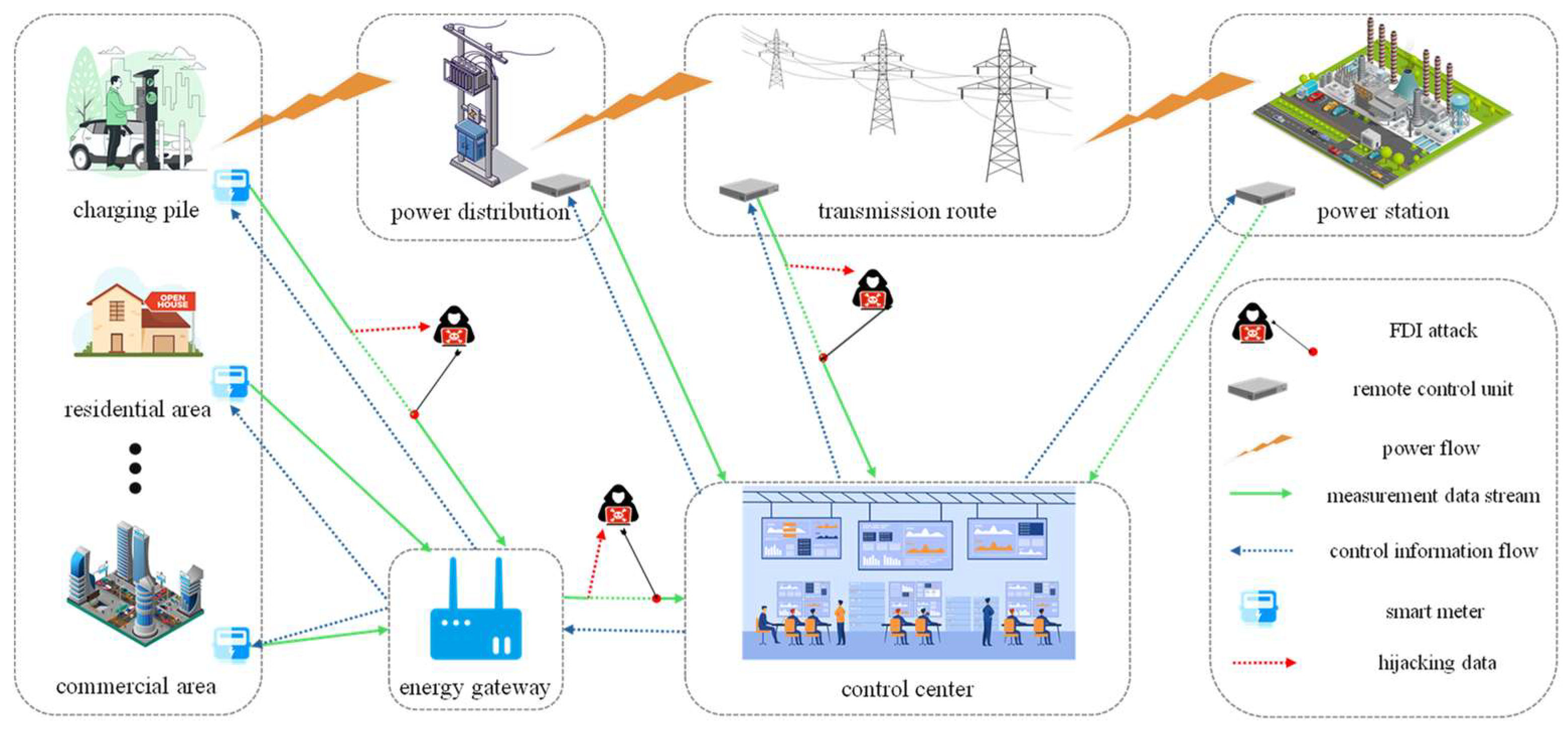
Figure 2.
The distribution of normal and false data.
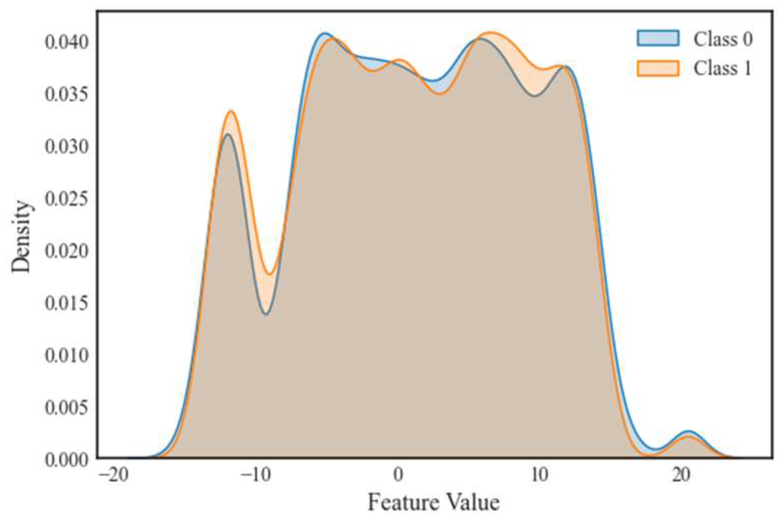
Figure 3.
The structure of the DEIF-ACNN model.
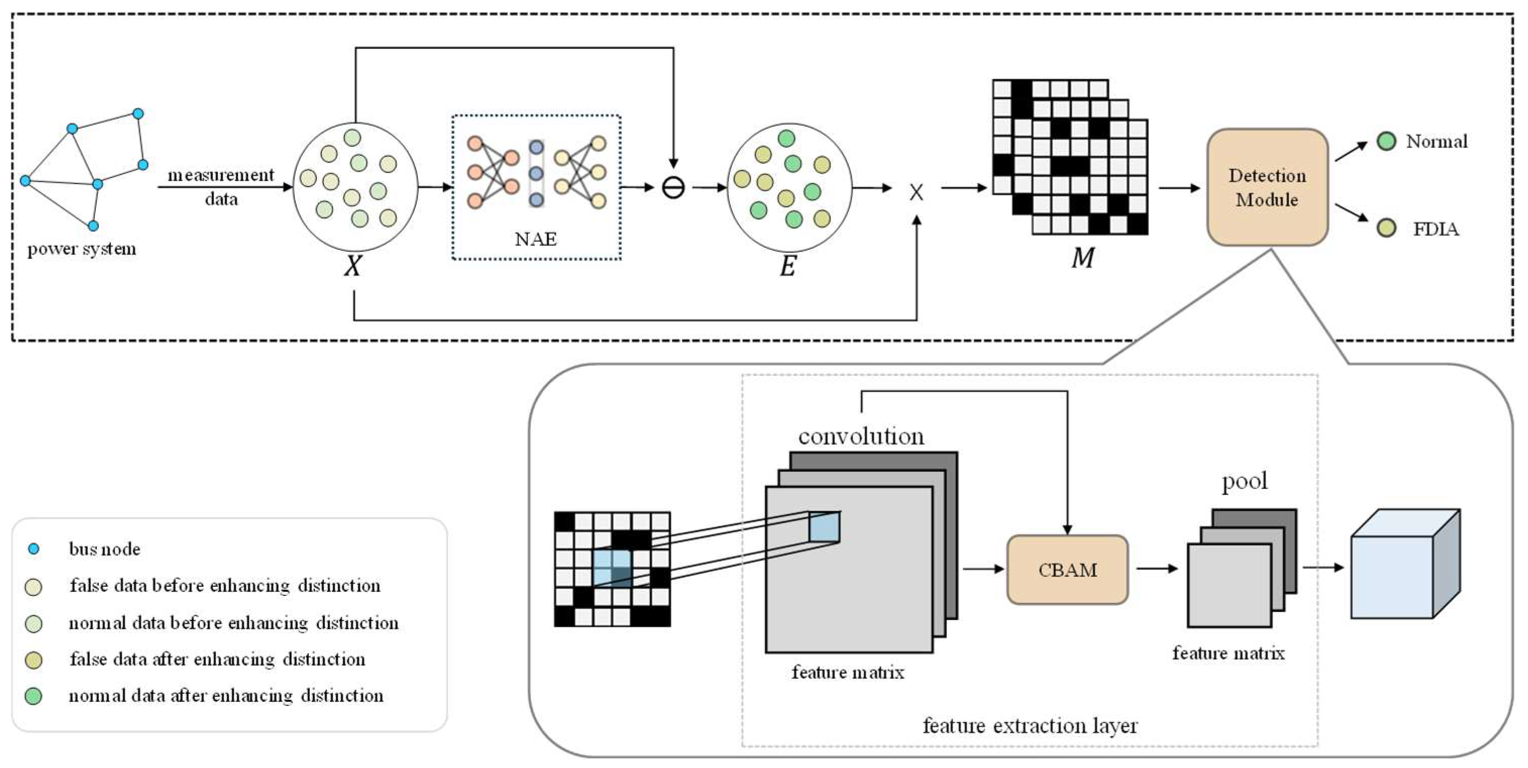
Figure 4.
The structure of the NAE.
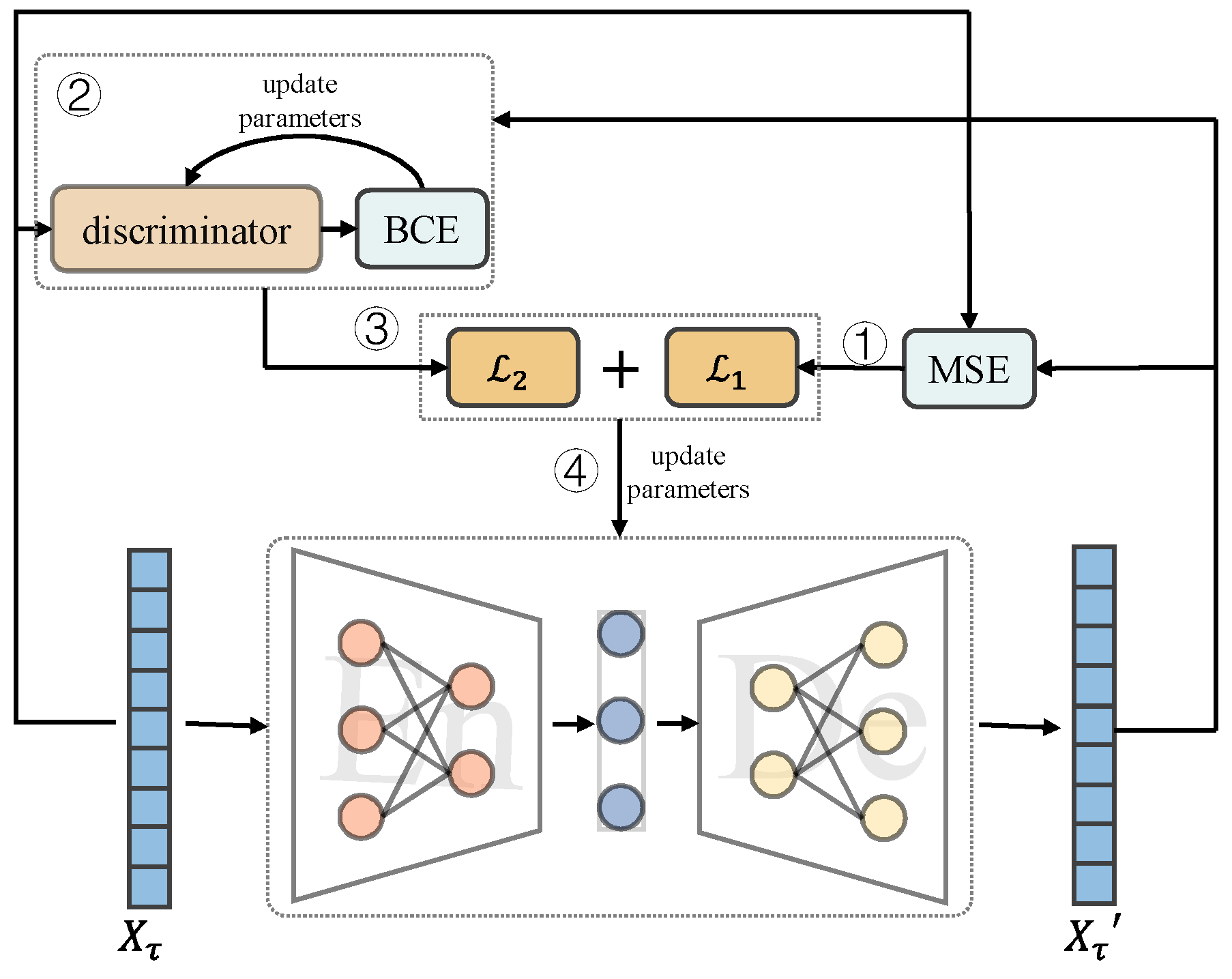
Figure 5.
the distribution of normal and false data after distinction enhanced.
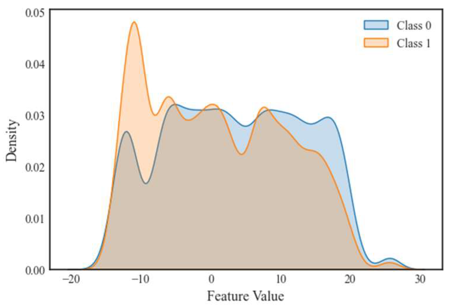
Figure 6.
The internal structure of CBAM module.
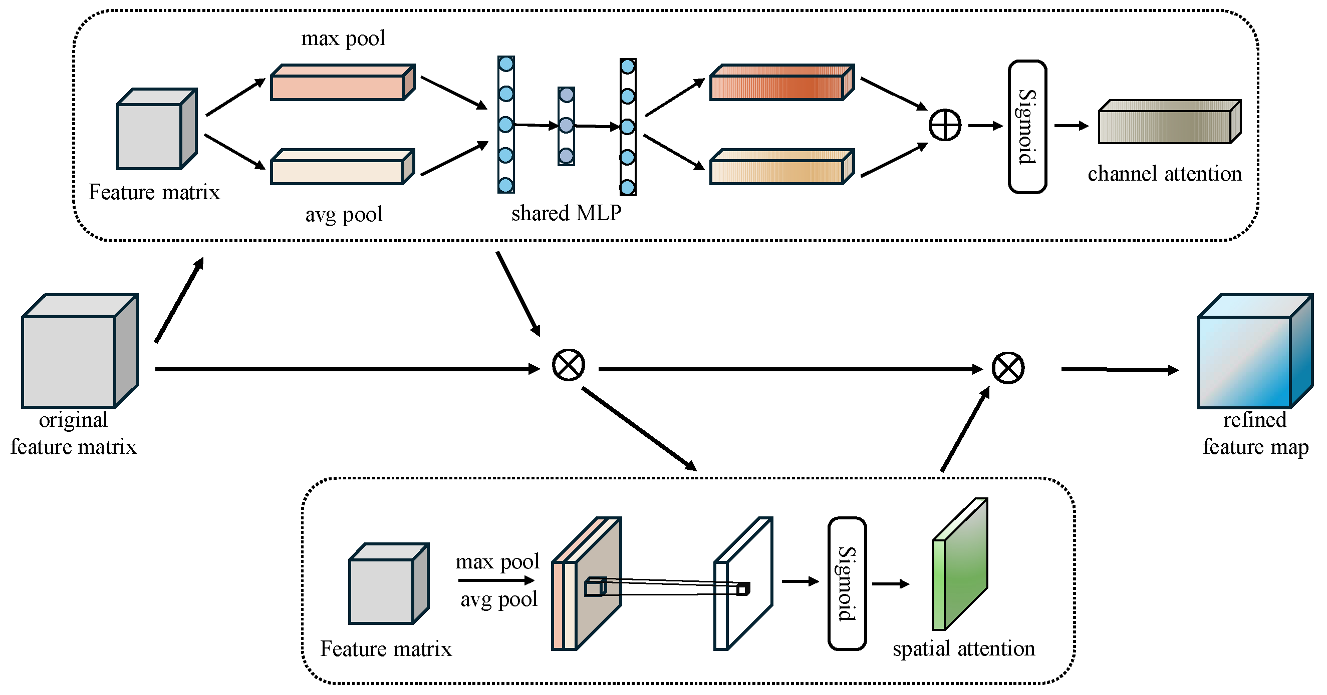
Figure 7.
The fully connected linear layers.
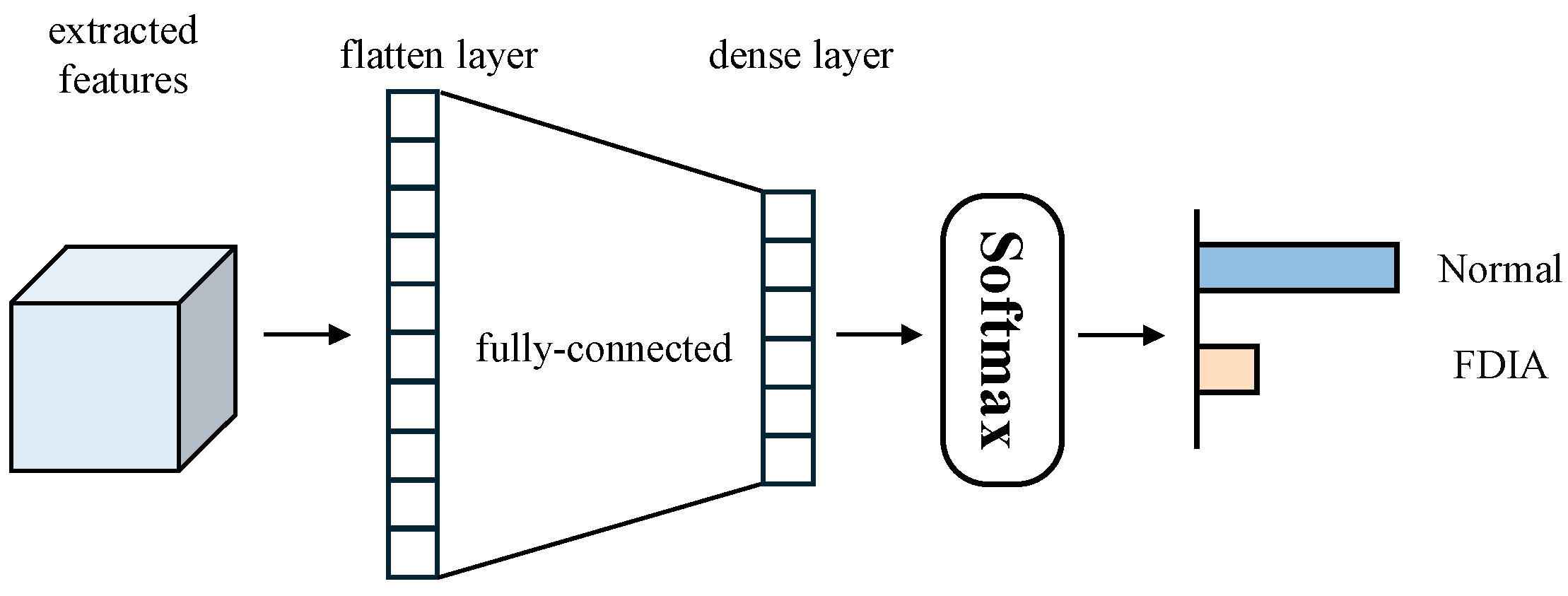
Figure 8.
The topology structure.
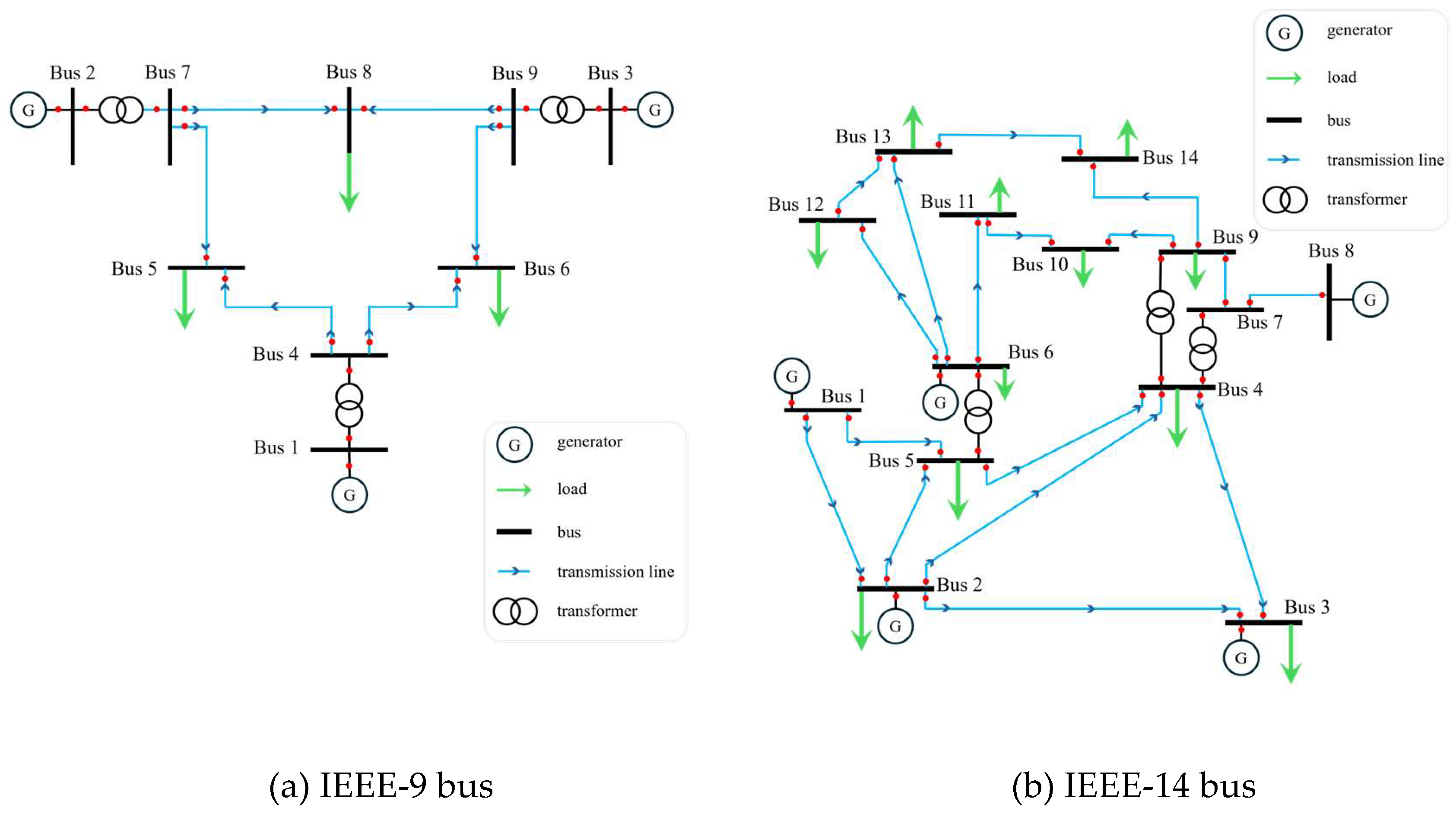
Figure 9.
Changes in accuracy and loss of training on IEEE bus-118.
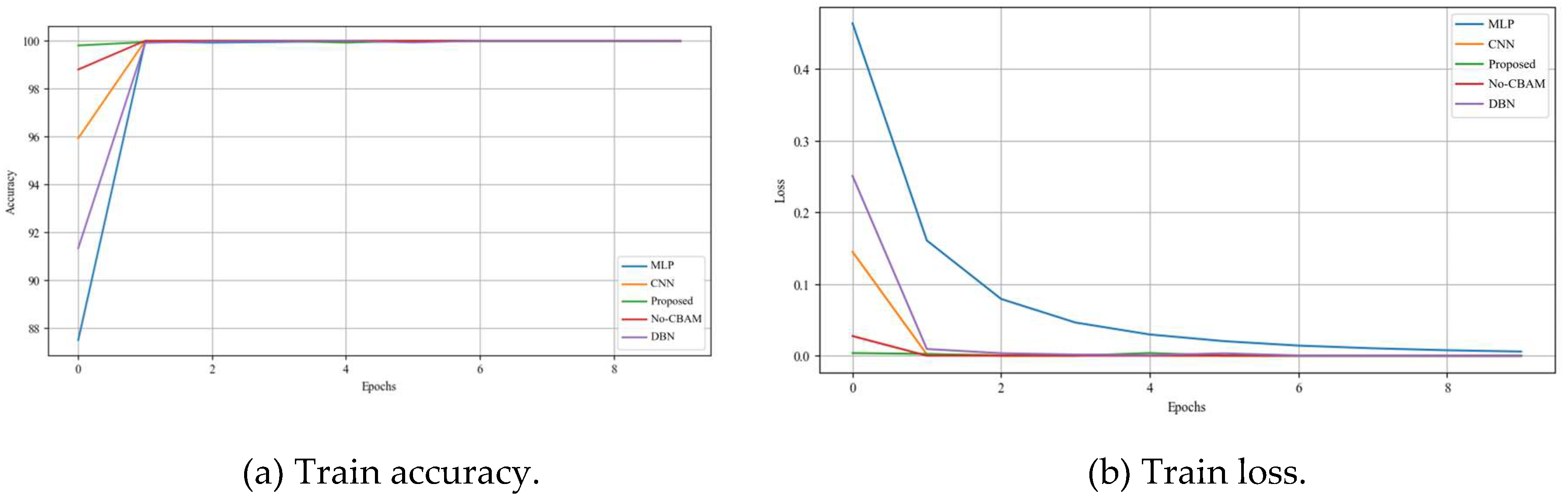
Figure 10.
Compare and contrast the bar graphs of the experimental results.
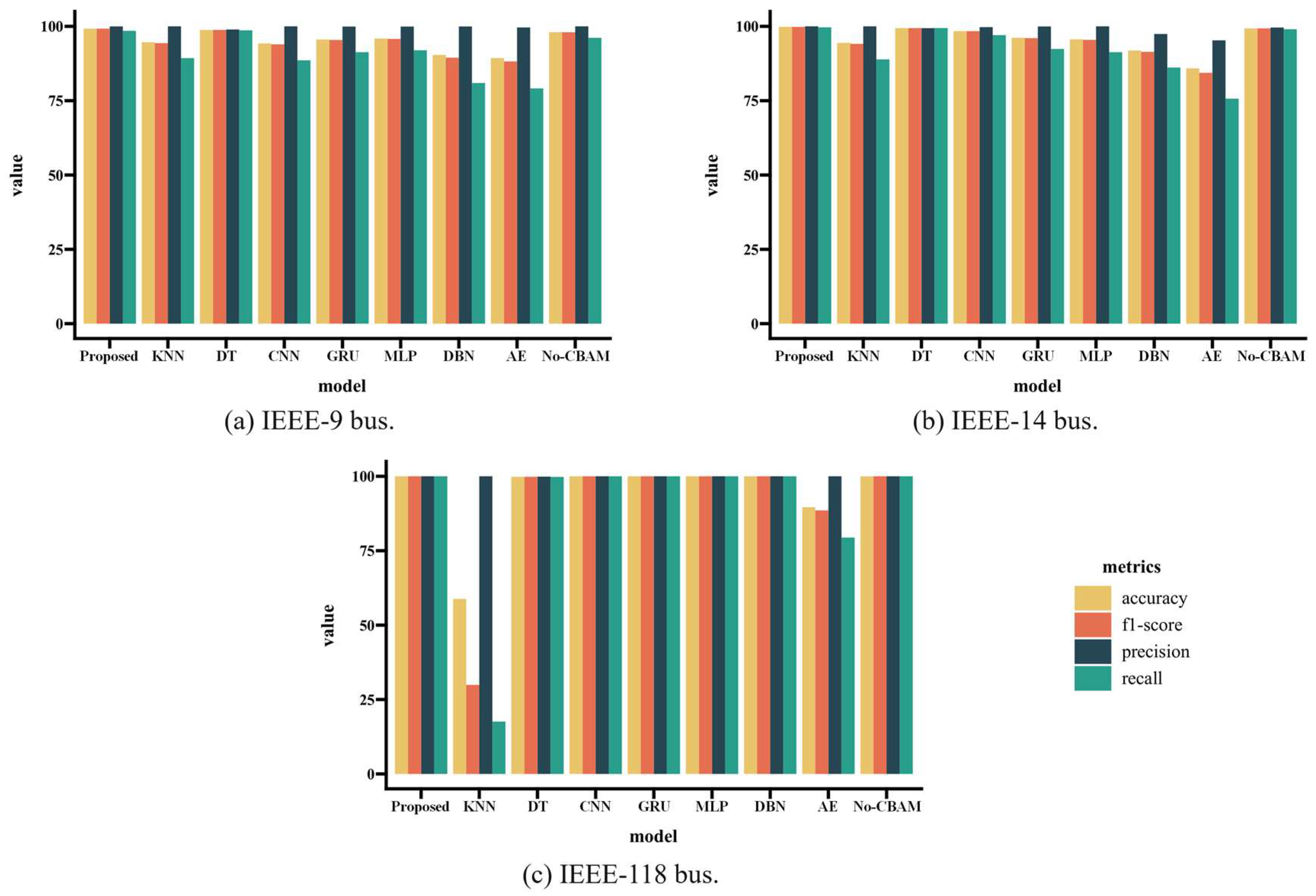
Figure 11.
Heatmap of the extracted features on IEEE-9 bus.
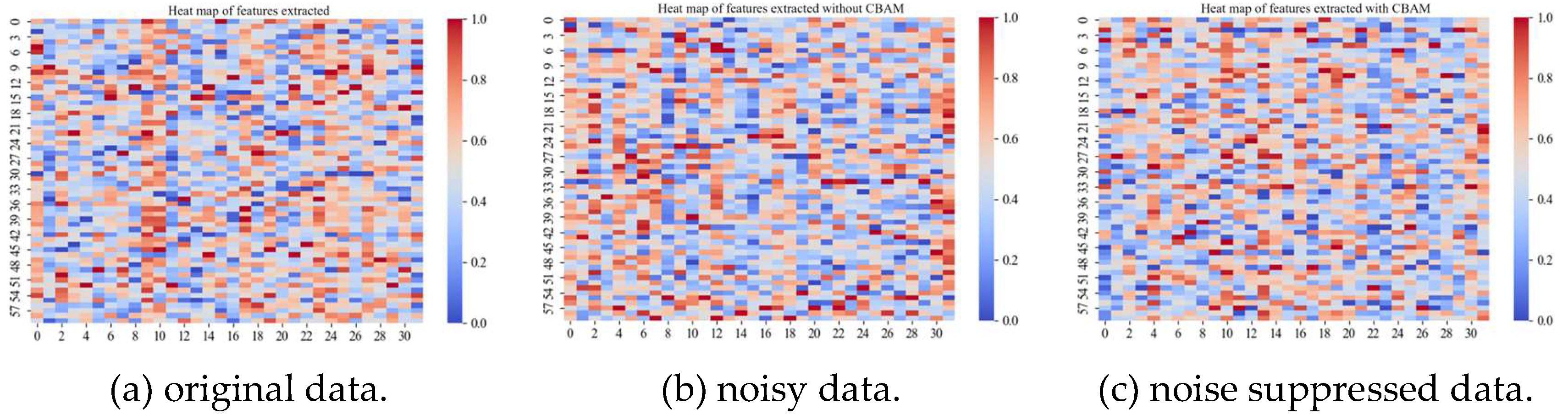
Figure 12.
Heatmap of the extracted features on IEEE-14 bus.
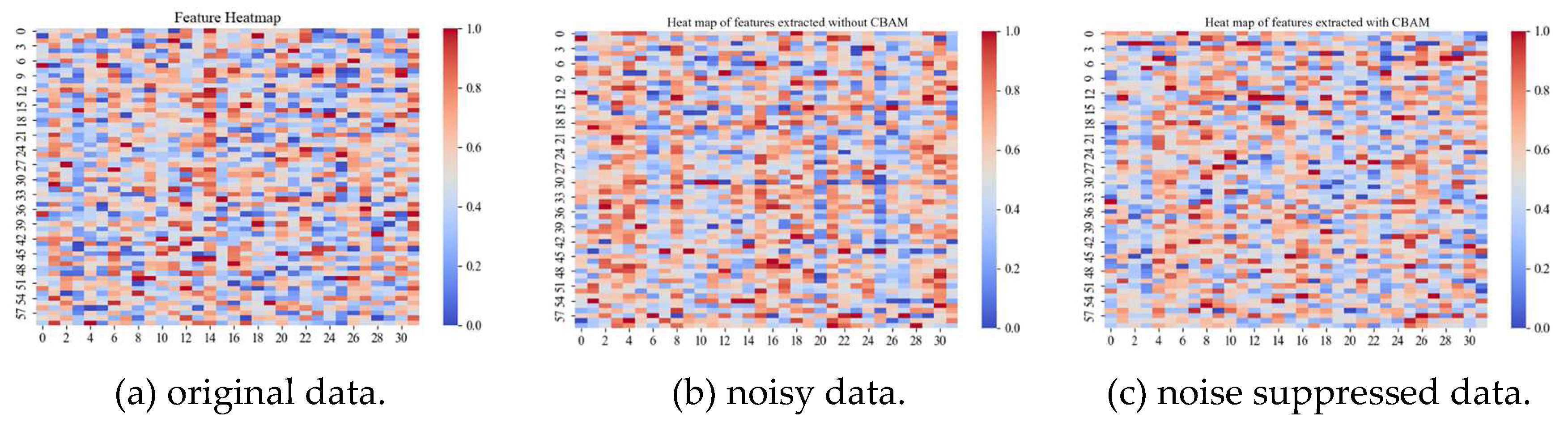
Figure 13.
Heatmap of the extracted features on IEEE-118 bus.
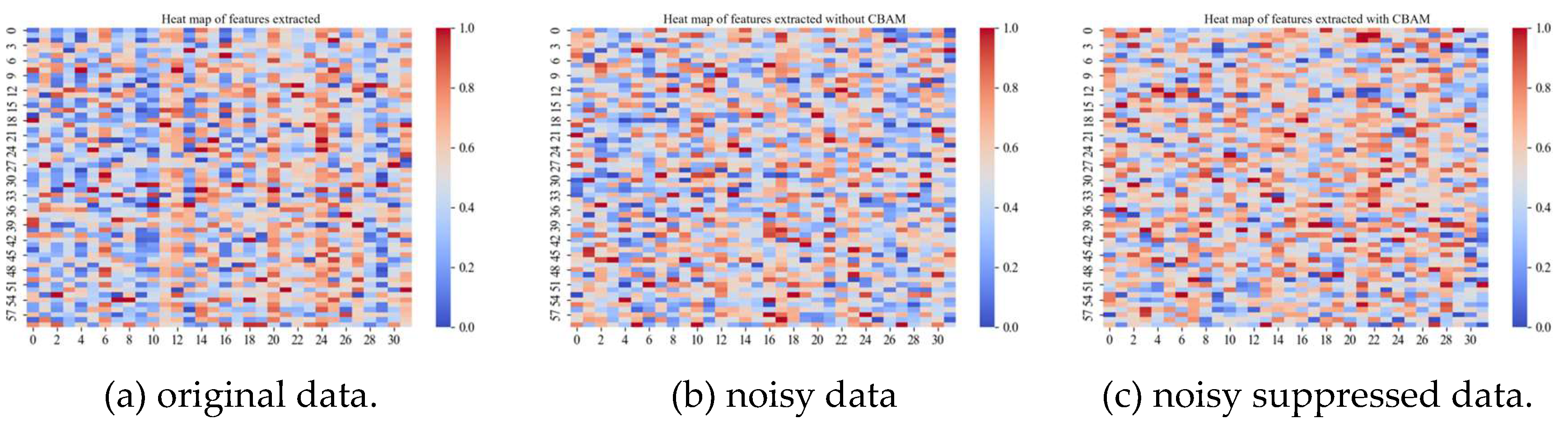
Figure 14.
Accuracy of different noise levels.
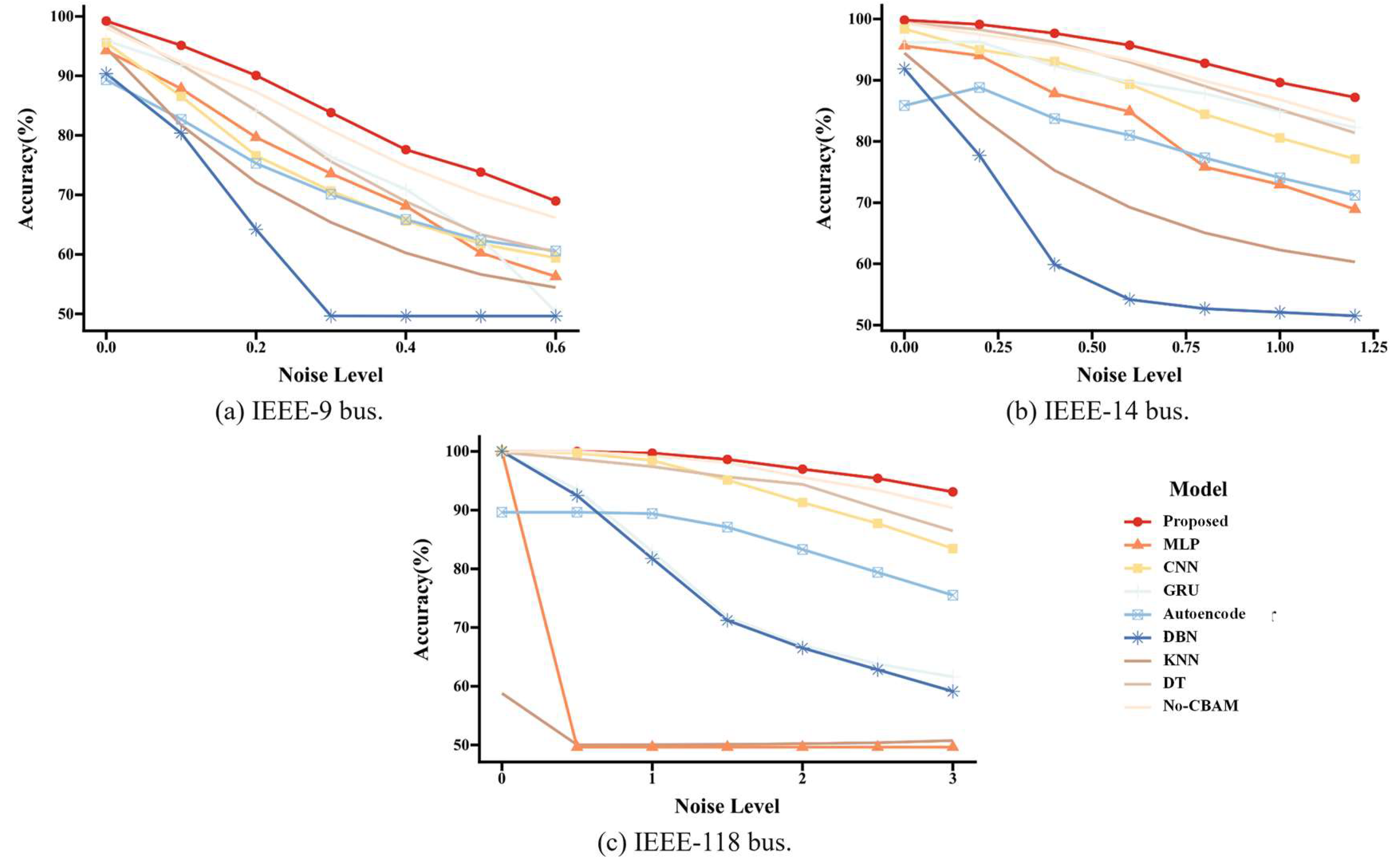
Table 1.
The main system parameters of the test case.
| name | Column | Description |
|---|---|---|
| bus | PD | real power demand |
| QD | reactive power demand | |
| generator | PG | real power output |
| QG | reactive power output | |
| branch | PF | real power injected at “from” bus end |
| QF | reactive power injected at “from” bus end |
Table 2.
The number of measurements of the measurement data.
| Test case | Type | Number | Total |
|---|---|---|---|
| IEEE-9 bus | 9 (9 buses) | 36 | |
| 9 (9 buses) | |||
| 9 (9 branch) | |||
| 9 (9 branch) | |||
| IEEE-14 bus | 14 (14 buses) | 68 | |
| 14 (14 buses) | |||
| 20 (20 branch) | |||
| 20 (20 branch) | |||
| IEEE-118 bus | 118 (118 buses) | 608 | |
| 118 (118 buses) | |||
| 186 (186 branch) | |||
| 186 (186 branch) |
Table 4.
Comparative experimental results in ideal environment.
| System | Method | Accuracy | Precision | Recall | F1-Score |
|---|---|---|---|---|---|
| IEEE-9 bus | Proposed | 99.22 | 99.97 | 98.48 | 99.22 |
| KNN | 94.65 | 100.00 | 89.31 | 94.35 | |
| DT | 98.80 | 98.95 | 98.66 | 98.80 | |
| MLP | 94.25 | 100.00 | 88.58 | 93.95 | |
| CNN | 95.58 | 99.93 | 91.30 | 95.42 | |
| GRU | 95.92 | 99.93 | 91.96 | 95.78 | |
| DBN | 90.38 | 99.96 | 80.94 | 89.45 | |
| AE | 89.33 | 99.62 | 79.12 | 88.20 | |
| No-CBAM | 98.05 | 100.00 | 96.13 | 98.03 | |
| IEEE-14 bus | Proposed | 99.83 | 100.00 | 99.67 | 99.83 |
| KNN | 94.44 | 100.00 | 88.88 | 94.11 | |
| DT | 99.40 | 99.38 | 99.42 | 99.40 | |
| MLP | 95.62 | 100.00 | 91.30 | 95.45 | |
| CNN | 98.38 | 99.73 | 97.05 | 98.37 | |
| GRU | 96.15 | 99.96 | 92.39 | 96.03 | |
| DBN | 91.87 | 97.42 | 86.14 | 91.43 | |
| AE | 85.87 | 95.29 | 75.68 | 84.36 | |
| No-CBAM | 99.32 | 99.60 | 99.04 | 99.32 | |
| IEEE-118 bus | Proposed | 100.00 | 100.00 | 100.00 | 100.00 |
| KNN | 58.80 | 100.00 | 17.58 | 29.90 | |
| DT | 99.84 | 99.89 | 99.79 | 99.84 | |
| MLP | 100.00 | 100.00 | 100.00 | 100.00 | |
| CNN | 100.00 | 100.00 | 100.00 | 100.00 | |
| GRU | 100.00 | 100.00 | 100.00 | 100.00 | |
| DBN | 100.00 | 100.00 | 100.00 | 100.00 | |
| AE | 89.63 | 100.00 | 79.42 | 88.53 | |
| No-CBAM | 100.00 | 100.00 | 100.00 | 100.00 |
Table 5.
The Value of σ under the different datasets.
| Dataset | λ (Noise level) | ||||||
|---|---|---|---|---|---|---|---|
| IEEE-9 bus | 0 | 0.1 | 0.2 | 0.3 | 0.4 | 0.5 | 0.6 |
| IEEE-14 bus | 0 | 0.2 | 0.4 | 0.6 | 0.8 | 1.0 | 1.2 |
| IEEE-118 bus | 0 | 0.5 | 1.0 | 1.5 | 2.0 | 2.5 | 3.0 |
Disclaimer/Publisher’s Note: The statements, opinions and data contained in all publications are solely those of the individual author(s) and contributor(s) and not of MDPI and/or the editor(s). MDPI and/or the editor(s) disclaim responsibility for any injury to people or property resulting from any ideas, methods, instructions or products referred to in the content. |
© 2024 by the authors. Licensee MDPI, Basel, Switzerland. This article is an open access article distributed under the terms and conditions of the Creative Commons Attribution (CC BY) license (http://creativecommons.org/licenses/by/4.0/).
Copyright: This open access article is published under a Creative Commons CC BY 4.0 license, which permit the free download, distribution, and reuse, provided that the author and preprint are cited in any reuse.


