
Submitted:
11 November 2024
Posted:
13 November 2024
You are already at the latest version
Abstract
During daylight laser polarization sensing of high-level clouds (HLCs), the lidar receiving system generates a signal caused by not only backscattered laser radiation, but also scattered solar radiation, the intensity and polarization of which depends on the Sun’s location. If a cloud contains spatially oriented ice particles, then it becomes anisotropic, that is, the coefficients of directional light scattering of such a cloud depend on the Sun’s zenith and azimuth angles. In this work, the possibility of using the effect of anisotropic scattering of solar radiation on the predictive ability of machine learning algorithms in solving the problem of predicting the HLC backscattering phase matrix (BSPM) was evaluated. The hypothesis that radiation scattered on HLCs has no effect on the BSPM elements of such clouds determined with a polarization lidar was tested. The operation of two algorithms for predicting the BSPM elements is evaluated. To train the first one, meteorological data were used as input parameters; for the second algorithm, the azimuthal and zenith angles of the Sun's position were added to the meteorological parameters. It is shown that there is no significant improvement in the predictive ability of the algorithm.
Keywords:
high-level clouds (HLCs)
; polarization lidar
; backscattering phase matrix (BSPM)
; Sun’s azimuthal and zenith angles
; scattered solar radiation
; cloud microphysics
; machine learning (ML)
; random forest
1. Introduction
The study of atmospheric processes is crucial for understanding environmental change, predicting climate variations, and developing strategies to mitigate the effects of dangerous natural phenomena. To this day, despite significant advances in atmospheric science, many aspects of the atmosphere's behavior remain poorly understood due to its complexity. The process of identifying connections between atmospheric characteristics and external factors affecting its state is a challenging and multidimensional task [1,2]. Lidar (Light Identification, Detection, and Ranging) systems are a powerful tool for remote sensing of aerosol formations in the atmosphere including high-level clouds (HLCs). However, processing and interpreting lidar data often requiring complex analysis methods. In this context, it is relevant to consider the use of machine learning (ML) techniques for processing the data of the experiments on remote sensing of natural environment, as well as for solving inverse problems in atmospheric physics, ecology and etc. These methods allow detecting and investigating of interrelationships between various parameters in large volumes of data that would be difficult to identify through classical statistical analysis [3,4,5,6].
The solar radiation flux reaching the Earth's surface is formed by a combination of direct and scattered components. Scattered radiation is formed as a result of interaction between direct solar radiation and atmospheric gases (molecular scattering), water droplets in clouds and fog, ice crystals in clouds, and aerosol particles. Most of the solar radiation energy that reaches the Earth's surface is in the short-wavelength region of the solar spectrum, with wavelengths ranging from approximately 300 to 4,000 nm [7]. The scattered radiation flux depends on the transparency of the atmosphere and is primarily determined by the number of clouds in the sky and their optical and microphysical properties. Aerosol particles in the atmosphere affect the Earth's radiation budget. They can scatter and absorb radiation, directly changing the amount of radiation reaching a particular location. In addition, aerosol particles indirectly affect the Earth’s radiation budget, acting as condensation nuclei of water vapor and, thereby, accelerating the process of cloud formation [8]. Under clear weather conditions, scattered radiation accounts for approximately 15–20% of the total radiation in warm and cold weather [9].
The relationship between the energy flow of solar radiation entering the Earth's surface and the transparency of the atmosphere is being studied by the world scientific community due to the fact that a change in the Earth’s radiation budget may indicate increased air pollution associated with increasing anthropogenic emissions, which leads to changes in weather in certain regions of the Earth and global climate [10]. For example, in [11], the characteristics of solar radiation in the surface layer of the atmosphere were studied under various air pollution conditions over Nanjing, China. The change in the flow of solar radiation affects the surface temperature, the processes of evaporation and condensation of water vapor, the water cycle and, in general, the Earth's ecosystem [12]. Cirrus clouds have less effect on the transmission of direct solar radiation compared to other clouds due to their insignificant optical thickness. At the same time, the large horizontal extent of such clouds, which takes values up to a thousand kilometers [13], as well as the presence of horizontally oriented ice particles in the ice significantly affect the fluxes of scattered solar radiation. A noticeable decrease in the flux of scattered solar radiation in the near-zenith region of the sky by HLC specular areas compared with non-specular areas of the same cloud was first established in experiments on laser polarization sensing of the HLCs by a ground-based lidar oriented in the "zenith" direction [14]. This phenomenon is observed even when the optical thickness of the specular area of the cloud is less than the non-specular one.
The article [15] employed ML tools to investigate the correlation between HLC BSPM elements and meteorological conditions. It is well known, however, that the type of clouds and the Sun’s altitude above the horizon have a significant impact on the flow of radiation coming to the Earth's surface, for example, in the Arctic [16,17]. Consequently, a hypothesis has been proposed regarding the independence of HLC BSPM elements determined during polarization laser sensing experiments on atmospheric polarization from the Sun’s zenith and azimuthal angles. During nighttime, the Sun is absent from the sky entirely, and during daytime, its effect is mitigated by correcting lidar signals against the background noise. The methodological aspects of evaluating the strength of a lidar signal originating from clouds amidst background interference from the "daytime sky" have been elucidated in [18,19]. The purpose of this work was to examine the effect of scattered solar radiation, which depends on the Sun’s zenith and azimuth angles, on the performance of the algorithms used in the work [15]. The next sections describe the experimental setup, data collection, and analysis methods used in this study.
2. Materials and Methods
The data on HLC BSPM for this study were collected using the high-altitude matrix polarization lidar (HAMPL) developed at the National Research Tomsk State University (NR TSU) [20]. The measurements have been performed from 2009 to 2024. To assess the meteorological situation at the altitudes of the examined clouds, data from the ERA5 reanalysis of the European Centre for Medium-Range Weather Forecasts were used. The lidar is located in Tomsk and is oriented vertically in the zenith direction. The HAMPL block diagram is shown in Figure 1.
The HAMPL design is equipped with a Nd:YAG laser operating at a wavelength of 532 nm with a pulse energy of up to 400 mJ, and a pulse repetition rate of 10 Hz, which is used as an optical radiation source. A Cassegrain mirror lens with a primary mirror diameter of 0.5 m and a focal length of 5 m is used as a receiving antenna. The lidar receiving system includes the ThorLabs FL532-1 interference filter with a central wavelength of 532 ± 0.6 nm and a half-width of the transmission spectrum of 3 ± 0.6 m. Then the Wollaston prism, which divides received backscattered radiation into two orthogonally polarized beams. These radiation beams are registered with two photomultiplier tubes (PMTs) operating in the photon-counting mode with time strobing of the signal, which provides the altitude resolution from 37.5 to 150 m [21]. To suppress active backscattering interference from the near lidar zone (up to 3 km), electro-optical shutters (EOSs) based on a potassium dideuterium phosphate (DKDP) crystal are installed in front of the PMTs. The use of EOSs allows the PMT characteristics to be to maintained linear even during lidar operation in the daytime with the maximum energy of the probing pulse.
During each sensing cycle, pulses of radiation with four different polarization states (three linear and one circular) were sent to the atmosphere one by one. For each pulse, the polarization state of backscattered radiation described by the Stokes vector was determined. Thus, 16 intensity vertical profiles, from which 16 BSPM elements were calculated, were measured in each sensing cycle. The HAMPL provided the registration of lidar returns from HLC in the parallel accumulation mode of 16 arrays of single-electron pulses. This mode allowed the intensity of all 16 lidar signals from the clouds, which were necessary to determine all elements of the BSPM, to be estimated with the same error. During sensing in this mode, there was a continuous change of polarization elements in the transmitting and receiving systems of the lidar, due to which the minimum time of a complete cycle of measurements for determining all BSPM elements was 2 s. Thus, the movement of the examined air volumes falling into the field of view of the telescope affected the measurements in the same way with each of the used combinations of the polarization states of sensing and received radiation [20,21]. Lidar signal processing is based on the application of the laser sensing equation (LSE). In vector form [22] of this equation:
where P(z) and s(z) are the power and the normalized Stokes vector parameter of radiation incident on the input of the lidar receiving system from the scattering volume located on the sensing path at a distance z from the source, respectively; c is the speed of light in the medium; W0 = P0Δt is the pulse energy of the lidar transmitter (P0 and Δt are the power and duration of the laser pulse, respectively); A is the effective area of the receiving antenna; G(z) is the geometric factor (when sensing high-level clouds, G(z) is usually equals to 1); Mπ(z) is the normalized BSPM of the scattering volume; s0 is the normalized Stokes vector parameter of sensing radiation; ε(z',θ,φ) is the attenuation coefficient; θ and φ are the polar and azimuthal angles, respectively. It should be taken into account that the LSE in this form does not take into account the dependence of the radiation attenuation on the propagation direction relative to the axes characterizing the medium anisotropy. Also excluded from consideration is the possible change in the polarization state of direct and scattered radiation as it passes through a section of the sensing path located in an anisotropic medium. Note that the P(z) is corrected for the background noise, i.e., its value here is subtracted from the initially measured value.
Special attention should be paid to the characteristics of the examined clouds, which are determined in lidar measurements. The key among them is the BSPM, which mathematically is the operator of the transformation of the Stokes vector parameter describing the polarization state of sensing radiation and the Stokes vector parameter of backscattered radiation received with the lidar. The effect of the scattering volume on the polarization state of radiation is determined by the parameters of its microstructure: the parameters of the distributions of solid particles in clouds in shape, size, and spatial orientation. In other words, physically, the BSPM contains information about the cloud microstructure. Separately, we focus the reader's attention on the fact that each BSPM element is determined by the ratios of the components of the Stokes vector parameter of received radiation for various polarization states of sensing radiation. At the same time, to determine these components, not pure linear signals or even just lidar signals minus the background level are used, but also their ratios. Thus, the possible effect of the background noise on the BSPM elements is not explicitly present, and, taking into account the background level at the early stages of lidar signal processing, we exempt from its effect the HLC optical characteristics obtained in the lidar experiment.
The NR TSU HAMPL is located in the southern part of Tomsk (56°26' N 84°58' E), about 0.5 km from the bank of the Tom’ River. Measurements are performed in the absence of low clouds, precipitation and gusty winds. The duration of one series of lidar measurements is usually 16 minutes and 40 seconds. The description of the distributions of the number of lidar measurements and the number of cases of HLC registration in them by year and season was previously published [20,21]. To evaluate the meteorological conditions at the altitudes of the examined clouds, we relied on data from the ERA5 reanalysis provided by the European Centre for Medium-range Weather Forecasts [21]. The most reliable source of data on the vertical profiles of meteorological parameters is radiosonde observations, although the nearest stations to Tomsk where radiosonde launches are performed regularly are approximately 200–230 kilometers away (Kolpashevo and Novosibirsk). Although the meteorological conditions at the altitudes of cloud formation in the upper atmosphere are usually similar according to these data, the ERA5 reanalysis offers a higher temporal resolution (1 hour compared to 12 hours). With a high spatial resolution (30 × 30 km), the ERA5 reanalysis allows access to the vertical profiles of the meteorological parameters and Tomsk coordinates [23]. As initial data for the ERA5, measurements from various sources around the globe are used: satellite radiometers, ground-based, ship-based and aircraft weather stations, weather buoys, balloon-borne sensors, and ground-based radars [24]. At the HLC formation altitude, the vertical resolution of the ERA5 data is 25–50 hPa, which is approximately equivalent to 0.5–1 km. To evaluate the meteorological situation at the formation altitudes of the examined clouds, the altitudes of their boundaries are determined based on the lidar measurement data, for which the corresponding reanalysis data are then adjusted by coordinates, date, time, and altitude.
To test the hypothesis that the signals measured during lidar experiments are independent of the zenith and azimuth angles of the Sun’s position, these angles were calculated using a similar method as described in [25]. The input parameters for the calculations included the coordinates and time zone of the observation location, as well as the specific date and time of the event. There is a known issue in treating azimuthal and zenith angle values when they approach 360 degrees—a discontinuity, which can cause errors in program calculations due to the large numerical difference between angles that are essentially adjacent. For example, the angles 359° and 1° are mathematically close, but their direct numerical representation introduces a sharp transition, leading to inconsistencies when performing trigonometric calculations. We converted the angular values into a continuous form by calculating their sine and cosine components to ensure that angles, which are next to each other on a circular scale, are handled consistently by the algorithms. Four continuous variables from the sine and cosine of both the azimuthal and zenith angles were computed and then used in the analysis.
In a previous study [15], the relationship between the HLC BSPM elements and altitude was investigated, with results showing no significant correlation. Based on these results, in this study, for each set of lidar measurements, the median values from the experimental sample were used as the values for the BSPM elements. The article [15] also demonstrates that only the elements on the matrix main diagonal (m22, m33, and m44) have a specific dependence on meteorological variables. The block diagram of our methodology is shown in Figure 2.
As previously mentioned, a dataset used in this research has been generated from the median values of BSPM elements and their associated date, time, coordinates, and altitude values for meteorological parameters based on the ERA5 data [26]. This dataset was then enhanced by including the sine and cosine values of the Sun's azimuth and zenith angles. After that, machine learning models were trained using two versions of the dataset: one containing only meteorological data, and the other incorporating solar position data. Next, the results of the trained models were evaluated and compared using a held-out sample. Random Forest (RF) models were used, including a version with data preprocessing using principal component analysis (RF+PCA). Validation sample that was held out used to assess the accuracy of the models' forecasts for HLC characteristics was generated from data covering the period from February 15, 2020, to September 22, 2023 (65 observations). This validation set was not used during the training phase, allowing for an unbiased assessment of the model's ability.
3. Results
After training the ML algorithms, the validation dataset was used to assess the accuracy of the models in predicting the BSPM elements. In the process of choosing the optimal algorithms for predicting the values of the BSPM elements, all possible variants of the number of components in the PCA method were investigated. The best results in terms of the predictive ability of the algorithms were obtained on the data processed using PCA with the number of components equal to 9 and 15. The number of possible components varies from 1, which is necessary for the presence of at least one training feature, to the total number of available features, which is 65, among which 5 meteorological values collected at 13 different altitudes.
The performance of the models trained on two datasets—one including solar data and one without them—was compared using a metric in the form of a mean squared error (1). This metric was calculated between the values predicted by the algorithm and the actual experimental data. The results are presented in Table 1. RF stands for the random forest algorithm, while PCA represents the data that has been preprocessed using the principal component analysis (the number of components used is indicated in parentheses).
The "Percentage of improvement" column provides a quantitative description of the correspondence of the HLC BSPM elements predicted by machine learning methods actually obtained during lidar measurements using the two mentioned data sets.
4. Discussion
As can be observed from Table 1, there has been no significant and consistent improvement in the performance of any of the algorithm types. There are minor differences in the algorithm's output when comparing results without the use of the Sun’s zenith and azimuth angles compared to those with them. Although the estimated improvements are up to several percent, the differences in the results obtained using both methods are small (0.0001–0.001). Therefore, even significant differences in the percentage of improvement among the three machine learning techniques used, which amount to a few percent, are not explainable from the perspective of atmospheric optics. The results obtained suggest that the inclusion of the Sun's zenith and azimuth angle in the experimental dataset used to train the machine learning models does not significantly impact their predictive ability when searching for correlations between HLC BSPM elements and meteorological parameters. However, this conclusion is tentative. It may be related to the method of post-detection processing of the lidar signal. This process involves the following steps: from the stream of received total lidar signal (consisting of both useful and interfering signals), the interfering signal, which contain a flow of direct solar radiation scattered by HLC, is subtracted.
4. Conclusions
In the present work, a random forest algorithm is considered to determine the dependence of the HLC BSPM elements determined in the experiments on polarization laser sensing of the atmosphere on the measurement parameters. Previously, meteorological parameters and the Sun’s zenith and azimuth were considered as measurement parameters. A hypothesis was formulated and verified about the absence of an effect of the Sun's position on the signals measured in lidar experiments, and, consequently, on the predicted BSPM elements. The results demonstrated that the inclusion of the Sun’s angles did not lead to significant or consistent improvements in the prediction of BSPM elements. In several cases, we have observed that algorithms using solar data as an input parameter may experience a degradation in their predictive capabilities. For example, when using the RF+PCA (15) algorithm to predict the m33 element, we observed a degradation of 6.47%. At the same time, if the algorithms were to improve their performance, it would not be by more than 1.5%. It was concluded that, in general, there is no significant tendency for the Sun’s angles to affect the algorithm's predictive ability. These findings support the initial hypothesis that the Sun's azimuth and zenith angles do not significantly influence the accuracy of lidar-based cloud measurements.
5. Patents
The research was carried out with the support of a grant from the Government of the Russian Federation (Agreement No. 075-15-2024-667 of 23 August 2024) in the part of the potential of using the effect of anisotropic solar radiation scattering on the prediction accuracy of machine learning models for predicting the elements of backscattering phase matrix (BSPM) of HLC was explored. This research was funded by the Russian Science Foundation, Grant No. 24-72-10127 in the part of studying the relationship between the optical, microphysical, and geometric characteristics of high-level clouds with predominantly horizontally oriented ice particles and the meteorological conditions leading to their formation and evolution.
Author Contributions
(O.K.), (I.B.), and (M.P.) developed the idea of this work. (I.S.) and (I.B.) conducted a preliminary analysis and interpretation of lidar and meteorological data. (O.K.), and (M.P.) developed a software product using machine learning tools for analyzing meteorological observation data and predicting optical and geometric characteristics of the HLC. (I.A.) and (D.R.) programmatically compared two approaches to learning algorithms (with and without solar data) for predicting HLC BSPM elements. (E.V.) and (I.Zh.) performed experiments on lidar sensing of the atmosphere. (I.B.), (M.P.), (O.K.), and (I.S.) analyzed the measurement and calculated data. (I.B.), (M.P.), (O.K.), (I.S.), (I.A.), and (D.R.) discussed the results, wrote, and edited the article.
References
- Wilson, L.; Goh, T.T.; Chung Wang, W.Y. Big Data in Climate Change Research: opportunities and Challenges. International Journal of E-Adoption (IJEA) 2020, 4, 1–14. [Google Scholar] [CrossRef]
- Isaksen, I.S.A.; Granier, C.; Myhre, G.; Berntsen, T.K.; Dalsøren, S.B.; Gauss, M.; Klimont, Z.; Benestad, R.; Bousquet, P.; Collins, W.; Cox, T.; Eyring, V.; Fowler, D.; Fuzzi, S.; Jöckel, P.; Laj, P.; Lohmann, U.; Maione, M.; Monks, P.; Prevot, A.S.H.; Raes, F.; Richter, A.; Rognerud, B.; Schulz, M.; Shindell, D.; Stevenson, D.S.; Storelvmo, T.; Wang, W.-C.; van Weele, M.; Wild, M.; Wuebbles, D. Atmospheric composition change: Climate–Chemistry interactions. Atmospheric Environment 2009, 43, 5138–5192. [Google Scholar] [CrossRef]
- Wilks, D.S. Statistical Methods in the Atmospheric Sciences, International Geophysics Series, 2nd ed.; Academic Press: USA, 2006; 627p. [Google Scholar]
- Lapčák, M.; Ovseník, Ľ.; Oravec, J.; Zdravecký, N. Investigation of Machine Learning Methods for Prediction of Measured Values of Atmospheric Channel for Hybrid FSO/RF System. Photonics 2022, 9, 524. [Google Scholar] [CrossRef]
- Ukkonen, P. Exploring Pathways to More Accurate Machine Learning Emulation of Atmospheric Radiative Transfer. Journal of Advances in Modeling Earth Systems 2022, 14, e2021MS002875. [Google Scholar] [CrossRef]
- Veerman, M.A.; Robert, P.; Robin, S.; van Leeuwen, C.M.; Damian, P.; van Heerwaarden, C.C. Predicting atmospheric optical properties for radiative transfer computations using neural networks. Philosophical Transaction A 2021, 379, 20200095. [Google Scholar] [CrossRef] [PubMed]
- Guide on actinometric observations for hydrometeorological stations, 3rd ed.; Gidrometeoizdat: Leningrad, USSR, 1973. (In Russian)
- Andrews, E.; Ogren, J.A.; Bonasoni, P.; Marinoni, A.; Cuevas, E.; Rodríguez, S.; Sun, J.Y.; Jaffe, D.A.; Fischer, E.V.; Baltensperger, U.; Weingartner, E.; Collaud Coen, M.; Sharma, S.; Macdonald, A.M.; Leaitch, W.R.; Lin, N.-H.; Laj, P.; Arsov, T.; Kalapov, I.; Jefferson, A.; Sheridan, P. Climatology of aerosol radiative properties in the free troposphere. Atmospheric Research 2011, 102, 365–393. [Google Scholar] [CrossRef]
- Abakumova, G.M.; Gorbarenko, E.V. Transparency of the atmosphere in Moscow over the past 50 years and its changes in Russia; LKI Publishing House: Moscow, Russia, 2008. (In Russian) [Google Scholar]
- Liepert, B.G. Observed reductions of surface solar radiation at sites in the United States and worldwide from 1961 to 1990. Geophys. Res. Let. 2002, 29, 61. [Google Scholar] [CrossRef]
- Luo, H.; Han, Y.; Lu, C.; Yang, J.; Wu, Y. Characteristics of Surface Solar Radiation under Different Air Pollution Conditions over Nanjing, China: Observation and Simulation. Advances in Atmospheric Sciences 2019, 36, 1047–1059. [Google Scholar] [CrossRef]
- Haverkort, A.J.; Uenk, D.; van der Waart, M. Relationships between ground cover, intercepted solar radiation, leaf area index and infrared reflectance of potato crops. Potato Research 1991, 34, 113–121. [Google Scholar] [CrossRef]
- Feigelson, E.M. (Ed.) Radiation Properties of Perispheric Clouds; Nauka: Moscow, USSR, 1989. (In Russian) [Google Scholar]
- Bryukhanov, I.D.; Zuev, S.V.; Samokhvalov, I.V. Effect of specular high-level clouds on scattered solar radiation fluxes at the zenith. Atmospheric and Oceanic Optics 2021, 34, 327–334. [Google Scholar] [CrossRef]
- Kuchinskaia, O.; Penzin, M.; Bordulev, I.; Kostyukhin, V.; Bryukhanov, I.; Ni, E.; Doroshkevich, A.; Zhivotenyuk, I.; Volkov, S.; Samokhvalov, I. Artificial Neural Networks for Determining the Empirical Relationship between Meteorological Parameters and High-Level Cloud Characteristics. Applied Sciences 2024, 14, 1782. [Google Scholar] [CrossRef]
- Minnett, P.J. The Influence of Solar Zenith Angle and Cloud Type on Cloud Radiative Forcing at the Surface in the Arctic. Journal of Climate 1999, 12, 147–158. [Google Scholar] [CrossRef]
- Bai, J.; Zong, X. Global Solar Radiation Transfer and Its Loss in the Atmosphere. Applied Sciences 2021, 11, 2651. [Google Scholar] [CrossRef]
- Kaul, B.V.; Volkov, S.N.; Samokhvalov, I.V. Studies of ice crystal clouds through lidar measurements of backscattering matrices. Atmospheric and Oceanic Optics 2003, 16, 325–332. [Google Scholar]
- Volkov, S.N.; Kaul, B.V.; Samokhvalov, I.V. A technique for processing lidar measurements of backscattering matrices. Atmospheric and Oceanic Optics 2002, 15, 891–895. [Google Scholar]
- Bryukhanov, I.D.; Kuchinskaia, O.I.; Ni, E.V.; Penzin, M.S.; Zhivotenyuk, I.V.; Doroshkevich, A.A.; Kirillov, N.S.; Stykon, A.P.; Bryukhanova, V.V.; Samokhvalov, I.V. Optical and Geometrical Characteristics of High-Level Clouds from the 2009–2023 Data on Laser Polarization Sensing in Tomsk. Atmospheric and Oceanic Optics 2024, 37, 343–351. [Google Scholar] [CrossRef]
- Kuchinskaia, O.; Bryukhanov, I.; Penzin, M.; Ni, E.; Doroshkevich, A.; Kostyukhin, V.; Samokhvalov, I.; Pustovalov, K.; Bordulev, I.; Bryukhanova, V.; Stykon, A.; Kirillov, N.; Zhivotenyuk, I. ERA5 Reanalysis for the Data Interpretation on Polarization Laser Sensing of High-Level Clouds. Remote Sensing 2023, 15, 109. [Google Scholar] [CrossRef]
- Kaul, B.V. Optical-Location Method of Polarization Studies of Anisotropic Aerosol Media. Doctor’s Dissertation in Physical-Mathematical Sciences, Tomsk, 2004. [Google Scholar]
- ECMWF Reanalysis v5 (ERA5). Available online: https://www.ecmwf.int/en/forecasts/dataset/ecmwf-reanalysis-v5 (accessed on 19 September 2024).
- ECMWF Confluence Wiki. ERA5: data documentation. Available online: https://confluence.ecmwf.int/display/CKB/ERA5%3A+data+documentation#ERA5:datadocumentation-Introduction (accessed on 19 September 2024).
- Rizvi, A.A.; Addoweesh, K.; El-Leathy, A.; Al-Ansary, H. Sun position algorithm for sun tracking applications. In Proceedings of the IECON 2014—40th Annual Conference of the IEEE Industrial Electronics Society, Dallas, TX, USA; 2014; pp. 5595–5598. [Google Scholar] [CrossRef]
- Copernicus Climate Data Store. Available online: https://cds.climate.copernicus.eu (accessed on 19 September 2024).
Figure 1.
HAMPL: a) block diagram: 1—laser; 2—Glan–Taylor prism; 3—collimator; 4—stepper motor; 5—polarization transformation unit; 6—Cassegrain telescope; 7—field stop; 8—lens; 9—interference filter; 10—Wollaston prism; 11—PMTs; 12—EOSs; 13—computer-based data recording and displaying equipment [21]; b) view of the receiving and transmitting part; c) view on the roof of the building; d) view from the roof of the building.
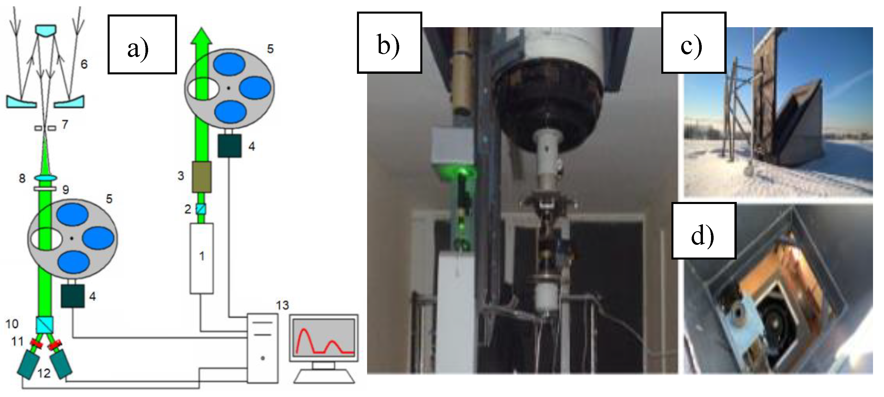
Figure 2.
Methodology for collecting the experimental data and using them to predict the HLC BSPM elements.
Figure 2.
Methodology for collecting the experimental data and using them to predict the HLC BSPM elements.
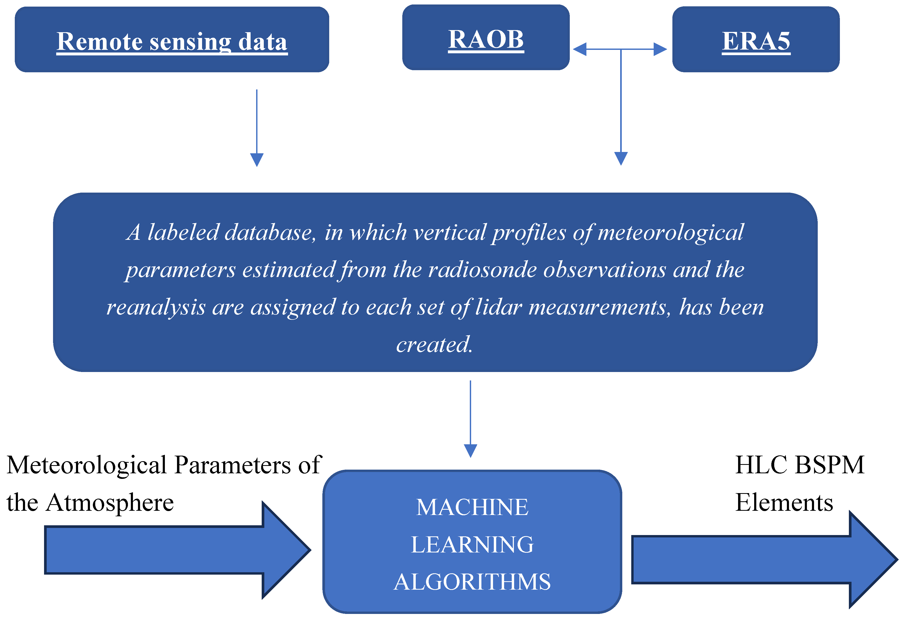

Table 1.
The results of a comparative analysis of the algorithms.
| Method | The predicted HLC BSPM element | The value obtained without using the angles of the Sun's position | The value obtained with using the angles of the Sun's position | Difference | Improvement percentage, % |
|---|---|---|---|---|---|
| RF | m22 | 0.03623 | 0.03635 | –0.00012 | –0.33 |
| m33 | 0.05577 | 0.05551 | 0.00026 | 0.47 | |
| m44 | 0.11618 | 0.11811 | –0.00193 | –1.66 | |
| RF+PCA (15) | m22 | 0.0292 | 0.02851 | 0.00069 | 2.36 |
| m33 | 0.05621 | 0.05968 | –0.00347 | –6.17 | |
| m44 | 0.09536 | 0.09524 | 0.00012 | 0.13 | |
| RF+PCA (9) | m22 | 0.02929 | 0.02887 | 0.00042 | 1.43 |
| m33 | 0.06383 | 0.06355 | 0.00028 | 0.44 | |
| m44 | 0.09547 | 0.09998 | –0.00451 | –4.72 |
Disclaimer/Publisher’s Note: The statements, opinions and data contained in all publications are solely those of the individual author(s) and contributor(s) and not of MDPI and/or the editor(s). MDPI and/or the editor(s) disclaim responsibility for any injury to people or property resulting from any ideas, methods, instructions or products referred to in the content. |
© 2024 by the authors. Licensee MDPI, Basel, Switzerland. This article is an open access article distributed under the terms and conditions of the Creative Commons Attribution (CC BY) license (http://creativecommons.org/licenses/by/4.0/).
Copyright: This open access article is published under a Creative Commons CC BY 4.0 license, which permit the free download, distribution, and reuse, provided that the author and preprint are cited in any reuse.


