Submitted:
11 October 2025
Posted:
13 October 2025
You are already at the latest version
Abstract
The Ozone Monitoring Suite–Limb (OMS-L) carried by the Fengyun-3F (FY-3F) satellite, as China's first effective payload using the limb observation mode to conduct hyperspectral atmospheric detection in the ultraviolet (UV) and visible (Vis) bands, was successfully launched on August 3, 2023. It mainly serves the research in the fields of climate change, atmospheric chemistry, and atmospheric environment. This study is the first to conduct the retrieval of the ozone profiles from OMS-L data. The retrieval scheme utilizes the radiances within the UV band, normalizing them to the radiance at the upper tangent height. To minimize the impact of aerosol scattering, the pair method is implemented, with seven carefully selected wavelength pairs fully exploiting ozone’s UV absorption characteristics. The weighted multiplicative algebraic reconstruction technique (WMART) is then applied to effectively integrate multi-wavelength information, in tandem with an iterative retrieval process using the radiative transfer model. This approach yields ozone concentration profiles in the altitude range of approximately 18-55 km. The retrieval errors resulting from the parameters are estimated to be 5–13% above 25 km, increasing to 10–30% in the upper troposphere. Comparison of OMS-L retrieved ozone profiles with the OMPS/LP v2.6 product reveals good consistency, with differences generally within 10% in the 20-50 km altitude range. However, biases are more pronounced at lower altitudes, particularly in tropical regions. This work conclusively demonstrates that, OMS-L can accurately measure stratospheric ozone profiles with high vertical resolution, thereby contributing significantly to the field of atmospheric science.
Keywords:
ozone profile
; limb sounding
; retrieval
; OMS-L
; OMPS/LP
1. Introduction
Atmospheric ozone is a crucial component of the Earth's atmospheric composition and plays an irreplaceable role in the Earth's ecological and climate systems [1]. Stratospheric ozone can effectively absorb the vast majority of ultraviolet (UV) radiance in solar irradiances, protecting organisms on Earth from excessive UV exposure and being of great significance for maintaining the ecological balance of the Earth [2,3]. Although the academic community currently has a relatively in-depth understanding of the chemical properties of stratospheric ozone, there are still many issues that urgently need to be clarified in aspects such as the recovery of the ozone hole [4,5], the impact of the increase in greenhouse gases on atmospheric circulation and temperature [6], the interaction between stratospheric and tropospheric ozone [7,8], and the long-term change trend of ozone [9].
For example, Kessenich et al. comprehensively analyzed the monthly and daily ozone variations at different altitudes and latitudes within the Antarctic ozone hole, and found that although there were signs of recovery in early spring, the ozone in the middle stratosphere in October has continued to decrease significantly since 2004, highlighting the importance of continuous monitoring and evaluation of the ozone layer [10]. Ardra et al. found unprecedented ozone depletion during the winter and spring seasons in the Arctic in recent years [11]. Ma et al. revealed a new mechanism of stratospheric ozone depletion—the smoke charging vortex caused by wildfires through advanced numerical simulations and satellite observations [12]. Chen et al. quantified for the first time the stratospheric intrusion to the surface (SITS) event using data from ground-based air monitoring stations in China, and analyzed the long-term and short-term effects of stratospheric ozone on the evolution of ground-level ozone concentration in China [13]. Therefore, accurately understanding the vertical distribution of stratospheric ozone is of great value for a deeper understanding of the operating mechanism of the Earth's ecological system, evaluating the impact of climate change on the ecological environment, and formulating effective environmental protection strategies.
The researches on the spatiotemporal dynamics of atmospheric ozone mainly rely on ground-based monitoring [14], model simulation [15], and satellite remote sensing measurements [16]. Compared with ground-based monitoring methods and chemical transport models, satellite remote sensing observation has the advantages of wide coverage, high spatial resolution, and a long time series. The limb sounding technique, which is widely used in recent satellite instruments, combines the advantages of nadir observation and occultation mode. It has a better vertical resolution compared to the nadir geometry and a higher horizontal sampling rate than occultation measurements [17]. Limb sounding techniques can be classified into limb emission and limb scattering according to the wavelength range. In limb emission, the signal emitted by the atmosphere is weak, resulting in a relatively low signal-to-noise ratio; while limb scattering observation use the scattered sunlight and are limited to measurements during daylight [18].
New-generation limb scattering satellite instruments launched by various countries at home and abroad, such as the Scanning Imaging Absorption Spectrometer for Atmospheric Cartography (SCIAMACHY) [19], the Optical Spectrograph and Infrared Imager System (OSIRIS) [20], the Ozone Mapper and Profile Suite Limb Profiler (OMPS/LP) [21], Ozone Monitoring Suite–Limb (OMS-L) [22], and the Backward Limb Spectrometer (BLS) [2], can provide vertical ozone profiles with a high vertical resolution (1-3 km) and global coverage by observing the scattered solar light.
The Fengyun-3F (FY-3F) satellite, an important member of the Fengyun-3 series of China's second-generation low-orbit meteorological satellites, was successfully launched on August 3, 2023, and has been operating stably since then. The Ozone Monitoring Suite–Limb (OMS-L), a payload aboard the satellite, is a newly developed instrument specifically designed for the detection of trace gases such as ozone. It employs the limb sounding technique combined with continuous spectral observation, which is applied for the first time, significantly improving the spectral resolution and spatial resolution. A novel retrieval scheme is developed for retrieving the stratospheric ozone profiles from OMS-L measurements. This retrieval method uses UV wavelength pairing and the weighted multiplicative algebraic reconstruction technique (WMART), and in combination with the radiative transfer model, retrieves the ozone profiles at altitudes ranging from ~18 to 55 km. Moreover, the retrieval results from OMS-L are compared with the OMPS/LP v2.6 ozone profile product. The purpose of this study is to deeply explore the methods and technologies for retrieving the stratospheric ozone profile from OMS-L data and accurately evaluate the accuracy and reliability of the retrieval results.
2. Materials and Methods
2.1. Materials
2.1.1. The OMS-L on FY-3F Satellite
The FY-3F satellite conducts continuous optical and microwave imaging observations of the land-atmosphere system and vertical sounding in the morning. It is a near polar sun synchronous orbit satellite with an average altitude of approximately 836 km, an orbital inclination of about 98.8°, a local time of 10:00-10:20 at the orbital descending node, and an orbital period of around 101.5 minutes.
The FY-3F satellite is equipped with 10 powerful and advanced remote sensing instruments (Figure 1a). Among them, the OMS-L is a newly developed instrument, and also China's first effective payload that uses the limb observation mode to conduct hyperspectral atmospheric detection in the UV and Vis bands (290-500 nm). OMS-L is a spectrometer that adopts the secondary dispersion technology of a prism plus a grating and employs a refrigerated two-dimensional Complementary Metal-Oxide-Semiconductor (CMOS) detector for imaging. The main performance indicators of the instrument are shown in Table 1. The scattered radiances incident on OMS-L instrument are first separated into partially polarized light and linearly polarized light by a Brewster angle polarizer. The partially polarized light, after being processed by a beam splitter, forms images on two CMOS array detectors, thereby generating spectral data of two bands, which are mainly used for atmospheric detection. The linearly polarized light forms an image on the third CMOS array detector, generating the spectrum of the third band, which is used to perform polarization correction for the first two bands [22].
The OMS-L instrument observes the scattering of solar UV and Vis light by the stratosphere through the limb sounding technique, and measures the vertical distribution profiles of trace gases such as global O3, NO2, SO2, BrO, HCHO, and OClO, as well as quantitative and qualitative products of clouds and aerosols. The point of closest approach of the instrument's line of sight (LOS) to the Earth's surface is referred to as the tangent point (TP). The altitude of the TP, after terrain correction via the digital elevation model (DEM), is the tangent height (TH). Figure 1b shows a schematic diagram of the limb geometry.
2.1.2. The OMS-L Level-1 Version 1.2 Data
The OMS-L L1 v1.2 product consists of radiometric spectra generated through a series of processing steps. These steps include decoding, geolocation, bad-pixel detection, dark-current processing, spectral calibration, radiometric calibration, polarization correction, and quality control, all of which are based on the L0 raw data and pre-processed static parameters [22](Li, 2024). As shown in Figure 2a, it displays the available orbits for OMS-L observations on August 1, 2024. The red arrow indicates the satellite's flight direction. With an orbital inclination of 98° relative to the equator, the satellite achieves nearly global coverage, as the corresponding sampling latitude range for the nominal pointing of the orbital instrument spans from 80°S to 80°N. The spacecraft completes 14-15 orbits per day, and the instrument typically conducts 135 limb observations per orbit. Figure 2b shows the sample THs measured by OMS-L during the orbit at 00:47 on the same day. It can be seen that the sensor observes 15 TH layers. However, the scanning range of TH is not fixed; instead, it varies with latitude, being lower levels in the tropics and at the terminal stage of the orbit scan. Consequently, the altitude range for retrieval also varies with latitude.
Figure 2c shows the radiance profiles at 332 nm for the same orbit across different latitudes, with radiances plotted against THs. It is evident that there are slight differences among the radiance profiles, and the height ranges of these profiles also differ. Radiance is weak at the beginning or end of orbit scans because of large solar zenith angles (SZA). In high-latitude regions, the radiance at lower altitudes is significantly influenced by atmospheric absorption and scattering. Figure 2d shows sample radiance profiles measured by OMS-L during typical limb scans at selected wavelengths in the Hartley-Huggins band. Due to the decreasing ozone cross-section, longer-wavelength UV measurements are taken at lower altitudes. In the UV band, Rayleigh scattering and trace gas absorption lead to a maximum radiance occuring at a specific altitude. The TH, below which the limb radiance profile remains roughly unchanged, is referred to as the knee, representing the minimum altitude detectable at that wavelength.
2.1.3. Forward Model and a Priori Data
In this study, the radiative transfer model for SCIAMACHY (SCIATRAN) is employed as the forward model to calculate the simulated limb radiances for retrieval purposes. The forward model comprehensively accounts for the phenomenon of multiple scattering and resolves the scattered light within a spherical atmospheric geometry [25]. In the absence of the polarization effect, the discrete ordinate method (DOM) is utiliazed to solve the radiative transfer equation, while also incorporating the effect of atmospheric refraction. Among absorbing gases, the focus is placed solely on ozone. The ozone absorption cross-section at 223K, as furnished by Bogumil et al. [26], is adopted.
The temperature, pressure, and a priori ozone profiles used in the retrieval procedure of this work are all sourced from the built-in database of SCIATRAN. These profiles, provided by the McLinden climatology (C. McLinden, Meteorological Service of Canada, private communication), contain the monthly and latitude dependent vertical distributions of O₃, NO₂, BrO, and OClO volume mixing ratios, along with pressure and temperature in the altitude region between 0 to 100 km. The volume mixing ratio of ozone can be converted into ozone number density based on the temperature and pressure. The vertical sampling interval of the a priori profiles in SCIATRAN is 1 km; consequently, the vertical resolution of the retrieved profiles in this study is 1 km. Theoretically, any reasonable profile can serve as an a priori profile. However, different initial profiles yield different retrieval results.
2.2. Methods
The method utilized in this study to retrieve the vertical distribution of ozone concentration from OMS-L measurements adheres to the approach proposed by Zhu et al. [19] for obtaining ozone profiles from SCIAMACHY limb scattering measurements in the Hartley–Huggins band. This retrieval technique bears resemblance to the one employed by Degenstein et al.[29], both of methodologies utilize retrieval vectors that exhibit a positive correlation with ozone concentration variations.
2.2.1. Retrieval Vector
The ozone absorption cross-section is characterized by high absorption peaks in both the UV and Vis bands. However, according to the specifications of the OMS-L L1 v1.2 data, its spectral band is applicable to the retrieval of ozone profile in the UV band. Consequently, in this study, the measured values of Channel 1 (287.2-402.3 nm), which has a spectral resolution of 0.4-0.44 nm, are employed for the retrieval process. In the Hartley-Huggins band, the ozone absorption and Rayleigh scattering cross-sections vary rapidly. Thus, as emphasized by Rohen et al. [30], the selection of wavelength is of paramount importance. The retrieval absorption wavelengths and the reference wavelength can be determined based on the altitude at which ozone is most sensitive at different wavelengths. Therefore, the sensitivity of the limb radiance at different wavelengths to ozone number density is calculated, which is known as the limb radiance weighting function or Jacobian matrix [2], and is expressed as:
where denotes the radiance at the th TH () for the wavelength , and represents the ozone number density at the th atmospheric altitude. Figure 3, calculated by SCIATRAN, illustrates the peak sensitivity of the limb radiance at selected wavelengths to ozone at different altitudes, under specific observation conditions, with a 10% perturbation in the ozone concentration. As depicted in Figure 3, the weighting function reaches a peak value as the altitude increases, indicating that wavelengths within this range are highly sensitive to ozone variations. The weighting functions for strong-absorption wavelengths are larger than those for weak-absorption wavelengths, signifying that the more intense the ozone absorption at a given wavelength, the greater the decrease in radiance intensity with an increase in ozone concentration. In the UV band, as the wavelength increases, photons can penetrate to lower altitudes due to the reduced absorption by ozone. Generally, the UV band is most sensitive to ozone above 20 km.
To reduce the effects of instrument calibration errors and lower-atmosphere scattered light, the limb radiance profiles for each wavelength are normalized at a relatively higher TH. The elevated TH, also referred to as the reference TH, signifies a specific altitude where the wavelength demonstrates insensitivity to ozone [31]. As revealed by the limb radiance weighting function, each wavelength has a unique altitude at which it is most sensitive to ozone variations. Consequently, the radiance of each wavelength corresponds to its own reference TH, as shown in Table 2. The radiance normalization is executed according to the following formula:
where, denotes the normalized radiance at wavelength , while represents the original radiance at the reference TH ().
Secondly, the absorption range of Hartley-Huggins band spans from 200 to 300 nm. The shorter wavelength segment of this band overlaps with the absorption band of oxygen molecules. Hence, as noted by Roth et al. [32], there can only be one reference wavelength for wavelength pairing within the Hartley-Huggins band. A series of discrete wavelengths, carefully selected to circumvent Fraunhofer lines and minimize scattered light interference, are paired with a wavelength that is insensitive to ozone. Once paired, these wavelength combinations maintain identical sensitivities to ozone concentration changes. This study follows the methodology proposed by Degenstein et al. [29] and defines the wavelength pairing within the Hartley-Huggins band to construct the retrieval vector, namely the Hartley pairing vecto (HPV), denoted as :
where, represents the reference wavelength, and represents the absorption wavelengths. The HPV is a function of altitude and increases with the ozone concentration. The retrieval vector developed through the pairing approach can effectively minimize the impact of inaccurate estimations of Rayleigh scattering and stratospheric aerosols on the retrieval results [19]. In this study, absorption wavelengths of 295, 302, 306, 312, 317, 321, and 332 nm are paired with the reference wavelength of 353 nm to retrieve the ozone profiles in the upper-middle stratosphere (18-55 km), as shown in Table 2.
2.2.2. Weighted Multiplicative Algebraic Reconstruction Technique
In the iterative retrieval of the ozone profile in this study, the weighted multiplicative algebraic reconstruction technique (WMART) proposed by Degenstein et al.[29] is employed. This technique has been applied to the retrieval of ozone profiles from OSIRIS measurements, and its iterative formula is as follows:
where represents the ozone profile at the th iteration. and denote the observed retrieval vector and the modeled retrieval vector, respectively. represents the line-of-sight weighting factors, which indicate the influence weight of the TH or LOS on the retrieval altitude. represents the wavelength weighting factors, which reflect the significance of the wavelength pairs for each altitude. At each altitude, the sum of the line-of-sight weighting factors along the LOS and the sum of the wavelength weighting factors across all wavelengths are both equal to 1.
The WMART algorithm iteratively updates the atmospheric state parameters using the ratios of the elements of the observed and modeled vectors. The ability of retrieving ozone at a certain altitude using multispectral information is not exclusive to the WMART. Nevertheless, it is essential for integrating multi-wavelength information within the Hartley-Huggins absorption band. For simplicity, only three lines of sight are considered for each altitude. The specific setting of is the same as that in Zhu et al., [19], thus it will not be detail here. In WMART algorithm, the wavelength weighting factors () define the relative contribution of each HPV to the altitude. The contribution of each HPV changes gradually within an altitude range to mitigate the oscillations in the retrieved profiles. These oscillations are caused by small systematic errors that vary with wavelength and altitude in the forward model [29]. Figure 4 shows a graph of the weighting factors assigned to each wavelength pair used in this study. The weighting factor of each pair gradually increases from zero at the lowest altitude to the altitude where it is most significant for retrieving, and then gradually decreases to zero at the highest altitude.
3. Results and Discussion
3.1. Sensitivity Analysis
A common framework for appropriately communicating uncertainty and other measurement attributes was proposed by von Clarmann et al. [33], along with a list of suggestions that are expected to contribute to the unification of how retrieval errors are reported. The existing literature [34,35] has comprehensively discussed the sensitivity analysis of ozone profile retrieval from limb scattering. However, the sensitivity of parameters for ozone profile retrieval using only the UV band differs from that when the UV and Vis bands are combined for use, leading to some distinct outcomes. Several main parameters affecting the retrieval accuracy are discussed below.
The offset of the TH is the primary source of error in extracting the ozone profile from limb radiance [36]. In the OMS-L L1 product, TH values have been determined by satellite attitude and terrain correction. Nevertheless, achieving absolute accuracy in TH remains a challenge. The sensitivity of retrieval results to pointing error is simulated by shifting the data upward or downward by an offset. Figure 5a illustrates the changes in retrieved ozone profiles when TH values are shifted upward or downward by 0.2 km and 0.5 km, respectively. Overall, when the TH offset is approximately 0.2 km, the relative deviation of the retrieval is constrained within 5%. When the TH offset reaches 0.5 km, the maximum deviation exceeds 10%. Generally, TH offset-induced retrieved profiles exhibit vertical displacements in altitude. Notably, the lowest retrieval altitude is around 18 km, and thus, the deviation below this altitude approaches zero.
The WMART equation requires an initial ozone profile, known as the a priori profile. Understanding how the initial guess impacts the retrieval solution is of crucial importance. As per the study by Zhu et al. [35], perturbations in the a priori profile prevent the solution from achieving a high response at the upper and lower boundaries of the retrieval, consequently increasing the deviations within these ranges. Figure 5b shows the variations in retrieved ozone profiles when a priori profiles at different latitudes (75°N, 45°N, 5°N, 45°S, and 75°S) in the same month are respectively used as initial guesses for the retrieval along the same orbit. It is assumed that the profile retrieved with the a priori guess at 5°N is the true result, while the others are not. Overall, all deviations are relatively large at the retrieval boundaries, and the retrieval discrepancies increase as the differences in the a priori profiles grow.
Although normalization can reduce most of the effects of surface albedo and clouds, these effects cannot be completely eliminated [37]. The sensitivity of the retrieved ozone profile to surface albedo was simulated and analyzed, and the results are shown in Figure 5c. Surface albedo mainly affects the retrieval of the ozone profile below 40 km. Owing to radiance normalization and the use of UV wavelengths, its impact is not significant. Assuming the true albedo is 0.5, when the albedo is set to 0.9, the maximum error at 20 km may exceed 1%. In the Hartley-Huggins band, due to increased ozone absorption and a higher scattering height, the effect of albedo diminishes, which benefits the retrieval of ozone in the upper-middle stratosphere.
Although UV radiance is less sensitive to the perturbation in the aerosol extinction profile, aerosols remain one of the most significant sources of systematic errors in stratospheric ozone concentration retrieval. It is assumed that a moderate volcanic event occurs in the stratosphere, during which the stratospheric aerosol extinction coefficient is several times that of the background load [2]. In this study, the sensitivity of ozone profile retrieval to aerosol extinction coefficients of different multiples was simulated and analyzed, with the results shown in Figure 5d. The maximum deviation occurs at an altitude of 20 km. When the aerosol extinction profile is halved, the retrieved ozone concentration is lower than normal, with the maximum deviation reaching 5%. When the aerosol extinction profile doubles or during a moderate volcanic event, the retrieved ozone concentration is higher than normal level, with the maximum deviation reaching 10%.
In this study, clouds were not considered. However, atmospheric clouds play a vital role in the reflection, absorption, and transmission of solar radiation, thereby influencing ozone profile retrieval [38]. When investigating the impact of clouds on the retrievals, the clouds are assumed to be homogeneous both vertically and horizontally. A water cloud with an optical thickness of 5 (@500 nm) and a cloud height ranging from 8 to 15 km is assumed, with an effective radius of water droplets of 6 μm. The deviations in ozone retrieval between cloud-free conditions and the presence of clouds are shown in Figure 5e. The maximum deviation occurs at an altitude of 20 km, approximately 4%. Due to cloud reflection, the ozone concentration in the lower atmosphere is higher, while that in the upper atmosphere is lower due to the influence of the lower-level concentration. Generally, neglecting the influence of clouds on ozone profiles retrieval is essentially similar to the effect of surface albedo in that it increases the reflected solar radiance. Therefore, if tropospheric clouds are ignored or inaccurately modeled, it is one of the causes of errors in ozone profiles retrieval.
Since the ozone absorption cross-section depends only on temperature and not on pressure, the influence of the temperature sensitivity of the ozone cross-section on ozone profile retrieval (T-ozone) was investigated. In this study, ozone concentrations retrieved using the ozone cross-section at 223 K were taken as the true state, and the deviation from the ozone concentration retrieved at 243 K is shown in Figure 5f. When a cross-section at a higher temperature is used to retrieve ozone profile, the ozone concentration is overestimated. The maximum deviation occurs at around 25 km, reaching up to 12%. The influence of the ozone cross-section on ozone retrieval is not limited by wavelengths.
The atmospheric temperature and pressure profiles used in the retrieval of this study were obtained from the built-in database of SCIATRAN. It is assumed that the temperature uncertainty is ±5 K. Figure 5g presents the relative ozone errors caused by the ±5 K temperature uncertainty. A higher (lower) temperature will lead to an underestimation (overestimation) of the ozone concentration. The errors at all altitudes are less than 0.6%. It is assumed that the pressure uncertainty is ±5%. Figure 5h shows examples of the relative error distributions for two different scaling factors in pressure. An increase in pressure leads to an overestimation of the ozone concentration. With a pressure uncertainty of ±5%, the retrieved ozone in most parts of the atmosphere has an error of less than 1.5%.
Overall, the sensitivity of parameters for retrieving ozone profiles in the upper-middle stratosphere using only wavelengths within the Hartley-Huggins band differs from that in the Vis band. This difference can be ascribed to the fact that certain parameters, such as surface albedo, aerosols, and clouds, predominantly influence profiles below 40 km. Moreover, reflection and scattering effects are relatively weak in the UV band. The discrepancies in ozone profile retrieval caused by TH offsets, a priori profiles, and ozone absorption cross-sections, exhibits similarities to those reported by Zhu et al., [35]. For most parameters, the maximum retrieval deviation due to inaccuracies occurs around 20 km, which is the lower boundary of the retrieval. Conversely, errors at the upper retrieval boundary (altitudes>50 km) primarily originate from inaccuracies in the a priori profiles. The total error is calculated as the root-mean-square of the average deviations obtained when each parameter reaches its optimal accuracy, as expressed by the following formula:
where, represents the mean deviation in ozone retrieval when using mid latitude and low latitude a priori profiles, respectively. denotes the average deviation for surface albedos of 0.5 and 0.3. refers to the deviation when the aerosol extinction profiles are at normal level and halved, respectively. indicates the deviation when the temperature profile varies by 5 K. represents the deviation when the pressure changes by 5%. is the retrieval deviation of the ozone cross-section at 223 K and 243 K. stands for the deviation when the TH is offset by 0.2 km. represents the deviation between the cases with an 8-15 km cloud and without a cloud. Figure 6 shows the calculated total deviation profile. The total retrieval error of the ozone profile is estimated to be in the range of 5%- 30% from 20 to 55 km.
3.2. Retrieval Results and Comparison
To evaluate the performance and quality of the retrieval scheme and results, the retrieved ozone profiles were compared with the OMPS/LP v2.6 ozone profile product provided by the NASA team [39], within spatial and temporal tolerances. For these two datasets, the latitude difference was restricted to within 1°, the longitude difference within 2°, and the satellite observation time difference to within 24 hours. Figure 7 illustrates the orbital latitudes and longitudes measured by OMS-L and OMPS/LP on August 1, 2024, along with the corresponding observing points. Evidently, both instruments obtained matching points within corresponding tolerances across low, middle, and high latitude regions, with a relatively larger number of matching points in the northern high latitude.
The OMPS/LP v2.6 ozone profiles provided by the NASA team were obtained through wavelength pairing and an optimal estimation algorithm with prior constraints [40]. The individual ozone profiles were retrieved by using combined UV and Vis measurements between 12.5 (or cloud top) and 57.5 km. For more details, refer to Table 3 and the Level 2 data release notes [39]. Retrieved surface albedo, cloud height, and TH correction were incorporated, and the aerosol extinction coefficients retrieved from OMPS/LP measurements were used in the forward model.
3.2.1. Single Profile Comparison
To reduce the deviation in ozone profiles retrieval caused by a priori profile, in this subsection, the a priori profiles corresponding to specific latitudes are extracted from the OMPS/LP v2.6 dataset for single-profile retrieval. Figure 8 shows a comparison of nine single ozone profiles from OMPS/LP and OMS-L during the orbit at 00:47 on August 1, 2024. These results are highly representative, especially those selected at different latitudes, to demonstrate the similarity in the profile structures retrieved by the two instruments. As clearly shown in Figure 8, the retrieved ozone profiles closely follow the variations of the product. At different latitudes, both the peaks and shapes of the retrieved profiles exhibit excellent agreement with those of the product profiles, indicating the feasibility and effectiveness of the retrieval scheme. Additionally, the retrieved profiles display good smoothness, particularly in low and middle latitude regions, suggesting the stability of the retrieval approach. However, at the beginning of the orbital scan (in the northern high latitude region), the retrieved ozone profiles have lower peak values compared to the product. This phenomenon can be attributed to the large SZA at the start of the orbital scan, which approaches 90°. The weak solar radiance under such conditions leads to relatively large discrepancies in the retrieved ozone concentrations in high-latitude regions. Moreover, limb radiance is significantly influenced by the SZA. As the SZA decreases, the consistency between the retrieved ozone profiles and the product improves in low and mid-latitudes.
3.2.2. Month Profiles Comparison
The processing results of the OMS-L L1 v1.2 data from August 2024 are presented, considering the observations when the SZA is less than 95°. It should be noted that the a priori profiles used for ozone profile retrieval in this section are from the built-in database of SCIATRAN. A total of 420 orbital data sets were processed, yielding approximately 50,000 profiles. Figure 9 shows a comparison between the retrieval results of OMS-L and the OMPS/LP v2.6 product, involving approximately 30,000 profiles in total. As clearly shown in Figure 9, the retrieved ozone concentrations between 12.5 and 45 km are higher than those of the product. A consistency of ±10% is observed at most altitudes, with the maximum difference reaching about 30% at 15 km. The relatively large positive biases (10-15%) in the altitude range of 18-25 km are attributed to the fact that the retrieved ozone profiles in the high latitude regions have larger peaks. One reason is that the retrieval wavelengths within this altitude range are associated with relatively strong limb stray light, and the other may be related to the large SZA at the start or end of the orbital scan.
Since the minimum altitude at which OMS-L can retrieve ozone profiles is approximately 18 km, the ozone concentration in the region below 20 km is primarily determined by the a priori profiles. Consequently, this region demonstrates relatively large differences and low reliability. Above 45 km, the retrieved ozone concentration is lower than that of the product, and the negative bias increases with altitude. On one hand, the relatively low ozone concentration in the upper stratosphere leads to significant retrieval deviations. On the other hand, the a priori profiles may be an important factor contributing to the retrieval deviations at the upper boundary.
Figure 10 illustrates a comparison between the OMS-L retrievals and OMPS/LP v2.6 profiles across six latitude bands. Below 20 km, large positive biases are observed in low latitude regions, whereas negative differences are evident in high latitude areas. From 22 to 50 km, the differences remain within 10% for most altitudes, except at 40 km in the southern high latitude region and 45 km in the northern low latitude region, where the differences range from 15% to 20%. Above 45 km, the southern high latitude has positive biases in the range of 5-15%, while other latitudes show negative differences.
There is a relatively large positive bias (>50%) at the tropopause. This phenomenon can be attributed to multiple factors. Firstly, the ozone concentration at this altitude in low latitude regions is extremely low, which accentuates the differences between the retrieved and reference values. Secondly,, it is associated with the disparity in the lowest retrieval altitude of the two datasets. For OMS-L, the retrieval of ozone concentration below 20 km is largely governed by the a priori profile. Additionally, the retrieval differences caused by inaccuracies of surface albedo, aerosols, clouds, and atmospheric temperature and pressure reach their maximum values in this altitude range. Furthermore, OMS-L conducts retrieval in the 332 nm UV band. According to the weighting function, the sensitivity of this wavelength to ozone changes is substantially reduced, while the OMPS/LP v2.6 product employs the triplet method retrieval in the visible band. The differences in the retrieved results between OMS-L and the product can be ascribed to various factors, including specific retrieval settings such as the ozone absorption cross-section, a priori profile, surface albedo, and aerosol parameters. Moreover, disparities in retrieval spectra and algorithms also contribute to these differences. Despite these variations, the OMS-L retrieval results demonstrate relatively good agreement with the OMPS/LP v2.6 product, particularly in the upper-middle stratosphere.
4. Conclusions
The limb spectra measured by OMS-L in the Hartley-Huggins band were used to retrieve the ozone profiles from 18 to 55 km based on wavelength pairing and the WMART algorithm. The retrieved ozone profiles were compared with the OMPS/LP v2.6 ozone profiles (hereinafter referred to as the product) provided by the NASA team. The results demonstrated that the OMS-L retrievals were generally in good agreement with the product, with a deviation of less than 10% in the range of 22-50 km. There is an overall good agreement between the retrieved results and the product at all latitude bands, with differences typically within ±10%, except at 40 km in the high-southern latitude and 45 km in the low-northern latitude. Although larger differences were observed below 20 km, on the one hand, this could be ascribed to the difference in the lowest retrieval altitude of the two datasets. On the other hand, it was likely associated with the small ozone amount, large dynamic changes in this region, and the reduced sensitivity of ozone detection resulting from the UV retrieval wavelengths employed by OMS-L. As a consequence, there was a large uncertainty in the OMS-L ozone concentration retrieval in this region. Error analysis of the minimum offset revealed that the overall estimated error for ozone profile retrieval was 5%-30%. Besides the recognized largest error source of incorrect TH registration, additional error sources were the uncertainties of the a priori ozone profile and the temperature-dependent cross section. Despite the differences in retrieval parameter settings and algorithms between OMS-L and the reference product, the resulting deviations remained within an acceptable range.
OMS-L is the first UV-Vis hyperspectral atmospheric limb-sounding payload in China. The ozone profiles were retrieved from OMS-L UV measurements in the upper-middle stratosphere for the first time. The findings of this research indicate that OMS-L can measure stratospheric ozone profiles with high vertical resolution, providing high quality stratospheric ozone profile data support for related fields such as stratospheric atmospheric chemistry research and climate change assessment, and contributing to enhancing China's influence and leading role in the global arena of stratospheric ozone monitoring and research.
Author Contributions
Conceptualization, F.Z. and S.L.; methodology, F.Z.; software, F.Z.; validation, F.Z., S.L. and F.S.; formal analysis, F.S.; investigation, F.Z.; resources, F.Z.; data curation, F.Z.; writing—original draft preparation, F.Z.; writing—review and editing, F.Z.; project administration, S.L.; funding acquisition, S.L. All authors have read and agreed to the published version of the manuscript.
Funding
This research was funded by the National Science Foundations of China (Grant No. 41875040), the Excellent Research and Innovation Team of Anhui Provincial Department of Education (Grant No. 2023AH010043).
Data Availability Statement
The OMS-L L1 V1.2 data used for ozone profile retrieval in this study can be ordered from the website: https://satellite.nsmc.org.cn/DataPortal/cn/data/detail, last access: October 2024. The OMPS/LP v2.6 ozone profile product used for validation is available at https://disc.gsfc.nasa.gov/datasets/OMPS_NPP_LP_L2_O3_DAILY_2.6/, last access: October 2024.
Acknowledgments
We would like to express our sincere thanks to National Satellite Meteorological Center(NSMC) and all members of the Fengyun Satellite Remote Sensing Data Service Network. We also are grateful for the SCIATRAN model development team.
Conflicts of Interest
The authors declare no conflict of interest.
References
- Chipperfield, M.P.; Bekki, S.; Dhomse, S.; Harris, N.R.P.; Hassler, B.; Hossaini, R.; Steinbrecht, W.; Thiéblemont, R.; Weber, M. Detecting recovery of the stratospheric ozone layer. Nature 2017, 549, 211–218. [CrossRef]
- Liu, S.; Zong, X.; Qiao, C.; Lyu, D.; Zhang, W.; Zhang, J.; Liu, H.; Duan, M. Retrieval of Stratospheric Ozone Profiles from Limb Scattering Measurements of the Backward Limb Spectrometer on Chinese Space Laboratory Tiangong-2: Preliminary Results. Remote. Sens. 2022, 14, 4771. [CrossRef]
- Li, F.; Newman, P.A.; Waugh, D.W. Impacts of Stratospheric Ozone Recovery on Southern Ocean Temperature and Heat Budget. Geophys. Res. Lett. 2023, 50. [CrossRef]
- Stone, K.A.; Solomon, S.; Kinnison, D.E.; Mills, M.J. On Recent Large Antarctic Ozone Holes and Ozone Recovery Metrics. Geophys. Res. Lett. 2021, 48. [CrossRef]
- Chiodo. G., Friedel. M., Seeber, S., Domeisen, D. I. V., Stenke, A., Sukhodolov, T., & Zilker, F. The influence of springtime Arctic ozone recovery on stratospheric and surface climate. Atmospheric Chemistry & Physics, 2023, 23, 10451–10472.
- Liu, N.; Xie, F.; Xia, Y.; Niu, Y.; Liu, H.; Xiang, X.; Han, Y. Impact of Methane Emissions on Future Stratospheric Ozone Recovery. Adv. Atmospheric Sci. 2025, 42, 1463–1482. [CrossRef]
- Chen, X.; Wu, L.; Chen, X.; Zhang, Y.; Guo, J.; Safieddine, S.; Huang, F.; Wang, X. Cross-Tropopause Transport of Surface Pollutants during the Beijing 21 July Deep Convection Event. J. Atmospheric Sci. 2022, 79, 1349–1362. [CrossRef]
- Ma, P.; Mao, H.; Zhang, J.; Yang, X.; Zhao, S.; Wang, Z.; Li, Q.; Wang, Y.; Chen, C. Satellite monitoring of stratospheric ozone intrusion exceptional events- a typical case of China in 2019. Atmospheric Pollut. Res. 2022, 13. [CrossRef]
- Bognar, K., Tegtmeier, S., Bourassa, A., Roth, C., Warnock, T., Zawada, D., and Degenstein, D., Stratospheric ozone trends for 1984–2021 in the SAGE II–OSIRIS–SAGE III/ISS composite dataset, Atmos. Chem. Phys., 2022, 22, 9553–9569.
- Kessenich, H.E.; Seppälä, A.; Rodger, C.J. Potential drivers of the recent large Antarctic ozone holes. Nat. Commun. 2023, 14, 1–9. [CrossRef]
- Ardra, D.; Kuttippurath, J.; Roy, R.; Kumar, P.; Raj, S.; Müller, R.; Feng, W. The Unprecedented Ozone Loss in the Arctic Winter and Spring of 2010/2011 and 2019/2020. ACS Earth Space Chem. 2022, 6, 683–693. [CrossRef]
- Ma, C.; Su, H.; Lelieveld, J.; Randel, W.; Yu, P.; Andreae, M.O.; Cheng, Y. Smoke-charged vortex doubles hemispheric aerosol in the middle stratosphere and buffers ozone depletion. Sci. Adv. 2024, 10, eadn3657. [CrossRef]
- Chen, Z.; Liu, J.; Qie, X.; Cheng, X.; Yang, M.; Shu, L.; Zang, Z. Stratospheric influence on surface ozone pollution in China. Nat. Commun. 2024, 15, 1–12. [CrossRef]
- Petropavlovskikh, I.; Wild, J.D.; Abromitis, K.; Effertz, P.; Miyagawa, K.; Flynn, L.E.; Barras, E.M.; Damadeo, R.; McConville, G.; Johnson, B.; et al. Ozone trends in homogenized Umkehr, ozonesonde, and COH overpass records. Atmospheric Meas. Tech. 2025, 25, 2895–2936. [CrossRef]
- Lu, J.; Lou, S.; Huang, X.; Xue, L.; Ding, K.; Liu, T.; Ma, Y.; Wang, W.; Ding, A. Stratospheric Aerosol and Ozone Responses to the Hunga Tonga-Hunga Ha'apai Volcanic Eruption. Geophys. Res. Lett. 2023, 50. [CrossRef]
- Sofieva, V.F.; Szelag, M.; Tamminen, J.; Arosio, C.; Rozanov, A.; Weber, M.; Degenstein, D.; Bourassa, A.; Zawada, D.; Kiefer, M.; et al. Updated merged SAGE-CCI-OMPS+ dataset for the evaluation of ozone trends in the stratosphere. Atmospheric Meas. Tech. 2023, 16, 1881–1899. [CrossRef]
- Zhu, F.; Si, F.; Dou, K.; Zhan, K.; Zhou, H.; Luo, Y. Retrieval of Ozone Profiles Using a Weighted Multiplicative Algebraic Reconstruction Technique from SCIAMACHY Limb Scattering Observations. J. Earth Sci. 2025, 36, 314–326. [CrossRef]
- Arosio, C.; Rozanov, A.; Malinina, E.; Eichmann, K.-U.; von Clarmann, T.; Burrows, J.P. Retrieval of ozone profiles from OMPS limb scattering observations. Atmospheric Meas. Tech. 2018, 11, 2135–2149. [CrossRef]
- Zhu, F.; Li, S.; Luo, J. Retrieval of upper stratospheric ozone profiles from SCIAMACHY Hartley-Huggins limb scatter spectra using WMART. Int. J. Remote. Sens. 2024, 45, 4385–4406. [CrossRef]
- Bourassa, A.E.; Roth, C.Z.; Zawada, D.J.; Rieger, L.A.; McLinden, C.A.; Degenstein, D.A. Drift-corrected Odin-OSIRIS ozone product: algorithm and updated stratospheric ozone trends. Atmospheric Meas. Tech. 2018, 11, 489–498. [CrossRef]
- Kramarova, N.A.; Bhartia, P.K.; Jaross, G.; Moy, L.; Xu, P.; Chen, Z.; DeLand, M.; Froidevaux, L.; Livesey, N.; Degenstein, D.; et al. Validation of ozone profile retrievals derived from the OMPS LP version 2.5 algorithm against correlative satellite measurements. Atmospheric Meas. Tech. 2018, 11, 2837–2861. [CrossRef]
- Li, Y., Instructions for the Use of the Limb L1 Product of the Ultraviolet Hyperspectral Ozone Monitoring Suite –Limb on Fengyun-3 F Satellite (V1.2), 2024, 26pp.
- NSMC: https://www.nsmc.org.cn/nsmc/cn/instrument/OMS-L.html, last access: April 2025.
- Li, Z., Wang, S., Huang, Y., Ma, Q., Xue, Q., Li, Z. Pre-Launch Calibration of the Tiangong-2 Front-Azimuth Broadband Hyperspectrometer. Springer: Singapore, 2019, 49–60.
- Rozanov, V.; Dinter, T.; Rozanov, A.; Wolanin, A.; Bracher, A.; Burrows, J. Radiative transfer modeling through terrestrial atmosphere and ocean accounting for inelastic processes: Software package SCIATRAN. J. Quant. Spectrosc. Radiat. Transf. 2017, 194, 65–85. [CrossRef]
- Bogumil, K., Orphal, J., Burrows, J. P., Temperature dependent absorption cross sections of O3, NO2, and other atmospheric trace gases measured with the SCIAMACHY spectrometer. Proceedings of the ERS-Envisat-Symposium, Goteborg, Sweden. 2000, 10.
- Shettle, E.P. and Fenn, R.W., Models for the Aerosols of the Lower Atmosphere and the Effects of Humidity Variations on Their Optical Properties. Air Force Geophysics Laboratory: Hanscom, MA, USA,1979.
- Kneizys, F. X., Shettle, E. P., Abreu, L. W., Chetwynd, J. H., Anderson, G. P., Gallery, W. O., Selby, J. E. A., and Clough, S. A., Users Guide to LOWTRAN 7. Air Force Geophysics Laboratory AFGL, 1986, 576pp.
- Degenstein, D.A.; Bourassa, A.E.; Roth, C.Z.; Llewellyn, E.J. Limb scatter ozone retrieval from 10 to 60 km using a multiplicative algebraic reconstruction technique. Atmospheric Meas. Tech. 2009, 9, 6521–6529. [CrossRef]
- Rohen, G.; von Savigny, C.; Llewellyn, E.; Kaiser, J.; Eichmann, K.-U.; Bracher, A.; Bovensmann, H.; Burrows, J. First results of ozone profiles between 35 and 65 km retrieved from SCIAMACHY limb spectra and observations of ozone depletion during the solar proton events in October/November 2003. Adv. Space Res. 2006, 37, 2263–2268. [CrossRef]
- Jia, J.; Rozanov, A.; Ladstätter-Weißenmayer, A.; Burrows, J.P. Global validation of SCIAMACHY limb ozone data (versions 2.9 and 3.0, IUP Bremen) using ozonesonde measurements. Atmospheric Meas. Tech. 2015, 8, 3369–3383. [CrossRef]
- Roth, C.Z.; A Degenstein, D.; E Bourassa, A.; Llewellyn, E.J. The retrieval of vertical profiles of the ozone number density using Chappuis band absorption information and a multiplicative algebraic reconstruction technique. Can. J. Phys. 2007, 85, 1225–1243. [CrossRef]
- von Clarmann, T.; Degenstein, D.A.; Livesey, N.J.; Bender, S.; Braverman, A.; Butz, A.; Compernolle, S.; Damadeo, R.; Dueck, S.; Eriksson, P.; et al. Overview: Estimating and reporting uncertainties in remotely sensed atmospheric composition and temperature. Atmospheric Meas. Tech. 2020, 13, 4393–4436. [CrossRef]
- Arosio, C.; Rozanov, A.; Gorshelev, V.; Laeng, A.; Burrows, J.P. Assessment of the error budget for stratospheric ozone profiles retrieved from OMPS limb scatter measurements. Atmospheric Meas. Tech. 2022, 15, 5949–5967. [CrossRef]
- Zhu, F.; Si, F.; Zhou, H.; Dou, K.; Zhao, M.; Zhang, Q. Sensitivity Analysis of Ozone Profiles Retrieved from SCIAMACHY Limb Radiance Based on the Weighted Multiplicative Algebraic Reconstruction Technique. Remote. Sens. 2022, 14, 3954. [CrossRef]
- Rahpoe, N.; von Savigny, C.; Weber, M.; Rozanov, A.; Bovensmann, H.; Burrows, J.P. Error budget analysis of SCIAMACHY limb ozone profile retrievals using the SCIATRAN model. Atmospheric Meas. Tech. 2013, 6, 2825–2837. [CrossRef]
- Flittner, D.E.; Bhartia, P.K.; Herman, B.M. O3 profiles retrieved from limb scatter measurements: Theory. Geophys. Res. Lett. 2000, 27, 2601–2604. [CrossRef]
- Sonkaew, T.; Rozanov, V.V.; von Savigny, C.; Rozanov, A.; Bovensmann, H.; Burrows, J.P. Cloud sensitivity studies for stratospheric and lower mesospheric ozone profile retrievals from measurements of limb-scattered solar radiation. Atmospheric Meas. Tech. 2009, 2, 653–678. [CrossRef]
- Kramarova, N. and DeLand, M., OMPS Limb Profiler Ozone Product O3: Version 2.6 Data Release Notes, 2023, 36pp.
- Zhu, F., Li, S.W., Yang, T. P., Si, F. Q., Research on Inversion and Application of Ozone Profile Based on OMPS Limb Scattering Observation. Acta Optica Sinica, 2025, 45(6):82-92.=.
Figure 1.
(a) Remote sensing instruments carried by FY-3F satellite (adapted from NSMC website [23]). (b) Schematic diagram of the viewing geometry of a satellite limb observation, showing the tangent point (TP) and the tangent height (TH), adapted from Li et al.[24].
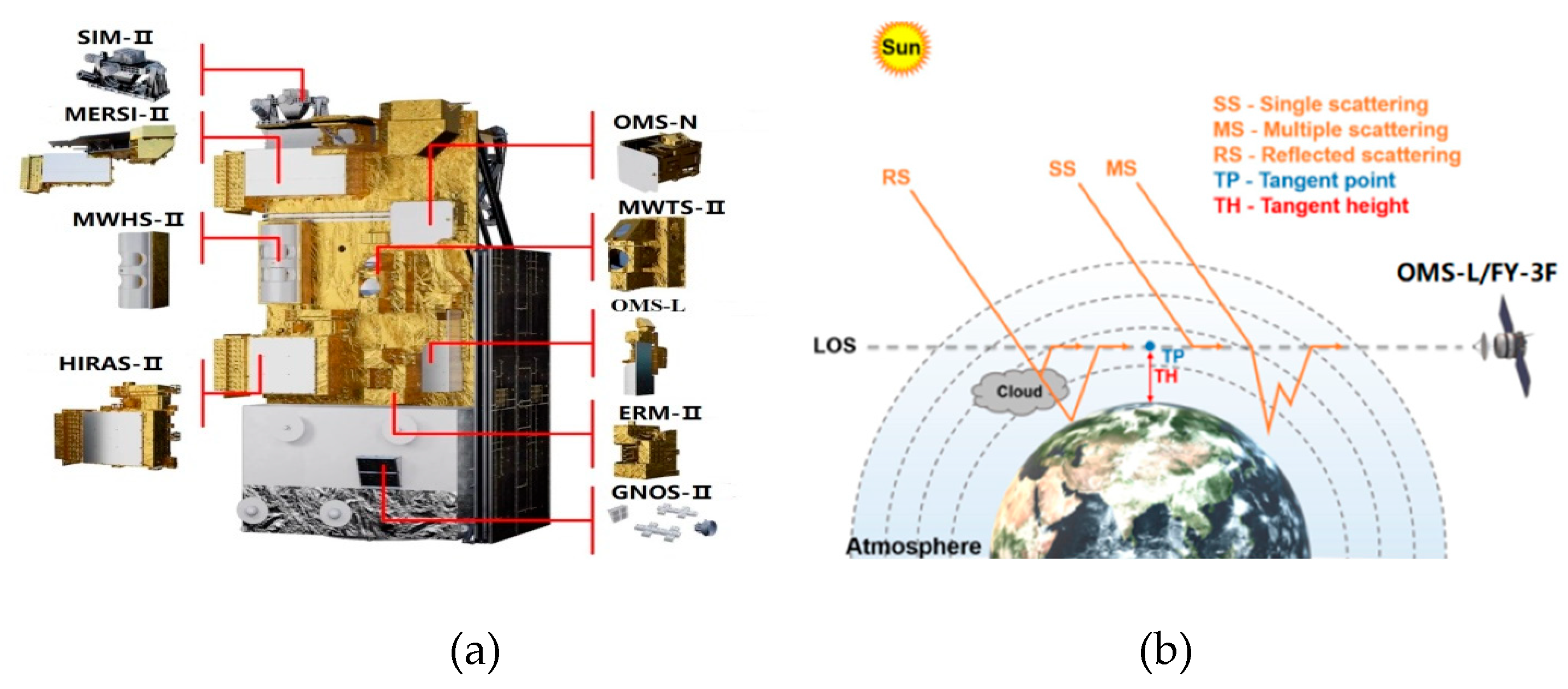
Figure 2.
(a) OMS-L daily orbits and observation geometry sketch, red arrows indicate the satellite flight direction. (b) Sample THs measured by OMS-L during the orbit at 00:47 on the same day. (c) Distribution of limb radiance profiles at a wavelength of 332 nm for different latitudes on the same orbit. (d) Sample set of OMS-L limb radiance profiles for ozone retrieval.
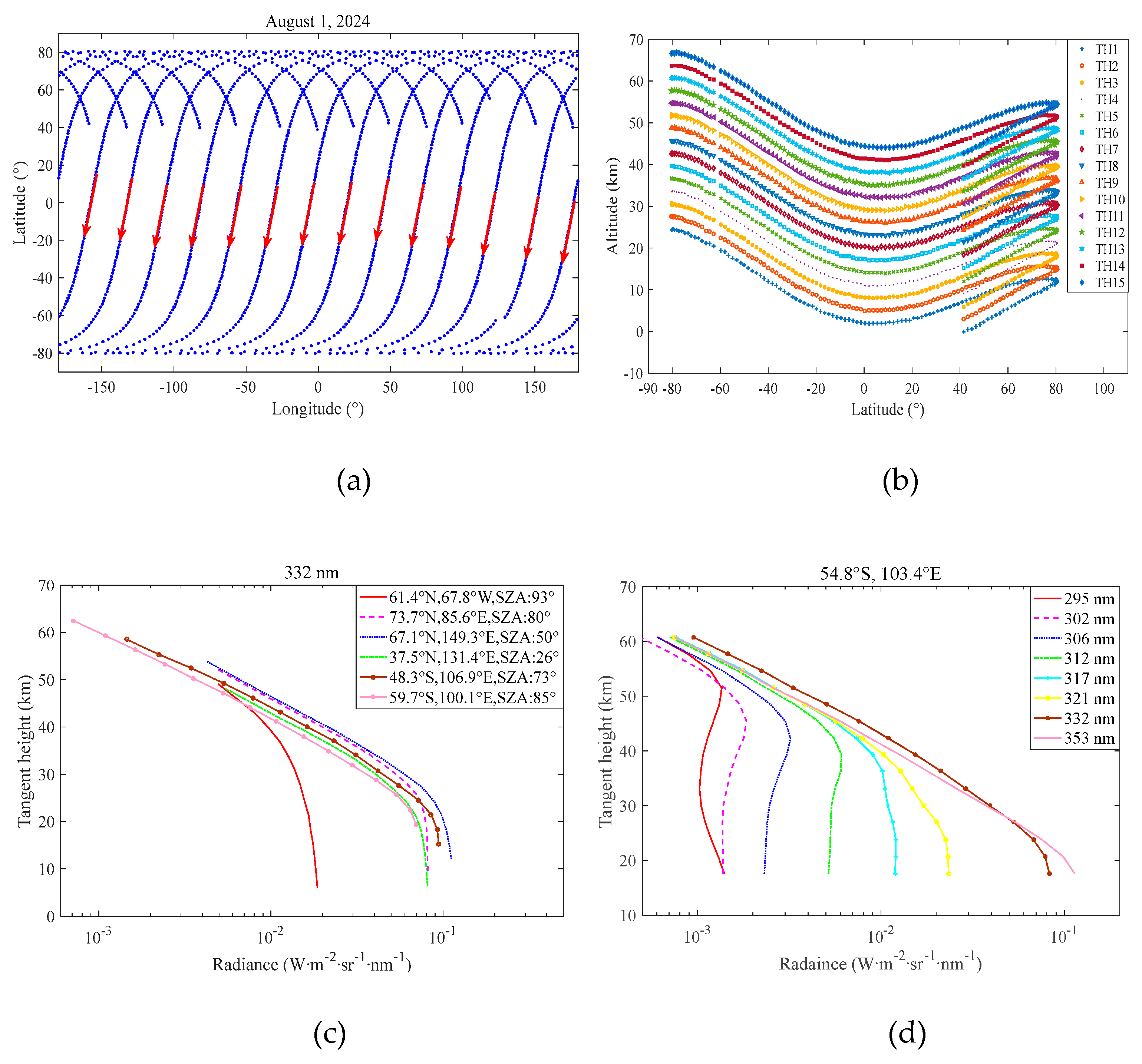
Figure 3.
The sensitivities of the limb radiance calculated by SCIATRAN at selected wavelengths to ozone number density at different altitudes, under the given observation conditions (the SZA is 60°; the relative azimuth angle is 90°). (a) 295nm. (b)302nm. (c) 306nm. (d) 312nm. (e) 317nm. (f) 321nm. (g) 332nm, and (h) 353 nm.
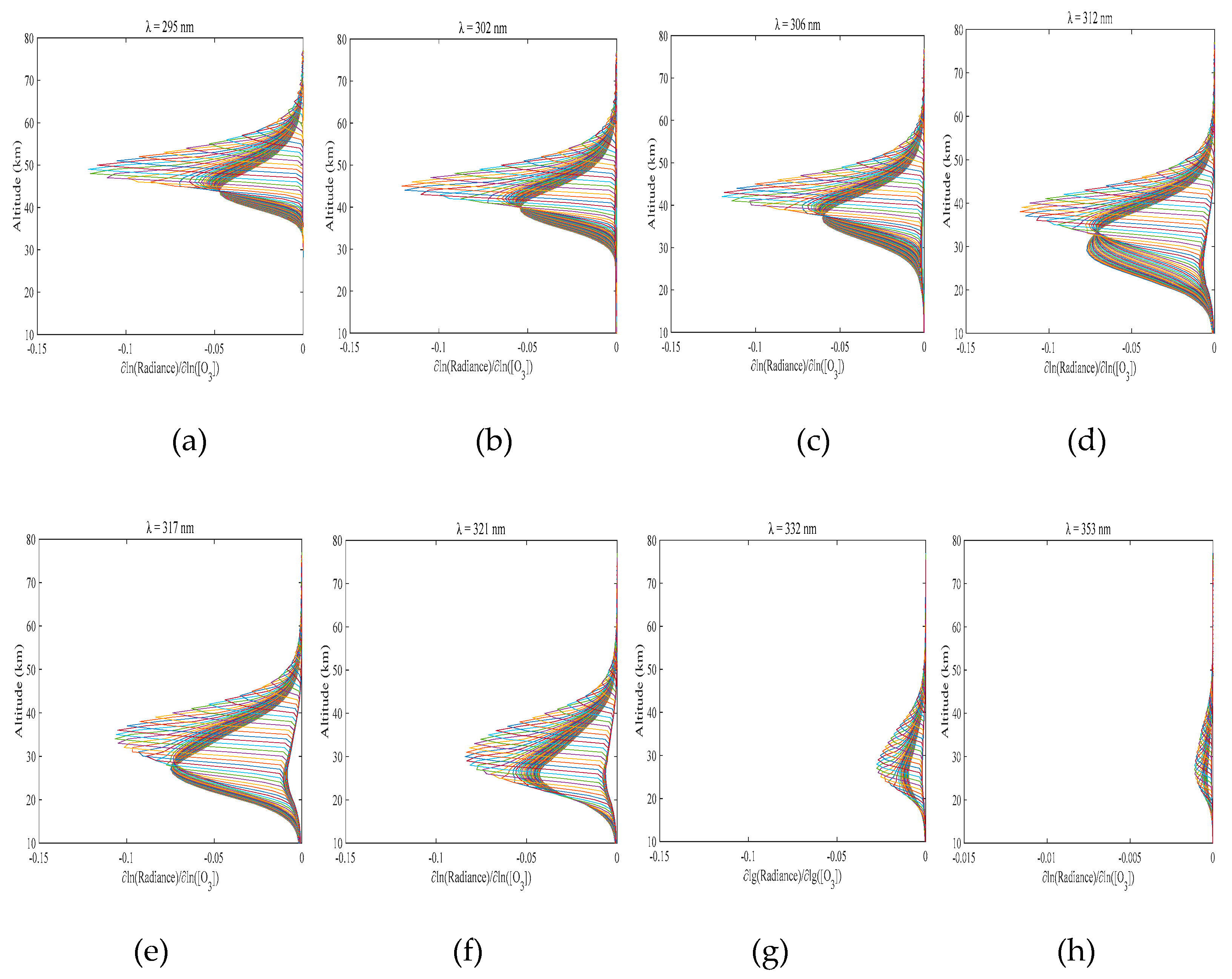
Figure 4.
The wavelength weighting factors assigned to each of vectors as a function of altitude.
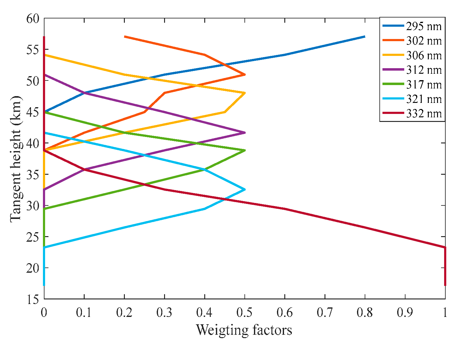
Figure 5.
Ozone retrieval deviations caused by parameter inaccuracies. (a) Different TH offsets. (b) A priori profiles at different latitudes. (c) Different surface albedos. (d) Cloud height of 8-15 km. (e) Aerosol extinction profiles with different scaling factors. (f)Ozone absorption cross-sections with a temperature difference of 20 K. (g) Temperature with an increase and decrease range of ±5 K. (h)Pressure with a scaling factor of ±5%.
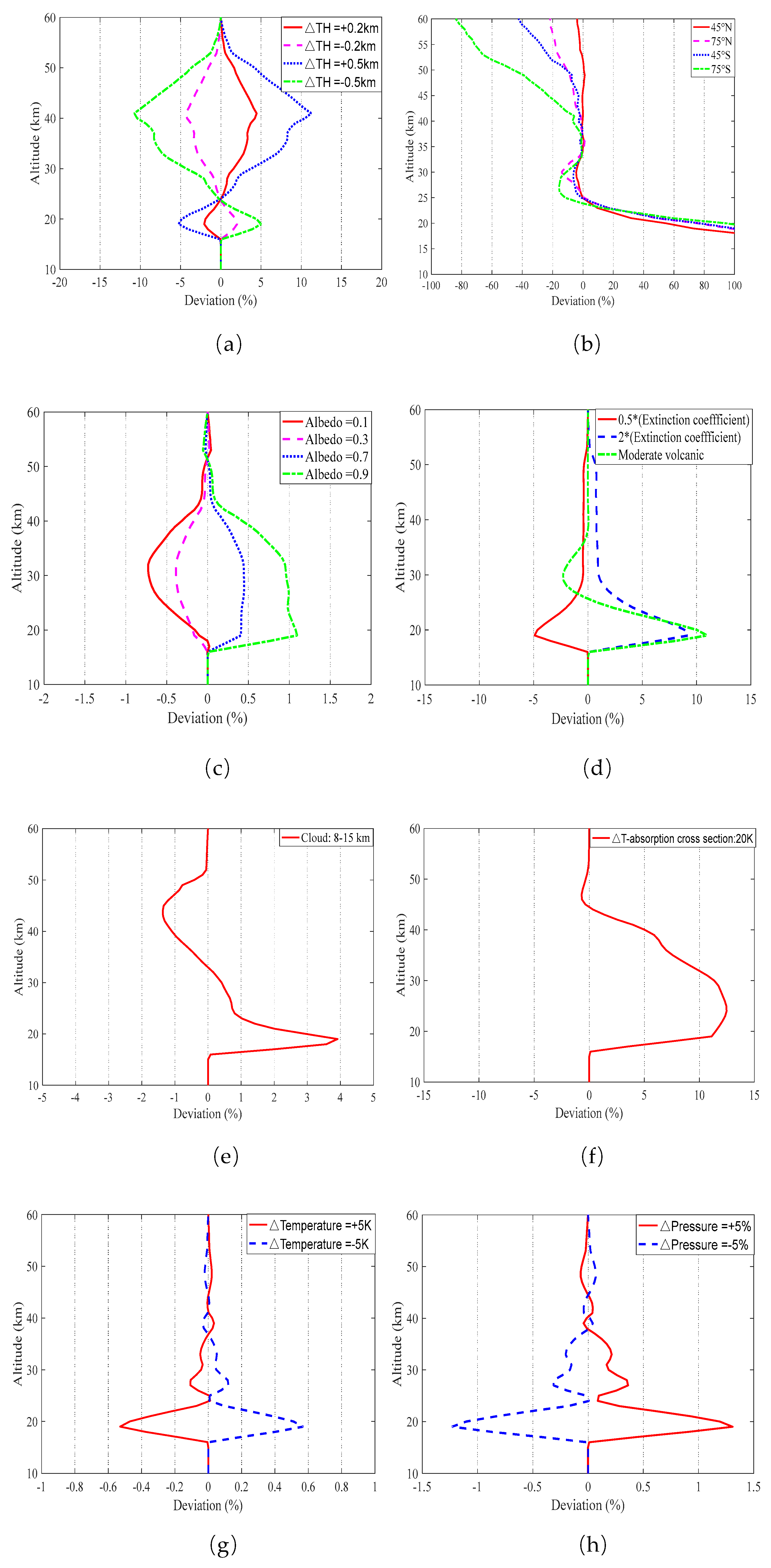
Figure 6.
The estimated profile of the total deviation.
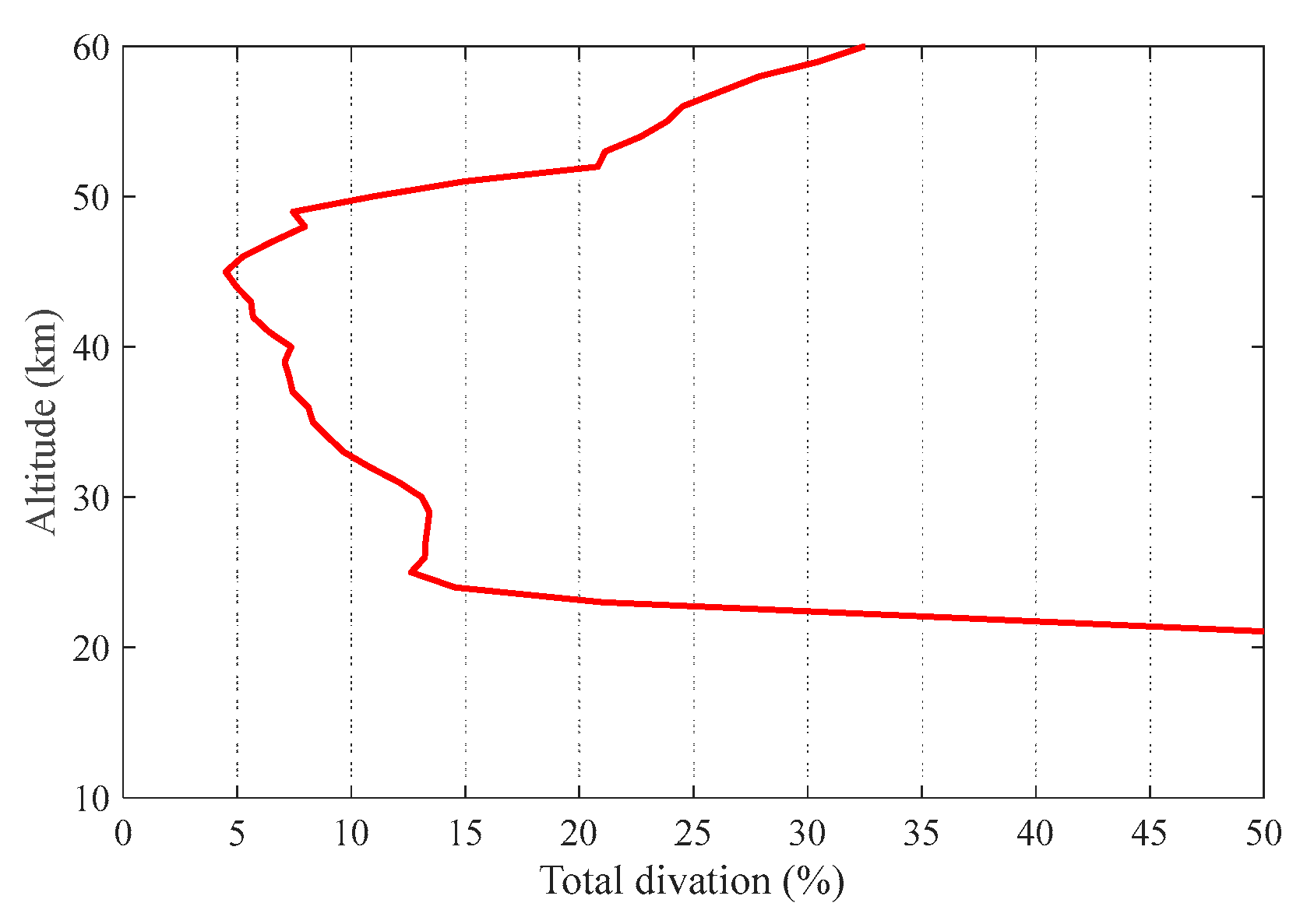
Figure 7.
Observation points of OMS-L and OMPS/LP on the same day. (a) Latitudes and longitudes of all orbits. (b) Matched observation points.
Figure 7.
Observation points of OMS-L and OMPS/LP on the same day. (a) Latitudes and longitudes of all orbits. (b) Matched observation points.
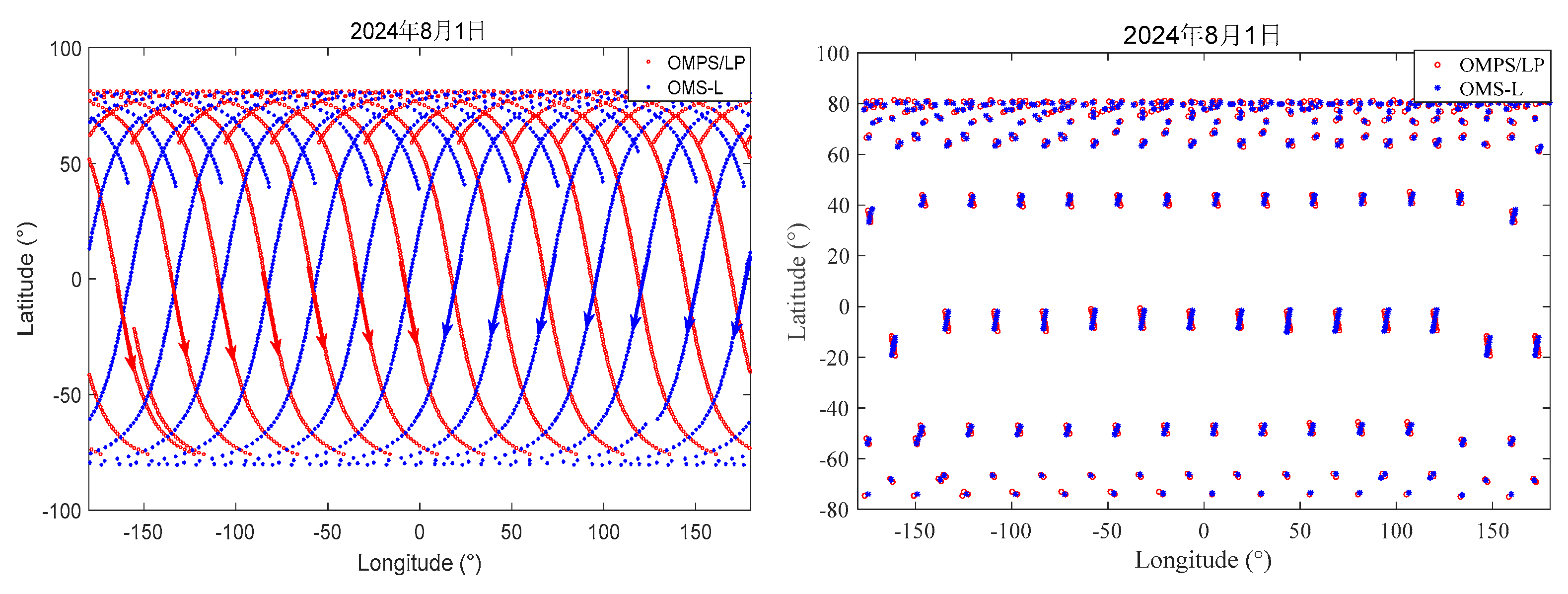
Figure 8.
A selection of single profiles that meet the coincidence criteria at different latitudes, with a comparison between OMS-L and OMPS/LP v2.6.
Figure 8.
A selection of single profiles that meet the coincidence criteria at different latitudes, with a comparison between OMS-L and OMPS/LP v2.6.
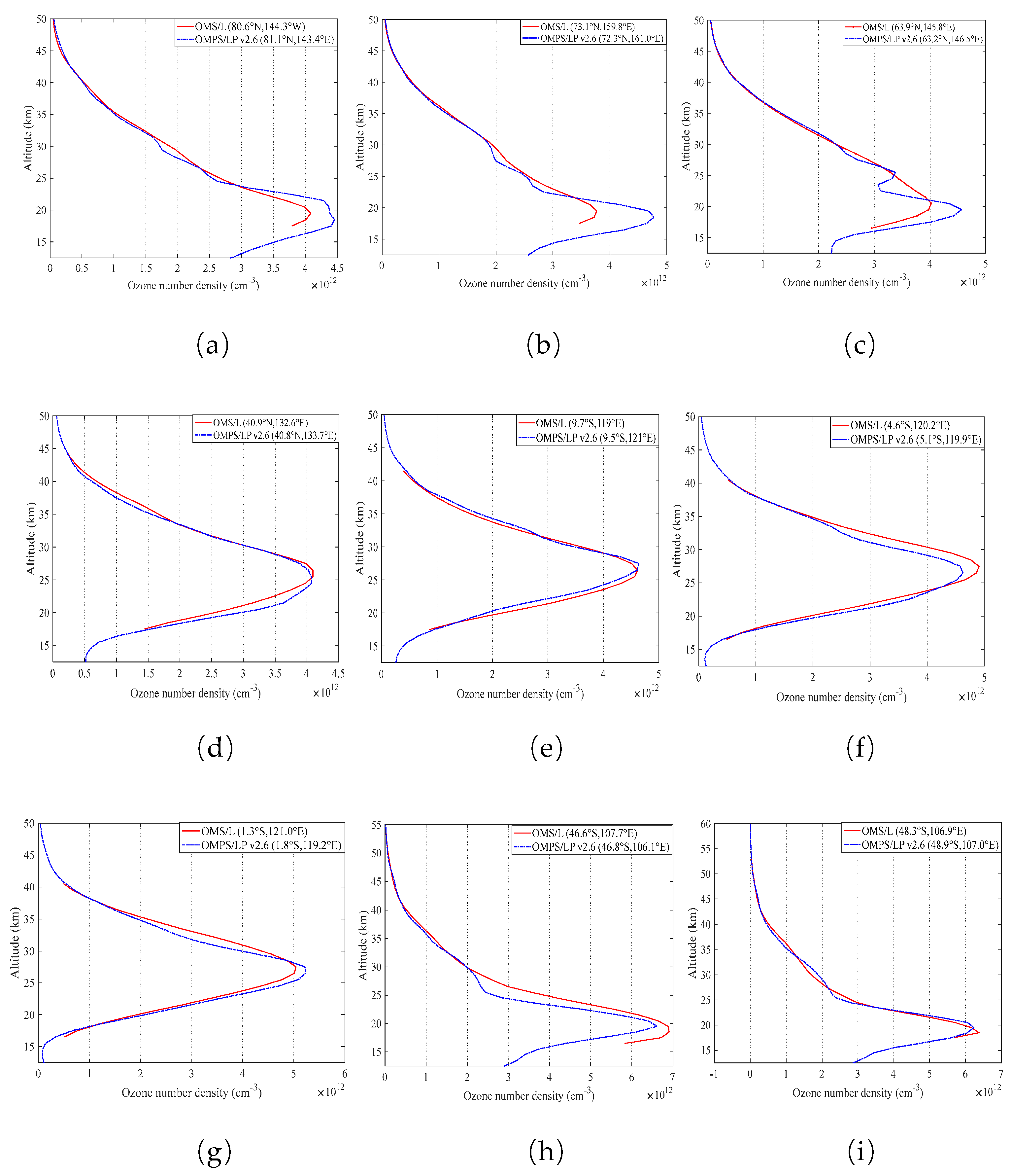
Figure 9.
Comparison of the OMS-L retrievals and OMPS/LP v2.6. (a) Average profile (shaded areas are the standard deviation of the profile). (b) Mean relative difference (dashed line represents standard deviation of difference).
Figure 9.
Comparison of the OMS-L retrievals and OMPS/LP v2.6. (a) Average profile (shaded areas are the standard deviation of the profile). (b) Mean relative difference (dashed line represents standard deviation of difference).
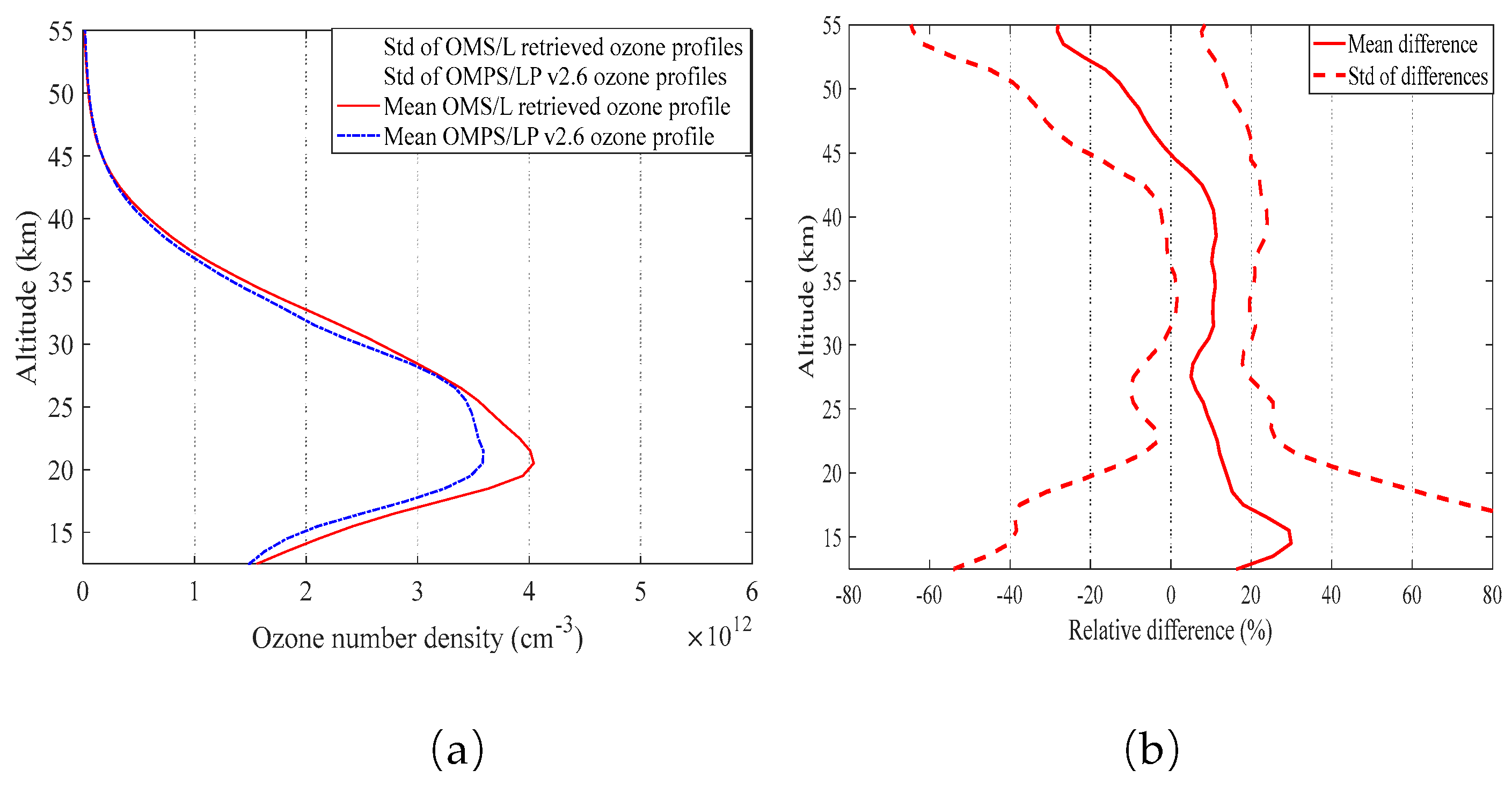
Figure 10.
Comparison of the OMS-L retrievals and OMPS/LP v2.6. (a) Average profile in the northern polar region (shaded areas are the standard deviation of the profile). (b) Mean differences in six latitudinal bands (90°~60°N, 60°~30°N, 30°N~0°, 0°~30°S, 30°~60°S, 60°~90°S).
Figure 10.
Comparison of the OMS-L retrievals and OMPS/LP v2.6. (a) Average profile in the northern polar region (shaded areas are the standard deviation of the profile). (b) Mean differences in six latitudinal bands (90°~60°N, 60°~30°N, 30°N~0°, 0°~30°S, 30°~60°S, 60°~90°S).
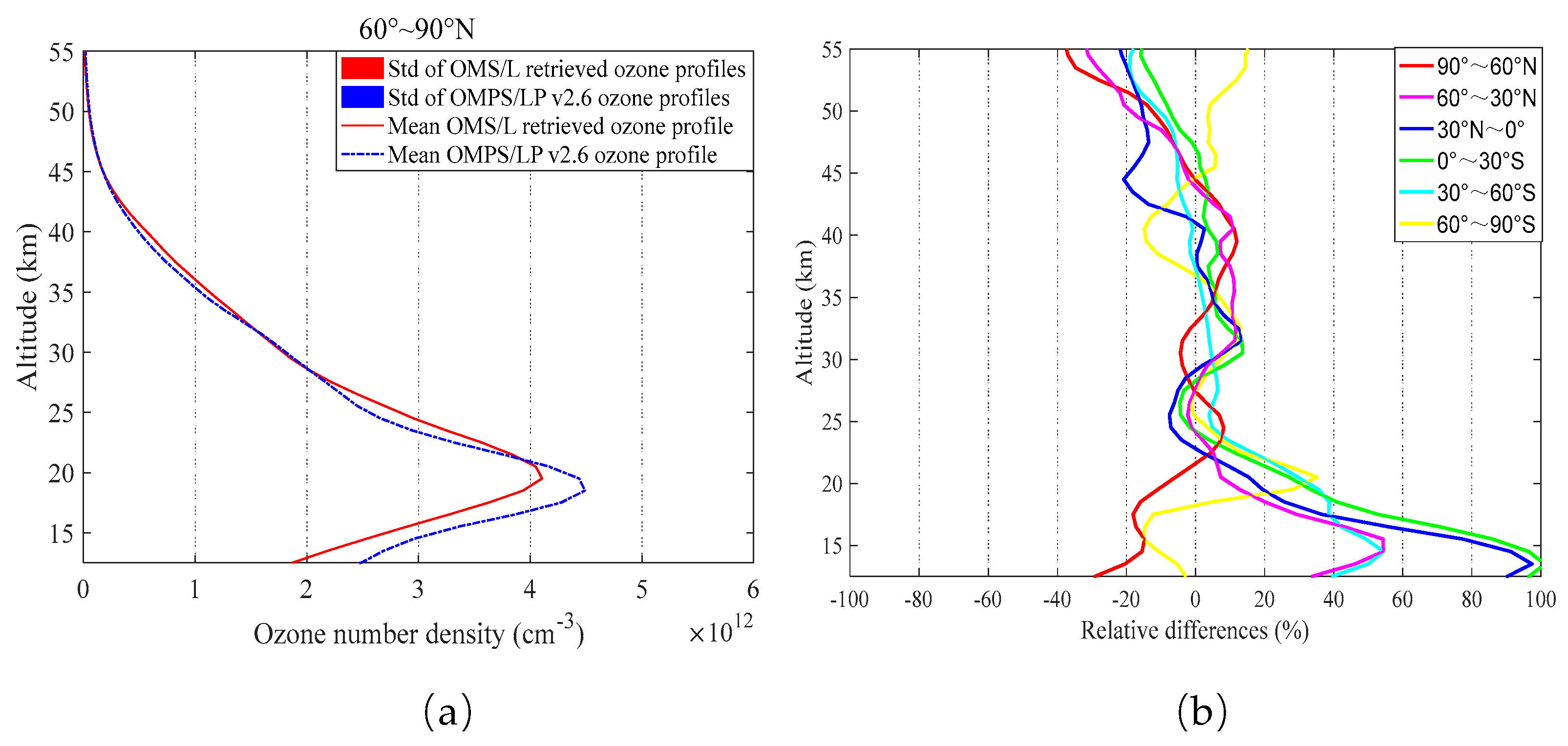

Table 1.
Several main instrument performance indicators of OMS-L [22].
Table 1.
Several main instrument performance indicators of OMS-L [22].
| Item | indicator |
|---|---|
| Spectral coverage | 290-500 nm |
| Spectral resolution | 0.6 nm |
| SNR | >300@0.1μw/(cm2×sr×nm) |
| Vertical coverage | 15-60 km |
| Vertical resolution | 3 km |
| Instantaneous field of view | 2.3°(horizontal)×0.045°(vertical) |
Table 2.
Definitions of the 7 pairs calculated from the measured limb radiances.
| HPV1 | HPV2 | HPV3 | HPV4 | HPV5 | HPV6 | HPV7 | |
|---|---|---|---|---|---|---|---|
| (nm) | 295 | 302 | 306 | 312 | 317 | 321 | 332 |
| (nm) | 353 | 353 | 353 | 353 | 353 | 353 | 353 |
| (km) | 49 | 42 | 42 | 36 | 33 | 27 | 18 |
| (km) | 57 | 54 | 51 | 49 | 42 | 40 | 36 |
| (km) | 60 | 60 | 54 | 52 | 45 | 42 | 40 |
Table 3.
Wavelengths used in the OMPS/LP v2.6 ozone retrieval, according to Kramarova et al. [39].
Table 3.
Wavelengths used in the OMPS/LP v2.6 ozone retrieval, according to Kramarova et al. [39].
| Parameters | Values |
|---|---|
| Wavelength used in UV (nm) | 295, 302, 306, 312, 317, 322 |
| Wavelength used in Vis (nm) | 606 |
| Reference wavelength used in UV (nm) | 353 |
| Reference wavelength used in Vis (nm) | 510,675 |
| Normalization altitude used in UV (km) | 60.5 |
| Normalization altitude used in Vis (km) | 40.5 |
Disclaimer/Publisher’s Note: The statements, opinions and data contained in all publications are solely those of the individual author(s) and contributor(s) and not of MDPI and/or the editor(s). MDPI and/or the editor(s) disclaim responsibility for any injury to people or property resulting from any ideas, methods, instructions or products referred to in the content. |
© 2025 by the authors. Licensee MDPI, Basel, Switzerland. This article is an open access article distributed under the terms and conditions of the Creative Commons Attribution (CC BY) license (http://creativecommons.org/licenses/by/4.0/).
Copyright: This open access article is published under a Creative Commons CC BY 4.0 license, which permit the free download, distribution, and reuse, provided that the author and preprint are cited in any reuse.


