
Submitted:
11 November 2024
Posted:
12 November 2024
You are already at the latest version
Abstract
The operation and modelling of doubly fed induction generators (DFIGs) are quite different in grid-connected and stand-alone operated wind energy conversion systems (WECSs). Researchers usually simulate DFIG in these operations using the pre-built models provided in commercial software which are built using complex modeling techniques that most researchers new in the field are not familiar with. In this paper, a simple and easy-to-use modeling approach based on basic dynamic voltage equations of DFIG is proposed in order to provide a more physical and practical understanding of the dynamic behavior of DFIG. Its fundamental theory and various dynamic models are presented and discussed considering the difference between stand-alone and grid-connected operations. Several effective simulations using the proposed models are performed aiming to have new researchers working in this field to develop a more practical, in-depth and intuitive understanding of the theory and working principle of DFIG in stand-alone and grid connected operations. In addition, uncontrolled and a current-controlled operation of DFIG is realized through simulation and experiment. A small-sized laboratory hardware setup used in the experiment is introduced, and several results obtained for both con-trolled and uncontrolled operation of DFIG are presented.
Keywords:
modelling and simulation of DFIG
; and stand-alone and grid connected operation of WECSs
; variable speed wind turbine system
; vector control of DFIG
1. Introduction
Since there is a global demand for renewable energy that minimizes carbon emissions, wind turbine systems became an attractive research area for the academic and industrial sectors. The current installed modern large-scale, i.e. multi-MW WECSs typically operate at variable speed [1,2]. For these systems, DFIG still stands out as one of the best options for the manufacturing and supplier sectors, due to its important advantages such as requiring small-sized and low-cost power electronic converters and facilitating independent active and reactive power control [3]. Therefore, its market share is expected to continue to increase in the next 5-10 years [4]. However, from a technical standpoint, DFIG is quite interesting and a bit difficult to understand compared to its traditional counterparts such as squirrel-cage induction generator (SGIG), and permanent magnet synchronous generator (PMSG).
In these respect, it is considered that even though the need for engineers employed as maintenance, service and research staff for the industry field is constantly increasing in the world energy sector but most of the new graduated engineers have a serious lack of knowledge about renewable energy conversion systems. Therefore, a particular aim of this study is to fulfill the gap and address the needs of new entrants in this field regarding to the key issues of variable speed turbine systems. Moreover, the paper aims at two points: first, to develop an easy-to-use dynamic model to provide greater physical and practical understanding with effective simulation tests on the basic theory of DFIG; Secondly, to demonstrate how to carry out various tests such as smooth excitation at system startup and to test the working principle of variable speed, constant voltage and constant frequency, stand-alone operation with different types of loads and no-load conditions, connection of DFIG to the grid and intentional islanding, and some other issues from both theoretical and practical perspectives.
From a research and education perspective real experiments of WECS are impractical and applicable less frequently due to lack of access to real systems in the installation sites. Therefore, research and teaching activities regarding WECSs are generally performed on lab scale test setups, but mostly with computer simulation using well-known commercial software packages, such as Matlab/Simulink, Plecs, DigSling, Simpow, and the others. These software packages offer pre-built demo simulation models of physical systems, which are often complex and created with some special toolbox that users might be unfamiliar with [5,6,7,8]. In addition, with regard to these models, it is often difficult to establish the relationship between the mathematical model equations of physical systems and their pre-built simulation models. Thus, these pre-build models are not very effective to understand the underlying relationships and also not appropriate for all real operational requirements in DFIG-based WECSs. Therefore, various modeling approaches have been proposed to meet different research requirements, usually related to large-scale grid-connected variable speed DFIG-WECSs. Moreover, many research and case studies have been proposed to analyze the steady-state and dynamic behavior of the DFIG and furthermore to improve the overall control performance and operational safety, increase the system efficiency and predict and solve the problems under normal and fault conditions. A significant amount of literature on these studies can be found in [3,9,10,11,12,13,14,15,16] and references therein. In these studies, the aerodynamic model of wind turbines has also been extensively investigated. Therefore, to better simplify the system structure and focus on the DFIG machine itself, the above-mentioned extreme points are not considered in this study.
The proposed modeling and simulation approach takes into account the difference between grid-connected and stand-alone operation of DFIG and provides a good opportunity to test both operating modes. It has the advantage that the user can directly build his own model using the building blocks of the appropriate software and optionally take into account the parameter variation of DFIG. In addition, free acceleration testing of DFIM (motoring mode) can be performed using the grid-connected model version to verify its accuracy.
Accordingly, this paper is organized as follows: The basic structure and theoretical background of the DFIG-WEGS are briefly explained with intuitive illustrations in Section II. To clarify the complexity arising from alternative coordinate frames and selectable state variables, the dynamic model equations of DFIG are reviewed. Then, various DFIG models available in the literature are addressed and difference of stand-alone and grid connected DFIG models are discussed in Section III. The structure and building of the proposed simulation model in Matlab/Simulink is presented in Section IV, Section V is devoted to simulation and experimental tests of DFIG. Conclusions are given in Section VI.
2. Operation Principle of DFIG-WEGS
The DFIG is a wound (slip ring) rotor type induction machine, and its construction simply consists of a three-phase stationary winding fixed to the stator and a three-phase rotary winding fixed to the rotor as shown in Figure 1. Since the stator and rotor windings are fed from an ac power source, it is often called a doubly fed induction machine (DFIM) and can therefore be operated in several modes; motor operation, transformer operation and generator operation [9,10,11]. As seen in Figure 1, a prime mover (e.g. diesel engine, wind turbine or other similar unit) is needed to rotate the DFIG rotor shaft for both transformer and generator operations, these are summarized below;
1. In motor operation, the prime mover must be disabled and the rotor windings are short-circuited while the stator winding must be supplied with nominal AC voltage. The adjustment of external resistors connected to the rotor terminals allows the machine to operate at maximum starting torque, as in the old uses of DFIM. In real applications, motor operation is also possible in an alternative way, by supplying nominal AC voltage to the rotor winding and short-circuiting the stator winding.
2. To operate the DFIM as a generator, the prime mover must be enabled to rotate the rotor. In this case, two different operations are possible; operating as a rotating transformer when the rotor (as field winding) is supplied from appropriate ac voltage source, at constant magnitude and frequency, then the stator winding generates an ac voltage at varying frequency and amplitude depending on variation of rotor mechanical angular speed, ωm. If the rotor speed ωm is kept constant, then the stator can generate an ac voltage at constant magnitude and frequency depending on constant slip and slip angle.
The basic structure of a DFIG based WPCS is illustrated in Figure 2, which helps to more physical and intuitive understanding on the working principle of DFIG at variable speed, constant voltage and frequency. In most real applications, the prime mover is replaced by a wind turbine, which coupled to the DFIG's rotor shaft via a gearbox and converts wind power directly into rotary mechanical power via its blades. The turbine shaft speed naturally varies with the wind speed V (m/s) acting at blade slip aria of the turbine at the installation site. So, depending on the rotational speed change, a DFIG can operate in three different modes as listed below [9,10];
- Sub-synchronous mode
- Super-synchronous mode
- Synchronous mode
where, is the synchronous angular speed and fs is the mains or stator voltage constant frequency. As shown in Figure 2, the stator terminal can be directly connected to
the grid (for grid-connected operation) or to external loads (for stand-alone operation) as required.
In real applications, the stator voltage and frequency are adjusted by the rotor flux via controlling the rotor current as the rotor speed changes. This task is normally performed by two power electronic converters connected back to back, as shown in Figure 3. One of these converters works as an active front-end rectifier and is responsible for keeping the DC bus voltage constant, while the other works as a variable frequency PWM voltage source inverter (VSI) responsible for controlling the active and reactive power to be injected from the stator into the grid or an external load by regulating the rotor current [11,12]. However, in order to simplify the structure of simulation system and to understand the working principle of DFIG in the easiest way, the power converters are ignored in this study. Then the variable magnitude and frequency requirement to feed the rotor winding is met with a virtual ac voltage source as shown in Figure 2, which has been created from the stator-rotor voltage relationship given in (1).
where s is normalized slip and θsl is the slip angle, both given in (2), (3) respectively, k is the winding turns ratio (or the rotor-to-stator voltage ratio) if the rotor is at rest, i.e., . In a wind power system, the typical slip range of the DFIG is ±0.3. This means that the slip value can change from +0.3 sub-sync. to -0.3 super-sync at most. The slip angle and its normalized value can be calculated by (2) and (3), respectively [9,10].
Here, it should be noted that if the DFIG’s rotor is stay at stand-still, i.e., , , and slip s=1, then both rotor and stator voltage frequency will be same, i.e. fr = fs. In this case, the rotor voltage magnitude is determined only by the winding turn ratio, k. Thus, the voltage relationship given in (1) becomes at , and in this particular case a DFIG works like a transformer, which is unsuitable operation for the power production purpose. But, if the rotor is rotating at any speed, the voltage equation given in (1) is always valid and the relationship between the rotor-stator frequency is fr = s.fs, and the relationship between active powers is Pr = s.Ps. Therefore, it can be clearly seen that a DFIG allows bi-directional power flow through the rotor as the direction of the rotor current is reversed depending on whether the rotor speed is higher or lower than the synchronous speed. It can be understood that both stator and rotor can supply power to the grid in super-synchronous operation. To achieve this, a set of back-to-back power converters are needed to regulate the DFIG rotor current. In this context, there are several considerations that should be taken into account for a DFIG based WECS [13,14];
1. Initial excitation; The rotor has to be fed with adjustable ac current to create a magnetic field in air gap of the machine and induce generator voltage on the stator. The supply voltage can be obtained from utility grid for the grid connected operation. But for the stand-alone operation at the ruler area, there are several methods to fix this problem without requiring an external power supply as described in Figure 3. One way is to use an energy-storage (small battery or super-capacitor) element with isolating diode in the DC link and the second way is to use the residual magnet in the core of the machine and with additional AC capacitor at the stator terminal, another solution can be fitted with a pilot generator on the rotor shaft feeding the excitation winding [11].
2. Power imbalance; The power imbalance: The power delivered to grid is determined by the MPPT mechanism depending on wind speed at the wind farm for the grid connected operation, its limited with the generator rated power. But the imbalance between the captured wind power and the demanded power of the external load is one of the main challenges for stand-alone wind turbine systems. If the mechanical power received from the wind is greater than the power consumed by the load, then pitch angle controller is activated to adjust the pitch angle to ensure that the rotor speed is inside the allowable operating range. In the opposite case that the captured wind power is not sufficient for the connected load. The wind turbine tries compensating the power shortage by the energy stored in its inertia and supplying the load during a certain period of time or preventing excessive decrease of rotor speed with an appropriate load shedding. This must be considered in order to guarantee the system against total collapse and to cater a secure power supply to high priority loads. More detailed information about the design criteria, and requirements to start up and run the system, as well as the economic advantages of the DFIG based stand-alone WEGS can be found in [2,3,9,10].
3. Various Model of DFIG
As mentioned above, if the rotor windings are short-circuited, a DFIM can be considered to have the same structure and the same dynamic model as a three-phase squirrel-cage induction machine (SGIM). For the simplicity, it should be noted that the dynamic model equations of IMs are derived under several assumptions [16]; The three-phase windings are star-connected, symmetrically balanced, and have sinusoidal distribution, the magnetic core of the machine is linear, magnetic saturation, skin effects of wires, and the iron losses are neglected. Under these assumptions, a general model as a compact set of nonlinear differential equations derived from the electromagnetic relationship between the stator and rotor windings will be used to describe the dynamics of both IMs (SGIM/DFIM). However, the equations of the three-phase IM model are usually complex because the state variables and inductances of each phase winding of the stator and rotor varies sinusoidally and are cross-coupled with each other. Therefore, based on the space vector theory, an equivalent space vector model equation defined on two orthogonal axes is preferred to represent a three-phase IM. Because the space vector theory simplifies the mathematical model of the IM, since it allows the transformation of the three-phase instantaneous state equations into equivalent two-phase space vector equations and eliminates the complexity of time-varying inductances. The derivation of an equivalent two-phase model of IMs and the formulation of phase and coordinate transformations using the well-known Clark and Park transformations can be found in detail in [16,17]. Accordingly, each of the three-phase sinusoidal variables (i.e. voltages, currents and flux linkages) can be represented by a space vector and in this context, the space vector equivalent circuit of a DFIM can be introduced as shown in Figure 4.
From Figure 4, the basic dynamic model equations of a DFIG can be derived based on the space voltage vector of the stator and rotor given in (4) and (5), which are defined on the natural (separated) frame axis (sr-axis) and valid for both SGIM/DFIM.
where it is assumed that the rotor parameters are reduced to the stator, and flux linkages are defined as follows:
where
: stator and rotor voltage space vectors (V)
: stator and rotor flux space vectors (Wb)
: stator and rotor current space vectors (A)
Ls, Lr : stator and rotor inductances (H)
Rs, Rr : stator and rotor winding resistances (Ω)
: rotating synchronous speed (rad/s)
: rotor electrical angular speed (rad/s)
: angle between stator and rotor winding axes
where superscripts “s” and “r” denote the variables are referred to respective reference frames with s is the stationary frame fixed to the stator axis and r is the rotating frame fixed the rotor, respectively. The indices s and r indicates the stator and rotor variables, respectively. The is called as rotary unit vector (i.e. shift operator) used for the coordinate transformation between the reference coordinate frames, and is angle between the stator and rotor winding axes. Each of the stator and rotor electrical variables, i.e. voltage, current and flux linkage, presented as complex space vector, can be decomposed into real and imaginary parts in the respective reference frame: i.e. for the stator variables and for the rotor variables .
Remark: Some authors oppose the complex representation of space vectors, i.e. and insist that they should be represented by two orthogonal components such as [18]. However, it is well-known that if representation of is used for the orthogonal space vector model and is used for the complex space vector model, both symbolic notations yield the same dynamic model. Therefore, it does not matter which notation is used to represent the model.
Considering above assumption, two version of the stator voltage space vector equation (4) can be rewritten with help of and (6);
Both equations above consist of two parts; the internal voltage drop, and emf, which is induced by the rotor flux [1]. Using equation (8) a simplified equivalent circuit and phasor diagram of DFIG stator can be drawn similar to that of a synchronous generator as shown in Figure 5. Under the no-load operation, the stator current and hence the internal voltage drop is zero and thus the stator terminal voltage becomes equal to the induced stator voltage, i.e. , which is given as the function of rotor current and mutual inductance by
For the full-state model of a DFIG/M, its mechanical part must also be taken into account, which is given in (10)
where, is the mechanical torque acting on the rotor shaft which can be an external mechanical load in case of motor mode operation, or it can be an input provided by a wind turbine in case of generation mode in WEGS, ɷm is the rotor mechanical angular speed, p is pole pair of the machine, is the electromagnetic torque produced in the air gap of the machine that can be defined in several alternative ways; i.e. it can be defined as function of space vectors of the stator current and rotor flux i.e. where (*) denotes the complex conjugate), the other torque expressions with different state variables are explained well in [15]. It should be noted here that the angular velocity or mechanical torque transmitted from the wind turbine to the DFIM rotor shaft can be considered as optional input to the system’s mechanical part when it is operating in generator mode.
The separated frame model equations in (4)-(6) can be redefined by considering different state variables and alternative reference frame axes. To achieve this, the stator and rotor voltage space vectors given in (4), (5) are multiplied by the phase shift operator depending on the selected reference frame angle. For example, if the voltage equation (4) is multiplied by then it will be represented in the rotor frame (DQ-axis), and if (5) is multiplied by it will be presented in the stationary frame (αβ-axis). Similarly, it is also possible to represent the same equations (4) and (5) on an arbitrarily chosen general rotating reference frame (xy-axis). For this end, the stator voltage space vector is multiplied by and the rotor voltage space vector is multiplied by . Here is angle between the stationary frame (αβ-axis) and an arbitrary chosen common rotating reference frame (xy-axis). The above multiplication results in the derivation of the general frame model equations defined on the xy-axis.
where subscript “g” briefly denotes xy-axis and the relationship between the flux and current variables are given as
Depending on the specific analysis intended or targeted, the model equations (11) and (12) can be redefined with the aid of (13) and expressed for optional state variables; i.e. the stator and rotor currents stator and rotor fluxes stator current and rotor flux or stator flux and rotor current For example, a model with the flux state variables can be called as “flux model” and obtained as:
This is the simplest model of IM/DFIM and can be defined for alternative state variables using equation (13) and i.e. if (14) and (15) are rearranged for the stator and rotor currents space vector, it might be called as “current model” and is derived as:
Considering the orthogonal components of the state variables, both the flux model and current model can be expressed in state-space form. For example, from equations (16) and (17), the state-space current model defined on the xy-axis can be obtained as given in (18), where both stator and rotor voltages, and the external mechanical torque tL (or optionally the rotor mechanical angular speed, are considered as the inputs of the DFIG system. Here it can be seen that rotor electrical speed is one of the state variables of the system and it exits in the system matrix A. This is the main reason why DFIM is a non-linear system [9].
The flux model equations (14), (15) with (10) and the current model (16), (17) with (10) both can represent the well-known 5th-order nonlinear model equations of an induction machine. These models are valid for both the SGIM and DFIM/DFIG. A version of these models defined in dq-axis are generally used in many research studies to simulate the controlled operation of grid connected DFIG with back-to-back converters under different operation conditions. In these applications, active and reactive power are injected into the grid by regulating the rotor current through a pulse width modulated voltage source inverter (PWM-VSI) with power and current feedback control depending on the input references determined by external (active and reactive power) controllers. In this case, an MPPT controller generates an active power reference based on wind speed, while the reactive power reference is determined by the power quality demands. Regarding the grid connected operation of DFIG, there are many research studies to solve different operational problems and application of different control strategies such as direct torque and direct power control under normal and abnormal operating conditions, and even more, there are various research studies focusing on different existing problems, so these latter issues are ignored in this paper. However, a basic simulation test on the control of rotor current is presented in the following section.
On the other hand, it has been reported about 5th order models (flux and current based models with the mechanical equation) that they lead to a complex system structure and are not suitable for analysis studies in operations under transient conditions for large-scale wind energy applications, so it is necessary to develop a simplified DFIG model to study on such systems, an example of simplified model presented in [19]. Different approaches proposed for the simplified DFIG model, aimed at shortening the computation time and simulating large-scale wind power applications, and analyzing challenging problems occurring in transient, normal and abnormal operations can be found in [20,21,22,23].
3.1. Various Coordinate Frame Models
As mentioned earlier, there are several alternative model equations defined in various coordinate frames shown in Figure 5. and can be obtained from (18) by appropriate coordinate transformations. An easy way to obtain these models defined in various reference frames is to replace the angular velocity ɷg in the model equations [16,17] with any of the ones listed below.
ɷg = ɷg for the arbitrary selected rotating frame (xy-axis)
ɷg= ɷs for the synchronously rotating frame (dq-axis)
ɷg = ɷr for the rotating frame fixed to rotor (DQ-axis)
ɷg = 0 for the stationery frame fixed to stator (αβ-axis)
However, it is often common for new learners to be confused in understanding and distinguishing between these various models, so an easy and accurate explanation of the relationship between these models can clarify the contradiction. For example, if the arbitrary selected angular speed is taken as ɷg=0 in (11) and ɷg=ɷr in (12), this general frame model equations (11), (12) will return to the same with the separate frame model equations in (4) and (5). Another example, if we take ɷg=0 in (11) and (12) or alternatively in the rows of (18), the general frame model will be transformed into the stationery frame (αβ-axis) model. Similarly, it is possible to derive a model defined in any frame axis from equations of the general reference frame model in (11), (12).
Figure 6.
Coordinate frames of DFIG/DFIM.
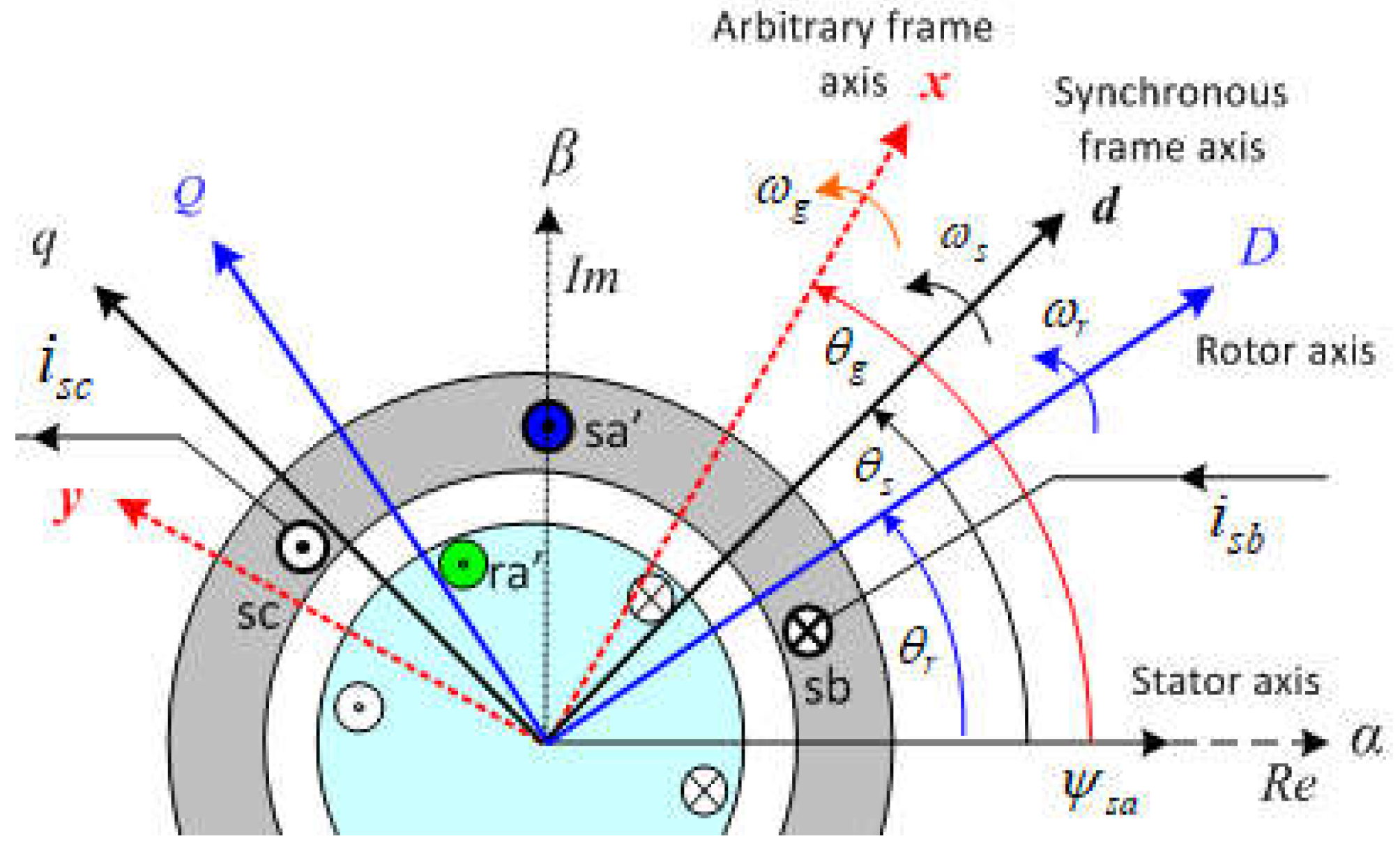
For example, replacing ɷs with ɷg in (11) and (12) will transform the general frame model into another model defined in the synchronously rotating frame (dq-axis), or replacing ɷs with ɷr will transform the same model into another model defined in the rotating frame with rotor (DQ-axis). However, what is important here is that the voltages supplied to the stator and rotor are compatible with the reference frame in which the model is defined and that the appropriate coordinate transformation must be done for the other state variables.
3.1.1. Grid Connected Model
As mentioned above, the stator and rotor voltages are defined as (double voltage) inputs in the flux and current based models which are appropriate for the analysis of grid connected DFIG operation and hence these models can be called as “grid connected model” of DFIG. For the proposed grid-connected simulation model of DFIG, the flux model given in (13) and (14) is used, which can be rewritten with its orthogonal components as:
In the simulation, instead of the flux-based model given above, the current-based model in (18) can also be used as an alternative option.
3.1.2. Steady-State Model
Flux and current models can also be used for the analysis and simulation of the steady-state behavior of the DFIG when the derivative of the state variables is equal to zero. In this context, many comprehensive studies on steady-state analysis for DFIG-WEGS have been conducted in the literature [9,10,20] so this topic is not the focus of this study.
3.1.3. Motor Model (DFIM)
As it is stated before a DFIG can be run as an IM. It should be noted here that both flux and current models can also be used to simulate motor operation of a DFIM by short-circuiting one of the winding ends of the stator or rotor and then applying an AC voltage to the other winding as is done in real applications. This can be easily accomplished in simulation, for example, by applying zero volts (or short-circuiting) to the rotor terminals and then applying nominal voltage or less to the stator.
3.2. Stand-Alone Models
The current model in (18) and the flux model in (19) and (20) are not suitable for simulation a stand-alone operated DFIG since they both take the stator and rotor voltages as inputs to the system. Therefore, this paper particularly focuses on deriving a simple simulation model needed for stand-alone DFIG which provides us a better grasping of the fundamentals of DFIG and also facilitates the analysis of its dynamic behavior under different conditions. It should be noted here that the difference between a stand-alone and grid-connected model is that the stator voltage in a grid-connected DFIG is supplied from the grid, but a stand-alone DFIG generates voltage at the stator terminal as its output and supplies to external loads connected to the stator terminal.
Thus, the equation (18) can be extended and adapted for the stand-alone model based on some reasonable assumptions [Abad]. First, it is assumed that only a resistive load is connected to the stator, and secondly, in addition to resistive load, the stator terminal is also equipped with a filtering capacitor. However, with only the external resistive load R0, the stator voltage will be the same as the voltage drop across the external load connected to the stator, resulting in
where the stator current is the same as the load current, Replacing the stator voltage in (18) with the auxiliary equation in (21), a stand-alone DFIG model can be derived in the state space form [9,10,11]:
where the stator and rotor current components are state variables, the stator voltage is eliminated and the rotor voltage become only the input of the system. The stator current also can be considered as the disturbance of the system. Considering here that the stator voltage and current are linearly dependent for resistive loads, equation (18) can be further expanded and a different model can be obtained having the stator voltage and rotor current as state variables.
Alternatively, with the second assumption given above, since the stator is connected to resistive load and also has a filtering capacitor Cf, an additional equation for the stator voltage can be obtained as follows:
where indicates resistive load current. With the help of (22) the stator voltage, which is identical with capacitor voltage () can be presented as one of the state variables in the system and an alternative state-space model of the stand-alone DFIG can be obtained as given in (25). More details about models of (22), (23) and (25) can be found in [9,11].
Discussion: It can be said that pure resistive load application is unrealistic and rarely realized in a stand-alone DFIG-WEGS, it is insufficient to analyze the behavior of DFIG in case of different load type and size, and also the resistive load and filtering capacitor complicate the system model.
Considering a stand-alone DFIG, the stator terminal voltage is the same as the load voltage and will vary depending on the load current. Therefore, including the dynamics of various sizes and types of loads makes the dynamic model of the system more complicated, thus making it difficult to obtain a generalized model. Based on this difficulty, a more realistic modeling approach is needed for the analysis of stand-alone DFIG under various operating conditions.
4. Proposed Modeling Approach and Simulations
4.1. Proposed DFIG Models
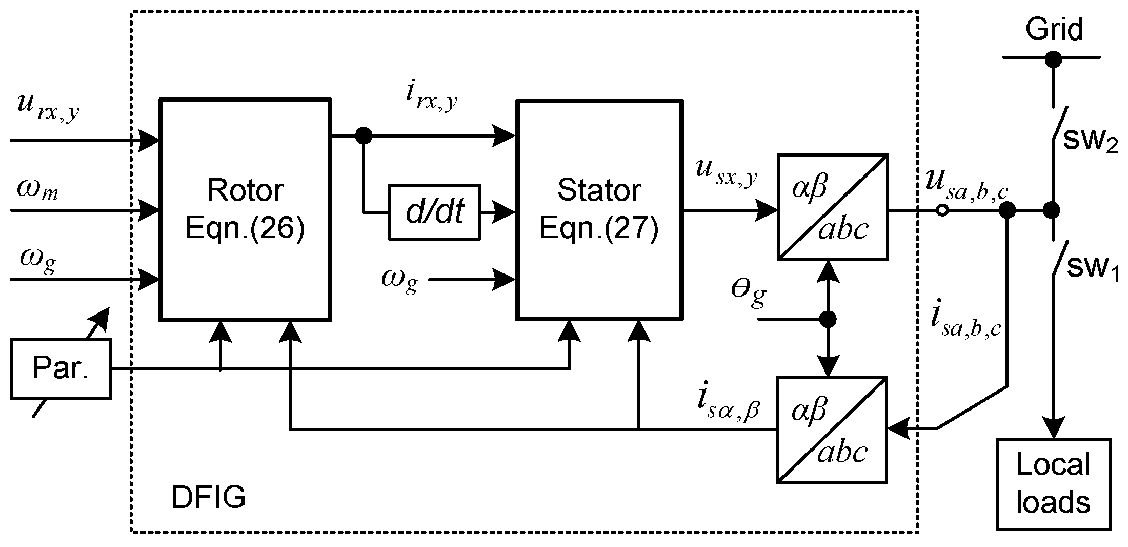
In this study, two simple dynamic simulation models of DFIG are considered; one for the grid connected operation the flux model equations in (19) and (20) are used. But for the stand-alone model a reasonable assumption is made; the rotor side is the primary, the rotor voltage is the input, the stator side is the secondary and the stator voltage is the output of the DFIG system, as is occurred in real applications of stand-alone DFIG. Based on this fact a small modification is made to the current and flux models to allow these models to be used in the simulation of the stand-alone DFIG. In accordance with real applications the stator terminal is open circuited and the dynamics of various size and types of un-modeled loads will be introduced into the system by activating the loads directly by switching. Accordingly, the behavior of DFIG with respect to different load conditions including transient will be simulated and analyzed.
As stated above, if the rotor voltage and mechanical angular speed are considered as the inputs of the system. In this case, the rotor side can be represented by the rotor current dynamic equation in the proposed stand-alone DFIG model which can be derived either from (20) with (13) or directly from the orthogonal components of (17) in xy-axis:
where . It is obvious that connecting different size and type of external loads to the stator results in a different internal voltage drop across the stator winding in real applications. Based on this fact we assume that un-modeled load dynamics can be introduced into the system when an external load is connected to the stator. Therefore, in this study, we consider the stator voltage as the output variable of the DFIG system, which can be derived either from (19) or from (16) as its orthogonal components on the xy-axis:
where it is clear that the stator voltage is determined by the load current through the stator winding and the rotor current regulated by a controller. By using equations (26) and (27), a complete signal flow diagram of the proposed stand-alone DFIG model can be constructed in which the stator current is fed back into the model equations of the stator and rotor when an external load is connected, as shown in Figure. 6. This way resembles real applications and can solve the difficult problem of finding a suitable mathematical dynamic equation of the stator for stand-alone operated DFIG with different types and sizes of external loads. It should be noted here that the flux-based model in (18), (19) can be used in the same way as the current model in (26) and (27), but in this case it is necessary to convert the flux to current using equation (13).
Figure 6.
Signal flow diagram of proposed stand-alone DFIG model in xy-axis frame.
Remark: A minor problem with the proposed stand-alone simulation model in (26), (27) is that during the activation of external loads, a rapid change in transient load current causes unbounded spike in the stator voltage. This is because the total inductance in the stator current path is insufficient to slow down the rapid change of transient current, creating difficulty in numerically calculating the time derivative of the rapidly changing stator current. Therefore, given the availability of line and generator inductance in real application of DFIG, an external line inductor can be inserted into the stator current path. Therefore, in the simulation model, it is acceptable to pass the load current through an additional line filter before calculating the derivative of the stator current, even if this causes a minor change in the system structure.
The proposed simulation models of DFIG are built (19), (20) and the other for standalone operation using equations (26) and (27). Both simulation models are built in Matlab/Simulink using the building blocks, one for grid-connected operation using equations Both simulation models are built in Matlab/Simulink and stand-alone building blocks are used to build them. But, in the standalone model the specialized blocks in Simulink/Simscape tools are used for the external loads, the power supply of the grid, and the switching and measuring devices. In addition, transition blocks are required to pass the signals from Simulink standard blocks to Simscape blocks. It is possible to extend these model for different research requirements, for example, adding harmonic filters and crowbar resistors, etc. An overview of both proposed Simulation models of DFIG are shown in Figure 7. and Figure 8, respectively. Simulation models of DFIG are shown in Figure 7. and Figure 8., respectively.
The proposed modelling approach is more similar to a real stand-alone DFIG system in that it provides flexibility with the advantage of being able to change the types and sizes of external loads. In addition, once the model is created on the general frame xy-axis, it can be easily transformed to any reference frame model of the user's choice by replacing ɷg with one of ɷs, ɷr, and 0 as needed. However, the variables of the system (currents, voltages and orientation angle) must be adapted to each selected reference frame. Another advantage of the model is that it allows the use of nominal values or deliberately distorted values of machine parameters. This can be easily done by passing each parameter through timed step blocks in the Simulink model, allowing parameter variation within a given simulation time. Thus, the proposed DFIG model can be processed to analyze many different scenarios, occurring in WECSs similar to real applications.
A different version of the proposed DFIG model defined on the separate frame axes and two different pre-built models provided in Plecs and Simulink/Simscape were comparatively simulated in a previous study [24], verifying the effectiveness of the proposed modeling approach.
4.2. Simulations
The proposed grid connected and standalone models of DFIG have been simulated for different purposes using the parameters listed in Table 1, [25].
4.2.1. Grid Connected Model Tests
The simulation tests are performed using the flux model for two different purposes: motor running test for DFIM and grid connected operation of DFIG with closed-loop current control.
- Motor operation;
As mentioned before, a DFIG can operate as a squirrel cage IM (SCIM). To verify this fact, first the simulation of the DFIM is performed for free acceleration, which proves the accuracy of the model if it reproduces the well-known typical properties of a SCIM. Here, the stationary frame (αβ-axis) model is used by setting ɷg to zero, which transforms the general frame model into the stationary frame. The stator is supplied with its nominal voltage (in αβ-axis) and rotor voltage is set to zero volts (i.e. the rotor is short-circuited).
Some of the results obtained from the simulation test are shown in Figure 9, where the graphs are the stator and rotor fluxes, stator and rotor currents, electromagnetic torque and angular velocity from top to bottom, exhibiting the typical transient behavior of an IM and verifying the accuracy of the simulation model used. The same result can be obtained from the transformed current model in αβ-axis given in (18).
- 2.
- Grid connected generator operation;
This simulation test is done to show how the stator voltage is regulated by controlling the rotor current, as an example of its controlled operation. At the start, the stator is already directly connected to the grid (to eliminate the need for synchronization) and also the rotor is rotated below the synchronous speed ωr = 35.π (= 110) rad/sec and the rotor current components references have not yet been applied. Therefore, at start time there is no rotor current, but the stator receives a strong current from grid with large transient oscillations. Interestingly, the rotor phase voltages are uniform and have the same frequency as the stator voltage. Also, the stator voltage has the same frequency and magnitude as the grid voltage because the stator is already connected to the grid and is well synchronized. When the rotor q-axis current reference is set to zero (irq*=0) and a stepped d-axis current reference is applied to the controller input at 0.2 seconds, the magnitude of rotor phase currents increases step by step, similar to ird*. At the 1st second the rotor speed is increased to ωr = 45.π (= 141) rad/sec, during this speed change the rotor phase voltages decrease to almost half magnitude, but the rotor currents are unaffected. At 1.5 seconds the rotor d-axis reference current ird* is applied in a sudden step (from zero to 4A) which increases the stator and rotor phase currents. At 2nd seconds the rotor speed is increased once again to ωr = 55.π (= 172) rad/sec (above the synchronous speed), during which the rotor phase voltages change direction but remain constant in magnitude (because the slip remains the same at the previous speed), all above events are shown in Figure 10.
4.2.2. Stand-Alone Model Test
The simulation model of stand-alone operated DFIG is built accordingly signal flow diagram shown in Figure 6, and tested using the same parameter in Table. I. The simulations are performed on the αβ-axis by seting ɷg=0 in (26), (27). The rotor voltage required for a smooth start to generate the stator voltage is obtained through (1), where a reference stator voltage is used that increases from zero to its nominal value and the rotor speed is started at a constant value (30% of the nominal value) below the synchronous speed. Then, a sequential and timed operation strategy is followed to illustarte various events and observe the changes in the system variables. These are:
- Operation at constant voltage and frequency at variable rotor speeds,
- Transition from sub-synchronous to super-synchronous operation,
- Transition from stand-alone operation to grid connected operation
- Intentional islanding from grid but continuing operate in stand-alone under linear and non-linear load conditions.
- Finally attaching a filtering capacitor to study its effect on harmonic reduction in stator voltage.
During the simulation period, the synchronous speed, ωs=2πfs/p (rad/) is kept constant, but the rotor speed is changed as follows; it starts rotating with an initial speed of 35.π (rad/s) and then increases to 45π (rad/s) at 0.3 second and then increases again to 55π rad/s at 0.7 second. It also starts to exceed the synchronous speed at 0.8 second as shown in Figure 11(a). Here, it can be seen that the rotor voltage is automatically adjusted according to the variation of speed, slip, s, and the slip angle, θsl, without requiring a controller. This ensures that the stator voltage and frequency remain constant at the sub-synchronous and super-synchronous operations, and confirms Equation (1). However, at the point ωs=ωr the rotor voltage decreases towards zero, but increases again when ωm exceeds the synchronous speed, ωs. All these phenomena are shown in Figure 11. Here the waveforms at the left column from top to bottom are; a) the synchronous speed, ωs (constant at 2π50/p (rad/s)) and the variation of the rotor shaft speed, ωm, together with the rotor phase voltages, ura,b,c , b) the rotor phase currents, ira,b,c, c) the rotor DQ-axis voltage components, urD and urQ, together with the rotor dq-axis current components, ird and irq. At the right column; d) the stator and grid phase currents, iga,b,c and isa,b,c, e) the d-axis component of the grid and stator voltage, ugd and usd, respectively, f) the grid and stator phase voltages usa,b,c and uga,b,c. At the left column in Figure 11, it can be seen that the three phase voltage and current of the rotor and rotor d-axis voltage urd change the direction at the instant ωm>ωs.
- Grid connection and islanding tests;
In simulation of the stand-alone model, a grid connection is tested in the simulation period, a switch is closed when the stator voltage magnitude reached to the grid voltage nominal value at the 1st second, and then an intentional islanding is also performed by closing a switch at the 2nd second. In this time period, the magnitude and frequency of the stator voltage are exactly the same with that of the grid. Also, the DFIG is perfectly synchronized and injects current by interacting with the grid. However, the stator and grid voltages decrease slightly but both are remained the same. In this simulation, a test of the dynamic behavior of the DFIG during grid connection and disconnection was performed and the obtained results are shown in Figure 12. In Figure 12, the dq-axis current components of both the stator and grid, as well as the active and reactive powers of the stator and rotor, respectively, are shown. Here, it can be seen that the dq-axis currents of the stator and the grid are of the same magnitude but in opposite directions, that is one injects power while the other receives power. In addition, the rotor active power changes the direction towards the grid at the point ωm>ωs, which confirms the theory that both the stator and rotor feed the grid at super-synchronous operation of DFIG.
- Loading tests in stand-alone;
In the above simulation, a stand-alone operation test of the DFIG is performed. This is done after it is disconnected from the grid and experiences a small free time (the system continues to operate without load) and then an external series R-L load (with 15Ω and 200mH) is connected to the stator terminal at 2.3 seconds, followed by an additional non-linear load (with a full bridge rectifier with a 50Ωresistive load) at 2.8 seconds.
The obtained results during this loading process can also be seen in Figure 11 and Figure 12 towards the end of the simulation period, where one of the important results encountered in real applications is that the non-linear load causes harmonic distortion in the stator voltage. Here, it is possible to connect several capacitors of suitable values in parallel with the load to reduce the voltage harmonic distortion, but this subject has not been studied much and is left for further studies.
5. Hardware Setup and Experiments
The picture of experimental setup is shown in Figure 12 consisting two mechanically coupled electric machines; an induction motor, 3 kW is used as the prime mover and a DFIG, 1.1 kW as the generator. The drive motor is controlled by a 5 kW Danfoss VLT 5005 drive with scalar control technique and a Danfoss VLT312 drive, 1.5 kW is used as DFIG’s rotor side power converter. The rotor side converter is integrated with an IPC interface board that provides access to the PWM pins via BNC connectors. The DS1104 R&D controller, equipped with Simulink RCP software is used for implementing the current control algorithm and generating the PWM signals. LEM current and voltage measurement sensors are used to provide the feedback signal for the control loop. It should be noted here that the main purpose of the experimental work is to introduce a basic structure of the DFIG setup and system equipment.
It is also to show a few example of real experimental applications for a standalone DFIG. However, the experiments cannot be performed in the same way as simulations, one problem is that the transition from low speed to high speed is not as fast as in simulation. Because the speed reference of the motor drive is sent by the dSPACE control board from an ADC output pin to the analog input of the motor drive, and also the acceleration time of the driver is not fast enough to cache appropriate data during the transition from sub-synchronous to super-synchronous.
Therefore, it is not possible to display the transition behavior such as change the direction of the rotor current. Therefore, in this experiment it is not possible to display the transition behavior such as the direction change of the rotor currents.
The first experiment is performed for transformer operation when the rotor is at stand-still (blocked), i.e. nr=0, and using the scaler control technique to generate the rotor supply voltage at a low frequency of 20 Hz. Here, it can be seen that the rotor and stator voltages have the same frequency and magnitude and the rotor phase currents also have the same frequency, but the dq-axis rotor current components are dc quantities and have not yet been controlled. As a second experiment, a feedback current controlled operation is performed for the rotor side converter using the vector control technique, and obtained few results for each operation of the sub-synchronous and super-synchronous modes are shown in Figure 14. Here, to make the normalized slip is the same for both the sub-synchronous and super synchronous speeds, therefore, as it can be seen stator phase voltages have the same magnitude at both speeds, and but it has a higher frequency at higher speed. The magnitude of the controlled ird current is reduced at the higher speed. During this test, the rotor q-axis current irq is set to zero.
6. Conclusions
Various analytical models of DFIG are summarized considering the difference between grid connected and stand-alone operations in WECS. The theoretical aspects are highlighted from an intuitive and practical point of view with useful illustrations. Furthermore, an easy-to-use modeling and simulation approach is introduced which more closely resembles a real DFIG and helps to understand it in a more practical way. The most critical dynamic behaviors of DFIG are demonstrated through rigorous and sequential simulations. The most critical dynamic behaviors of DFIG are demonstrated through rigorous and sequential simulations. An experiment with rotor current controlled operation is conducted and the obtained results are presented, demonstrating the validity of very basic behavior of DFIG obtained from the proposed simulation model. As a result, it can be emphasized that the proposed approach provides a starting point for new researchers and is quite useful for them to better understand DFIG-based WECSs, and the laboratory experiments carried out encourage them to go further in solving the technical problems of WECSs.
Funding
The hardware setup used in this research was provided by funding of TUBITAK for a previously completed joint project with grant no:115E006.
Data Availability Statement
Not applicable.
Conflicts of Interest
The authors declare no conflicts of interest.
References
- Muller S, Deicke M, de Doncker RW Doubly fed induction generator systems for wind turbines. Ind Appl Mag, 2002, 8(3):26–33.
- M. Liserre, R. Cárdenas, M. Molinas, and J. Rodríguez, “Overview of Multi-MW Wind Turbines and Wind Parks” IEEE IEEE Trans. Inds Electron, vol. 58, no. 4, Apr. 2011.
- Hannan, M.A.; Al-Shetwi, A.Q.; Mollik, M.S.; Ker, P.J.; Mannan, M.; Mansor, M.; Al-Masri, H.M.K.; Mahlia, T.M.I. Wind Energy Conversions, Controls, and Applications: A Review for Sustainable Technologies and Directions. Sustainability 2023, 15, 3986. [CrossRef]
- Doubly-Fed Induction Generator Market by Type (1.5 MW, 2.0 MW, 3.0 MW), Application (Coastal Region, Inland City) - Global Forecast 2025-2030. https.://www.360iresearch.com/library/intelligence/doubly-fedinduction- generator.
- The MathWorks, Inc. Simscape User’s Guide. March 2012. Accessed Nov.2013.www.mathworks.cn/help/pdf_doc/physmod/simscape /simscape ug.pdf.
- J. Schönberger, “Modeling a dfig wind turbine system using plecs,” in Application Note of Plexim GmbH,2008. [Google scholar].
- Hansen, A. D., Iov, F., Sørensen, P. E., Cutululis, N. A., Jauch, C., & Blaabjerg, F. Dynamic wind turbine models in power system simulation tool DIgSILENT. Danmarks Tekniske Universitet, Risø Nationallaboratoriet for Bæredygtig Energi. Denmark. Forskningscenter Risoe. Risoe-R No. 1440(ed.2)(EN), 2007.
- A. Petersson “Analysis, Modeling and Control of Doubly Fed Induction Generators for Wind Turbines” Ph.D dissertation, Electr. Power Engg, Chalmers Univ. Tech., Sweden, 2005.
- B. Wu, Y. Lang, N. Zargari, S. Kouro, “ Power conversion and control of wind energy systems”, IEEE Press,445 Hoes Lane Piscataway, NJ, 2011.
- G. Abad J. Lopez, M.A. Rodrıguez, L. Marroyo, G. Iwanski, “Doubly Fed Induction Machine: Modeling And Control for Wind Energy Generation”, IEEE press Series on Power Engineering, Aug 2011, Wiley, Boca Raton.
- S. Chakraborty, M.G. Simoes, W.E. Kramer (Eds.), “Power Electronics for Renewable and Distributed Energy Systems”, Springer-Verlag, 2013 London, UK.
- R. Pena, J. C. Clare, and G. M. Asher. “Doubly fed induction generator using back-to-back PWM converters and its application to variable-speed wind-energy generation. In Electric Power Applications”, IEE Proceedings-, volume 143, pp. 231–241, May 1996. [CrossRef]
- R. Pena, R. Cardenas, J. Clare, and P. Wheeler, “Control system for unbalanced operation of stand-alone doubly fed induction generators, IEEE Trans. Energy Convers, 2007, vol. 22, no. 2, pp. 544-545. [CrossRef]
- Abdoune, F., Aouzellag, D., Ghedamsi, K. “Terminal voltage build-up and control of a DFIG based stand-alone wind energy conversion system", Renewable Energy, 2016, 97, pp. 468–480.
- Sonam Gupta, Anup Shukla,”Improved dynamic modelling of DFIG driven wind turbine with algorithm for optimal sharing of reactive power between converters,”Sustainable Energy Technologies and Assessments, 2022, Volume 51, 101961. [CrossRef]
- Vas, P. (1990). Vector Control of AC Machines, Oxford University Press, ISBN 0 19 859370 8, Oxford, UK.
- P. C. Krause, O. Wasynczuk, and S. D. Sudhoff, Analysis of electric machinery and drive systems, 2nd ed., Wiley-IEEE Press, 2002.
- J. Holtz, "The representation of AC machine dynamics by complex signal flow graphs," in IEEE Transactions on Industrial Electronics, vol. 42, no. 3, pp. 263-271, June 1995, doi: 10.1109/41.382137. [CrossRef]
- A. Luna, F. K. A. Lima, D. Santos, P. Rodriguez, E. H. Watanabe and S. Arnaltes, "Simplified Modeling of a DFIG for Transient Studies in Wind Power Applications," in IEEE Transactions on Industrial Electronics, Jan. 2011, vol. 58, no. 1, pp. 9-20. [CrossRef]
- Gianto, R.; Purwoharjono; Imansyah, F.; Kurnianto, R.; Danial. Steady-State Load Flow Model of DFIG WindTurbine Based on Generator Power Loss Calculation. Energies 2023, 16, 3640. https:// doi.org/10.3390/en16093640. [CrossRef]
- Ledesma, P. & Usaola, J. (2005). Doubly fed induction generator model for transient stability analysis, IEEE Trans. Energy Conver., Vol. 20, No. 2, June 2005,p. 388-397, ISSN 0885-8969. [CrossRef]
- Y. Zhou, P. Bauer, J. Ferreira, and J. Pierik, “Operation of grid-connected DFIG under unbalanced grid voltage condition,” IEEE Trans. Energy Convers., vol. 24, no. 1, pp. 240–246, Mar. 2009. [CrossRef]
- F. K. A. Lima, A. Luna, P. Rodriguez, E. H. Watanabe and F. Blaabjerg, "Rotor Voltage Dynamics in the Doubly Fed Induction Generator During Grid Faults," in IEEE Transactions on Power Electronics, Jan. 2010, vol. 25, no. 1, pp. 118-130, doi: 10.1109/TPEL.2009.2025651. [CrossRef]
- Dal, M. An Analytical Model and the Comparative Simulation for Stand-Alone Operated DFIG. In: 2018 IEEE 18th International Power Electronics and Motion Control Conference (PEMC). IEEE, 2018. p. 491-498.
- Goł˛ebiowski, L.; Goł˛ebiowski, M.; Kwiatkowski, B. Optimal Control of a Doubly Fed Induction Generator of a Wind Turbine in Island Grid Operation. Energies 2021, 14, 7883. https:// doi.org/10.3390/en14237883. [CrossRef]
Figure 1.
Generic construction of DFIM (DFIG).
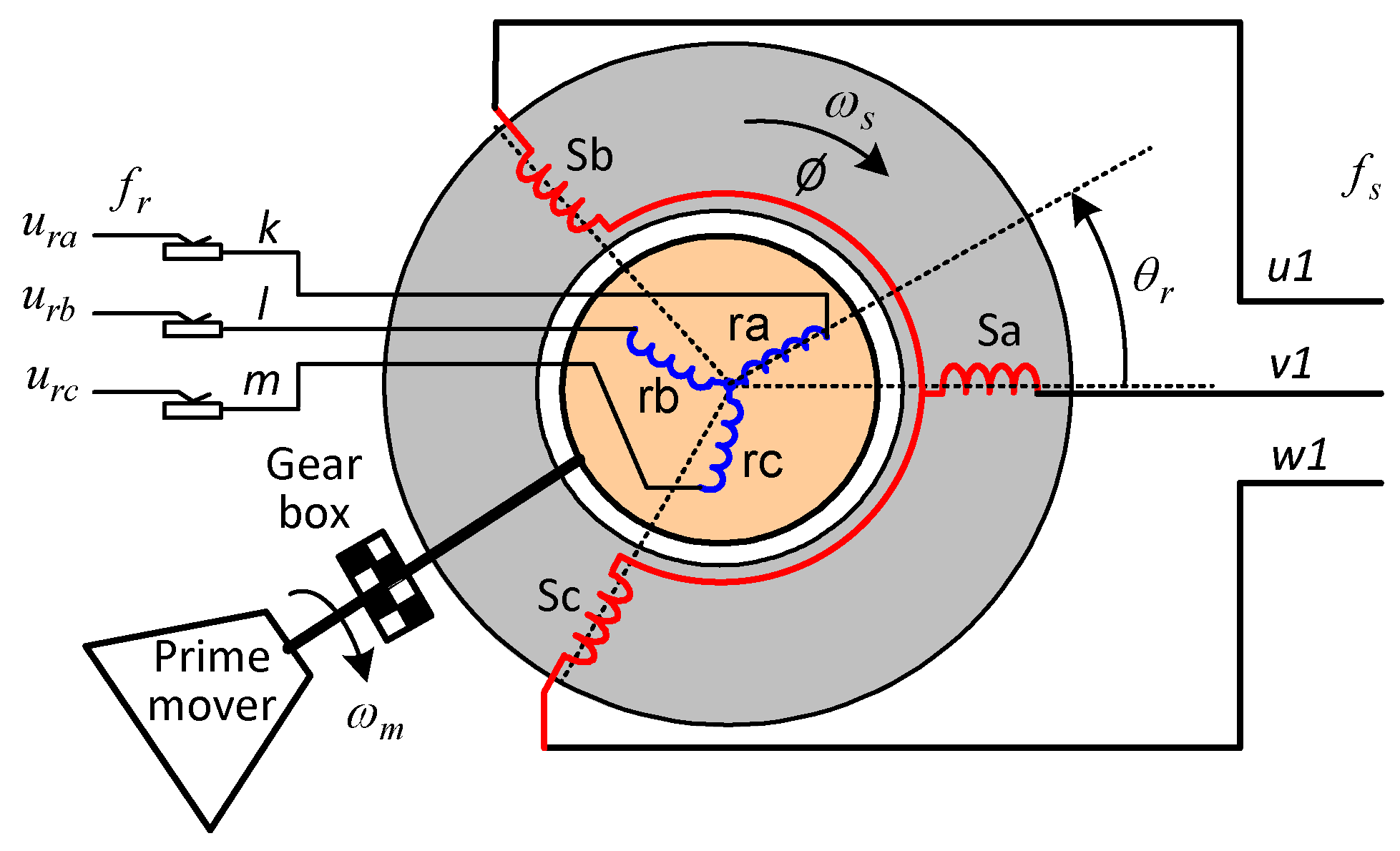
Figure 2.
Operation principle of proposed DFIG system.
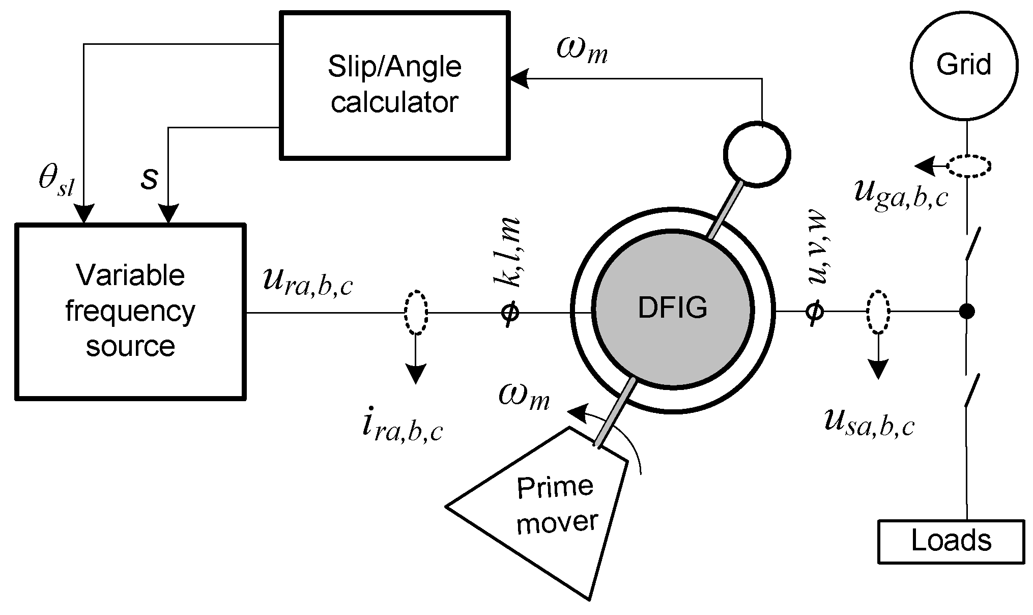
Figure 3.
Initial excitation methods of stand-alone DFIG.
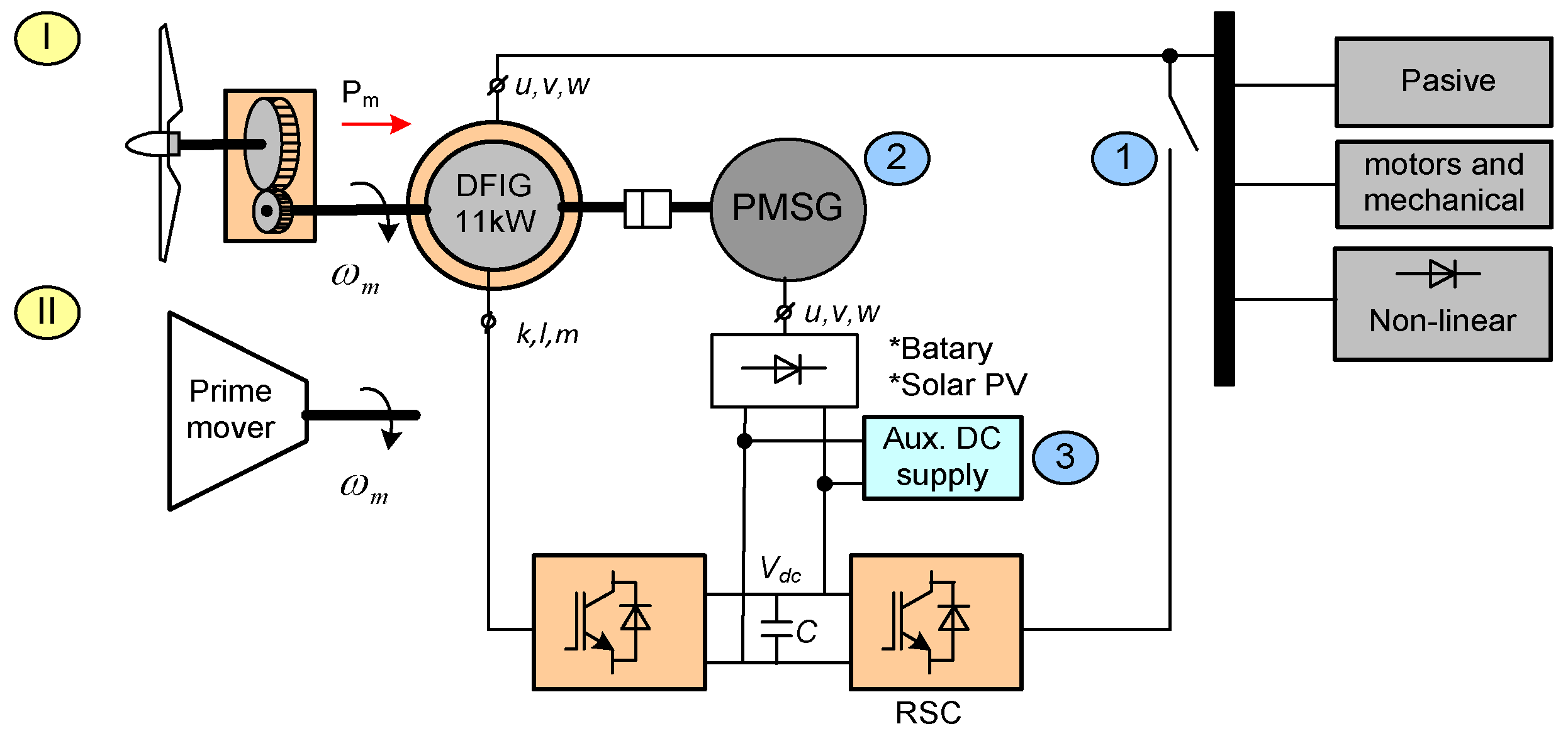
Figure 4.
Equivalent space vector circuit of DFIM.
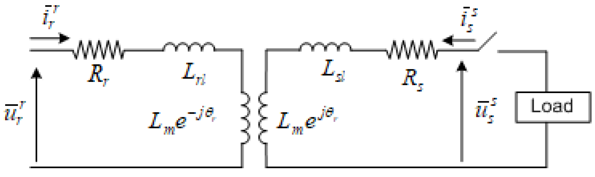
Figure 5.
Equivalent circuit of DFIG stator, and space vectors of stator voltage and current.
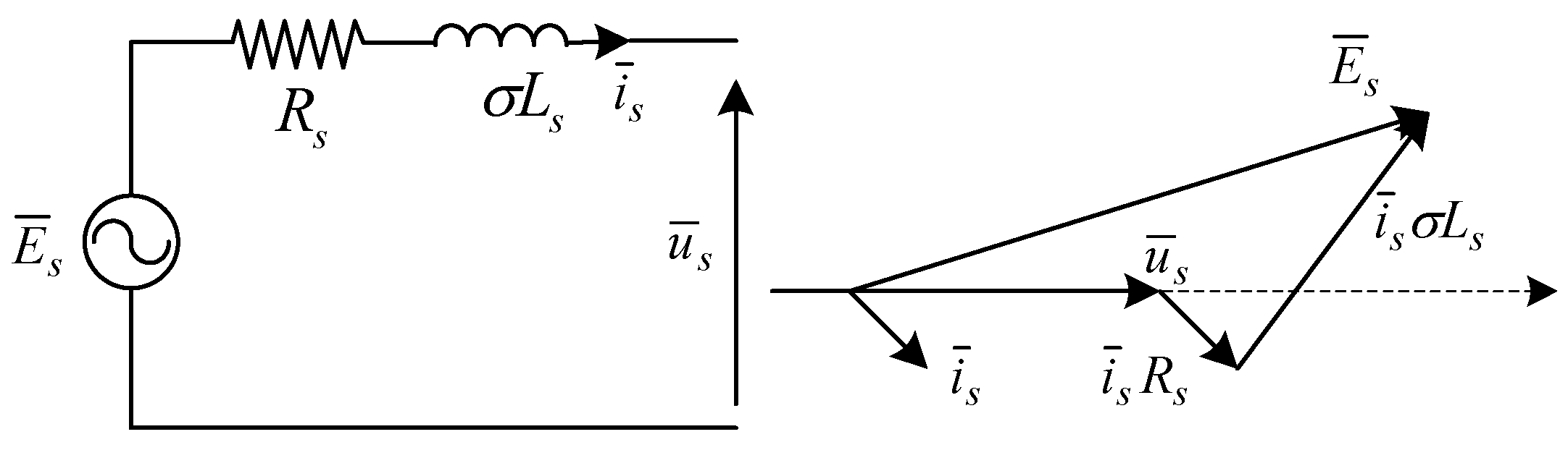
Figure 7.
Simulation model of Grid connected DFIG (for motor and controlled generator).
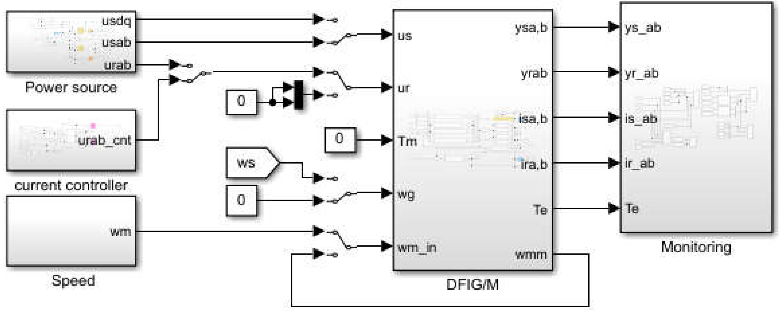
Figure 8.
Simulink model of standalone DFIG a) overall DFIG system above b) stator side model of DFIG below.
Figure 8.
Simulink model of standalone DFIG a) overall DFIG system above b) stator side model of DFIG below.
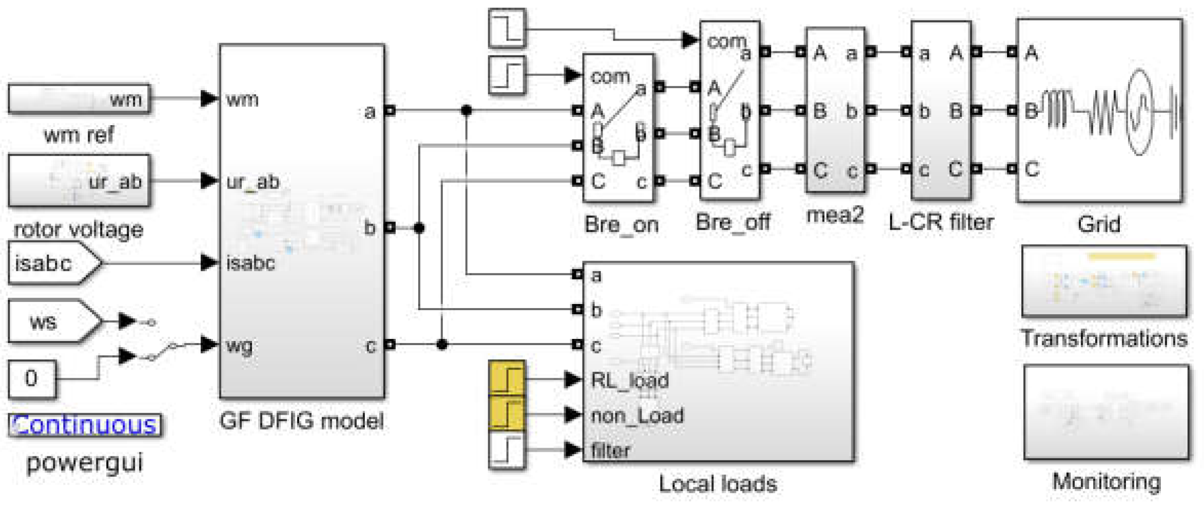
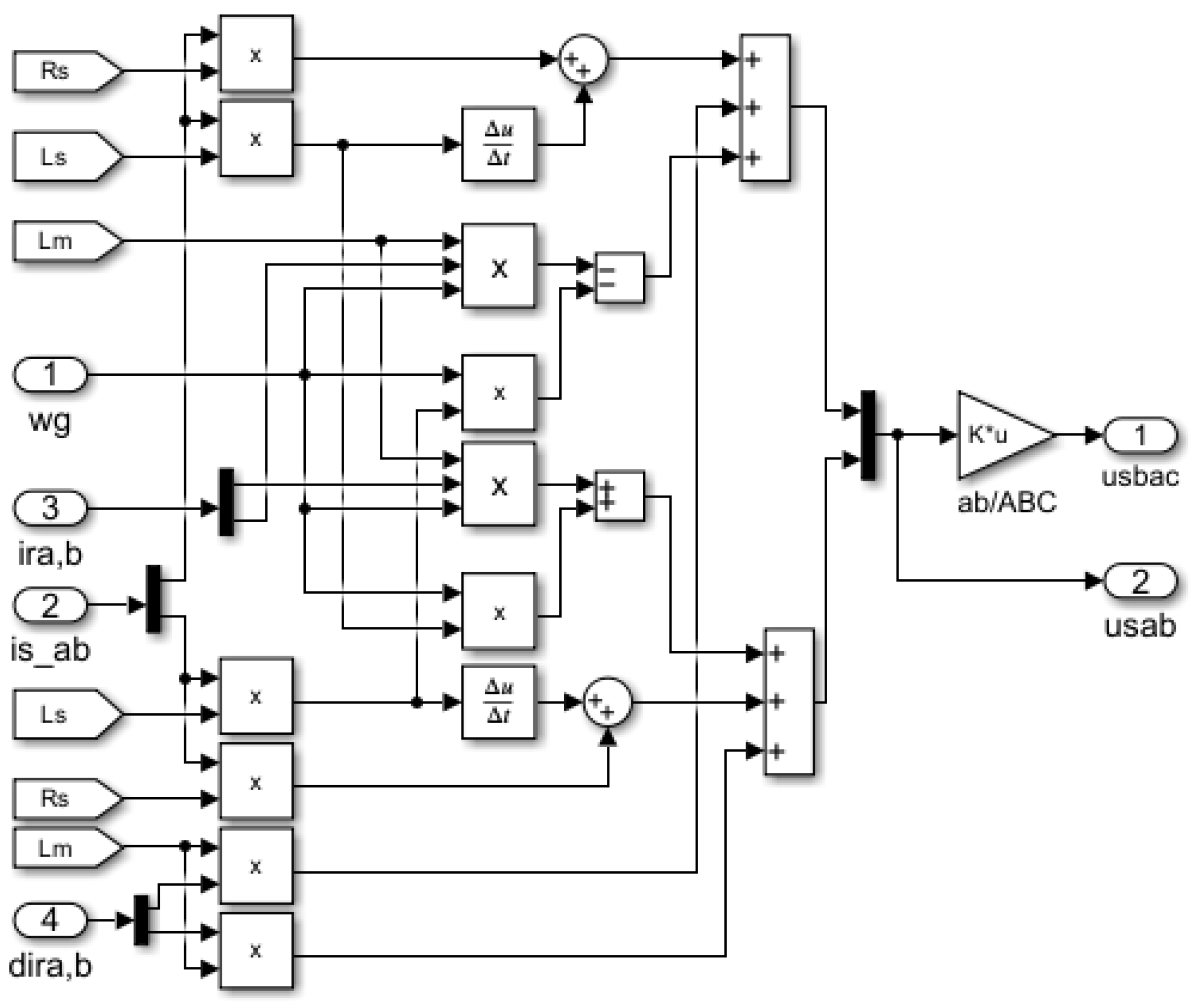
Figure 10.
Simulation results of DFIG with rotor current feedback control.
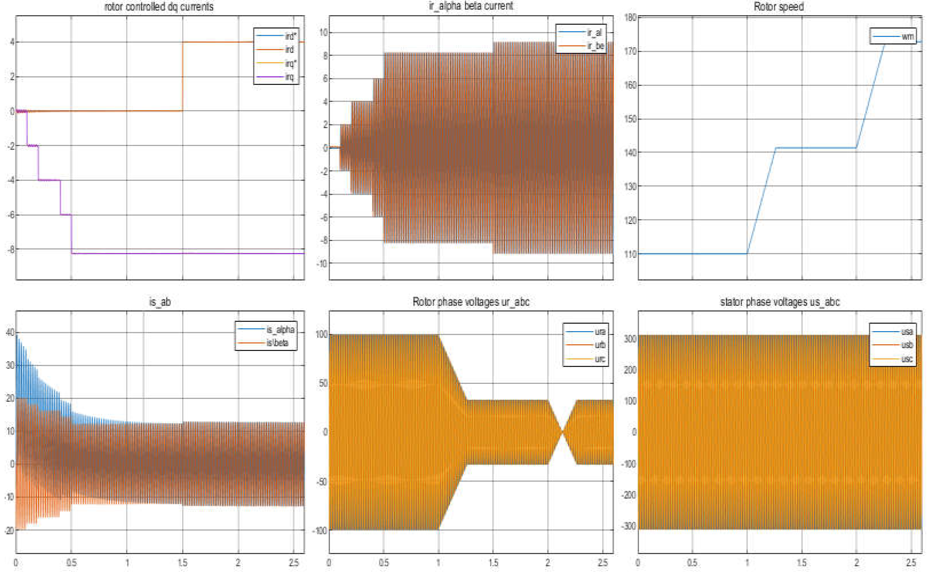
Figure 11.
Simulation results of DFIG in stand-alone operation.
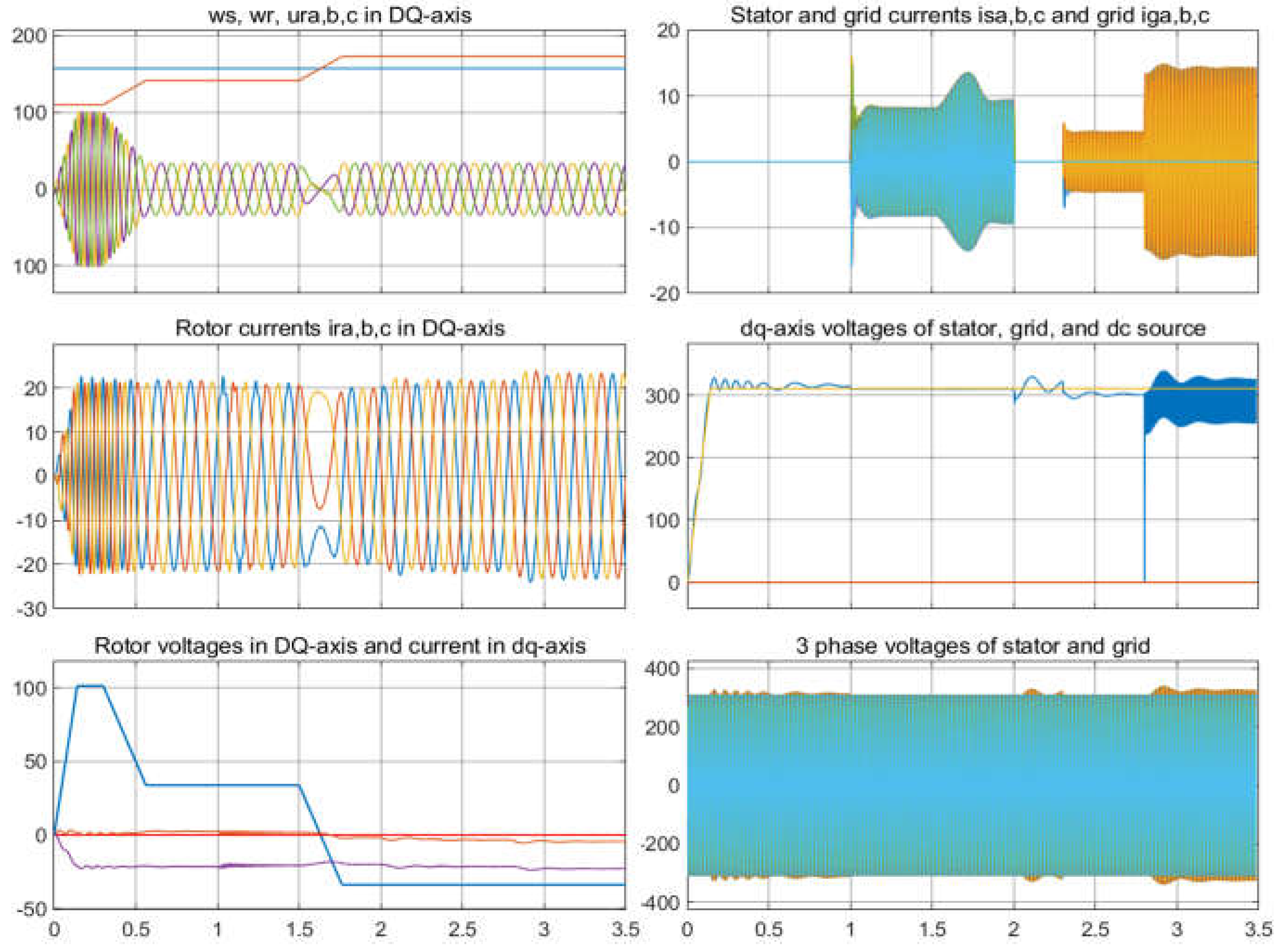
Figure 12.
Simulation of DFIG during connection and disconnection from grid, and various loading in stand-alone mode.
Figure 12.
Simulation of DFIG during connection and disconnection from grid, and various loading in stand-alone mode.

Figure 13.
An image of hardware test setup.
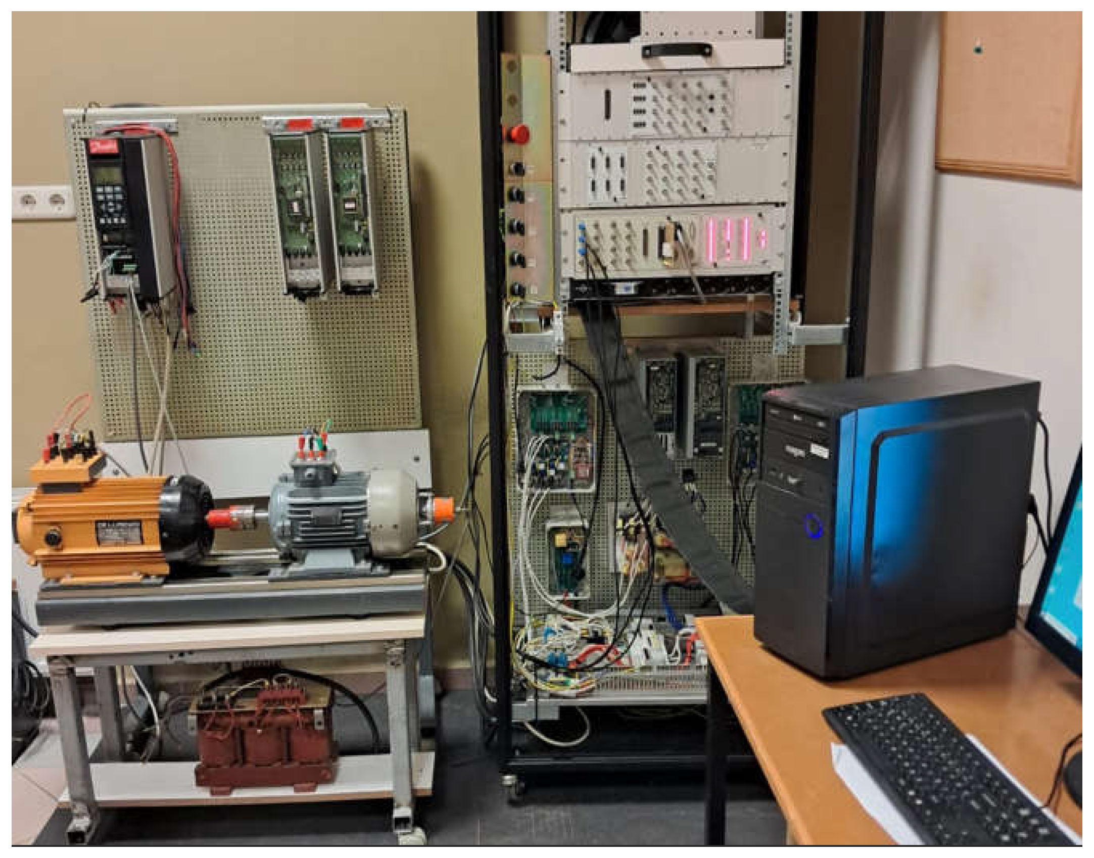
Figure 14.
DFIG test at stand still, nr=0, fr=20Hz, with THPWM.
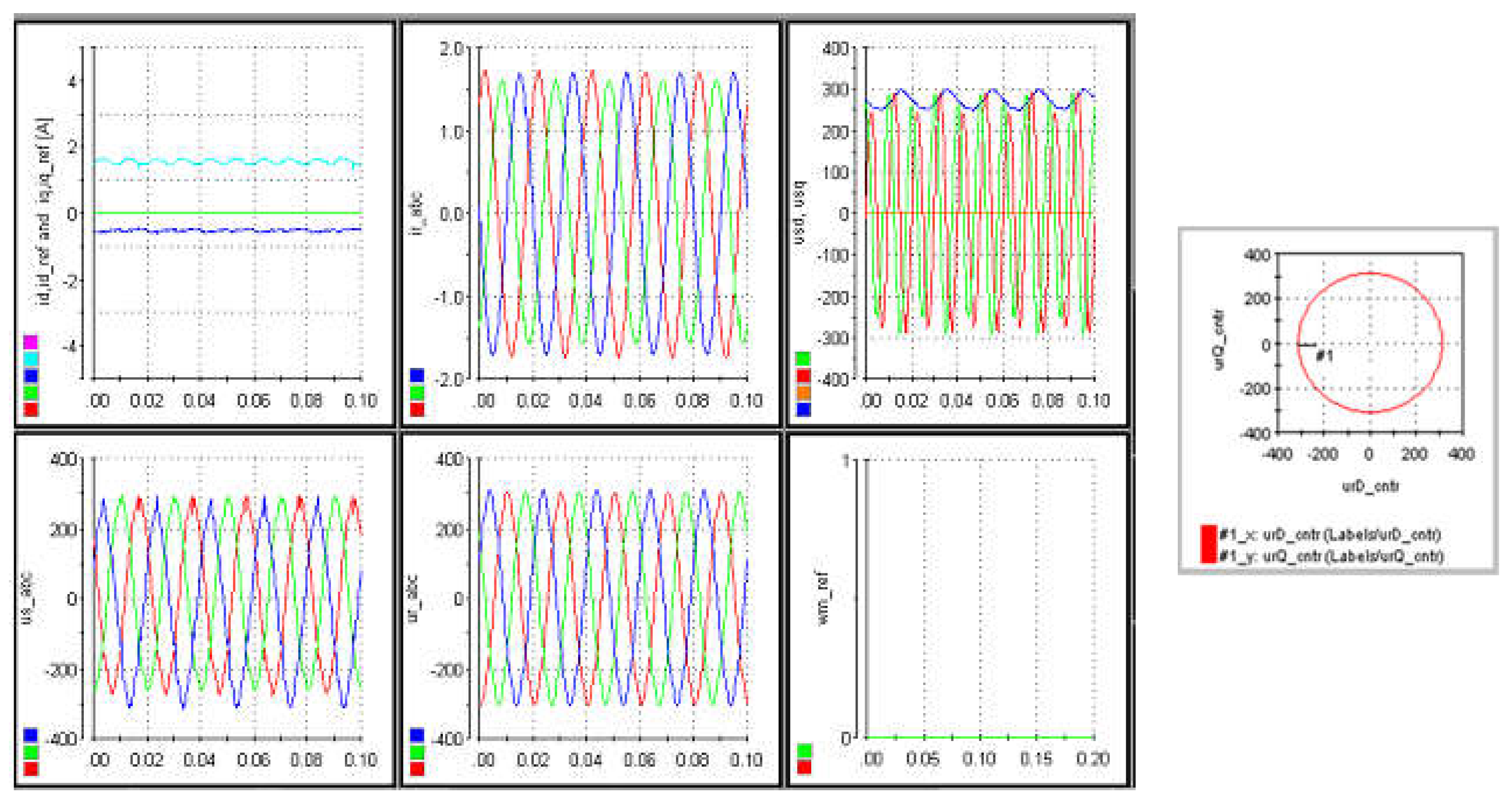
Figure 15.
Experimental results of a DFIG operated stand-alone.
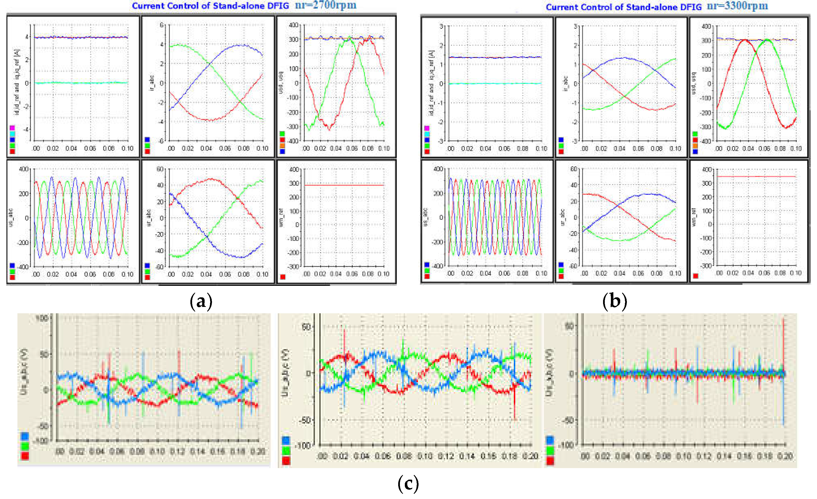

Table 1.
DFIG parameter used in simulated model.
| Quantity | Symbols | Unites |
|---|---|---|
| DFIM Rated power | P | 15 kW |
| Rated stator voltage | usn | 380 V |
| Rated rotor voltage (o. c.) | ur (o) | 565V |
| Rated slip Rated rotor speed range Synchronous speed Stator inductance Rotor inductance Mutual inductance |
±26% nr ns Ls Lr Lm |
600-900 rpm 750 rpm 0.050 H 0.050 H 0.045 H |
| Stator nominal current Rotor nominal current Stator resistance |
isn irn Rs |
55 A 32 A 0,168 Ω |
| Rotor resistance | Rr | 0,199 Ω |
| DC bus voltage | VDC | 565V |
| Pole pair Winding ratio |
p ksr(=ws/wr) |
2 1 |
Disclaimer/Publisher’s Note: The statements, opinions and data contained in all publications are solely those of the individual author(s) and contributor(s) and not of MDPI and/or the editor(s). MDPI and/or the editor(s) disclaim responsibility for any injury to people or property resulting from any ideas, methods, instructions or products referred to in the content. |
© 2024 by the authors. Licensee MDPI, Basel, Switzerland. This article is an open access article distributed under the terms and conditions of the Creative Commons Attribution (CC BY) license (http://creativecommons.org/licenses/by/4.0/).
Copyright: This open access article is published under a Creative Commons CC BY 4.0 license, which permit the free download, distribution, and reuse, provided that the author and preprint are cited in any reuse.


