Submitted:
21 October 2025
Posted:
23 October 2025
You are already at the latest version
Abstract
Current microgrid research primarily focuses on radial topologies and their control strategies, while exploration of the time-domain dynamic behavior of closed-loop controlled microgrids remains relatively insufficient. This research gap makes it difficult to directly observe and deeply analyze the evolution mechanisms of critical phenomena, such as oscillations and instability, when they occur. Therefore, conducting time-domain analysis on closed-loop structures is crucial for revealing system instability mechanisms and ensuring their safe and stable operation. This paper establishes a state-space model for a closed-loop microgrid structure composed of multiple parallel inverters and conducts time-domain stability analysis under grid-connected operation. First, a mathematical model of the closed-loop microgrid system is constructed using state-space equations. Subsequently, time-domain analysis of small-signal stability is performed on the model. By varying key parameters such as the droop coefficient, the influence patterns on system stability are investigated. The results indicate that the droop control coefficient and LC filter parameters exert the most significant impact on system dynamic characteristics. Simulation experiments validate the correctness and effectiveness of the theoretical model. Finally, the time-domain characteristics of this model were further analyzed and validated through simulations. Results demonstrate that the system maintains robust stability under disturbances even in grid-connected mode.
Keywords:
1. Introduction
2. Materials and Methods
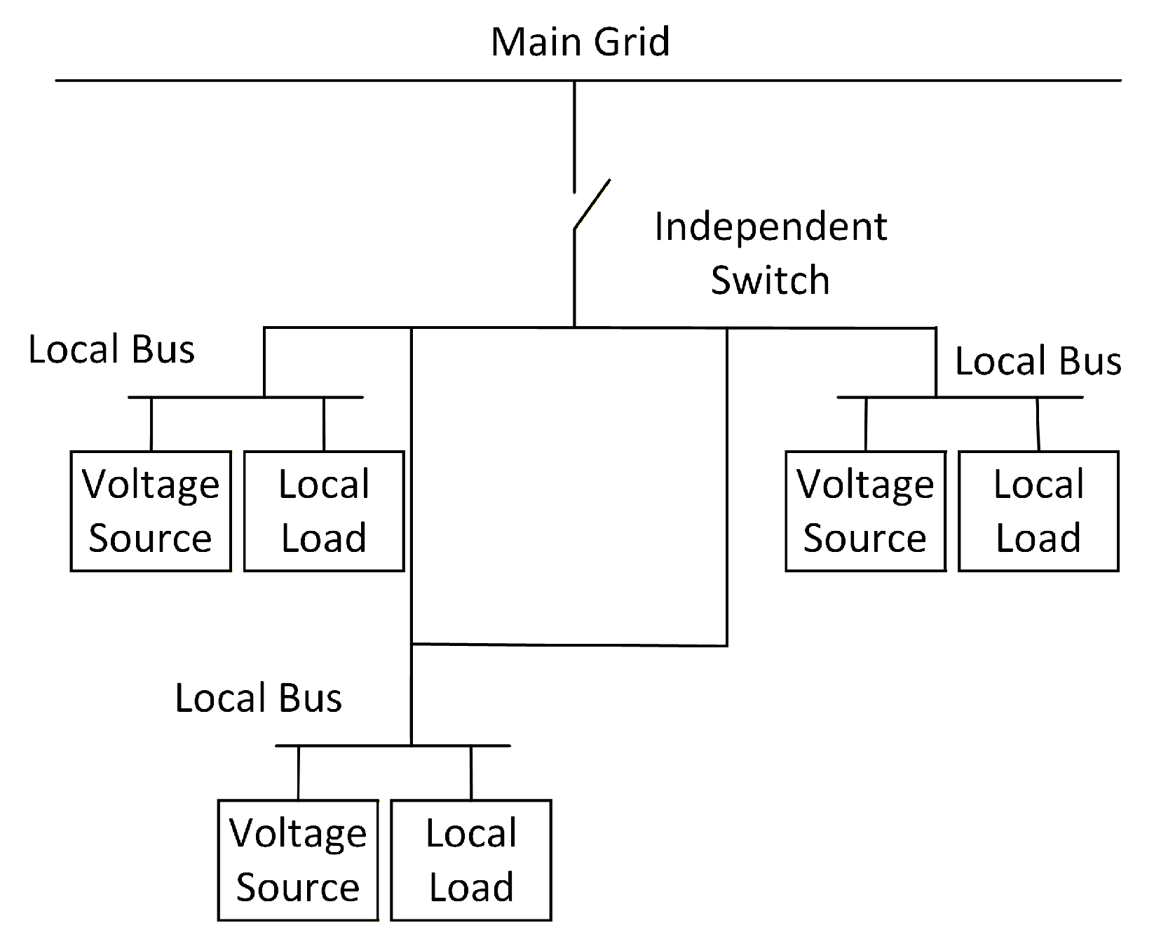
2.1. Model of Microgrid
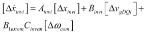
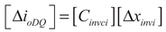
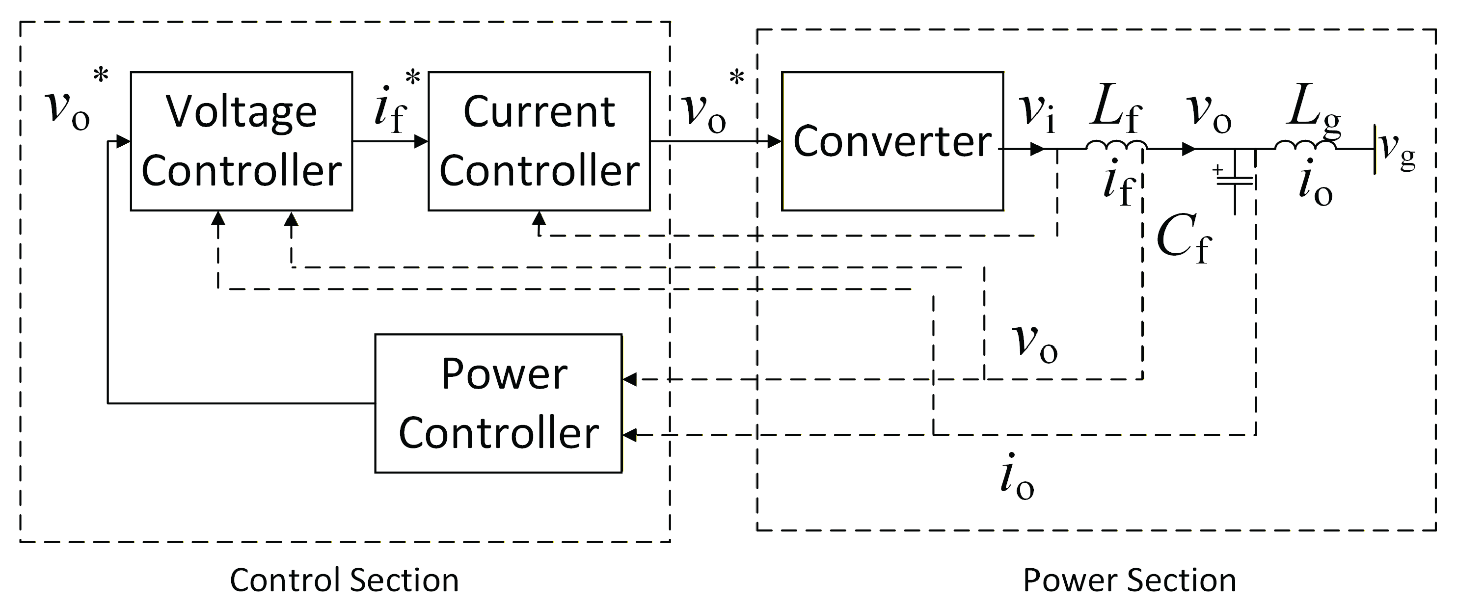
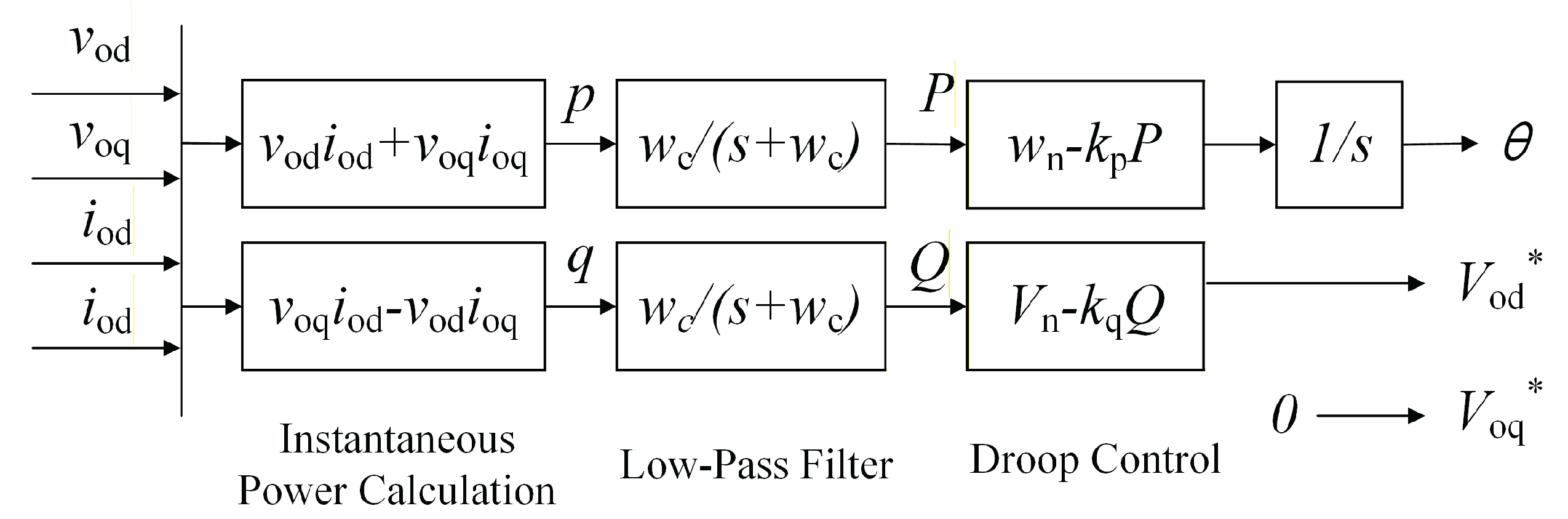
2.1.1. Modeling of a Single Inverter
 (1)
(1)
 (2)
(2)
 (3)
(3)
 (4)
(4)
 (5)
(5)
 (6)
(6)
 (7)
(7)
 (8)
(8)
 (9)
(9)
 (10)
(10)
 (11)
(11)
 (12)
(12)
 (13)
(13)
 (14)
(14)
 (15)
(15)
 (16)
(16)
 (17)
(17)
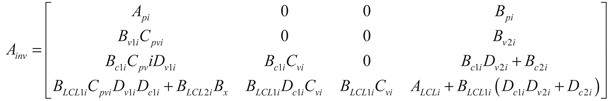
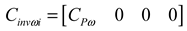
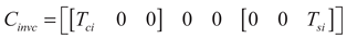
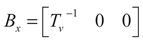
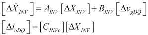
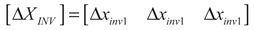
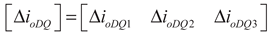
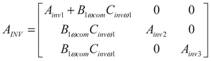
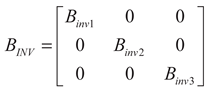
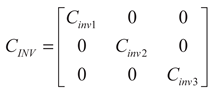
2.1.2. The Combined Model of All Inverters
 (18)
(18)
 (19)
(19)
 (20)
(20)
 (21)
(21)
 (22)
(22)
 (23)
(23)
 (24)
(24)
 (25)
(25)
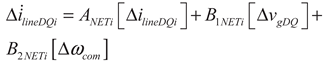
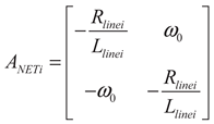
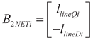
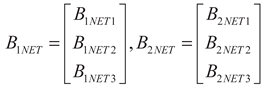
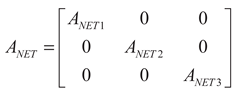
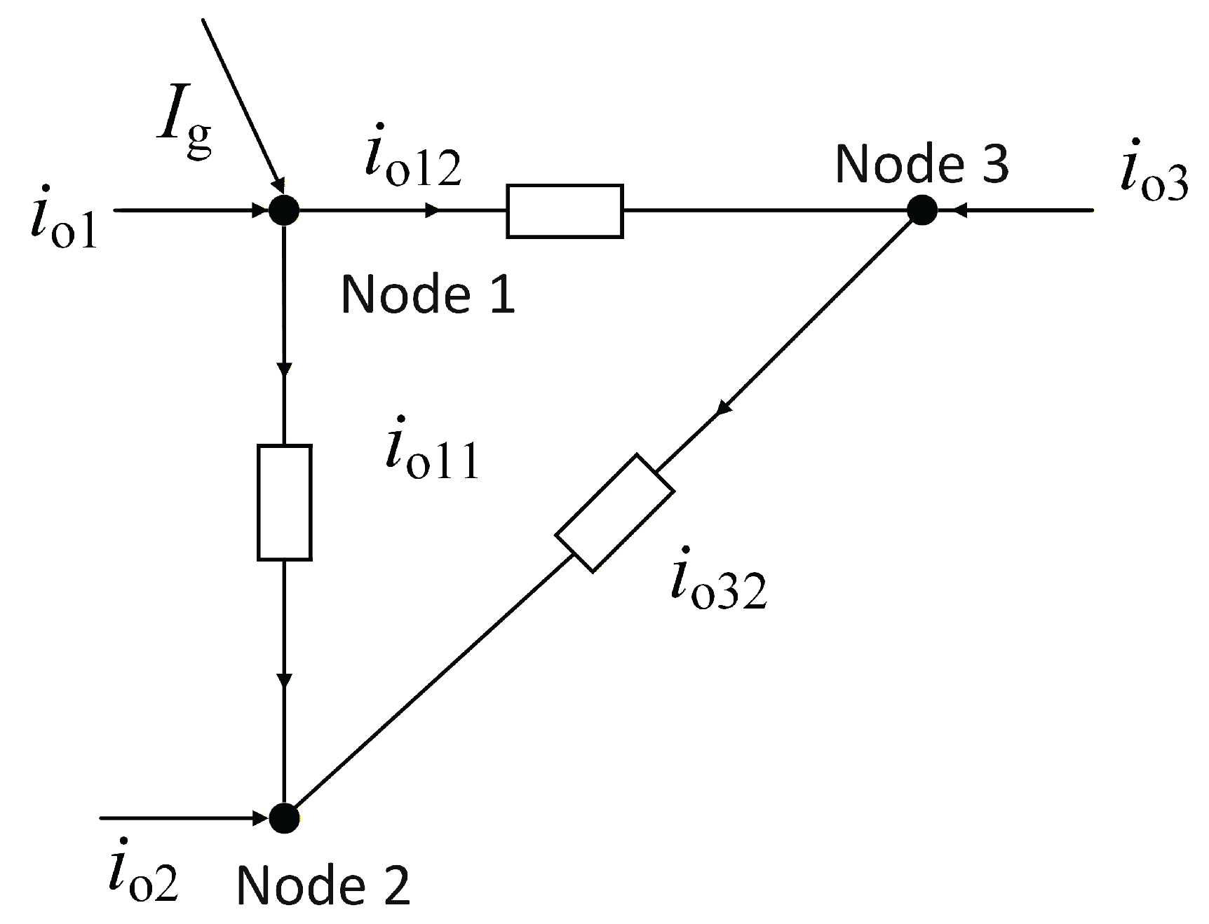
2.1.3. Network Bus Model
 (26)
(26)
 (27)
(27)
 (28)
(28)
 (29)
(29)
 (30)
(30)
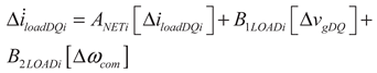
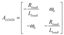
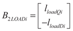
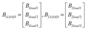
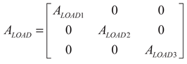
2.1.4. Load Model
 (31)
(31)
 (32)
(32)
 (33)
(33)
 (34)
(34)
 (35)
(35)
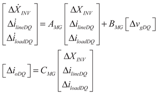
2.1.5. A Complete Microgrid Model
 (36)
(36)
2.2. Stability Analysis
3. Results & Discussion
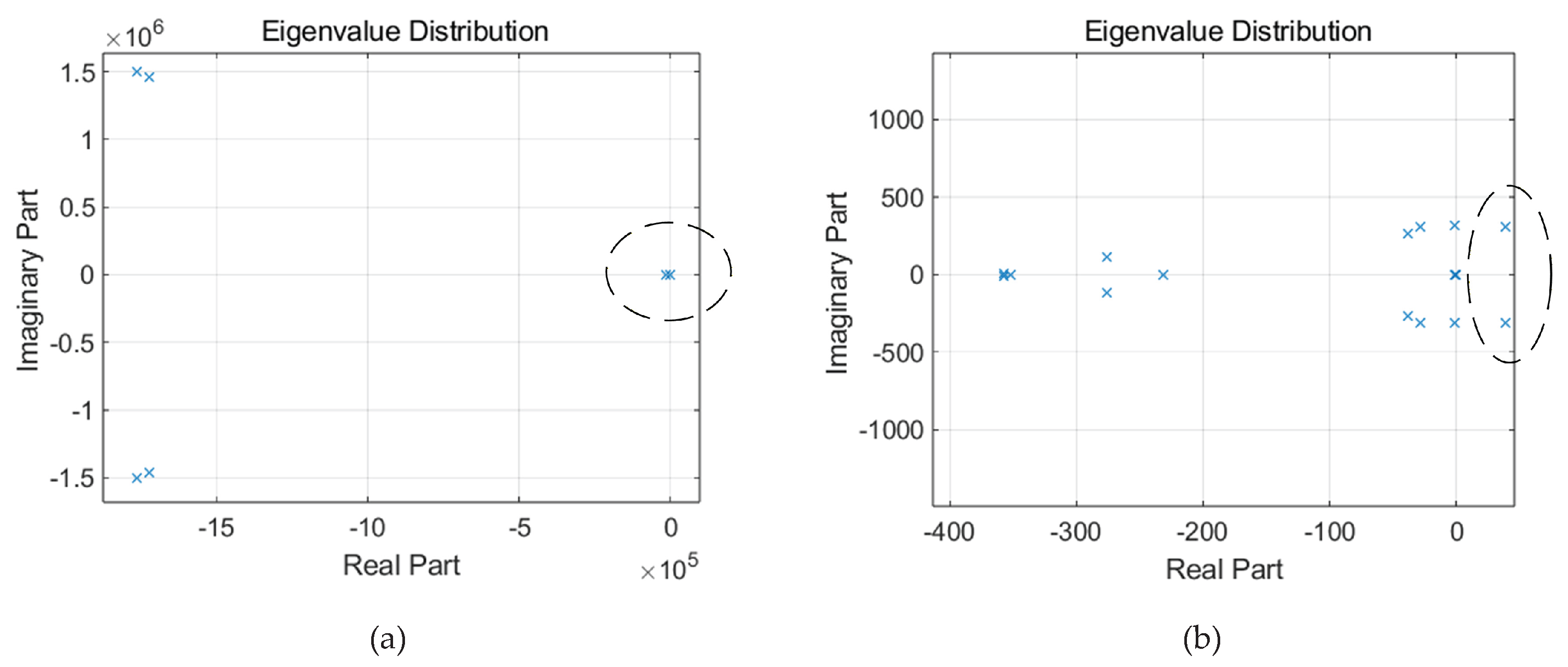
3.1. Stability Analysis
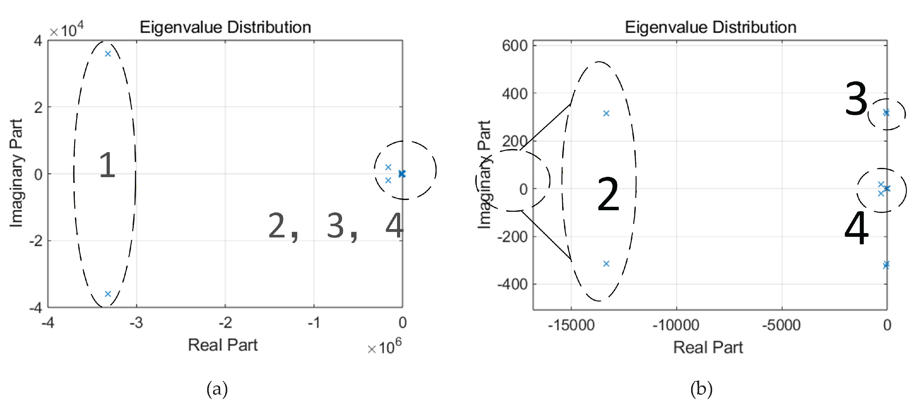
3.1.1. Eigenvalue Analysis
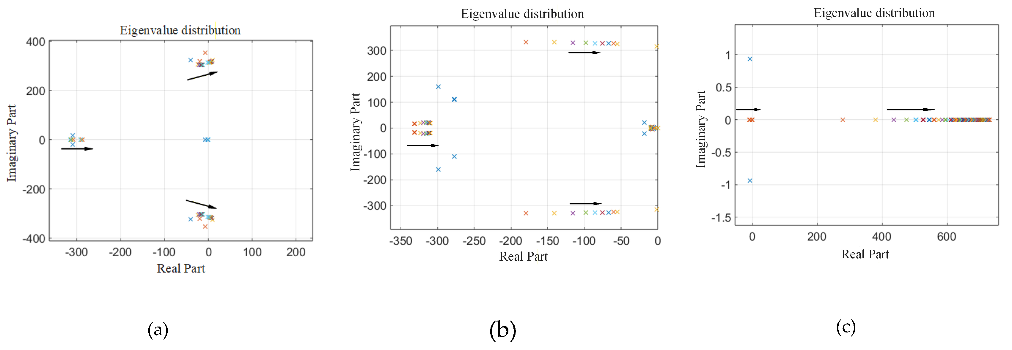
3.1.2. Sensitivity Analysis
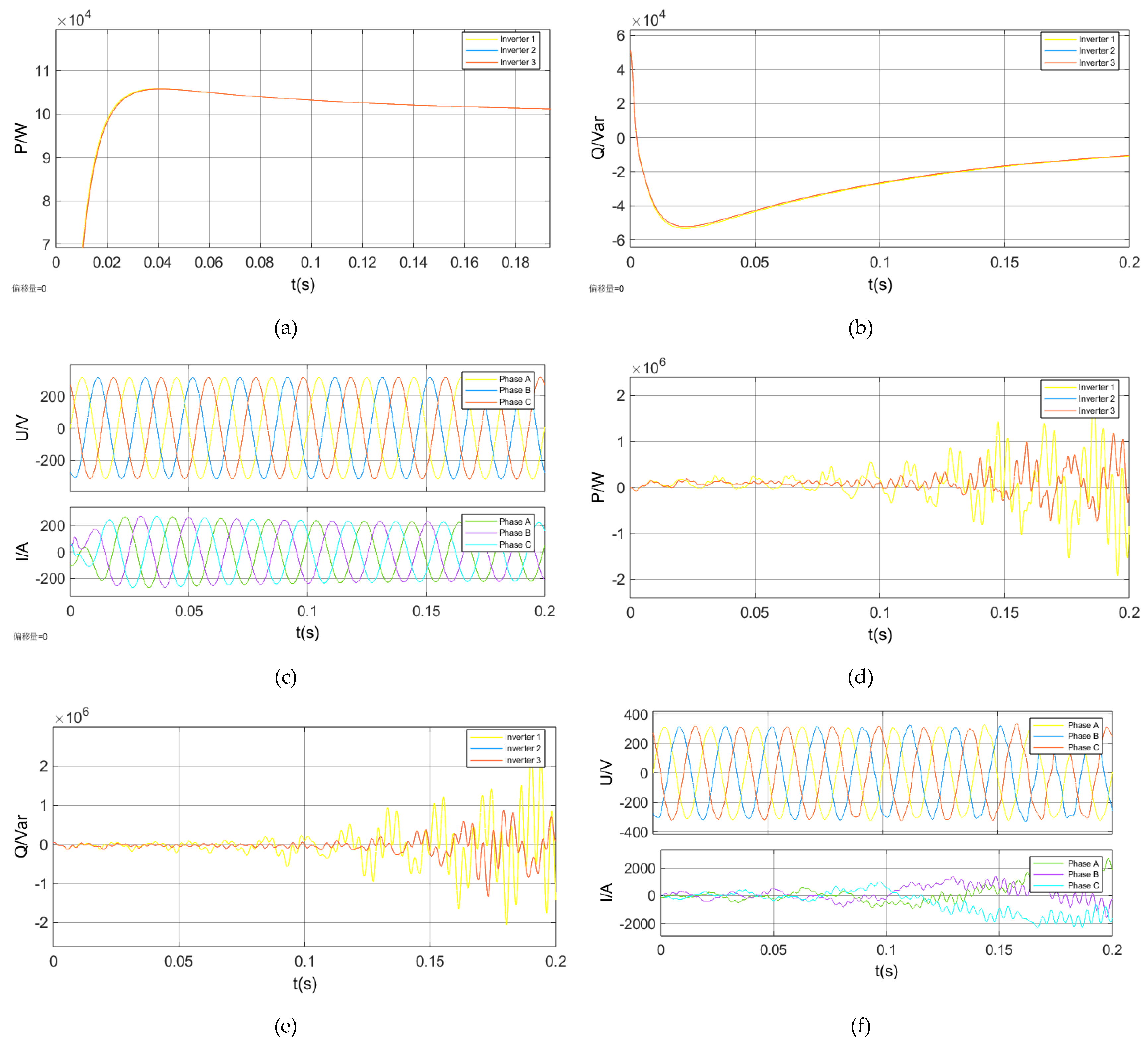
3.1.3. Verification of the Model
3.2. Time-Domain Stability Analysis
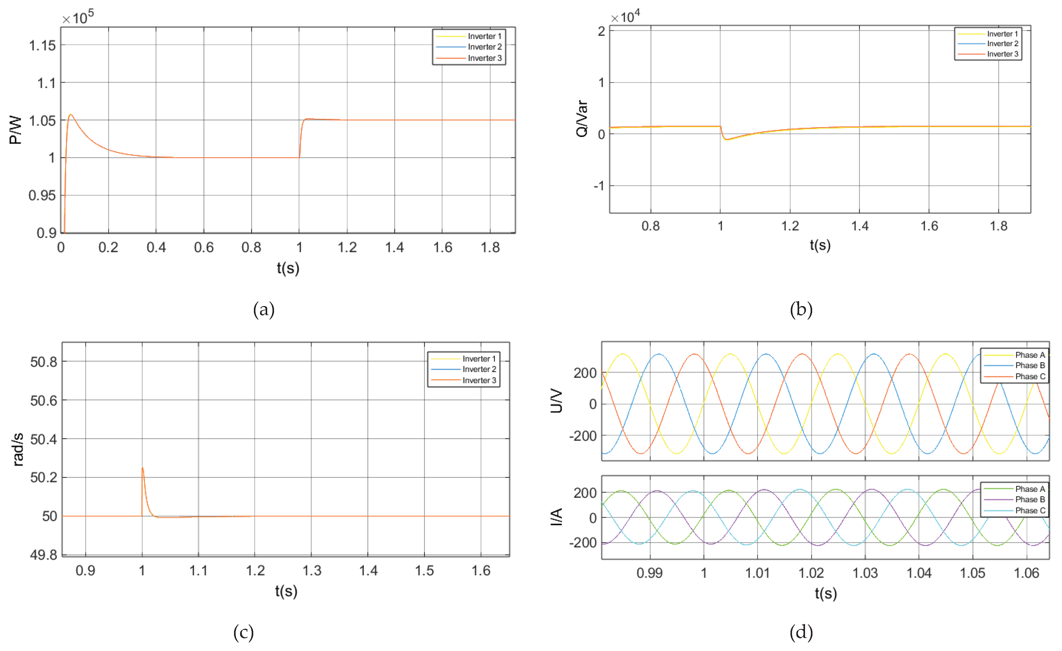
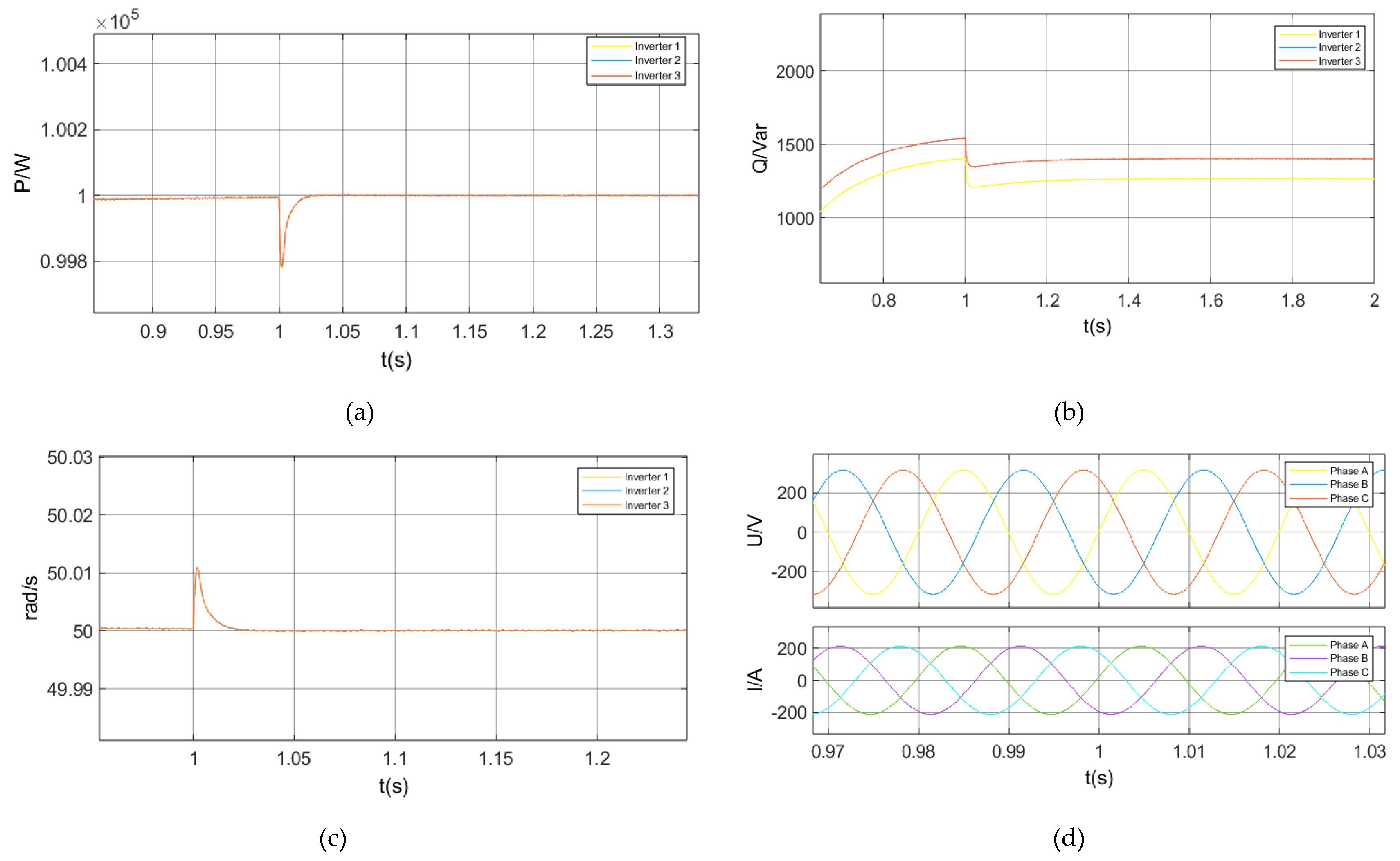
3.2.1. Case 1: A 5% Step Increase in the Active Power Command in Droop Control
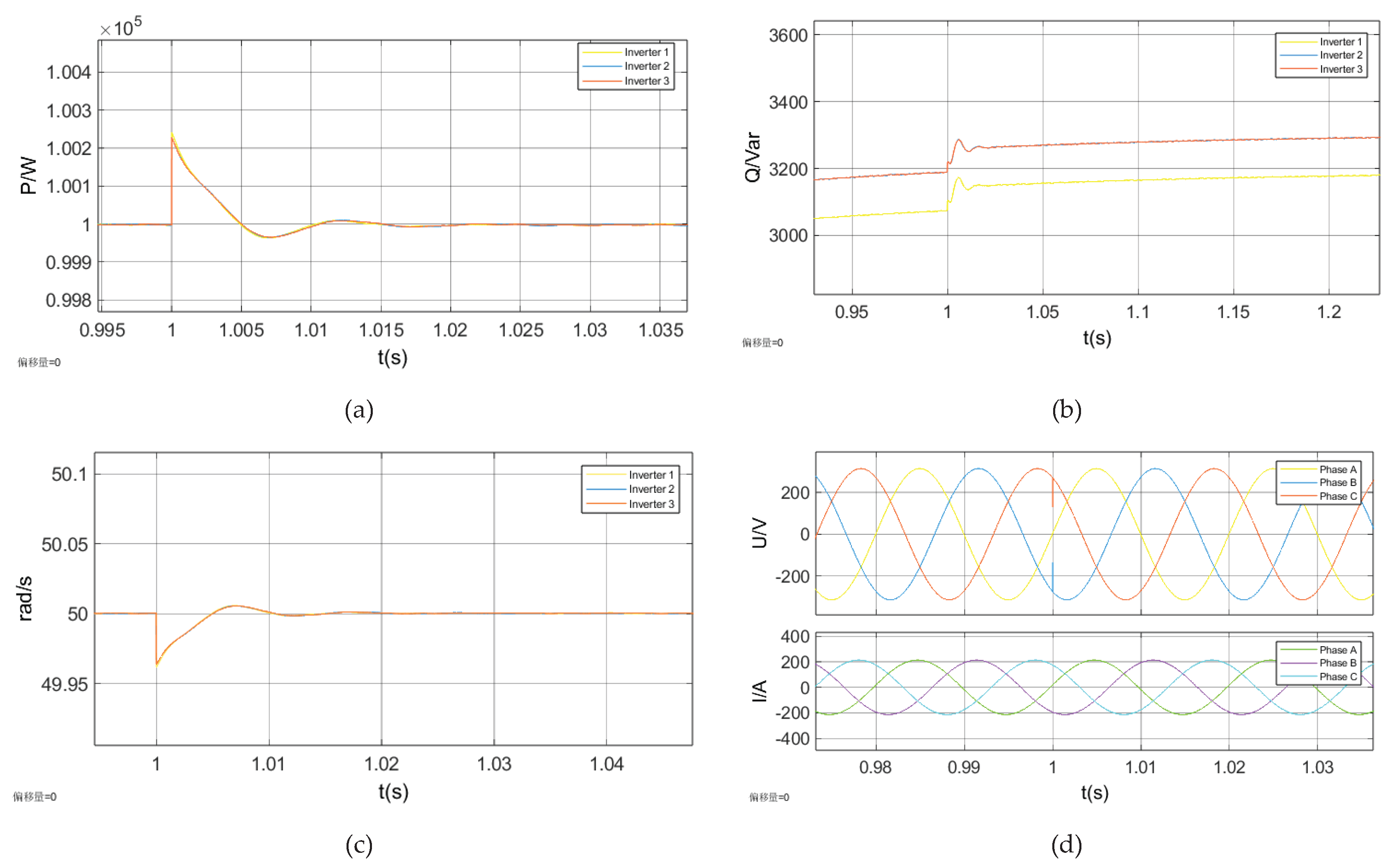
3.2.3. Case 3: A 5% Step Increase in the Active Power Load at the PCC in Droop Control
4. Conclusions
References
- S. A. Arefifar; M. Ordonez; Y. Mohamed. Energy management in multi-microgrid systems — development and assessment. 2017 IEEE Power & Energy Society General Meeting, Chicago, IL, USA, 2017, 1-1.
- Farzin Hossein; M. Fotuhi-Firuzabad; M. Moeini-Aghtaie. Enhancing Power System Resilience Through Hierarchical Outage Management in Multi-Microgrids. IEEE Trans. Smart Grid. 2016, 7, 2869–2879. [Google Scholar] [CrossRef]
- T. Meng; Z. Lin; Y. Wan; Y. A. Shamash. An Output Regulation Approach to Distributed Voltage Regulation of Multiple Coupled Distributed Generation Units in DC Microgrids, in 2022 American Control Conference (ACC), Atlanta, GA, USA, 2022, 4534-4539.
- Dong Zhaoyang; Zhao Junhua; Wen Fushuan; XUE Yusheng. From smart grid to energy Internet: Basic concept and research framework. AEPS 2014, 38, 15, 1–11. [Google Scholar]
- Ma Zhao; Zhou Xiaoxin; Shang Yuwei; SHENG Wanxing. Exploring the Concept, Key Technologies, and Development Model of Energy Internet. PST 2015, 39, 113014–3022. [Google Scholar]
- J. de la Cruz; Y. Wu; J. E. Candelo-Becerra; J. C. Vásquez; J. M. Guerrero. Review of Networked Microgrid Protection: Architectures, Challenges, Solutions, and Future Trends. CSEEJ POWER ENERGY 2024, 10, 448–467. [Google Scholar]
- Sui X, Tang Y, He H; Wen, J. Energy-Storage-Based Low-Frequency Oscillation Damping Control Using Particle Swarm Optimization and Heuristic Dynamic Programming. IEEE Trans. Power Syst 2014, 29, 2539–2548. [Google Scholar] [CrossRef]
- Z Zeng; R ZHAO; Lü Z; L Ma. Impedance Reshaping of Grid-tied Inverters to Damp the Series and Parallel Harmonic Resonances of Photovoltaic Systems. In Proceedings of the CSEE. 2014, 34, 45747–4558. [Google Scholar]
- LI Junjie; LÜ Zhenyu; WU Zaijun; LIU Haijun; YANG Shihui. Adaptive switching strategy of AC/DC hybrid microgrid operating mode based on the power electronic transformer. Electric Power Automation Equipment 2020, 40, 126–131+138. [Google Scholar]
- SUN Zhenao; YANG Zilong; WANG Yibo; XU Hongbo. A Hybrid Islanding Detection Method for Distributed Multi-inverter Systems. In Proceedings of the CSEE 2016, 36, 3590–3597+3378. [Google Scholar]
- GU Xiaofeng; YUAN Xufeng; ZHENG Huajun; XIONG Wei. Review of AC/DC hybrid microgrid stability analysis and its enhancement measures. Distribution & Utilization 2025, 42, 8–20. [Google Scholar]
- Guerrero, Josep M. et al. Advanced Control Architectures for Intelligent Microgrids—Part I: Decentralized and Hierarchical Control. IEEE Trans. Ind. Electron 2013, 60, 1254–1262. [Google Scholar] [CrossRef]
- Xu, Yuqin; Fang, Nan. Control strategy research and simulation analysis of an independent optical storage microgrid based on voltage stabilizing control. Power System Protection and Control 2020, 48, 67–74. [Google Scholar]
- Feng Wei; Sun Kai; Guan Yajuan; Josep M. Guerrero; XIAO Xi. An Active Harmonic Grid-Connecting Current Suppression Strategy for Hierarchical Control-Based Microgrid. Transactions of China Electrotechnical Society 2018, 33, 1400–1409. [Google Scholar]
- M. Li, X. Zhang, X. Fu, H. Geng, and W. Zhao. Stability Studies on PV Grid-connected Inverters under Weak Grid: A Review. Chinese Journal of Electrical Engineering 2024, 10, 1–19. [Google Scholar] [CrossRef]
- Lopes, J. A. Pecas; C. L. Moreira; A. G. Madureira. Defining control strategies for Micro Grids islanded operation. IEEE Trans. Power Syst. 2006, 21, 916–924. [Google Scholar] [CrossRef]
- Liu Xu; Zhang Guoju; Pei Wei; ZHU Enze; ZHANG Xue. Current status and development trends of grid-type converters. Acta Energiae Solaris Sinica 2024, 45, 101–111. [Google Scholar]
- HUANG Xianmiao1; SHAO Yichi; GONG Yu; LIU Di; ZHU Xuesen; LUO Jiasen. Control technology for grid-forming energy storage under unbalanced working conditions of weak current networks. Thermal Power Generation 2024, 53, 59–67. [Google Scholar]
- WU Yuanyao; XIAO Shiwu. Static Voltage Stability Analysis of New Energy Islanded Microgrids Supported by Grid-forming Energy Storage. PST.
- M. Lu, Y. Yang; B. Johnson; and F. Blaabjerg. An Interaction-Admittance Model for Multi-Inverter Grid-Connected Systems. TPE 2019, 34, 7542–7557. [Google Scholar]
- N. Pogaku; M. Prodanovic; T. C. Green. Modeling, Analysis, and Testing of Autonomous Operation of an Inverter-Based Microgrid. TPE 2007, 22, 613–625. [Google Scholar]
- He Jinwei; Yun Wei Li. An Enhanced Microgrid Load Demand Sharing Strategy. TPE 2012, 27, 3984–3995. [Google Scholar]
- SHI Jie; ZHENG Zhanghua; AI Qian. Modeling of DC micro-grid and stability analysis. Electric Power Automation Equipment 2010, 30, 86–90. [Google Scholar]
- Wang Shuya; Su Jianhui; Yang Xiangzhen; DU Yan. A review of the small signal stability of the microgrid. Electr. Eng 2016, 11, 39–45. [Google Scholar]
- LIU Hong; BAO Mingyang; LU Shaohan; DUAN Qing; SHENTU Leixuan; HUANG Yuanping. Coordinated operation method of the distribution network and multiple microgrids considering network reconfiguration. Electric Power Automation Equipment 2025, 45, 114–121. [Google Scholar]
- Xiang Yang; Fu Ming; Zhang Aifang; DOU Xiaobo; JIAO Yang; YANG Yeqing. Small signal stability analysis of AC/DC hybrid microgrid under isolated island operation. Electric Power Construction 2017, 38, 96–105. [Google Scholar]
- Zheng Jinghong; Li Xingwang; Wang Yanting; ZHU Shouzhen; WANG Xiaoyu; ZHU Hongbo. Small-signal stability analysis of a microgrid switching to islanded mode. Automation of Electric Power Systems 2012, 36, 25–32. [Google Scholar]

| Classification of Parameters | Parameter Symbol | Base Value |
|---|---|---|
| System Base Parameters | Rated Capacity, S(kVA) | 50 |
| Rated Line-to-Line Voltage, V(V) | 380 | |
| Rated Frequency, f(Hz) | 50 | |
| Inverter Unit | DC-Link Voltage, V_dc(V) | 220 |
| LC Filter | Inverter-Side Inductance, L1(H) | 3e-3 |
| Filter Capacitance ,Cf(F) | 20e-6 | |
| Droop Control | Active Power-Frequency Droop Coefficient,m(rad/W*s) | 3.14e-4 |
| Reactive Power-Voltage Droop Coefficient,n(V/Var) | 1e-3 | |
| Other parameters | Grid-Side Inductance,L2(H) | 7e-3 |
| Line inductance,Lline(H) | 3e-5 | |
| Line resistance,Rline(Ω) | 4e-5 |
| Number of inverters ( i = 1,2,3) | Steady-state operating point data |
|---|---|
| Steady-state angular frequency(/rad·s-1) | 314.16214.9527 |
| The phase difference relative to the common rotating coordinate system (i/rad) | (0,0.0066,-5.59e-8) |
| Output voltage in common rotating coordinate system ( VgDi , VgQi )/V | (214.95,-13.11) (214.89,-12.95) (-214.95,-13.11) |
| Inverter output voltage( Vodi, Voqi ) / V | (214.89,-12.95) (-214.95,-13.11) (214.89,-12.95) |
| Inverter output current ( Iodi, Ioqi ) / A | (214.89,-12.95) (-214.95,-13.11) (214.89,-12.95) |
| Inverter-side current ( Ifdi, Ifqi ) / A | (215.15,84.31) (214.99,84.49) (215.07,84.22) |
| Inverter local load current (IloadDi, IloadQi ) / A | (0.0772,-0.01) (0.0767,-0.01) (0.0767,-0.01) |
| Line current (IlineDi, IlineQi ) / A | (215.35,0.032) (0,0) (215.35,0.032) |
| Parameters | Kpc | Kpv |
|---|---|---|
| Stable Condition | 95 | 3 |
| Unstable Condition | 0.95 | 30 |
Disclaimer/Publisher’s Note: The statements, opinions and data contained in all publications are solely those of the individual author(s) and contributor(s) and not of MDPI and/or the editor(s). MDPI and/or the editor(s) disclaim responsibility for any injury to people or property resulting from any ideas, methods, instructions or products referred to in the content. |
© 2025 by the authors. Licensee MDPI, Basel, Switzerland. This article is an open access article distributed under the terms and conditions of the Creative Commons Attribution (CC BY) license (http://creativecommons.org/licenses/by/4.0/).


