
Submitted:
10 November 2024
Posted:
11 November 2024
You are already at the latest version
Abstract
Wireless Sensor Networks are used in an ever increasing range of applications, thanks to their ability to monitor and transmit data related with ambient conditions at almost any area of interest. The optimization of coverage and the assurance of connectivity are fundamental for the efficiency and consistency of Wireless Sensor Networks. Optimal coverage guarantees that all points in the field of interest are monitored, while the assurance of the connectivity of the network nodes assures that the gathered data are reliably transferred among the nodes and the base station. In this research article a based on Particle Swarm Optimization novel algorithm to assure coverage and connectivity in Wireless Sensor Networks is proposed. The objective function is derived from energy function minimization methodologies commonly applied in bounded space circle packing problems. The performance of the novel algorithm is not only evaluated through both simulation and statistical tests that demonstrate the efficacy of the proposed methodology but also compared against that of relative algorithms. Finally, concluding remarks are drawn on the potential extensibility and actual use of the algorithm in real-world scenarios.
Keywords:
wireless sensor networks
; coverage
; k-coverage
; connectivity
; 1-connectivity
; optimization
; circle packing
; particle swarm optimization
1. Introduction
A wireless sensor network (WSN) is a group of devices that communicate wirelessly while being disseminated over an area of interest. Typically, it contains a number of sensor nodes along with at least one sink node usually referred as base station. The sensor nodes are micro electromechanical systems able to sense ambient conditions, collect and process the relative information and transmit the corresponding data to other nodes or/and the base station. The base station is a device which, thanks to its enhanced energy, computational, and communication resources, is able to process received from the network nodes, perform supervisory control of the WSN, and communicate with the end user and/or other networks [1,2]. The architecture of a typical WSN is illustrated in Figure 1.
A WSN, taking advantage of the combined abilities of the nodes and the base station(s) that contains, is capable of both monitoring the ambient conditions at areas of interest of almost any kind and transmit related information to destinations no matter how much distant they are. For this reason, WSNs have been the basis of the Internet of Things (IoT) and support several sectors of human activities such as industry, flora and fauna, environment, healthcare, military and urban [3]. Consequently, the already wide list of WSNs’ applications keeps on continuously growing [4,5,6,7,8,9,10,11,12,13,14].
On the other hand, WSNs suffer due to not only inborn problems of wireless communications, but also severe restrictions of the sensor nodes regarding their resources for energy, storage and processing, not to mention various other application-related difficulties. Hence, plentiful scientific challenges and issues that need to be addressed are generated [15]. This is why, the development of optimization and multiobjective optimization algorithms is necessitated [16]. These algorithms aim to enhance the operation of WSNs regarding correspondingly individual and several performance metrics subject to a set of constraints such as coverage and connectivity optimization [17,18,19], energy sustainability [20], congestion avoidance [21], quality of service attainment [22], security provision [23], data aggregation [24], fault tolerance [25], and node localization [26].
This research article focuses on coverage and connectivity optimization. Actually, the coverage optimization problem can be identified as the problem of locating a certain quantity of sensor nodes, which have a given sensing range, in the finest arrangement pursuing the maximization of the area covered by them and consequently minimize the coverage holes. Specifically in WSNs, three kinds of coverage may be recognized, which namely are area (or regional) coverage, target (or point) coverage, and barrier (or path) coverage. Area coverage refers to the monitoring of an area of interest in a pattern that guarantees that within this area all points are all the time observed. Target coverage denotes the unceasing monitoring of specific points of interest. Barrier coverage refers to the ability to always detect the movement across a barrier of sensor nodes [27]. Actually, the mostly investigated coverage optimization problem in WSNs is that of area coverage. It can be stated either as 1-coverage or as k-coverage (where k is an integer greater than 1), depending on the minimum number of sensor nodes that always must monitor the specific area of interest simultaneously.
Apparently, area coverage maximization is pursued in every WSN containing a definite number of sensor nodes. Nevertheless, the area coverage problem in WSNs is recognized as a non-trivial research problem, because there are several issues that influence area coverage [28]. For instance, the distribution of sensor nodes within the area of interest can be either arbitrary or deterministic. Similarly, the sensing area may be either probabilistic or deterministic. Also, the sensitivity of the sensor nodes may be either probabilistic or Boolean. Likewise, the communication range of the network nodes may be either variable or invariable. Moreover, the coverage pattern taken on may be either distributed or centralized. Furthermore, sensor nodes in a network may be either static or mobile. At the same time, the optimal distribution of sensor nodes in a network that maximizes coverage may cause connectivity losses to the sensor nodes of this network.
The goal of this research article is to find, under constraints, the optimal spatial deployment of a predetermined set of sensor nodes of varying sensing and communication capabilities as to maximize the sensed coverage of a specified area. One constrain might be that of the k-coverage of the specific area points, meaning that for the deployment to be valid it is required that there are at least k sensor nodes covering each one of the designated target points. The other constrain might be that of m-connectivity which indicates that all pairs of sensor nodes have at least m independent communication paths among them. Multiple connectivity amongst nodes is very desirable because it improves the resilience of the WSN in case of multiple sensor node failures. Unfortunately, maximal connectivity affects negatively the possible area coverage ratio as it requires denser deployments of sensor nodes. Usually, a tradeoff must be made that depends on the specific WSN application requirements. In this research work solely the 1-connectivity case is studied, i.e. the maximization of the covered area is pursued while ensuring that there exists at least one connecting communication path for every pair of sensor nodes [29,30].
In this context, the rest of this article is organized as follows. In Section 2, the theoretical background of this research work is established. In Section 3, the algorithm developed is described. The simulation procedure developed and the corresponding results produced for the algorithm evaluation are presented in Section 4. Finally, in Section 5, concluding remarks are drawn and future research work is proposed.
2. Theoretical Framework
2.1. Fundamental Concepts
There are several sensor sensing and communication models [31]. In the context of the research work presented in this article, the model used for both sensing and communication is deterministic This means that a point in the area of interest is assumed to be “sensed” if its Euclidean distance from a sensor node of the WSN is smaller than a specified threshold. The same logic applies to the communication model. If the Euclidean distance between two sensor nodes is less than a given threshold, these nodes are assumed to be able to communicate. Thus, in geometrical terms both the sensing and the communication areas of a sensor node are considered to be circles of some predefined radii while the corresponding mathematical model is represented in (1).
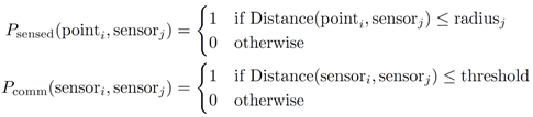 where and are the probabilities of the area point to be sensed by sensor node , and of the sensor nodes and to communicate respectively.
In this research work the Particle Swarm Optimization (PSO) methodology, which is a well-established metaheuristic method used extensively in practice in various fields, is adopted, in order to achieve the area coverage maximization [32,33].
The term particle refers to a possible solution to the problem, in our context the final optimal locations of sensor nodes. The term swarm refers to the set of all particles. As the execution of the algorithm progresses particles are essentially moving on the objective function range trying to find a possible solution. This particle movement is achieved through communication exchange of their current positions and a velocity update calculation according to the following equations:
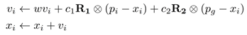 where denotes the velocity of the i-th particle, denotes the position of this particle, denotes the current best particle’s position, and is the best swarm position found till the current update. R1 and R2 are uniform random number vector generators, is the inertial weight, are the acceleration coefficients and ⨂ is the symbol of point-wise vector multiplication. The velocity update equation is comprised by three terms, which namely are the momentum term that attracts the solution towards the previous direction, the cognitive term that pushes the solution towards the personal best and the social term that attracts the solution close to the global best. An outline of a general PSO algorithm is illustrated in Figure 2.
2.2. Related Work
Coverage and connectivity problem optimization in WSNs keeps on being studied during all decades of the WSNs’ evolution [1,18,34]. Also, the field of metaheuristics in optimization, where PSO is categorized, is expanding for decades and includes dozens of methodology types and hundreds of their varieties [35]. Currently an enormous amount of research activity takes place around the world concerning the problems that arise in WSN deployment both in theoretical context and in practical application level. Some theoretical limits concerning coverage and connectivity in sensor networks can be found in [36].
A two-pass approach to the WSN coverage problem is given in [37] where first a PSO algorithm is used to deploy optimally the sensor nodes and at a second pass a Voronoi diagram method is employed to evaluate the solution fitness. In [38] the coverage of a square area is maximized using two approaches, one based on Genetic Algorithms (GA) and one on PSO. In both approaches the fitness function was chosen to be the area of the unmonitored part of the target region.
Tossa et al. in [39] introduces a Genetic Algorithm for Area Coverage Maximization (GAFACM) which works for both regular and irregular areas, with a predefined number of sensor nodes while guaranteeing their connectivity. An improved social spider optimization (SSO) algorithm is proposed in [40] where its global convergence speed is improved through a population initialization method based on chaos theory and by improving the neighborhood search, global search, and matching radius of the algorithm (Chaos SSO-CSSO).
An improved PSO that tackles possible local convergence problems is presented in [41], where the objective function incorporates coverage and distance metrics and the velocity update equation is augmented by a gravitational and a Coulomb term. A similar approach is presented in [42] where a virtual force-directed PSO (VFPSO) algorithm is employed to achieve maximal coverage. A more involved velocity update PSO equation is presented in [43] with the introduction of the Virtual Force Individual Particle Optimization VFIPO algorithm which is a combination of a Virtual Force (VF) algorithm, an Individual Particle Optimization (IPO) algorithm and a VFPSO variant. A Distributed Virtual Forces sensor redeployment Algorithm (DVFA) that does not require sensor node synchronization is presented in [44]. The algorithm redeploys an initially randomly deployed swarm of sensor nodes in such a way as to ensure the uniform coverage of the designated area and the connectivity of the network.
A Genetic Algorithm for area maximization, called MIGA, is proposed in [45]. It uses a novel heuristic initialization procedure, a new fitness function based on an exact integral area calculation and a combinatorial approach on the usage of the crossover operators. A Virtual Force Algorithm (VFA) is employed at the final stage to refine the final solution quality.
Du in [46] proposes the usage of a Virtual Force Algorithm (VFA), in combination with a distributed PSO variant (DPSO), for the solution of the 3D coverage of a designated spatial volume by 3D sensing sensor nodes while retaining connectivity. A fusion of various algorithms is presented in [47] where a Resampling Particle Swarm Optimization (RPSO) algorithm is combined with a Particle Swarm Optimization algorithm based on coefficient adjustment (PSO-D) and an improved Virtual Force (VF) algorithm. A method that combines chaos optimization theory and particle swarm optimization in [48] uses PSO first in order to move the sensor nodes close to their optimal positions and then a Variable Domain Chaos Optimization Algorithm (VDCOA) is employed in order to improve the coverage rate. In [49] a new hybrid algorithm (CFL-PSO) is introduced. It is based on combining an enhanced Fick’s Law (FL) algorithm (a diffusion type metaheuristic algorithm), with a Comprehensive Learning (CL) algorithm (another metaheuristic algorithm) and a Particle Swarm Optimization (PSO) algorithm, in order to achieve maximal area coverage and node connectivity by combining the strengths of all the aforementioned metaheuristic methodologies.
3. Proposed Methodology
3.1. PSO Algorithm Implementation
The approach used in the implementation of the PSO algorithm is based on [33]. The sense areas and the communication range patterns of the sensor nodes are considered circles of given radii. The main data structures which hold the required information of the particle swarm optimizer are:
- an array where each row corresponds to one of the particles and each column corresponds to one of the sensor nodes in that particle. The particles are considered vectors of the form , where each pair corresponds to the position of the th sensor node.
- an array which, similarly to the structure of the positions array, holds the n vectors of the velocity components of the sensor nodes of each particle
- an array which holds each particle’s personal best position vectors.
- an -element vector which holds each particle’s personal best objective function value.
- a variable containing the objective function value of the leader (global best) particle.
- a -element vector which holds the leader particle sensor node positions.
There are also several variables that hold the optimization parameters. These include the vectors holding the sensor nodes’ communication and sense ranges. The vectors containing the region of interest geometry. The structure that contains the number of particles, the number of sensor nodes, the value of the inertia weight , the values of the two acceleration coefficients , the parameter values of the objective function (see 3.2), the values of the velocity bounds (the same for both axes), the values of the maximum optimization iterations , the values of the two convergence parameters: stagnation iteration limit and percentage of change (i.e. convergence is achieved if the objective function value stays inside an band for iterations) and the value of the border bound percentage , where 100% denotes that the bounds on the allowed sensor node positions are the same with the region of interest borders. The last parameter is usually used to avoid small unmonitored areas at the borders if the combined sense area of all the sensor nodes exceeds the area to be covered. All spatial quantities are normalized.
The particle positions and velocities are initially randomized. In order to assess the performance of our algorithm, that is how much of the region of interest is covered by the sensor nodes, a Monte Carlo type estimation algorithm is used. A predetermined number of random points in the region are generated and they are checked whether they fall inside the sensing range of any of the sensor nodes. If they do, they are considered to be covered. The ratio of the number of covered points to the total number of generated points gives the estimate of the covered area. The more generated random points the greater the accuracy of the estimation but at the expense of more computation time. An outline of the PSO implementation is shown in Figure 3.
3.2. Objective Fitness Function
In [38] the optimization fitness function used for the PSO algorithm, concerned the direct covered area measurement. In this work, the proposed objective function metric stems from the field of discrete geometry optimization and especially that of finding the densest packing of similar objects in a bounded two-dimensional space.
The main idea involves treating the sense areas of the sensor nodes as circles of the same or different radii, an approximation usually done in practice, so as to approximate the WSN coverage problem with that of the dense packing of circles inside a given square, a well-studied discrete geometry problem. The problem of packing circles in a square can be expressed as follows [50]:
Problem statement.Locate n points in a unit square, such that the minimum distance dij between any two points i, j is maximal.
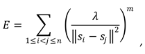
This problem can be expressed as a global optimization problem of the form:
An approach to find an approximate solution to the above problem is by utilizing that:
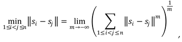
In this way the initial optimization in (3) transforms into:
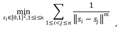 where and denote the position vectors of the centers of two circles and the Euclidean distance between them. The objective function in (5) resembles an energy function so the whole problem is similar to an energy minimization of repulsing electric charges distributed spatially, with the charges situated at the circles’ centers.
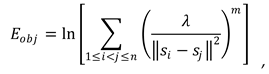
A similar energy function that incorporates a scaling factor and an exponent in the inverse-power interaction was proposed in [51]:
 The scaling factor adjusts for numerical stability when the distance between the sensor nodes is small, while the exponent regulates how strongly the interaction diminishes as sensor node distance increases and it is used as an additional adjustment factor in the optimization process.
In order to smooth out and improve numerical stability when encountering very large or very small numbers a logarithmic transformation is used. In this way, the optimization fitness function used becomes:
3.3. k-Coverage Implementation Algorithm
In order to achieve the desired k-coverage in some of the specified points in the sensed area the initial positions of k of each particle’s sensor nodes are assigned to the position of each of the specified points which require coverage from k sensor nodes. At each optimization iteration, a check whether the distances of the assigned sensor nodes from the k-covered points exceed the nodes’ radii is performed. If this happens their distance is bounded to that of their corresponding sense radius. The assigned sensor node’s bounded coordinates are calculated to be on the line connecting the specified k-covered point with the assigned node as shown in Figure 3. The previous bound checks are performed for all pairs of k-covered points and their assigned k nodes.
In Figure 4, point A is the specified k-covered point, point B is one of its assigned sensor nodes. The circle’s radius corresponds to the sense area radius R of that node. Point C is the intersection of their distance direction line with the sense area circle. The coordinates of C are the new bounded coordinates of the assigned node as its Euclidean distance d from the k-covered point exceeds that of the sense radius R and its coordinates are calculated as follows:
It is equivalent to center the sense circle in A although it should be centered in B in order to calculate the bounded coordinates towards B. This way the assigned nodes will always cover their respective k-covered points and maximize their mutual non overlapping coverage area.
When the sensor nodes in the WSN have different sense radii, they are assigned to their corresponding k-covered points in ascending sense radius order in order to leave the larger sense radius nodes flexibility to cover larger parts of the area of interest. It is also more beneficial when the k-covered points of interest lie close to the area border where larger sense radii assigned nodes will have greater possibility to have more mutually overlapped covered areas. In Figure 5, the k-coverage implementation algorithm is illustrated.
3.4 1-Connectivity Implementation Algorithm
The communication range pattern of each sensor node is considered circular with a radius double of that of their sensing range in case where two nodes have the same sense ranges. If two nodes have different sense ranges then their communication range should be equal to the sum of their respective sense ranges. In order for the sensor nodes to achieve the largest possible covered area, the communication range of each node should be chosen so that it is equal to the sum of its sensing range with the sensing range of the node with the largest sense range. This way a set of nodes of different sense radii could cover the maximal area with their sensor nodes while making it possible to maintain 1-connectivity (see examples in Figure 6).
To test the 1-connectivity of the sensor network a depth-first search (DFS) algorithm [52] is used on its distance weighted graph in order to identify the non-connected sensor nodes with the given sensor node communication ranges. In the PSO initialization phase, it is ensured that the initial random particle sensor node distributions are 1-connected. To achieve this the sensor nodes’ communication to sensing range ratios should be chosen according to the method stated previously. If this is not the case, the algorithm will abort after some predetermined number of tries if 1-connectivity is not achieved. In order to keep the sensor network 1-connected during the optimization process, each particle is checked for at least 1-connectivity for all optimization iterations. If at some iteration a particle’s spatial sensor node distribution checks that it is not at least 1-connected then it is maintained at its most recent 1-connected configuration. This continues till the convergence of the optimization process is achieved and ensures that the final optimal sensor node distribution will be at least 1-connected. The 1-connectivity constrain is executed after the k-coverage constrain (see 3.3) in the PSO process.
In Figure 7 the 1-connectivity implementation algorithm is illustrated.
4. Simulation Tests and Performance Evaluation
Performance evaluation of the proposed algorithm was conducted via simulations in the MathWorks MATLAB environment and through comparative analysis with seven test cases outlined in [37,38].
Because the PSO methodology is a probabilistic (stochastic) method, in each case study the simulation test was conducted 30 times. The mean value and the standard deviation of area coverage percentage were calculated and are presented in the corresponding tables. Additionally, the highest area coverage achieved in each case is included as well as the ideal coverage which is the combined coverage that all the sensor nodes can provide in an unbounded environment.
In each of the case studies analyzed, a comparative assessment of the investigated PSO algorithms was performed using t-test methodology. This statistical technique allows for the evaluation of hypotheses related to a population by determining the p-value, which quantifies the degree of agreement between the data and the null hypothesis. The null hypothesis, in this scenario, assumes that there is no difference in the mean results produced by the two competing algorithms. The statistical tests compared the proposed algorithm against the PSO algorithms and not the Genetic Algorithms.
The PSO parameters used have fixed values during the whole simulation. Their values were calculated through meta-optimization around an initial parameter vector on the first test case and then manually rounded off and tuned around these calculated values for each case [53]. The optimization method used was a direct search method based on a pattern search strategy which is an algorithm designed to solve nonlinear optimization problems without requiring gradient information [54,55]. The whole test case was entered as a function to the pattern search optimizer with the particle swarm parameters as the optimization variables. The particle swarm parameters used in the pattern search optimizer where the value of the inertia weight, the values of the two acceleration coefficients, the two parameter values of the objective function (see 3.2) and the values of the velocity bounds. All other parameters (particle number, maximum iterations, optimization termination tolerance) were chosen as close as possible to the respective values used in [38] in order to better compare the performance of the algorithms.
In all the case studies examined, the simulation results and the optimal node placement are depicted in the accompanying tables and figures. Specifically, in the figures depicting the optimal node locations with 1-connectivity, the cyan disks show the sense area of each node, the green circles the communication range of each node, the red lines show the established communication connections between the nodes and the numbers above the sensor node positions show with how many other nodes this sensor node is connected.
4.1. Case Study 1
In this case study, the primary objective was to maximize the coverage of a two-dimensional square area measuring 20 × 20 units. A total of 35 sensor nodes were deployed, each equipped with a sensing range of 1.5 units and a communication range of 3.0 units. The Particle Swarm Optimization (PSO) algorithm was configured with a particles size of 200 in the scenario with no connectivity required and 600 particles in the scenario requiring the 1-connectivity constrain.
The PSO parameters in the no connectivity requirement case were: =0.2, =1.5, =1.5, =0.7, =10, =0.05, =130, =20, =1%, =100%, while in the 1-connectivity requirement were: =0.2, =1.5, =1.5, =0.7, =10, =0.005, =130, =40, =1%, =100%.
In Table 1, the results of the corresponding simulation tests are shown. Both algorithms with and without 1-connectivity requirements had better area coverage percentage mean values and standard deviations than the Genetic Algorithm (GA) based and PSO based ones in [38] and were close to the ideal coverage. The p-value in the PSO with no connectivity requirement was negligible signifying that the proposed algorithm is better. In Figure 8 and Figure 9, the optimal node locations with and without 1-connectivity requirements are correspondingly shown. In Figure 10 the objective function value iterations for both requirements are illustrated.
4.2. Case Study 2
In this case study, the primary objective was to maximize the coverage of a two-dimensional square area measuring 20 × 20 units. A total of 32 sensor nodes were deployed with varying sense ranges. Five sensor nodes had a sensing range of 0.8 units and of a communication range 2.8 units. Twenty sensor nodes had a sensing range of 1.5 units and a communication range of3.5 units. Seven sensor nodes had a sensing range of 2 units and a communication range of4 units. The Particle Swarm Optimization (PSO) algorithm was configured with a particles size of 200 in the scenario with no connectivity required and 600 particles in the scenario requiring the 1-connectivity constrain.
The PSO parameters in the no connectivity requirement case were: =0.5, =1.5, =1.5, =0.7, =10, =0.01, =130, =20, =1%, =100%, while in the 1-connectivity requirement were: =0.2, =1.5, =1.5, =0.7, =10, =0.075, =130, =40, =1%, =100%.
In Table 2, the results of the corresponding simulation tests are shown. The algorithm without the 1-connectivity requirement had better area coverage percentage mean values and standard deviations than the PSO based one in [38] and was close to the ideal coverage. The p-value in the PSO with no connectivity requirement was negligible signifying that the proposed algorithm is better. In Figure 11 and Figure 12, the optimal node locations with and without 1-connectivity requirements are correspondingly shown. In Figure 13 the objective function value iterations for both requirements are illustrated.
4.3. Case Study 3
In this case study, the primary objective was to maximize the coverage of a two-dimensional square area measuring 20 × 20 units. A total of 45 sensor nodes were deployed, each equipped with a sensing range of 1.5 units and a communication range of 3.0 units. Additionally, it was required to have a 3-coverage constrain for 6 area points at positions (5, 5), (10, 5), (15, 5), (5, 15), (10, 15) and (15, 15).
The Particle Swarm Optimization (PSO) algorithm was configured with a particles size of 600 in the scenario with no connectivity required and 1200 particles in the scenario requiring the 1-connectivity constrain.
The PSO parameters in the no connectivity requirement case were: =0.2, =1.5, =1.5, =0.7, =10, =1.0, =130, =20, =1%, =100%, while in the 1-connectivity requirement were: =0.2, =1.5, =1.5, =0.7, =10, =0.2, =130, =40, =1%, =100%.
In Table 3, the results of the corresponding simulation tests are shown. Both algorithms with and without 1-connectivity requirements had better area coverage percentage mean values than the PSO based one in [38] and the 3-coverage constrain was satisfied on all required points. The p-value in the PSO with no connectivity requirement was negligible signifying that the proposed algorithm is better. In Figure 14 and Figure 15, the optimal node locations with and without 1-connectivity requirements are correspondingly shown. In Figure 16 the objective function value iterations for both requirements are illustrated.
4.4. Case Study 4
In this case study, the primary objective was to maximize the coverage of a two-dimensional square area measuring 20 × 20 units. A total of 45 sensor nodes were deployed this time with varying sense ranges. Eighteen sensor nodes had a 1.0 unit sensing range and a communication range of 3.0 units. Twenty sensor nodes had a sensing range of 1.5 units and a communication range of 3.5 units. Seven sensor nodes had a sensing range of 2 units and a communication range of 4 units. Also, it was required to have a 3-coverage constrain for 6 area points at positions (5, 5), (10, 5), (15, 5), (5, 15), (10, 15) and (15, 15).
The Particle Swarm Optimization (PSO) algorithm was configured with a particles size of 600 in the scenario with no connectivity required and 1200 particles in the scenario requiring the 1-connectivity constrain.
The PSO parameters in the no connectivity requirement case were: =0.47, =1.59, =1.53, =0.24, =3.15, =1.75, =240, =100, =0.01%, =100%, while in the 1-connectivity requirement were: =0.5, =1.56, =1.56, =0.24, =3, =0.05, =240, =40, =1%, =100%.
In Table 4, the results of the relevant simulation tests are shown. The PSO algorithm without the 1-connectivity requirement has slightly better area coverage percentage mean value than the GA based one in [38] while the 3-coverage constrain is satisfied on all required points. The p-value between the proposed PSO with no connectivity requirement algorithm and the GA based one in [38] is 0.066 signifying that there is some evidence that the proposed algorithm is better in this case. Although this test case is computationally expensive due to its complexity, further tuning of the PSO algorithm’s parameters is feasible and will further increase its performance. In Figure 17 and Figure 18, the optimal node locations with and without 1-connectivity requirements are respectively shown. In Figure 19 the objective function value iterations for both requirements are shown.
4.5. Case Study 5
In this case study, the primary objective was to maximize the coverage of a two-dimensional square area measuring 50 × 50 units. A total of 40 sensor nodes were deployed, each equipped with a sensing range of 5.0 units and a communication range of 10.0 units. The Particle Swarm Optimization (PSO) algorithm was configured with a particles size of 200 for both the scenarios with no connectivity required and the scenario requiring the 1-connectivity constrain.
The PSO parameters in the no connectivity requirement case were: =0.5, =1.5, =1.5, =0.2133, =3, =1.0, =200, =200, =1%, =100%, while in the 1-connectivity requirement were: =0.5, =1.5, =1.5, =0.2133, =3, =0.02, =250, =250, =1%, =100%. In this case there was no convergence limit and the border bound percentage was set in such a way as to allow the sensor nodes to move closer to the area boundary and leave no unmonitored parts at the border as the combined sense area of the sensor nodes exceeds the total target area.
In Table 5, the results of the corresponding simulation tests are shown. Both algorithms with and without 1-connectivity requirements had better area coverage percentage mean values and standard deviations than the Genetic Algorithm (GA) based and PSO based ones in [38] and were quite close to the ideal coverage. The p-value in the PSO with no connectivity requirement was negligible signifying that the proposed algorithm is better. In Figure 20 and Figure 21, the optimal node locations with and without 1-connectivity requirements are correspondingly shown. In Figure 22 the objective function value iterations for both requirements are illustrated.
4.6. Case Study 6
In this case study, the primary objective was to maximize the coverage of a two-dimensional square area measuring 50 × 50 units. A total of 20 sensor nodes were deployed, each equipped with a sensing range of 5.0 units and a communication range of 10.0 units. The Particle Swarm Optimization (PSO) algorithm was configured with a particles size of 200 for both the scenario with no connectivity required and the scenario requiring the 1-connectivity constrain.
The PSO parameters in the no connectivity requirement case were: =0.5, =1.5, =1.5, =0.2133, =3, =0.16, =150, =150, =1%, =100%, while in the 1-connectivity requirement were: =0.5, =1.5, =1.5, =0.2133, =3, =0.016, =200, =200, =1%, =100%. In this case there was no convergence limit.
In Table 6, the results of the corresponding simulation tests are shown. The algorithm without the 1-connectivity requirement had better area coverage percentage mean value and standard deviation than the Genetic Algorithm (GA) based and PSO based ones in [38] and were close to the ideal coverage. The p-value in the PSO with no connectivity requirement was negligible signifying that the proposed algorithm is better. In Figure 23 and Figure 24, the optimal node locations with and without 1-connectivity requirements are correspondingly shown. In Figure 25 the objective function value iterations for both requirements are illustrated.
4.7. Case Study 7
In this case study, the primary objective was to maximize the coverage of a two-dimensional square area measuring 30 × 30 units. A total of 20 sensor nodes were deployed, each equipped with a sensing range of 5.0 units and a communication range of 10.0 units. The Particle Swarm Optimization (PSO) algorithm was configured with a particles size of 50 for both the scenario with no connectivity required and the scenario requiring the 1-connectivity constrain.
The PSO parameters in the no connectivity requirement case were: =0.4, =1.5, =1.575, =0.3, =1.5, =16.67, =1000, =1000, =1%, =100%, while in the 1-connectivity requirement were: =0.4, =1.5, =1.575, =0.3, =1.5, =16.67, =500, =500, =1%, =100%. In this case there was no convergence limit and the border bound percentage was set in such a way as to allow the sensor nodes to move closer to the area boundary and leave no unmonitored parts at the border as the combined sense area of the sensor nodes exceeds the total target area.
In Table 7, the results of the corresponding simulation tests are shown. Both algorithms with and without 1-connectivity requirements had better area coverage percentage mean values and standard deviations than the Genetic Algorithm (GA) based and PSO based ones in [38] and were quite close to the ideal coverage. The p-value in the PSO with no connectivity requirement was negligible signifying that the proposed algorithm is better. In Figure 26 and Figure 27, the optimal node locations with and without 1-connectivity requirements are correspondingly shown. In Figure 28 the objective function value iterations for both requirements are illustrated.
5. Conclusions and Future Work
In this paper, a novel Particle Swarm Optimization (PSO) approach tackling the problem of the optimal placement of a predefined number of sensor nodes within a square target area, adhering to k-coverage and 1-connectivity constraints is proposed. Also, a new objective function derived from circle packing geometric problems is introduced. This function serves as an alternative to traditional area coverage minimization objectives and simplifies implementation. The objective function resembles the repulsion force-based methods but with a much cleaner definition and simpler implementation.
We tested our method against seven benchmark test cases presented in [38]. Two of the test cases included 3-coverage constrain of 6 predefined points in the region and two test cases required different sensing and communication ranges of the sensor nodes. Each test case was executed 30 times and involved the computation of the mean and standard deviation of the area coverage percentage, thereby accounting for the stochastic nature of the PSO algorithm.
Our findings indicate that in six out of the seven test cases, our PSO method was better in terms of either or both the mean value and the standard deviation of the area coverage percentage. The statistical significance of this was confirmed using the t-test methodology. In one test case involving the 3-coverage of six points of interest, our methodology demonstrated better performance compared to the Genetic Algorithm-based approach used in [38]. This test case is quite challenging and computationally intensive especially with the 1-connectivity constrain. It is anticipated that further tuning of the PSO parameters and/or change of the PSO implementation methodology—such as using a variable inertia weight or adjusting other PSO parameters across algorithm iterations, or selecting a different static or dynamic population topology—could enhance its performance.
The presented methodology showed promising results and could be generalized and extended in various different aspects in the future like those presented in the following paragraphs.
Extension to arbitrary target areas, i.e. generalize and test our method on various geometric shapes beyond square regions, adapting the algorithm to handle irregular boundaries or even obstacles within the deployment area.
Generalization of sensor node sensing patterns, i.e. make changes to accommodate for diverse sensor node sensing patterns, not limited to circular ones. This could be achieved by incorporating directional parameters into the objective function thus making possible the modeling of anisotropic sensing fields which is common in practical WSN applications.
General communication radiation patterns, i.e. extending our method to handle realistic, non-circular communication range patterns. This could be achieved by employing Laplacian eigenvalue methodologies used extensively in robotics [56,57] instead of the direct search methods used in this work. This could also facilitate the incorporation of m-connectivity constraints thus improving network robustness and fault tolerance.
Application in other metaheuristics, i.e. to investigate the effectiveness of our proposed objective function within other metaheuristic optimization frameworks, except the PSO method.
Minimal Sensor Deployment, i.e. to adapt our method to not only maximize coverage but also to determine the minimal number of sensor nodes required for a given coverage and connectivity application. This could have significant implications in cost reduction and resource efficiency.
Energy consumption modeling, i.e. to try to integrate energy models into our optimization framework, as energy efficiency directly impacts network lifespan.
Robustness against failures, i.e. to assess the resilience of our deployment strategy under varying environmental conditions and node failures and incorporate dynamic adaptation mechanisms to enhance its performance.
Finally, the validation of our method through real-world deployments is crucial to assess the practical feasibility and performance of our approach in operational environments.
Author Contributions
Conceptualization, G.S. and D.K.; methodology, G.S. and D.K.; software, G.S.; validation, G.S. and D.K.; formal analysis, G.S.; investigation, G.S. and D.K.; resources, G.S. and D.K.; data curation, G.S. and D.K.; writing—original draft preparation, G.S.; writing—review and editing G.S. and D.K.; visualization, G.S. and D.K.; supervision, D.K.; project administration, G.S. and D.K. All authors have read and agreed to the published version of the manuscript.
Funding
This research received no external funding.
Conflicts of Interest
The authors declare no conflicts of interest.
References
- Akyildiz, I.F.; Su, W.; Sankarasubramaniam, Y.; Cayirci, E. Wireless Sensor Networks: A Survey. Comput. Netw. 2002, 38, 393–422. [Google Scholar] [CrossRef]
- Yick, J.; Mukherjee, B.; Ghosal, D. Wireless Sensor Network Survey. Comput. Netw. 2008, 52, 2292–2330. [Google Scholar] [CrossRef]
- Kandris, D.; Nakas, C.; Vomvas, D.; Koulouras, G. Applications of Wireless Sensor Networks: An Up-To-Date Survey. Appl. Syst. Innov. 2020, 3, 14. [Google Scholar] [CrossRef]
- Sunehra, D.; Rajasri, S. Automatic Street Light Control System Using Wireless Sensor Networks. 2017 IEEE International Conference on Power, Control, Signals and Instrumentation Engineering (ICPCSI), 2017. [Google Scholar] [CrossRef]
- Papadakis, N.; Koukoulas, N.; Christakis, I.; Stavrakas, I.; Kandris, D. An IoT-Based Participatory Antitheft System for Public Safety Enhancement in Smart Cities. Smart Cities 2021, 4, 919–937. [Google Scholar] [CrossRef]
- Noel, A.; Abderrazak Abdaoui; Tarek Elfouly; Ahmed, M. H.; Badawy, A.; Shehata, M. Structural Health Monitoring Using Wireless Sensor Networks: A Comprehensive Survey. IEEE Communications Surveys and Tutorials 2017, 19, 1403–1423. [Google Scholar] [CrossRef]
- Orfanos, V. A.; Kaminaris, S. D.; Papageorgas, P.; Piromalis, D.; Kandris, D. A Comprehensive Review of IoT Networking Technologies for Smart Home Automation Applications. Journal of Sensor and Actuator Networks 2023, 12, 30. [Google Scholar] [CrossRef]
- Nikolidakis, S.A.; Kandris, D.; Vergados, D.D.; Douligeris, C. Energy efficient automated control of irrigation in agriculture by using wireless sensor networks. Comput. Electron. Agric. 2015, 113, 154–163. [Google Scholar] [CrossRef]
- Arshad, J.; Siddiqui, T. A.; Sheikh, M. I.; Waseem, M. S.; Nawaz, M. A. B.; Eldin, E. T.; Rehman, A. U. Deployment of an Intelligent and Secure Cattle Health Monitoring System. Egyptian Informatics Journal 2023, 24, 265–275. [Google Scholar] [CrossRef]
- Jabeen, T.; Jabeen, I.; Ashraf, H.; Jhanjhi, N. Z.; Yassine, A.; Hossain, M. S. An Intelligent Healthcare System Using IoT in Wireless Sensor Network. Sensor nodes 2023, 23, 5055. [Google Scholar] [CrossRef]
- Majid, M.; Habib, S.; Javed, A. R.; Rizwan, M.; Srivastava, G.; Gadekallu, T. R.; Lin, J. C.-W. Applications of Wireless Sensor Networks and Internet of Things Frameworks in the Industry Revolution 4.0: A Systematic Literature Review. Sensor nodes 2022, 22, 2087. [Google Scholar] [CrossRef]
- Christakis, I.; Tsakiridis, O.; Kandris, D.; Stavrakas, I. Air Pollution Monitoring via Wireless Sensor Networks: The Investigation and Correction of the Aging Behavior of Electrochemical Gaseous Pollutant Sensor nodes. Electronics 2023, 12, 1842. [Google Scholar] [CrossRef]
- Pantazis, N.A.; Nikolidakis, S.A.; Kandris, D.; Vergados, D.D. An Automated System for Integrated Service Management in Emergency Situations. In Proceedings of the 2011 15th Panhellenic Conference on Informatics, Kastonia, Greece, 30 September-2 October 2011; pp. 154–157. [Google Scholar]
- Đurišić, M.P.; Tafa, Z.; Dimić, G.; Milutinović, V. A Survey of military applications of wireless sensor networks. In Proceedings of the 2012 Mediterranean Conference on Embedded Computing (MECO), Bar, Montenegro, 19–21 June 2012; pp. 196–199. [Google Scholar]
- Kandris, D.; Anastasiadis, E. Advanced Wireless Sensor Networks: Applications, Challenges and Research Trends. Electronics 2024, 13, 2268. [Google Scholar] [CrossRef]
- Kandris, D.; Alexandridis, A.; Dagiuklas, T.; Panaousis, E.; Vergados, D. D. Multiobjective Optimization Algorithms for Wireless Sensor Networks. Wireless Communications and Mobile Computing 2020, 2020, 1–5. [Google Scholar] [CrossRef]
- Al-Karaki, J.N.; Gawanmeh, A. The Optimal Deployment, Coverage, and Connectivity Problems in Wireless Sensor Networks: Revisited. IEEE Access 2017, 5, 18051–18065. [Google Scholar] [CrossRef]
- Tripathi, A.; Gupta, H.P.; Dutta, T.; Mishra, R.; Shukla, K.K.; Jit, S. Coverage and Connectivity in WSNs: A Survey, Research Issues and Challenges. IEEE Access 2018, 6, 26971–26992. [Google Scholar] [CrossRef]
- Farsi, M.; Elhosseini, M.A.; Badawy, M.; Arafat Ali, H.; Zain Eldin, H. Deployment Techniques in Wireless Sensor Networks, Coverage and Connectivity: A Survey. IEEE Access 2019, 7, 28940–28954. [Google Scholar] [CrossRef]
- Evangelakos, E.A.; Kandris, D.; Rountos, D.; Tselikis, G.; Anastasiadis, E. Energy Sustainability in Wireless Sensor Networks: An Analytical Survey. J. Low Power Electron. Appl. 2022, 12, 65. [Google Scholar] [CrossRef]
- Bohloulzadeh, A.; Rajaei, M. A Survey on Congestion Control Protocols in Wireless Sensor Networks. Int. J. Wirel. Inf. Netw. 2020. [Google Scholar] [CrossRef]
- Chiwariro, R.; Thangadurai, N. Quality of Service Aware Routing Protocols in Wireless Multimedia Sensor Networks: Survey. Int. J. Inf. Technol. 2020, 14, 789–800. [Google Scholar] [CrossRef]
- Yu, J.-Y.; Lee, E.; Oh, S.-R.; Seo, Y.-D.; Kim, Y.-G. A Survey on Security Requirements for WSNs: Focusing on the Characteristics Related to Security. IEEE Access 2020, 8, 45304–45324. [Google Scholar] [CrossRef]
- Randhawa, S.; Jain, S. Data Aggregation in Wireless Sensor Networks: Previous Research, Current Status and Future Directions. Wirel. Pers. Commun. 2017, 97, 3355–3425. [Google Scholar] [CrossRef]
- Adday, G.H.; Subramaniam, S.K.; Zukarnain, Z.A.; Samian, N. Fault Tolerance Structures in Wireless Sensor Networks (WSNs): Survey, Classification, and Future Directions. Sensor nodes 2022, 22, 6041. [Google Scholar] [CrossRef]
- Sneha, V.; Nagarajan, M. Localization in Wireless Sensor Networks: A Review. Cybern. Inf. Technol. 2020, 20, 3–26. [Google Scholar] [CrossRef]
- Yadav, J.; Mann, S. Coverage in wireless sensor networks: A survey. Int. J. Electron. Comput. Sci. Eng. 2013, 2, 465–471. [Google Scholar]
- Ammari, H. M. Coverage in Wireless Sensor Networks: A Survey. Network Protocols and Algorithms 2010, 2. [Google Scholar] [CrossRef]
- Mihaela Cardei. Coverage Problems in Sensor Networks. Springer eBooks 2013, 899–927. [Google Scholar] [CrossRef]
- Wang, Y.; Zhang, Y.; Liu, J.; Bhandari, R. Coverage, Connectivity, and Deployment in Wireless Sensor Networks. Signals and communication technology 2014, 25–44. [Google Scholar] [CrossRef]
- Wang, B. Coverage Control in Sensor Networks; Springer London: London, 2010. [Google Scholar] [CrossRef]
- Engelbrecht, A. P. Particle Swarm Optimization. In Computational Intelligence : An Introduction; John Wiley ; Chichester: Hoboken, N.J, 2007; pp. 289–358. [Google Scholar]
- Poli, R.; Kennedy, J.; Blackwell, T. Particle Swarm Optimization. Swarm Intelligence 2007, 1, 33–57. [Google Scholar] [CrossRef]
- Mason, A.; Yazdi, N.; Chavan, A. V.; Najafi, K.; Wise, K. D. A Generic Multielement Microsystem for Portable Wireless Applications. Proceedings of the IEEE 1998, 86, 1733–1746. [Google Scholar] [CrossRef]
- Ezugwu, A. E.; Shukla, A. K.; Nath, R.; Akinyelu, A. A.; Agushaka, J. O.; Chiroma, H.; Muhuri, P. K. Metaheuristics: A Comprehensive Overview and Classification along with Bibliometric Analysis. Artificial Intelligence Review 2021. [Google Scholar] [CrossRef]
- Brass, P. Geometric Problems on Coverage in Sensor Networks. Bolyai Society mathematical studies 2013, 91–108. [Google Scholar] [CrossRef]
- Nor Aziz; Ammar Mohemmed; Mohammad Haji Alias. A Wireless Sensor Network Coverage Optimization Algorithm Based on Particle Swarm Optimization and Voronoi Diagram. 2009. [CrossRef]
- Tarnaris, K.; Preka, I.; Kandris, D.; Alexandridis, A. Coverage and K-Coverage Optimization in Wireless Sensor Networks Using Computational Intelligence Methods: A Comparative Study. Electronics 2020, 9, 675. [Google Scholar] [CrossRef]
- Tossa, F. U.; Abdou, W.; Ansari, K.; Ezin, E. C.; Gouton, P. Area Coverage Maximization under Connectivity Constraint in Wireless Sensor Networks. 2022, 22, 1712–1712. [CrossRef]
- Cao, L.; Yue, Y.; Cai, Y.; Zhang, Y. A Novel Coverage Optimization Strategy for Heterogeneous Wireless Sensor Networks Based on Connectivity and Reliability. IEEE Access 2021, 9, 18424–18442. [Google Scholar] [CrossRef]
- Wang, Y.; Li, M. Coverage Control Optimization Algorithm for Wireless Sensor Networks Based on Combinatorial Mathematics. Mathematical Problems in Engineering 2021, 2021, 1–8. [Google Scholar] [CrossRef]
- Wang, X.; Wang, S.; Bi, D. Virtual Force-Directed Particle Swarm Optimization for Dynamic Deployment in Wireless Sensor Networks. Springer eBooks 2007, 292–303. [Google Scholar] [CrossRef]
- Dirafzoon, S. M. A. Salehizadeh, S. Emrani and M. B. Menhaj. Virtual Force Based Individual Particle Optimization for Coverage in Wireless Sensor Networks. CCECE 2010, Calgary, AB, Canada: 2010, 1-4. https, 2010. [Google Scholar] [CrossRef]
- Mougou, K.; Mahfoudh, S.; Minet, P.; Laouiti, A. Redeployment of Randomly Deployed Wireless Mobile Sensor Nodes. 2012 IEEE Vehicular Technology Conference (VTC Fall), 2012; 1–5. [Google Scholar] [CrossRef]
- Hanh, N. T.; Binh, H. T. T.; Hoai, N. X.; Palaniswami, M. S. An Efficient Genetic Algorithm for Maximizing Area Coverage in Wireless Sensor Networks. Information Sciences 2019, 488, 58–75. [Google Scholar] [CrossRef]
- Du, Y. Method for the Optimal Sensor Deployment of WSNs in 3D Terrain Based on the DPSOVF Algorithm. IEEE Access 2020, 8, 140806–140821. [Google Scholar] [CrossRef]
- Qi, X.; Li, Z.; Chen, C.; Liu, L. A Wireless Sensor Node Deployment Scheme Based on Embedded Virtual Force Resampling Particle Swarm Optimization Algorithm. Applied intelligence 2021, 52, 7420–7441. [Google Scholar] [CrossRef]
- Zhao, Q.; Li, C.; Zhu, D.; Xie, C. Coverage Optimization of Wireless Sensor Networks Using Combinations of PSO and Chaos Optimization. Electronics 2022, 11, 853. [Google Scholar] [CrossRef]
- Amer, D. A.; Soliman, S. A.; Hassan, A. F.; Zamel, A. A. Enhancing Connectivity and Coverage in Wireless Sensor Networks: A Hybrid Comprehensive Learning-Fick’s Algorithm with Particle Swarm Optimization for Router Node Placement. Neural Computing and Applications 2024. [Google Scholar] [CrossRef]
- Péter Gábor Szabó; Mihály Csaba Markót; Tibor Csendes. Global Optimization in Geometry — Circle Packing into the Square. Springer eBooks, 2005; 233–265. [CrossRef]
- Nurmela, K. J.; Östergård, P. R. J. Packing up to 50 Equal Circles in a Square. Discrete & Computational Geometry 1997, 18, 111–120. [Google Scholar] [CrossRef]
- Cormen, T. H. ; Charles Eric Leiserson; Rivest, R. L., Stein, C. Introduction to Algorithms, Eds.; The Mit Press: Cambridge, Massachusetts, 2022. [Google Scholar]
- Pedersen, M. E. H.; Chipperfield, A. J. Simplifying Particle Swarm Optimization. Applied Soft Computing 2010, 10, 618–628. [Google Scholar] [CrossRef]
- Kolda, T. G.; Lewis, R. M.; Torczon, V. Optimization by Direct Search: New Perspectives on Some Classical and Modern Methods. SIAM Review 2003, 45, 385–482. [Google Scholar] [CrossRef]
- Find minimum of function using pattern search - MATLAB patternsearch. www.mathworks.com. https://www.mathworks.com/help/gads/patternsearch.html (accessed on 28 10 2024). (accessed on 28 10 2024).
- Olfati-Saber, R.; Fax, J. A.; Murray, R. M. Consensus and Cooperation in Networked Multi-Agent Systems. Proceedings of the IEEE 2007, 95, 215–233. [Google Scholar] [CrossRef]
- Zavlanos, M. M.; Egerstedt, M. B.; Pappas, G. J. Graph-Theoretic Connectivity Control of Mobile Robot Networks. Proceedings of the IEEE 2011, 99, 1525–1540. [Google Scholar] [CrossRef]
Figure 1.
Architecture of a typical WSN.
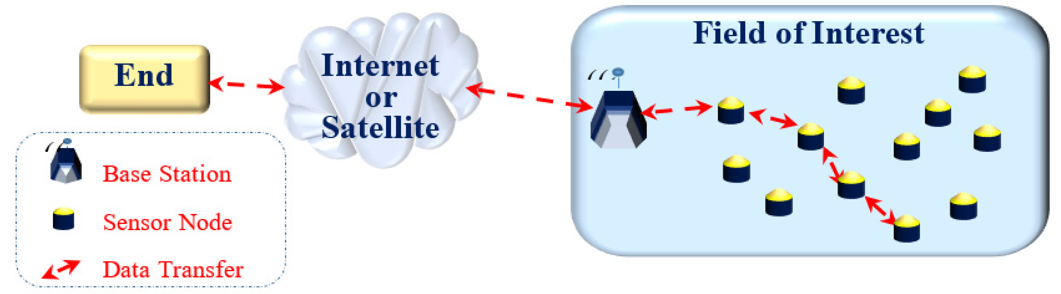
Figure 2.
General PSO algorithm outline.
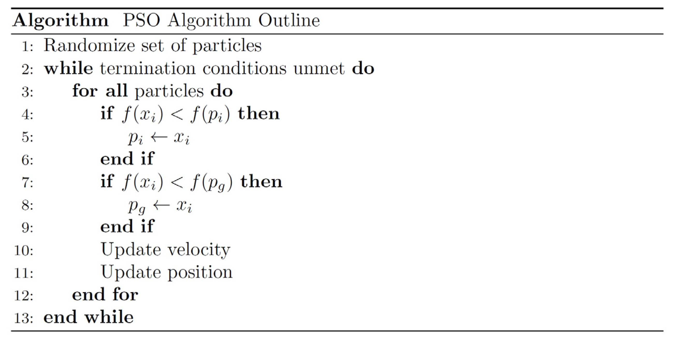
Figure 3.
PSO implementation algorithm.
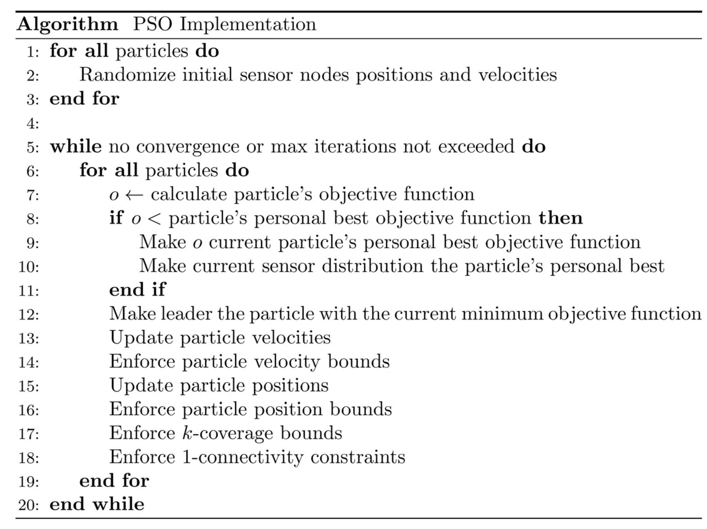
Figure 4.
k-Coverage sensor-point geometry.
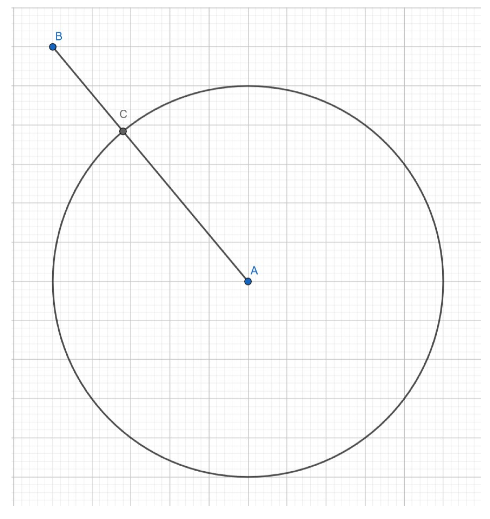
Figure 5.
k-Coverage implementation algorithm.
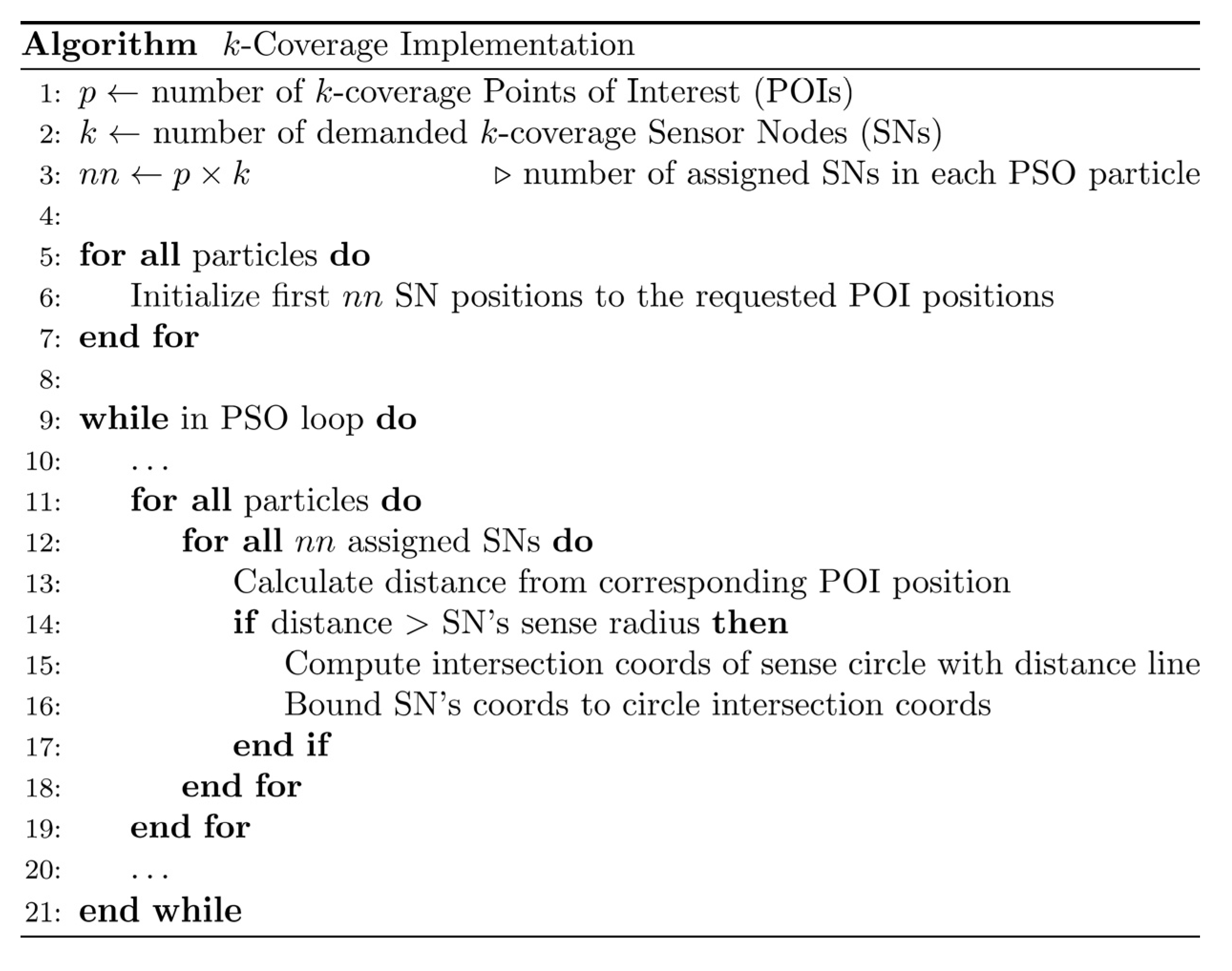
Figure 6.
Calculation example of two sensor nodes communication ranges (dashed lines) based on their sense ranges (solid lines) (a) both sense ranges = 3, communication ranges = 6; (b) sense ranges = 2 and 3, communication ranges = 5.
Figure 6.
Calculation example of two sensor nodes communication ranges (dashed lines) based on their sense ranges (solid lines) (a) both sense ranges = 3, communication ranges = 6; (b) sense ranges = 2 and 3, communication ranges = 5.
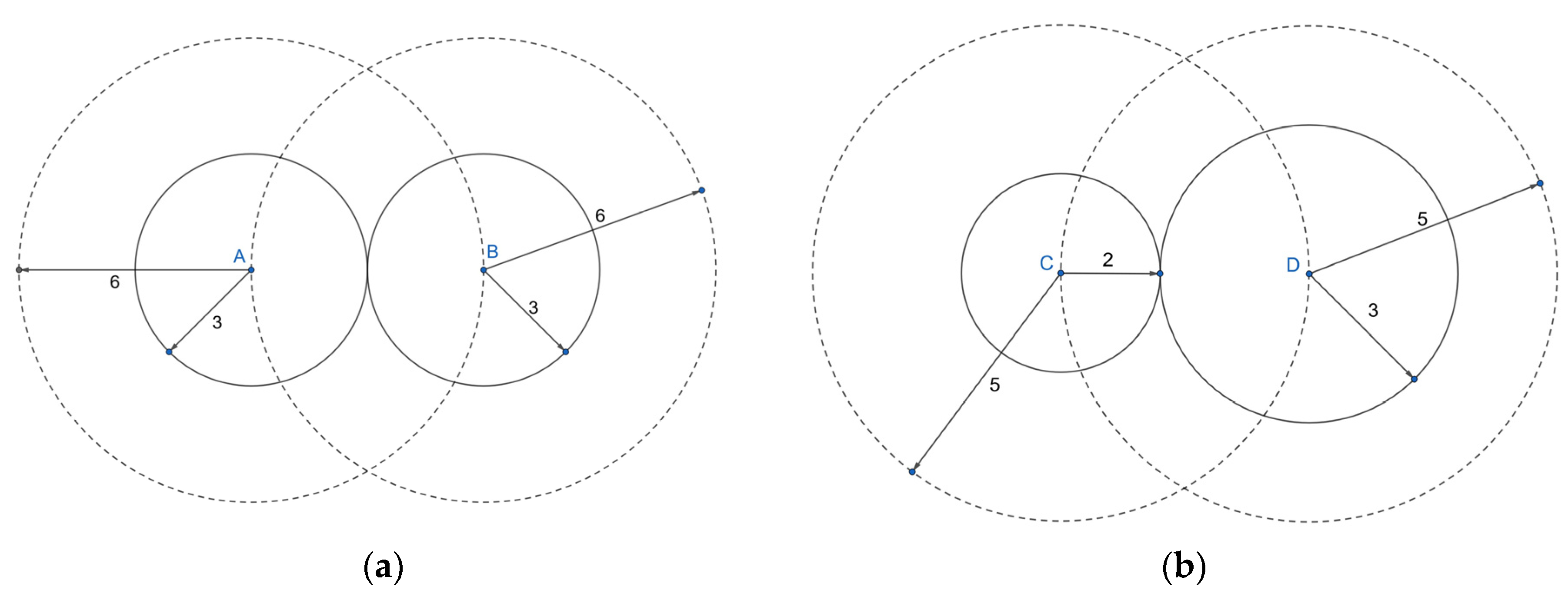
Figure 7.
1-Connectivity implementation algorithm.
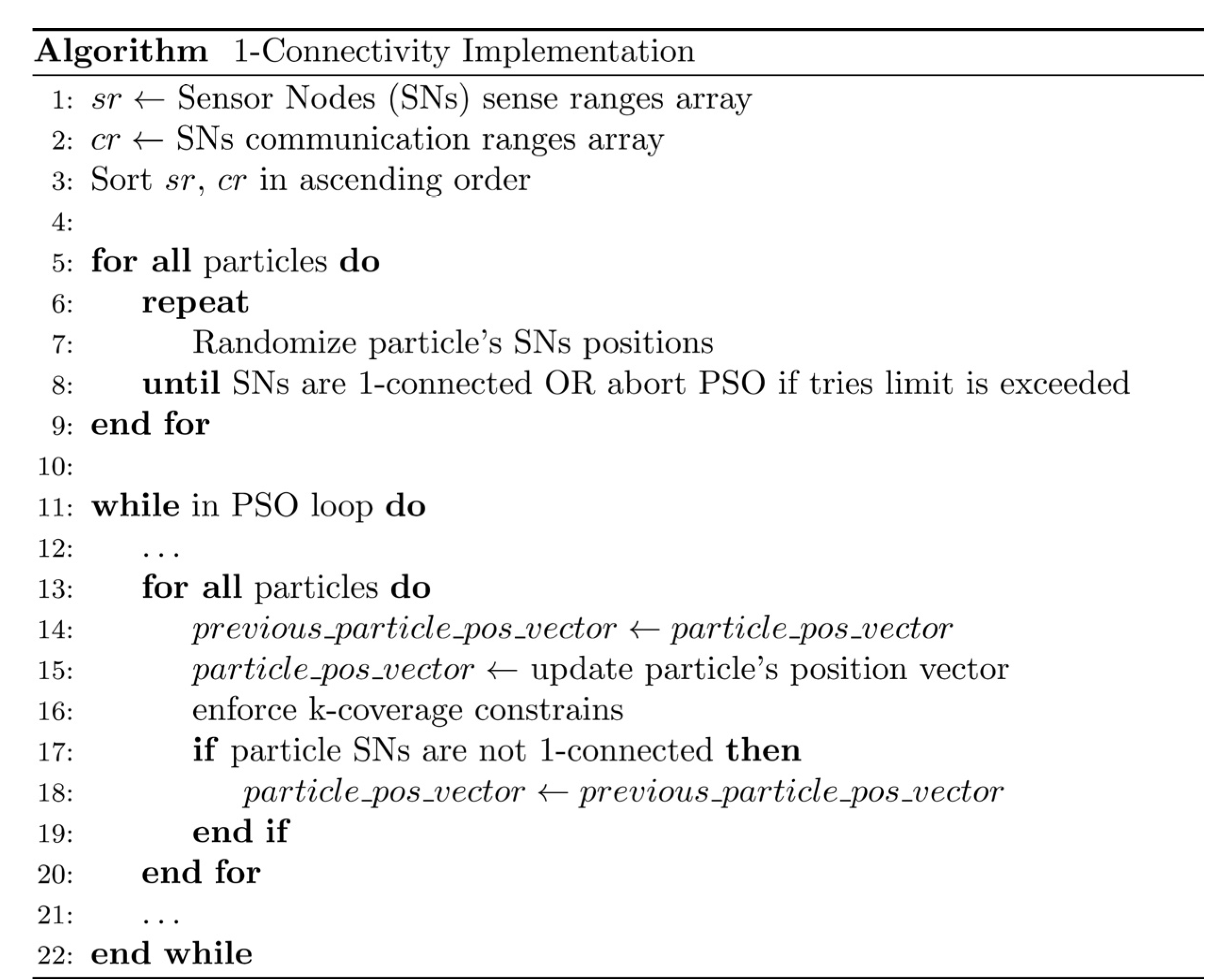
Figure 8.
Case study 1: Optimal node locations.
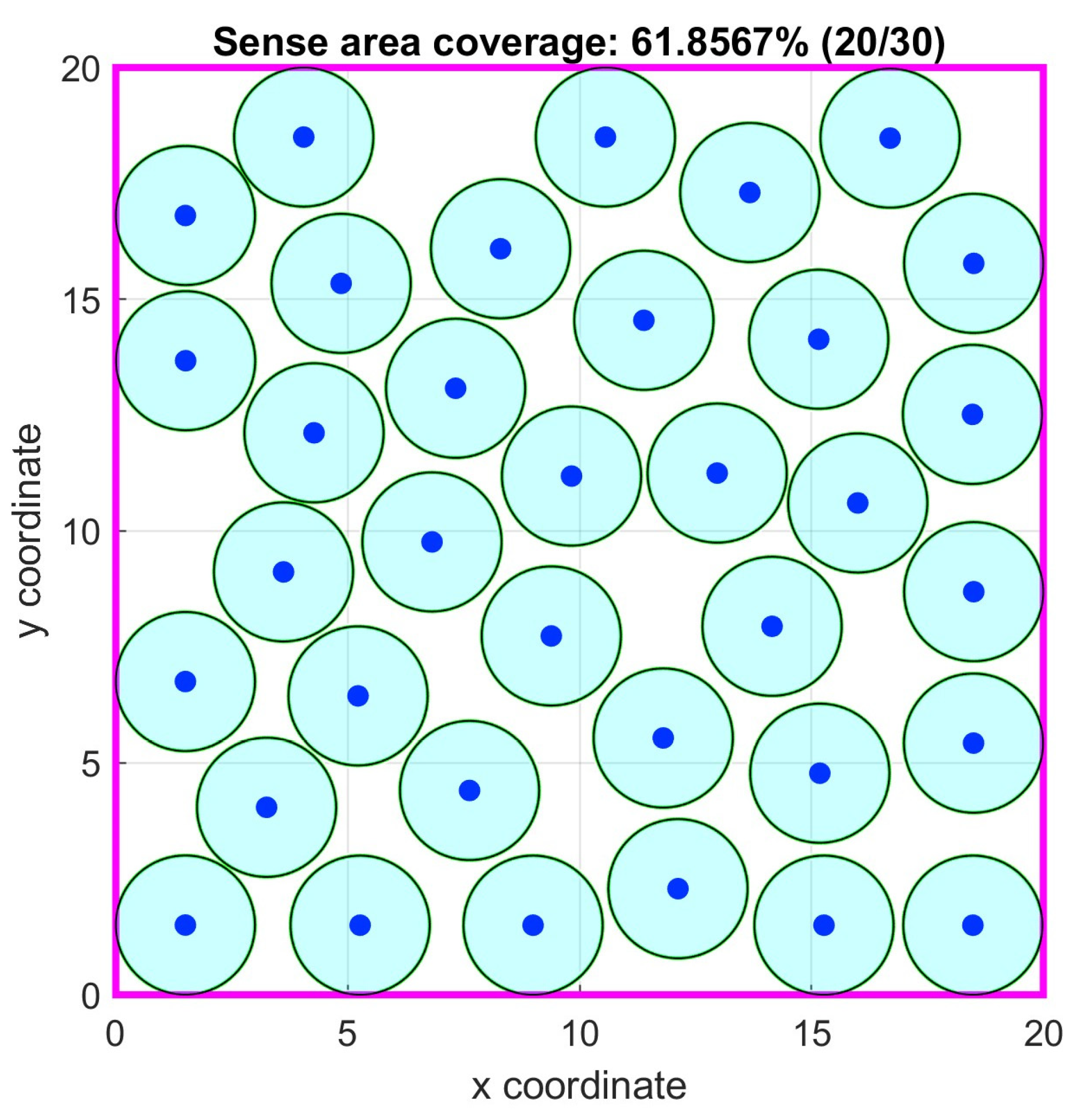
Figure 9.
Case study 1: Optimal node locations with 1-connectivity.
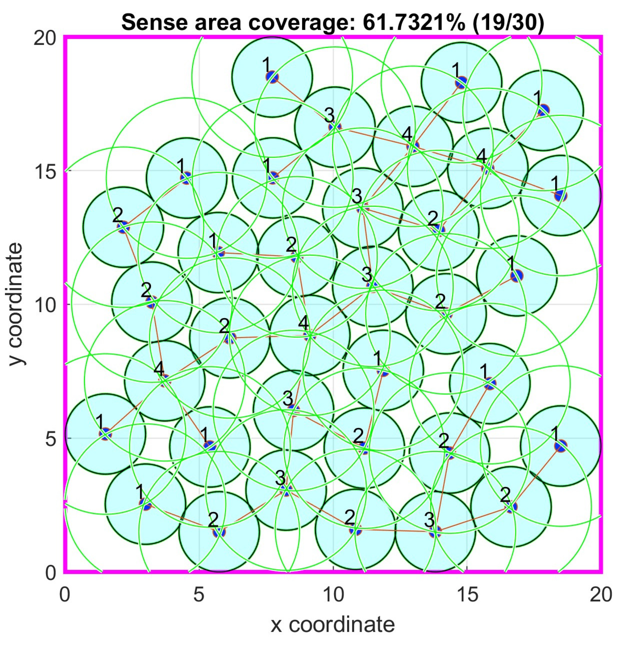
Figure 10.
Case study 1: Objective function iterations (a) No connectivity; (b) 1-connectivity.
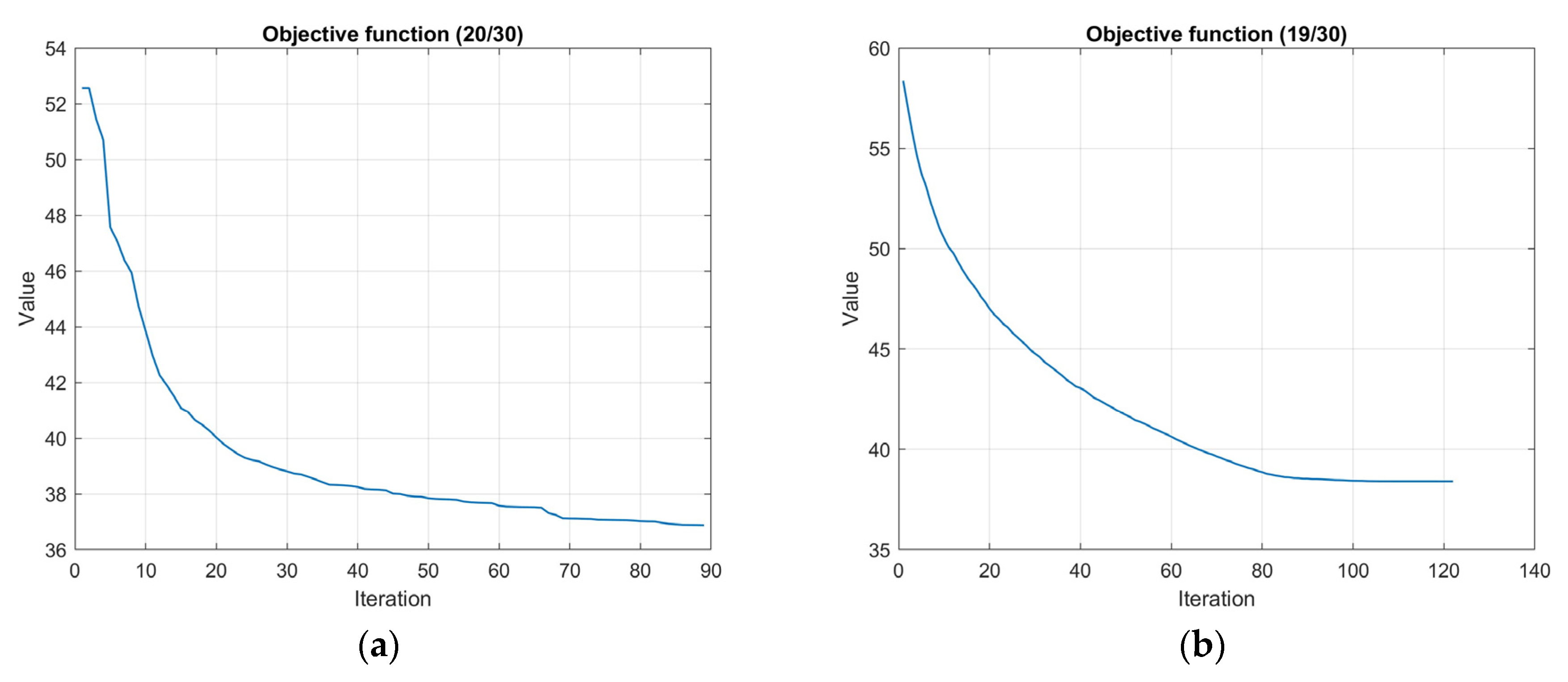
Figure 11.
Case study 2: Optimal node locations.
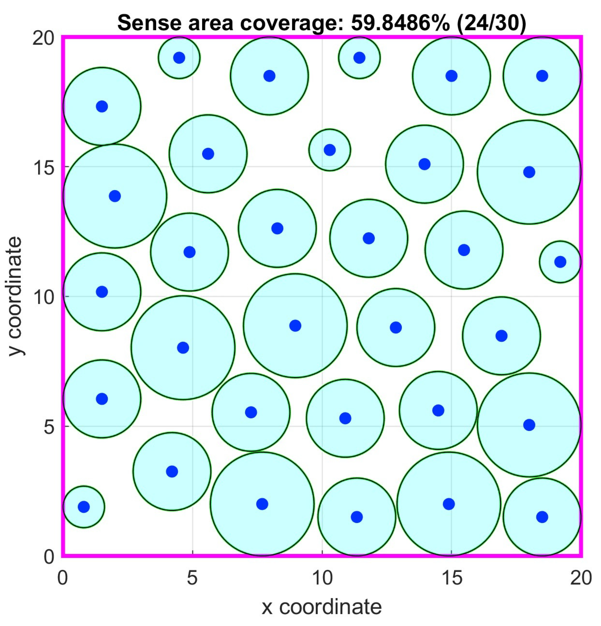
Figure 12.
Case study 2: Optimal node locations with 1-connectivity.
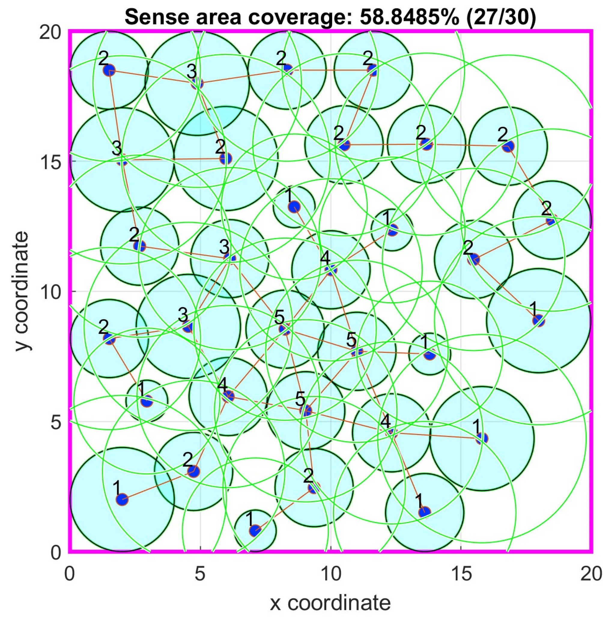
Figure 13.
Case study 2: Objective function iterations (a) No connectivity; (b) 1-connectivity.
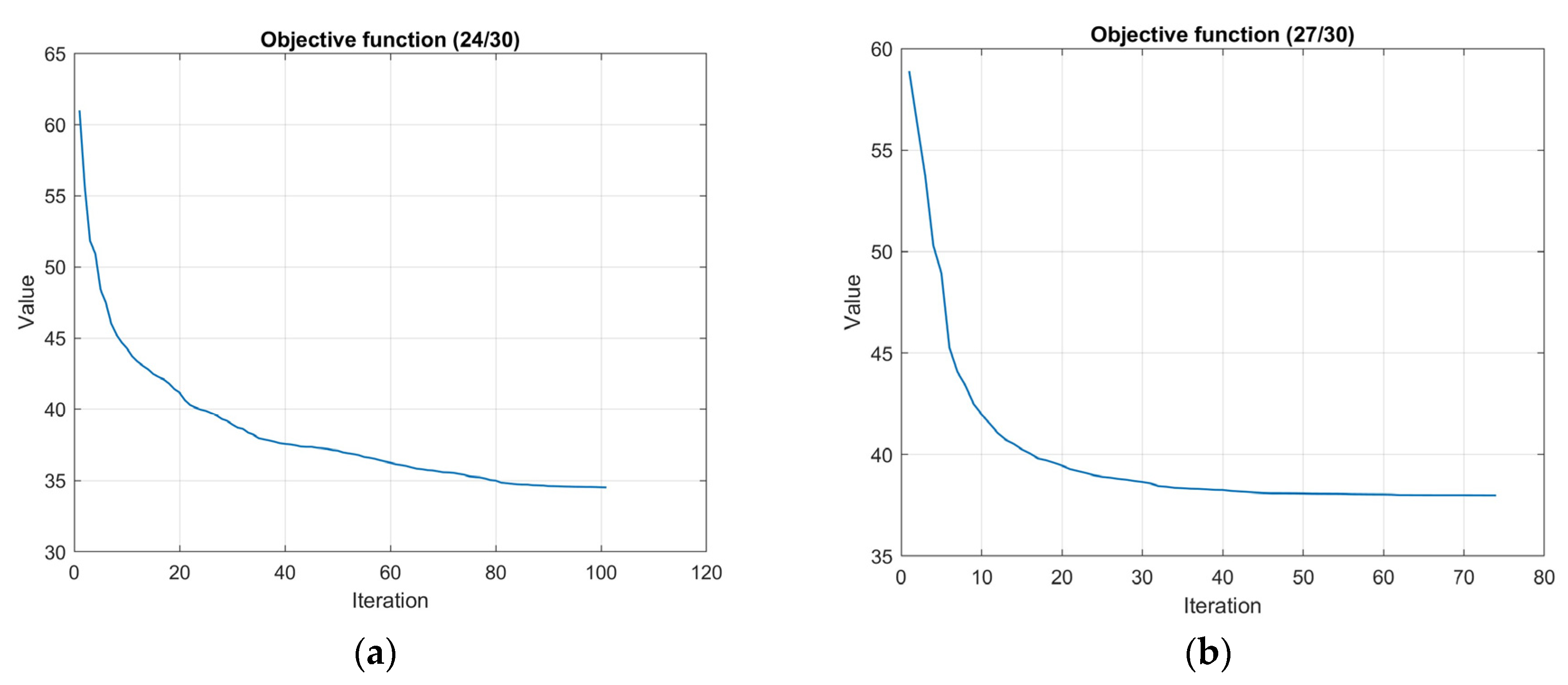
Figure 14.
Case study 3: Optimal node locations.
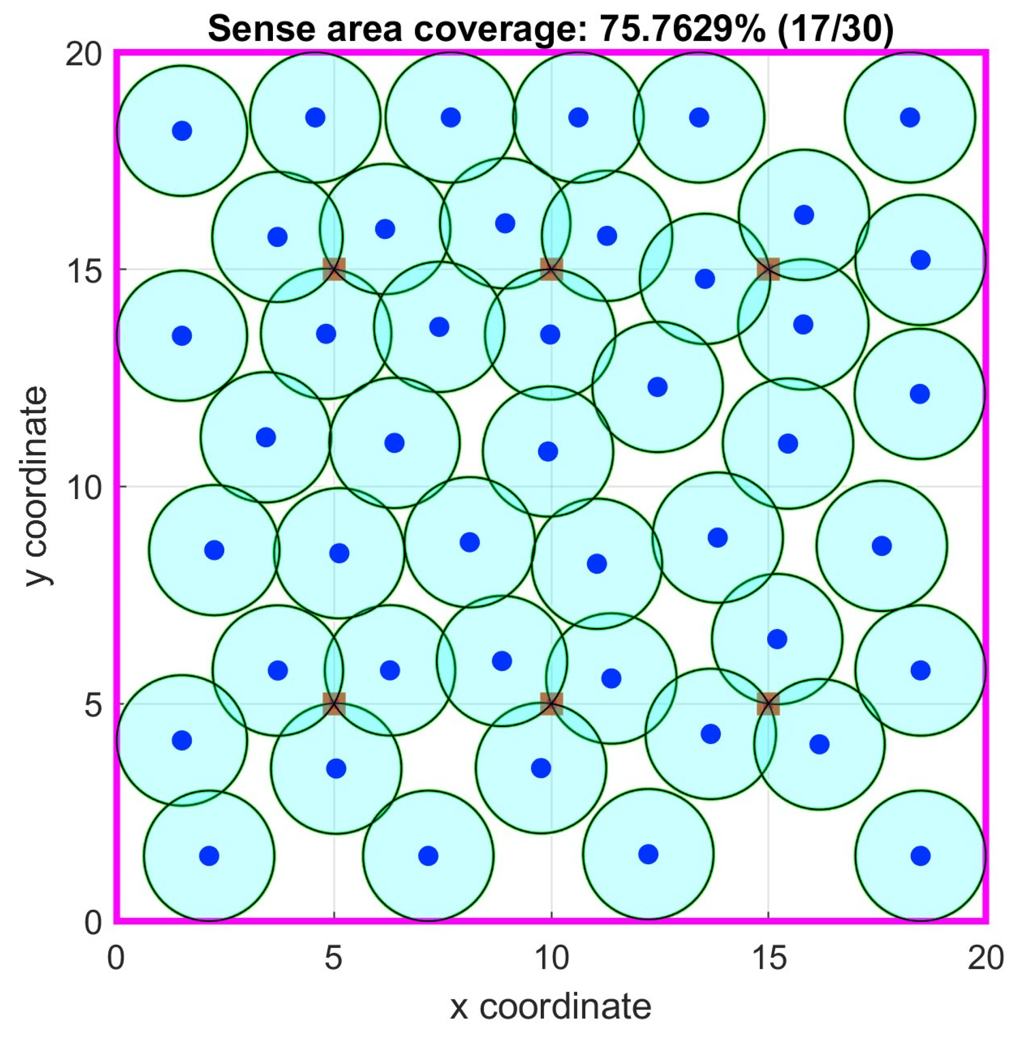
Figure 15.
Case study 3: Optimal node locations with 1-connectivity.
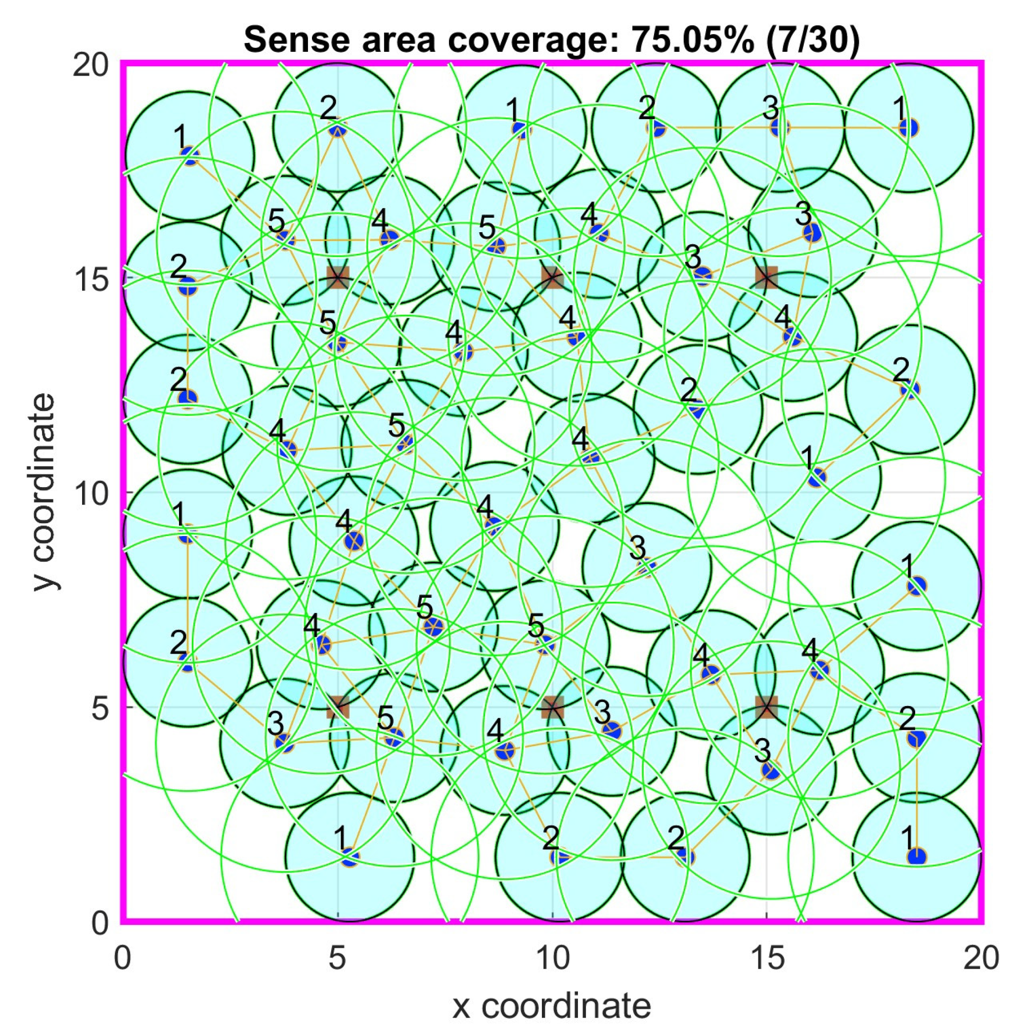
Figure 16.
Case study 3: Objective function iterations (a) No connectivity; (b) 1-connectivity.
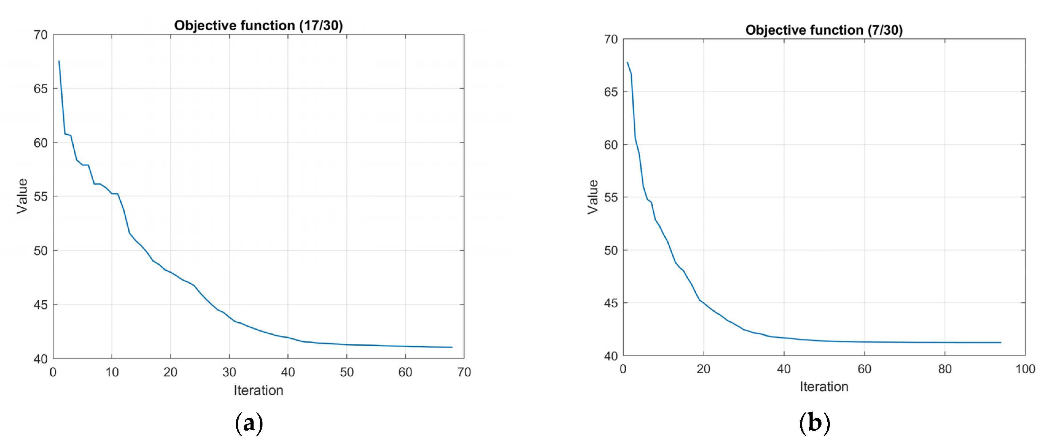
Figure 17.
Case study 4: Optimal node locations.
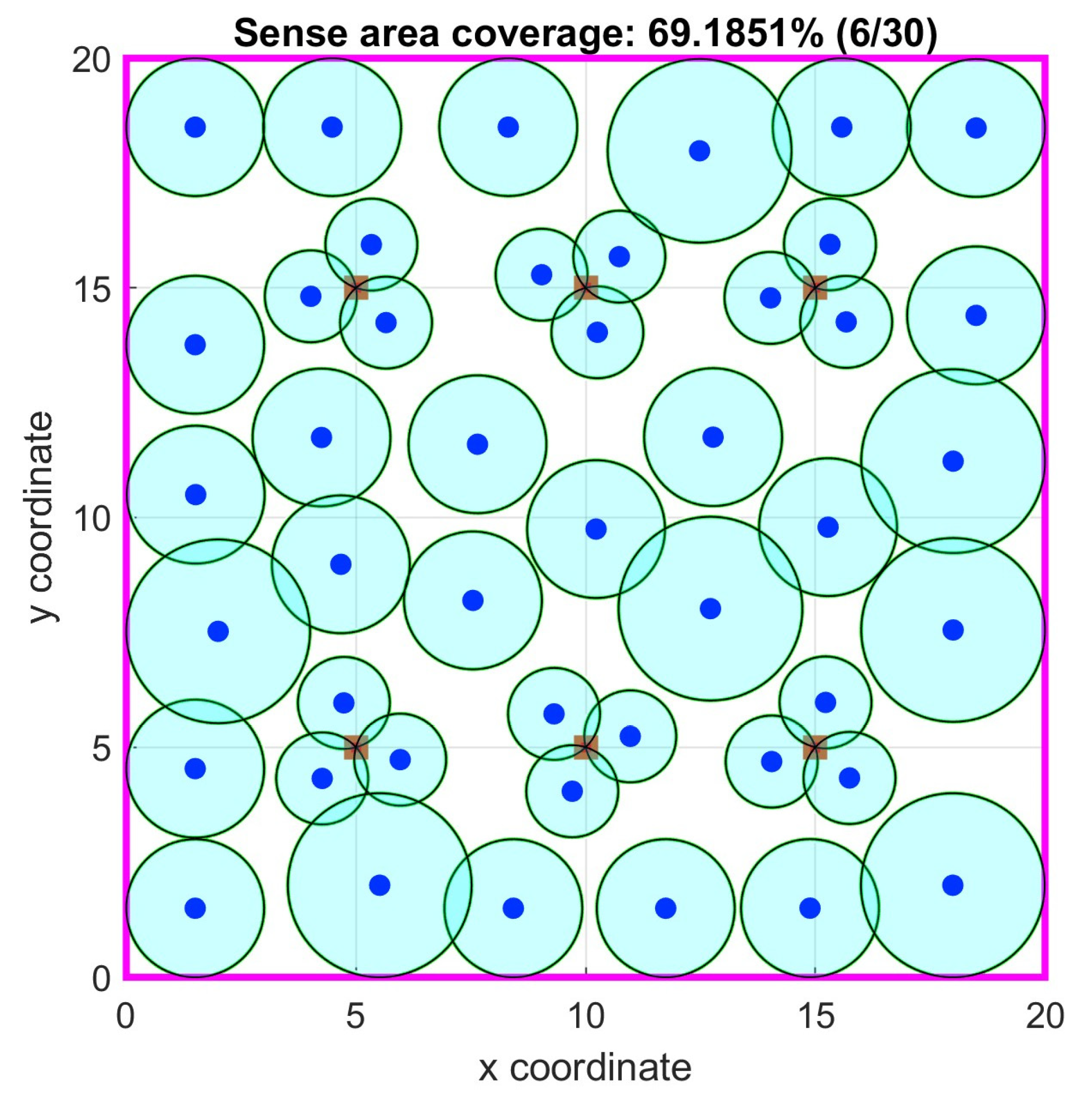
Figure 18.
Case study 4: Optimal node locations with 1-connectivity.
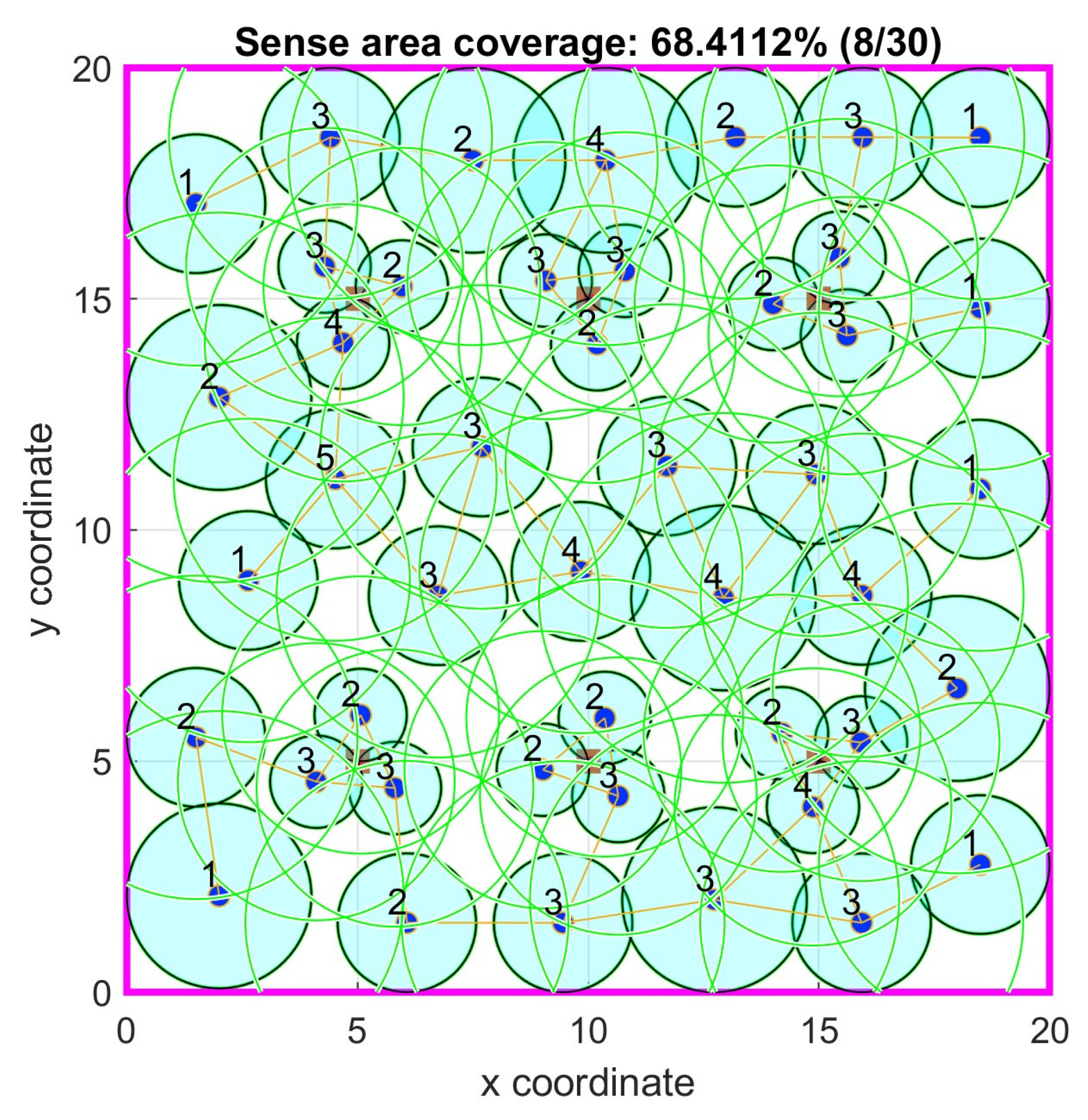
Figure 19.
Case study 4: Objective function iterations (a) No connectivity; (b) 1-connectivity.
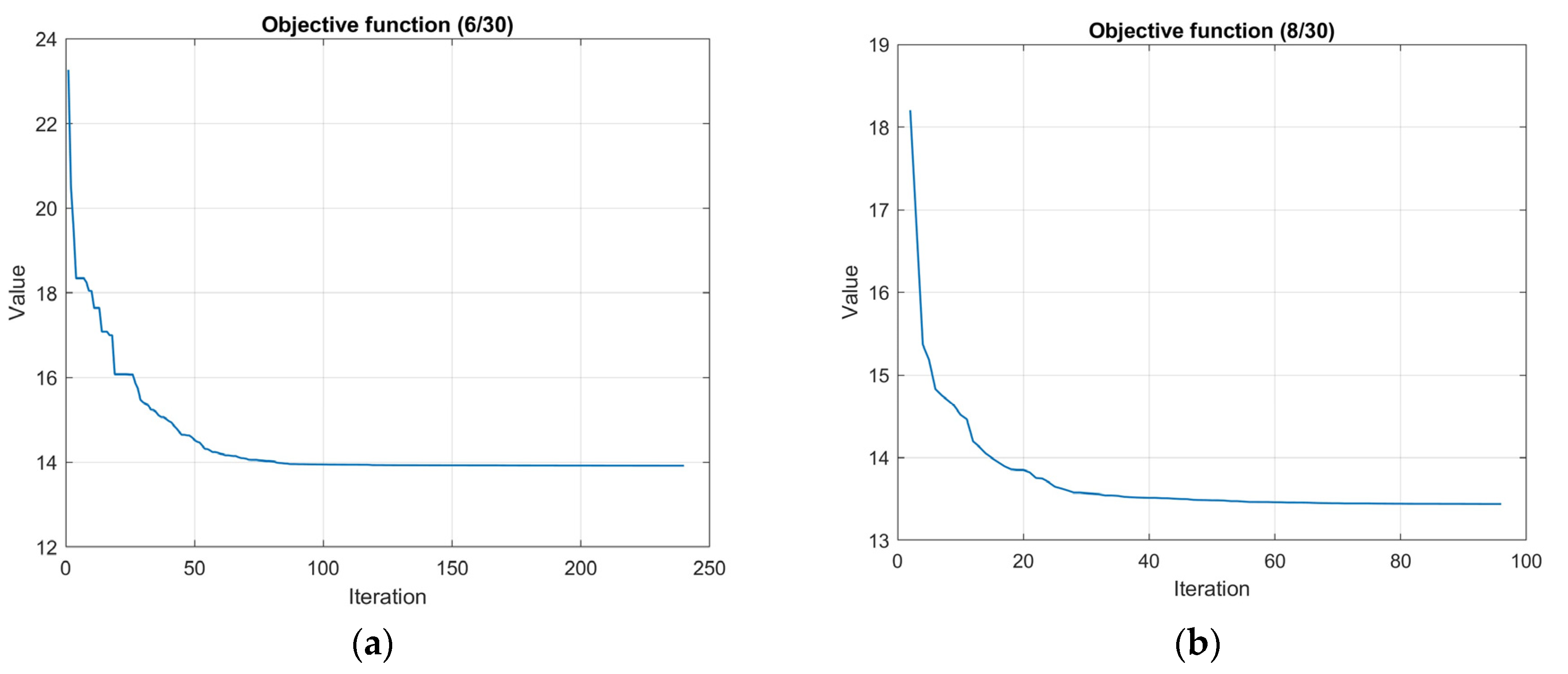
Figure 20.
Case study 5: Optimal node locations.
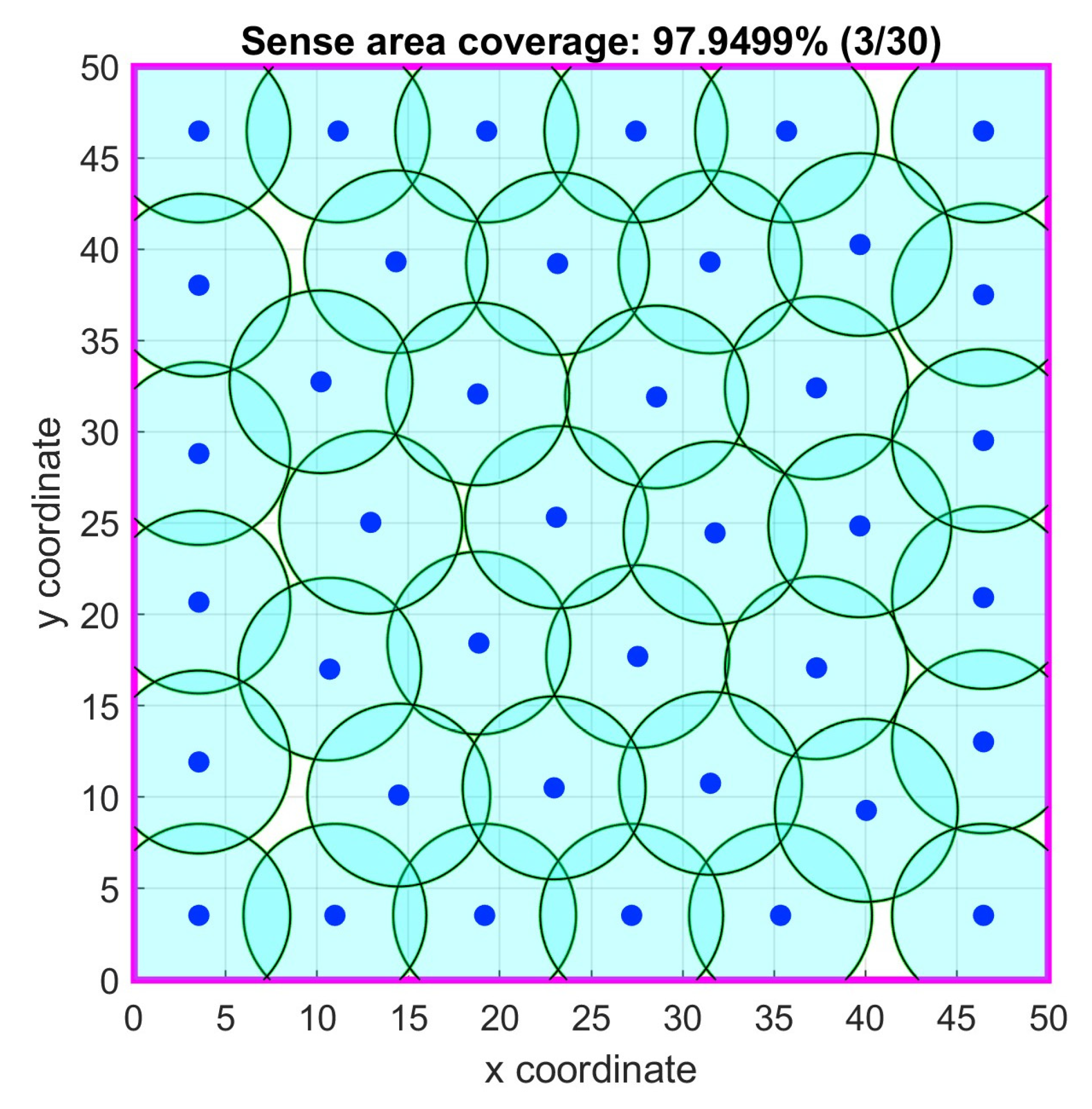
Figure 21.
Case study 5: Optimal node locations with 1-connectivity.

Figure 22.
Case study 5: Objective function iterations (a) No connectivity; (b) 1-connectivity.
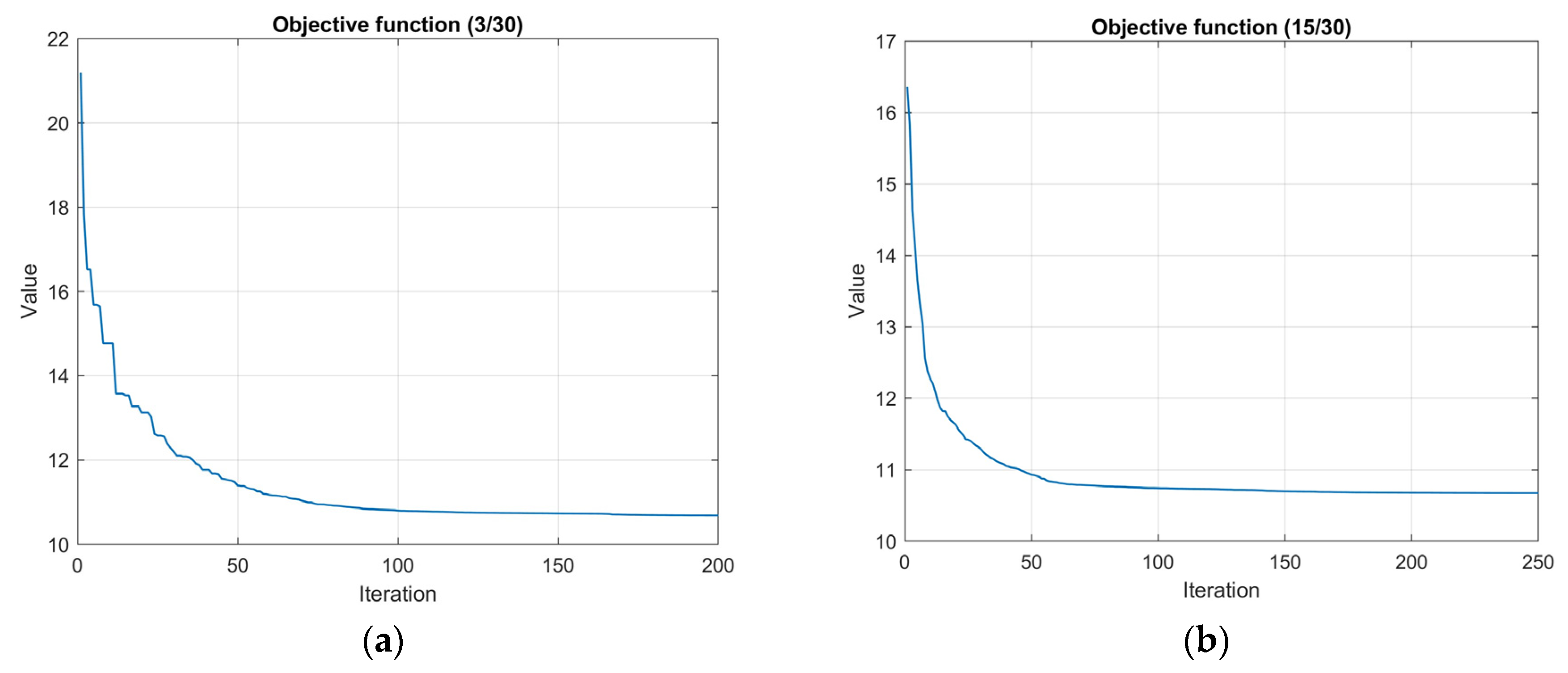
Figure 23.
Case study 6: Optimal node locations.
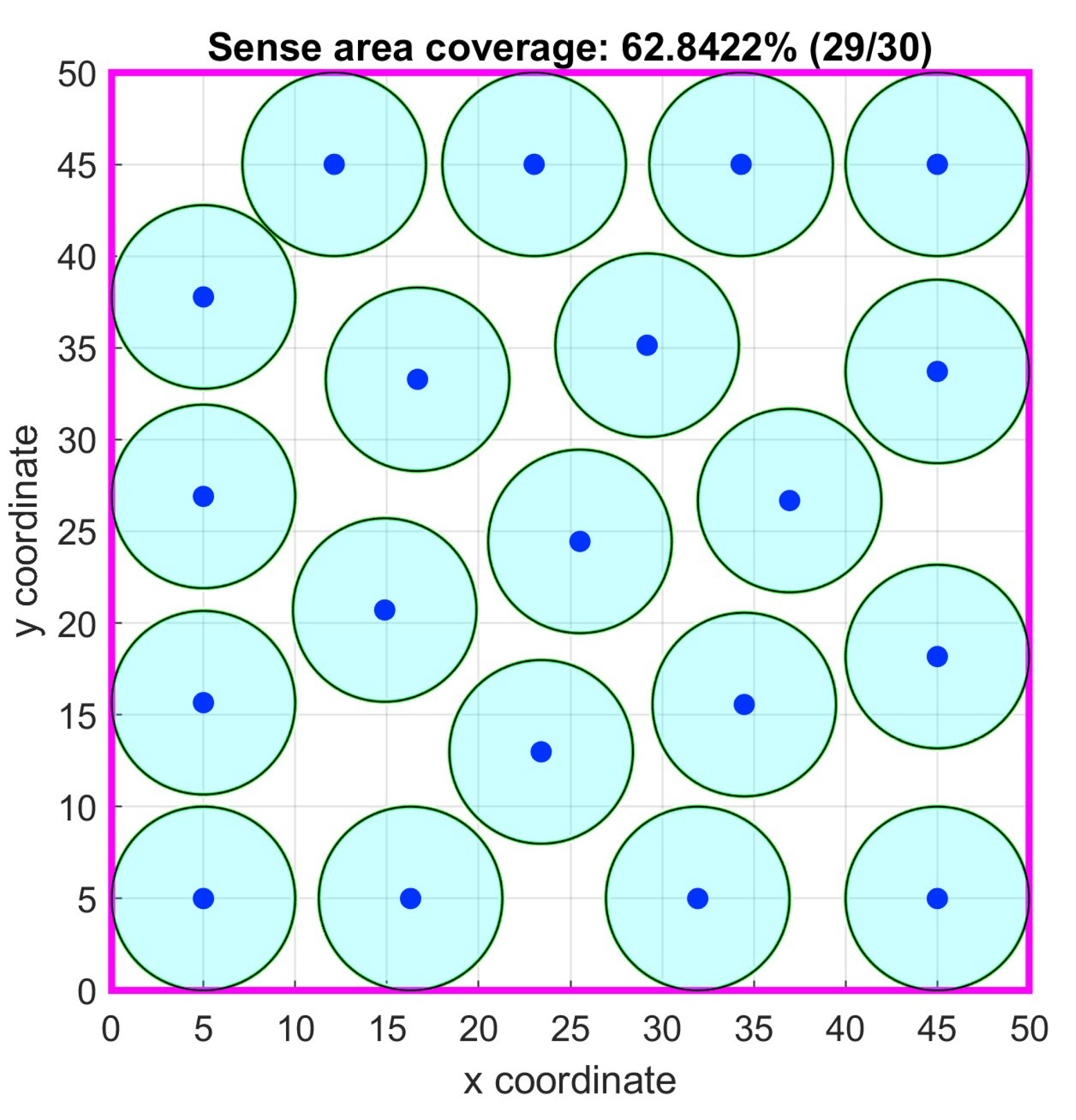
Figure 24.
Case study 6: Optimal node locations with 1-connectivity.
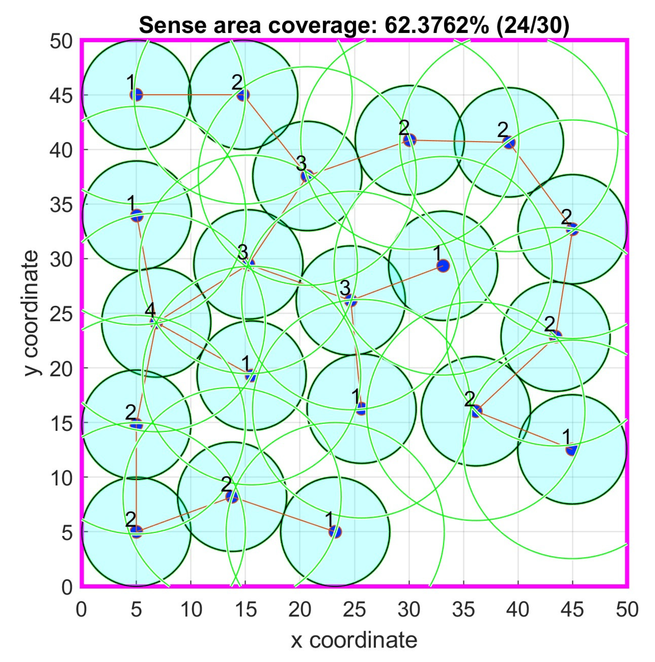
Figure 25.
Case study 6: Objective function iterations (a) No connectivity; (b) 1-connectivity.
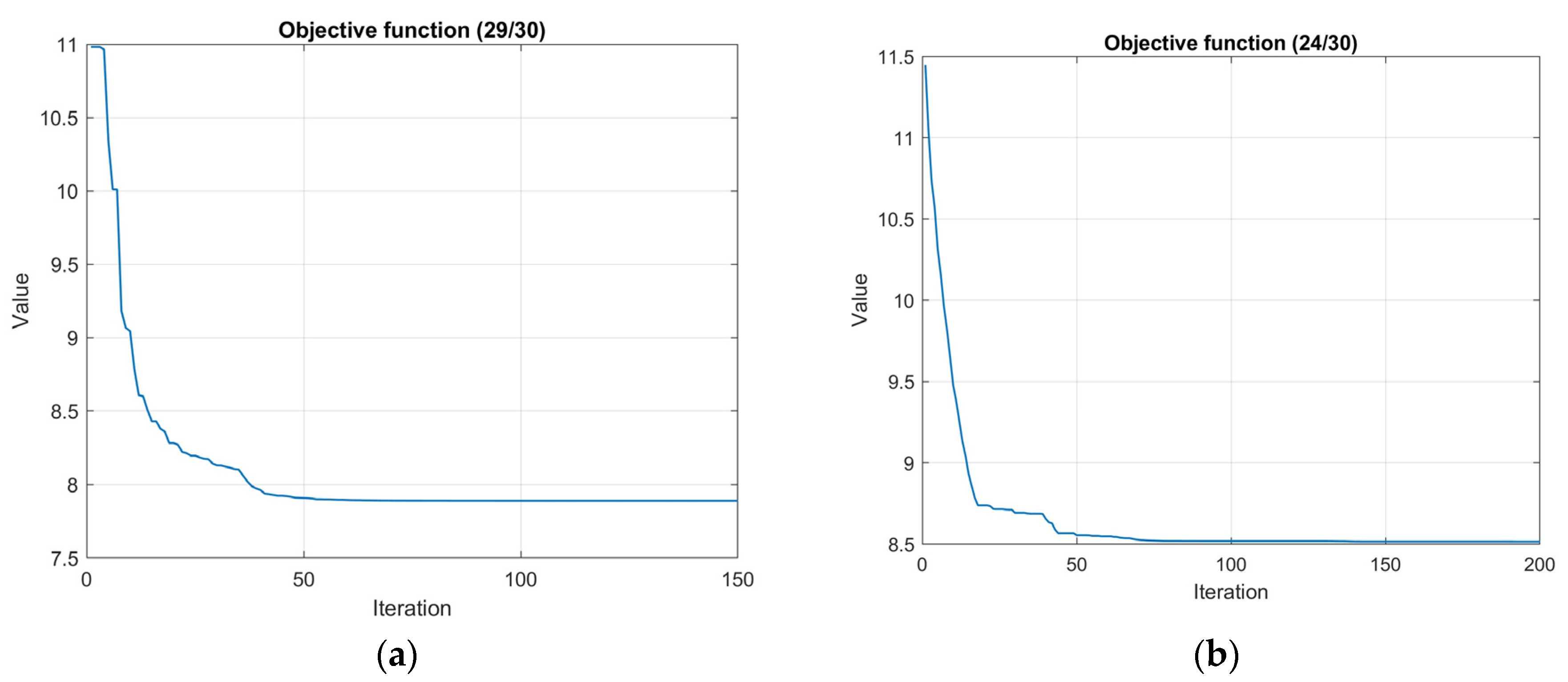
Figure 26.
Case study 7: Optimal node locations.
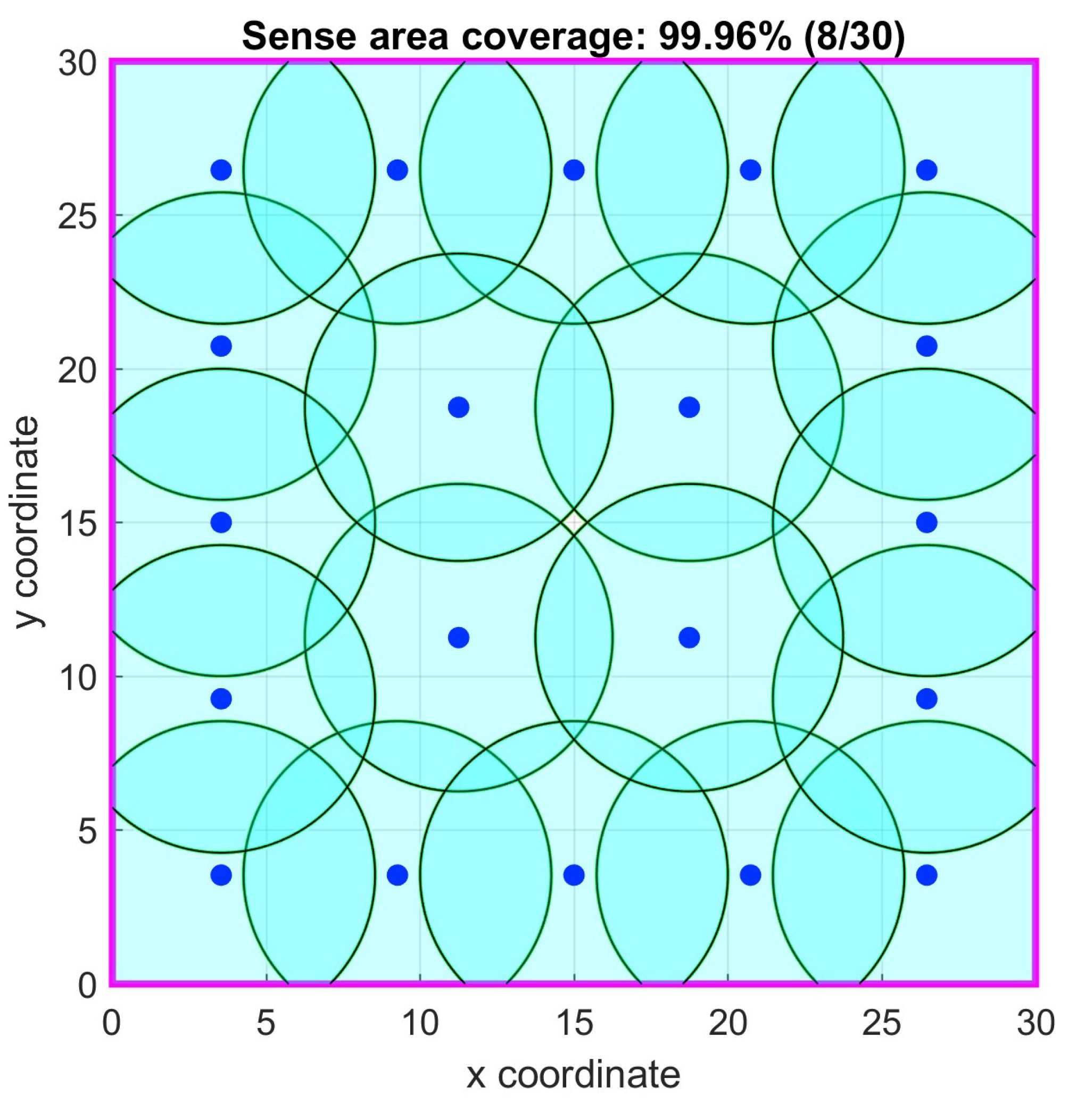
Figure 27.
Case study 7: Optimal node locations with 1-connectivity.
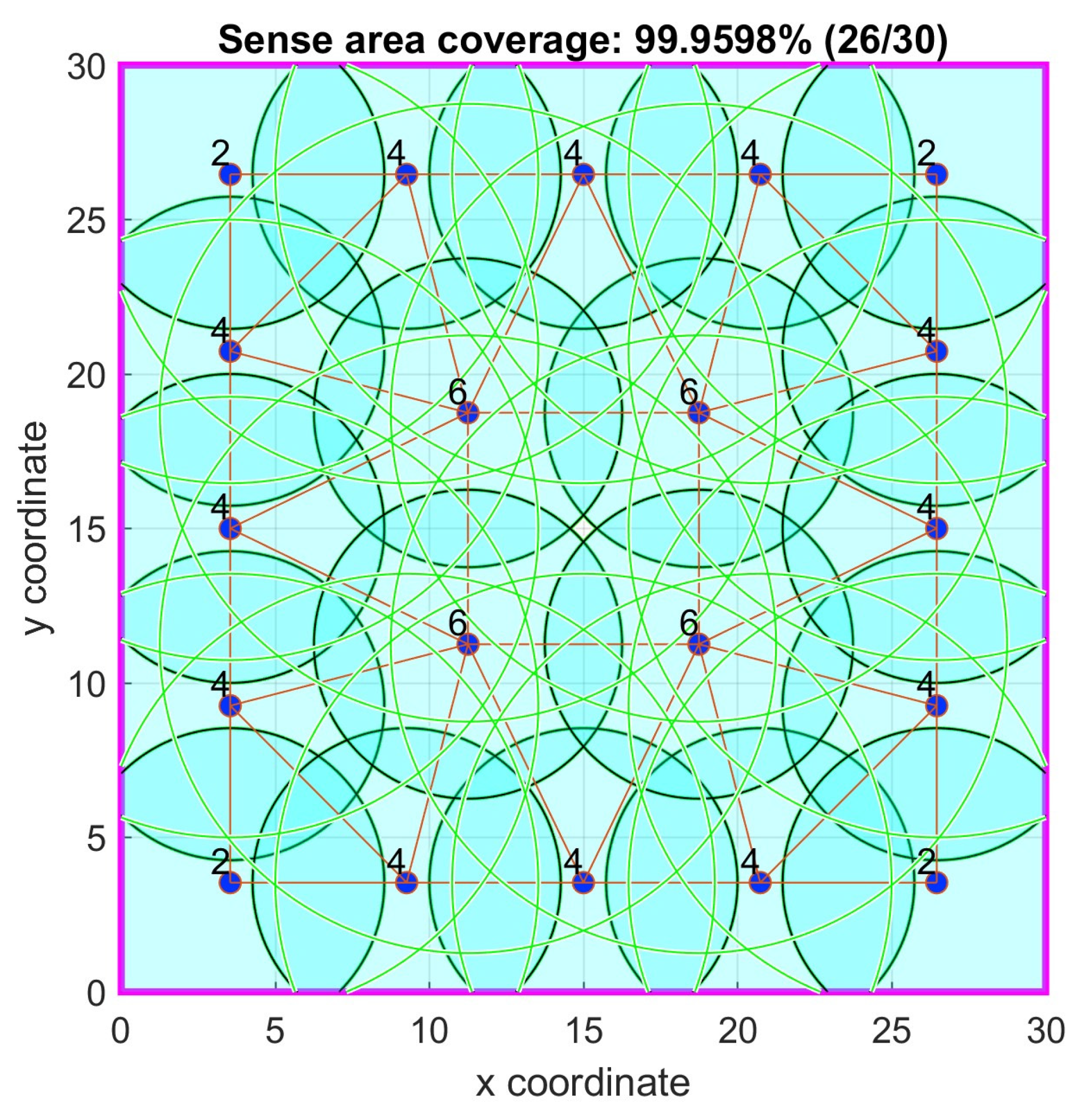
Figure 28.
Case study 7: Objective function iterations (a) No connectivity; (b) 1-connectivity.
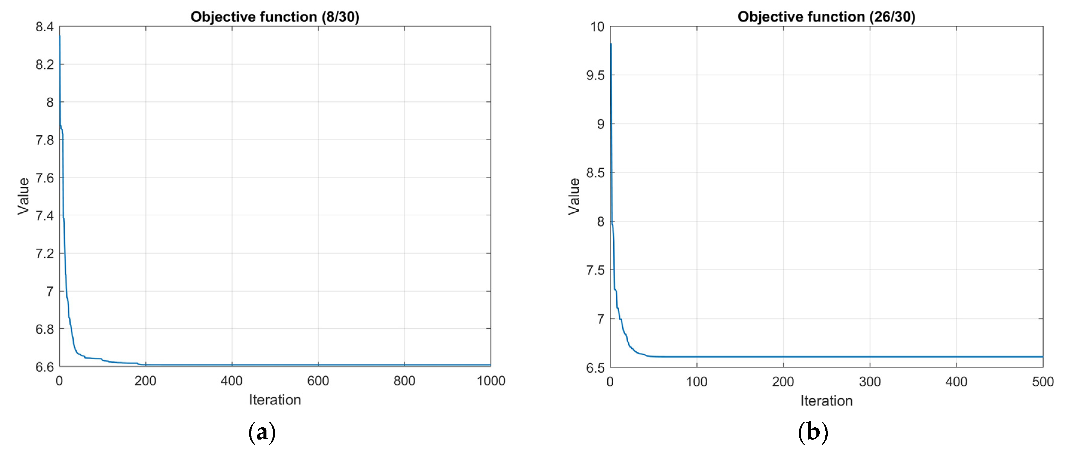

Table 1.
Case study 1: Simulation results.
| Parameter | GA[38] | PSO[38] | PSO No Conn | PSO 1-Conn |
|---|---|---|---|---|
| Mean Value | 61.17 | 60.92 | 61.79 | 61.49 |
| Standard Deviation | 0.28 | 0.46 | 0.12 | 0.15 |
| Best Fitness | 61.56 | 61.49 | 61.86 | 61.73 |
| p-Value | 0.00 | |||
| Ideal Coverage | 61.86 | |||
Table 2.
Case study 2: Simulation results.
| Parameter | GA[38] | PSO[38] | PSO No Conn | PSO 1-Conn |
|---|---|---|---|---|
| Mean Value | 59.37 | 58.83 | 59.44 | 57.77 |
| Standard Deviation | 0.18 | 0.38 | 0.27 | 0.62 |
| Best Fitness | 59.69 | 59.32 | 59.85 | 58.85 |
| p-Value | 0.00 | |||
| Ideal Coverage | 59.85 | |||
Table 3.
Case study 3: Simulation results.
| Parameter | GA[38] | PSO[38] | PSO No Conn | PSO 1-Conn |
|---|---|---|---|---|
| Mean Value | 73.07 | 72.13 | 74.21 | 72.69 |
| Standard Deviation | 0.66 | 0.85 | 0.98 | 1.45 |
| Best Fitness | 74.28 | 73.77 | 75.76 | 75.05 |
| p-Value | 0.00 | |||
| Ideal Coverage | 79.52 | |||
Table 4.
Case study 4: Simulation results.
| Parameter | GA[38] | PSO[38] | PSO No Conn | PSO 1-Conn |
|---|---|---|---|---|
| Mean Value | 67.39 | 69.89 | 67.69 | 65.72 |
| Standard Deviation | 0.45 | 1.15 | 0.97 | 1.64 |
| Best Fitness | 68.24 | 71.46 | 69.19 | 68.41 |
| p-Value | 0.066* | |||
| Ideal Coverage | 71.47 | |||
* p-Value comparing with the GA[38] algorithm.
Table 5.
Case study 5: Simulation results.
| Parameter | GA[38] | PSO[38] | PSO No Conn | PSO 1-Conn |
|---|---|---|---|---|
| Mean Value | 96.40 | 95.53 | 97.37 | 97.58 |
| Standard Deviation | 0.59 | 0.66 | 0.29 | 0.20 |
| Best Fitness | - | - | 97.95 | 98.02 |
| p-Value | 0.00 | |||
| Ideal Coverage | 100 | |||
Disclaimer/Publisher’s Note: The statements, opinions and data contained in all publications are solely those of the individual author(s) and contributor(s) and not of MDPI and/or the editor(s). MDPI and/or the editor(s) disclaim responsibility for any injury to people or property resulting from any ideas, methods, instructions or products referred to in the content. |
© 2024 by the authors. Licensee MDPI, Basel, Switzerland. This article is an open access article distributed under the terms and conditions of the Creative Commons Attribution (CC BY) license (http://creativecommons.org/licenses/by/4.0/).
Copyright: This open access article is published under a Creative Commons CC BY 4.0 license, which permit the free download, distribution, and reuse, provided that the author and preprint are cited in any reuse.


