Submitted:
26 April 2023
Posted:
27 April 2023
You are already at the latest version
Abstract
To address the problem that it is easy to form coverage blind areas when wireless sensor networks are randomly deployed, an improved coverage optimization algorithm based on improved Salpa swarm Intelligent algorithm (ATSSA) is proposed for wireless sensor networks. Firstly, the pop-ulation is initialized using tent chaotic sequence to enhance the optimization ability of the algo-rithm. Secondly, the T-distribution mutation is added to the update formula of the leaders for improving the ability to jump out of the local optimal value. Finally, an adaptive formula for updating the position of the follower is proposed, which not only guarantees the local searching ability of the algorithm in the late iteration period, but also improves the global searching ability of the algorithm in the early iteration period. The experimental results show that ATSSA algorithm can improve the coverage of the wireless sensor networks and reduce deployment costs com-pared with other algorithms, when it is used in the wireless sensor networks.
Keywords:
wireless sensor network (WSN)
; Salp Swarm Algorithm (SSA)
; T-distribution
; tent chaotic se-quence
1. Introduction
Wireless sensor network (WSN) is self-organizing network which is composed of a large number of low-power sensor nodes by wireless communication [1,2]. These sensor nodes have the ability of communication, calculation and perception which are easy to be deployed and have low cost and power consumption [3]. In recent years, WSN has been widely used in military, industrial, environmental detection, disaster relief, and other fields [4,5,6,7]. It provides great convenience for human life. By deploying it at scale within a region, information within a region can be collected and processed. The aim of the present study is to deploy a minimum number of sensor nodes to monitor a specific target area of interest. When wireless sensor network nodes need to be deployed to complex and harsh environments, random throwing deployment are often used to deploy wireless sensor network nodes. However, the random throwing deployment is easy to form coverage blind areas, resulting in low node utilization, waste of resources, and degradation of detection quality [8]. Therefore, it is necessary to optimize the coverage mode of wireless sensor network, so that the sensor nodes are evenly distributed and blind areas of the network coverage are reduced, in order to improve the coverage efficiency of wireless sensor network and reduce network construction costs.
In recent years, many new intelligent optimization algorithms have been proposed. Many scholars have improved them and applied them to the deployment optimization problems of WSN, and have obtained good results [9,10,11,12,13]. Literature [14] proposes an improved COOT Bird Algorithm to optimize the deployment of WSN nodes, which solves the problem that the original algorithm is easy to fall into local optimization and improves the coverage of the algorithm. Literature [15] used the ALO algorithm to address the problems of uneven node distribution and incomplete coverage in node deployment. Literature [16] proposed a new 3D improved virtual force coverage (3D-IVFC) algorithm for 3D coverage of nodes in WSN. It improves the coverage of WSN and shortens the deployment time of sensor nodes. There are still problems such as premature convergence, low local search ability, and inability to balance global search and local search ability. So, the node coverage can still be further improved.
Salp Swarm Algorithm (SSA) is a new type of swarm intelligence optimization algorithm proposed by Australian scholar Mirjalili in 2017 [17]. It has the advantages of less parameters and better balance between the local search and global search capabilities. This algorithm is widely used in path planning, image processing, photovoltaic systems and other fields. However, the original SSA algorithm also has the disadvantages of relying on the initial population, slow convergence speed, and easy to fall into local optimization. In this regard, scholars at home and abroad have proposed many improved SSA algorithm. Literature [18] introduces a novel hybrid algorithm inspired by the perturbation weight mechanism. The algorithm overcomes the the problems of poor real-time performance and low precision of the basic salp swarm algorithm. Literature [19] integrates random pair multiple leadership and simulated annealing mechanism in the SSA, so that the SSA can be applied to complex multimodal problems. The literature [20] adds an inertia weight to the leader update formula of the SSA. It improves the classification accuracy and feature reduction ability of the algorithm compared with other algorithms.
Because the original SSA algorithm has slow convergence speed and easily falls into local optimum. In order to better apply it to the deployment optimization problem of WSN, this paper proposes an adaptive salp swarm algorithm (ATSSA) based on the tent chaotic sequence and T-distribution mutation. The ATSSA is applied to node deployment optimization of WSN to improve the coverage rate of WSN sensor nodes.
2. WSN Node Coverage Model
This article assumes that the target area A monitored by the wireless sensor network is a rectangle with an area of . It is a two-dimensional area. The set of nodes can be denoted as ,, and the coordinates of each node can be denoted as , where .
For a two-dimensional wireless sensor network, its network model is as follows:
- Each sensor node has the same parameters, structure, and communication capabilities.
- Each sensor node has normal communication functions, sufficient energy and can move freely.
- Each sensor node can obtain data information and update the location information in time.
- The sensing radius of each sensor node is and the communication radius is , both in units of meters, and .
The sensing range of a sensor node is represented by a circular area with the node at its center and the radius equal to the sensing range. In this two-dimensional wireless sensor network (WSN) monitoring area, if there are n target monitoring points, the set of target monitoring points can be denoted as , and the location coordinate of each target point is , where . If the distance between a target node and any sensor node is less than or equal to the sensing radius , it means that is covered. The Euclidean distance between sensor node and target monitoring point is defined as:
The node-sensing model in this paper is a Boolean sensing model. When the sensing radius is greater than or equal to , the probability that the target is monitored is 1; otherwise, the probability that the target is monitored is 0. If the probability that the target point to be monitored is covered by the sensor node be p, then
In this 2D wireless sensor network (WSN) monitoring area, sensor nodes can collaborate with one another. Each monitoring point can be covered by multiple sensors simultaneously, so the probability that any monitoring target point is jointly sensed is:
The coverage rate can be defined as the ratio of the coverage area of all sensor nodes within the monitoring area to the total area of the monitoring area. Therefore, in the case of a 2D WSN monitoring area, the coverage rate can be calculated as follows:
The node coverage optimization problem for WSN can be described by an integer linear programming model, the model is as follows:
3. Salp Swarm Algorithm
The inspiration of the intelligent optimization algorithm of salps group comes from the aggregation behavior of salps group in the ocean, namely salps chain. Salp squirts feed on the phytoplankton in the water and move through the water by breathing in and spewing out seawater. The SSA algorithm mimics the foraging behavior of the organism. The population of SSA algorithm is divided into two groups. These two groups are leader and followers. The leaders take the position at the front of the chain, while the remainders of salps are known as followers. dim refers to the number of variables or dimensions in a given problem, and x represents the position of a salp. F denotes the food source, which is the target of the swarm in the search space.The leader updates his position according to the following equation:
Where, is the food source in the jth dimension, and is the upper and lower bounds of the search space, and is a random number between [0,1], determines the length of the individual's next position movement, and determines whether the movement direction is positive or negative. is the main parameter that balances the ability to search and exploit in evolution, and its formula is as follows:
where T is the current iteration number, and is the maximum number of iterations. The follower position is updated according to Newton's law of motion, which is formulated as follows.
where, is the position of the th salp individual in the j-dimensional space, , is time, v0 is initial velocity, and acceleration is as follows:
Since is the difference between the two iteration times, unit time is desirable, and the initial velocity , Equation (7) can be expressed as follows:
4. Improved Salp Swarm Algorithm
4.1. Population initialization and the chaotic tent map
Chaotic variables have the characteristics of randomness, ergodicity and regularity, which have been used by many scholars to optimize search problems [21]. Chaotic variables can not only effectively maintain the diversity of populations, but also help the algorithm to jump out of the local optimal and improve the global search ability. The initial population is evenly distributed in the search space, which is of great help to the algorithm optimization. When the SSA population is initialized, most of them are randomly generated. So, using chaotic sequence to initialize the SSA population can improve the convergence speed of SSA algorithm.
The basic idea of chaotic sequences is to generate sequences between [0,1] by mapping, and then transform them into the search space of individuals. Among various chaotic models, tent map can generate better uniform sequences. Therefore, this paper uses tent chaotic sequence to initialize the population of SSA algorithm, and its formula is as follows:
As shown in Figure 1 and Figure 2, is a chaos parameter that controls tent chaotic sequence. According to the value of the parameter µ, the bifurcation diagram and Lyapunov exponential curve of the chaotic tent map are drawn. In Figure 1, it can be seen that when the chaotic tent map produces an approximately uniformly distributed chaotic sequence. In Figure 2, when ,the Lyapunov exponent curve is greater than 0. So, in this article, . represents the number of iterations, represents the population size.
In this paper, the chaotic sequence is set to N d-dimensional arrays, where d is the dimension of the salp swarm population. After iterating for i times, yi j is obtained. It is inversely mapped to the corresponding individual search space, and the variable is obtained, and the formula is as follows:
4.2. Positions updating
4.2.1. Positions updating of the leaders and adaptive t-distribution
The Gaussian Distribution (GD) and Cauchy Distribution (CD) are two boundary special cases of the T-distribution [22,23]. In terms of performance, the Gaussian distribution has strong local development ability, Cauchy distribution has strong global search ability, and the T-distribution has the advantages of both Gaussian distribution and Cauchy distribution [24]. The formula of probability density function of T-distribution with the adaptive parameter is as follows:
The T-distribution degree-of-freedom parameter is set to the number of iterations. When T=1, the T-distribution is the standard Cauchy distribution. When the iteration starts, the T-distribution and the Cauchy distribution are more similar, and the global search ability is stronger. With the increase of T, the T-distribution gradually changes from Cauchy distribution to transforms into a Gaussian distribution, and the local search ability is stronger at this time, and the convergence speed of the algorithm is accelerated.
Figure 3 shows that the mutation probability at both ends of the t-distribution curve with a degree of freedom parameter of 5 is smaller than that of the curve with a degree of freedom parameter of 3. The mutation probability near the origin with the degree-of-freedom parameter 5 is greater than the mutation probability near the origin with the degree-of-freedom parameter 3. From the above analysis, it can be seen that with the increase of the degree-of-freedom parameters, the probability of large disturbances in the early stage of iteration is greater than that in the late stage of iteration, so it has better global exploration ability. Compared with the early iteration, the probability of small disturbance is greater in later stage. In this stage, the curve of T-distribution has better local exploration ability and accelerates the convergence speed of the algorithm.
The mutation strategy is a common improvement strategy used to jump out of the local optimal solution of the meta-heuristic algorithm. In this article, adaptive T-distribution mutation is used to enhance the ability of the SSA to jump out of local optimal solutions, and accelerate the convergence speed of SSA. The update formula of the leader of the SSA algorithm is improved with the T-distribution., and the parameter is replaced by , the new leader position update formula after replacement is as follows:
where is the step control parameter, which controls the displacement length within 1, and this paper .
4.2.2. Positions updating of the followers
The SSA performs local search by updating the follower location. In the SSA, the number of individual leader and follower are always split equally. In the early stage of algorithm iteration, the global search capability of the algorithm is increased by adjusting the update formula of followers. With the continuous iteration of the algorithm, the local search ability of the algorithm is gradually restored. Therefore, this paper adopts an adaptive strategy to update the follower's position, which improves the follower's global search ability in the early stage and ensures its local search ability in the later stage. The improved follower position update formula is as follows:
where is an one-dimensional vector whose length is the population dimension . Vector update formula is as follows:
is an adaptive parameter that controls whether the follower is affected by the vector P, and its update formula is as follows:
where γ is a random number between [0,1], η is the control parameter, which controls whether the follower performs a global search or a local search, the value in this article is 0.3. When ω is 1, the followers’ positions are updated through the vector, and when ω is 0, the follower performs the local search with equation (11).
4.3. Implementation Steps of ATSSA
Step 1: Set the parameters of population size n, maximum number of iterations , upper bounds ub and lower bounds lb of the detection region, etc.
Step 2: Randomly initialize the positions of Salp Swarm and Enhance the diversity of the population by using the tent chaotic sequence in Equation (11).
Step 3: Take coverage Cov as the objective function, calculate the fitness value of each individual, and find the best individual as the initial food source.
Step 4: Update the position of leaders and followers according to Equation (15) and (16).
Step 5: Calculate the fitness value of each individual of the population, and update the food source and food source location.
Step 6: Determine whether the end condition is reached; if yes, proceed to the next step; otherwise, return to Step 4.
Step 7: The program ends and outputs the optimal fitness value and the best position.
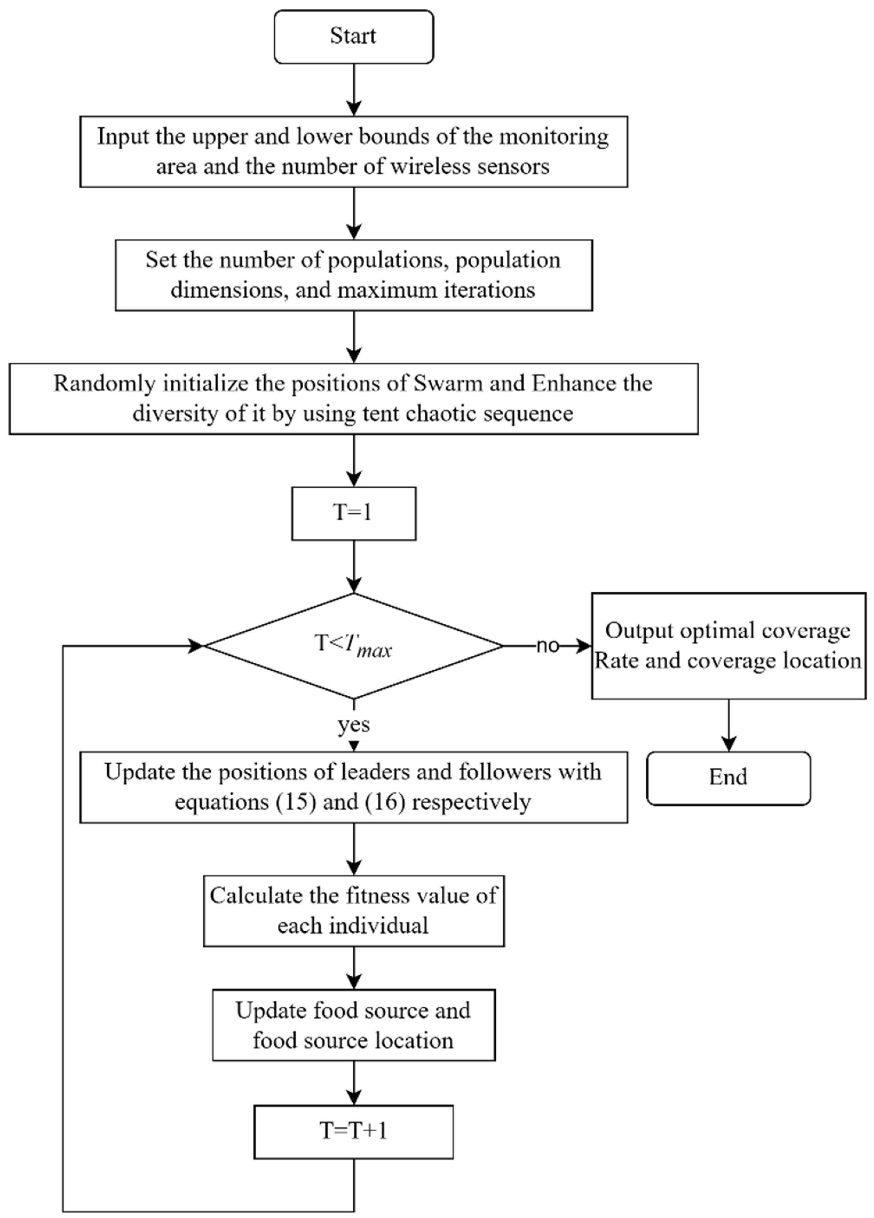
5. Coverage Optimization Strategy
The coverage optimization strategy of WSN based on ATSSA abstracts the coverage optimization problem of WSN into a high-dimensional vector maximum optimization problem of ATSSA with as the objective function. The problem of wireless sensor location optimization in WSN coverage optimization is abstracted into the problem of food source search by the salp swarm. The final food source is the optimal coverage, and the food source is the location of wireless sensor. In the SSA, each individual of the salp swarm is a WSN coverage distribution. If the number of wireless sensors is n, the population dimension of the salp swarm is 2n, where the 2i and 2i-1 represent the ordinate and abscissa of the ith node respectively. The specific strategies are as follows:
Step 1: Input the upper and lower bounds of the monitoring area and the number of wireless sensors.
Step 2: Set the number of populations, population dimensions, and maximum iterations.
Step 3: Randomly initialize the positions of Swarm and Enhance the diversity of it by using the tent chaotic sequence.
Step 4: Update the position of leaders and followers with Equation (15) and (16).
Step 5: Calculate the fitness value of each individual of the population, and update the food source and food source location.
Step 6: Determine whether the end condition is reached; if yes, proceed to the next step; otherwise, return to Step 4.
Step 7: The program ends and outputs the optimal coverage Rate and coverage location.
Figure 4.
Flowchart of the ATSSA coverage optimization algorithm.
6. Simulation Experiments and Analysis
In order to verify the effectiveness of the improved strategy of ATSSA algorithm and the performance of the algorithm, this paper sets up two experiments. Experiment 1 applies ATSSA algorithm, SSA algorithm [17], HHO algorithm [25] and WOA algorithm [26] to the coverage optimization of wireless sensor networks, the same parameters are set, and the four algorithms are respectively applied to the coverage optimization of wireless sensor networks to test the performance of ATSSA algorithm. Experiment 2 compares the minimum number of nodes required by each algorithm to achieve a specific coverage rate through experiments, so as to verify whether the coverage optimization of ATSSA algorithm can effectively save the deployment cost of wireless sensor networks.
The experiment is simulated on Windows 10 operating system and Matlab 2019b. The parameters used in the four algorithms are shown in the following table (Table 1):
6.1. Experiment 1
In this experiment, two different target field were set up. It’ s aim is to compare the performance of the ATSSA with the performance of other algorithms.
6.1.1. Target Field 1
The monitoring area is set as 50m×50m, the sensing radius is set as 5m, the communication radius is set as 10m, the number of wireless sensor nodes is set as 40, and the maximum number of iterations is set as 500.

Table 2.
Experimental parameter settings for the node deployment area.
| Parameters | Values |
| Area of deployment | |
| Sensing radius | |
| Communication radius | |
| Number of sensor nodes | |
| Number of iterations |
In order to obtain universal results, ten experiments were conducted for each algorithm, and the average was taken as the result.
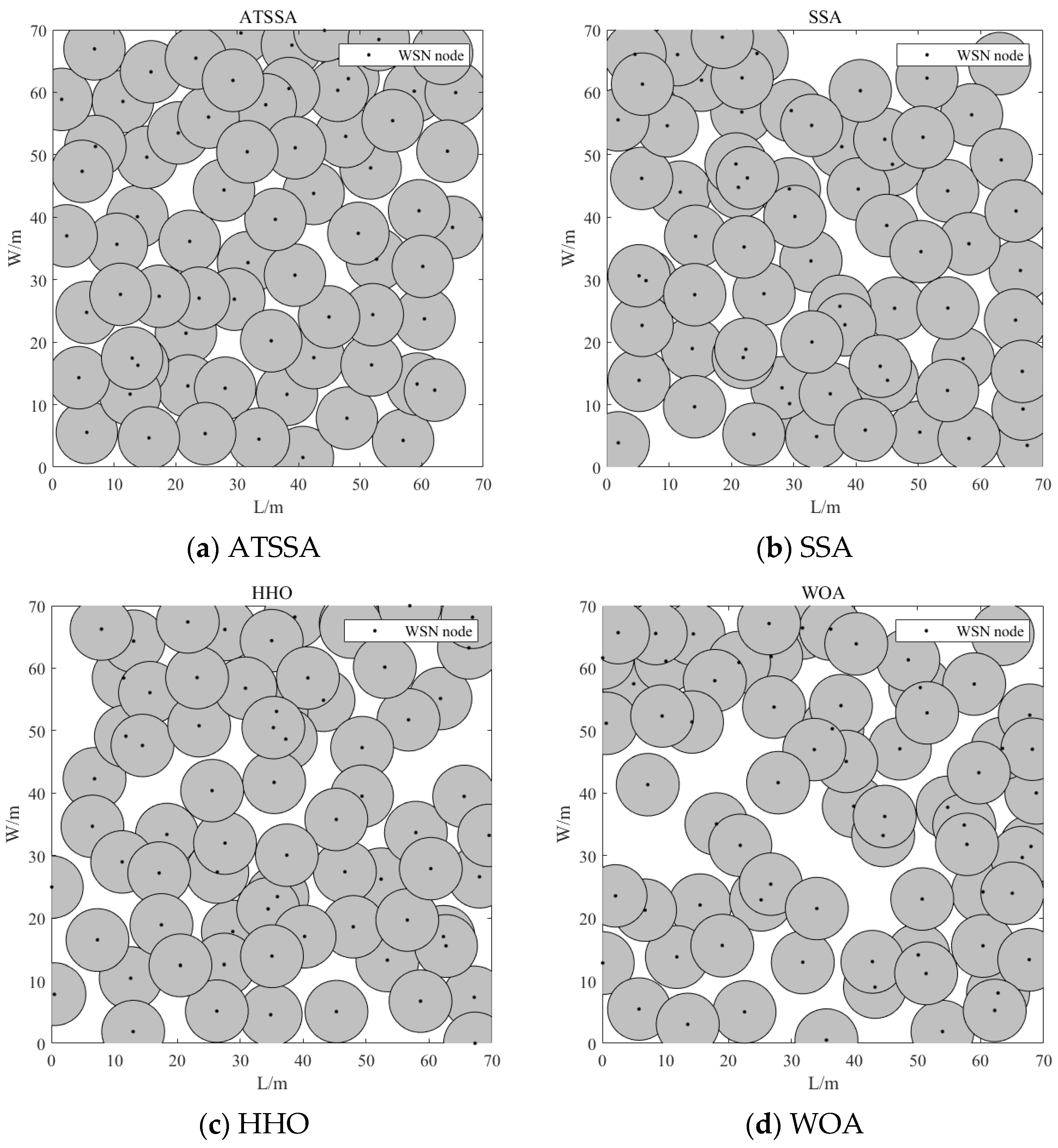
Figure 5 shows the deployment of wireless sensor network nodes obtained by using ATSSA algorithm(a), SSA algorithm (b), HHO algorithm (c) and WOA algorithm (d) respectively. As can be seen from the figure, compared with the other three algorithms, the deployment of sensor nodes after coverage optimization using ATSSA algorithm in this paper is more uniform. Figure 6 and Table 3 shows the optimization curve of coverage optimization using ATSSA algorithm, SSA algorithm, HHO algorithm and WOA algorithm respectively. It can be seen from the figure that WOA algorithm has fast convergence speed, but it is easy to converge prematurely, while HHO algorithm has strong global search ability, but it is difficult to converge. Compared with HHO algorithm and WOA algorithm, ATSSA algorithm and SSA algorithm have certain advantages in performance to improve the coverage efficiency of wireless sensor network. In the figure, when the algorithm starts, the coverage rate of ATSSA algorithm and SSA algorithm is similar. With the increase of iteration times, under the influence of the mutation mechanism of ATSSA algorithm, the convergence speed of ATSSA algorithm is obviously better than that of SSA algorithm. When the number of iterations reaches about 300, ATSSA algorithm and SSA algorithm tend to converge. The performance of ATSSA algorithm in coverage optimization of WSN is improved by about 3% compared with the original SSA algorithm.
6.1.2. Target Field 2
Set the monitoring area to 70m×70m, the sensing radius to 5m, the communication radius to 10m, the number of wireless sensor nodes to 40, and the maximum number of iterations to 1000.
Table 4.
Experimental parameter settings for the node deployment area.
| Parameters | Values |
| Area of deployment | |
| Sensing radius | |
| Communication radius | |
| Number of sensor nodes | |
| Number of iterations |
Figure 7.
Deployment of each algorithm node.
In order to obtain universal results, ten experiments were conducted for each algorithm, and the average was taken as the result.
Compared with scenario 1, this scenario expands the area area, the number of sensor nodes is increased, and the maximum number of iterations of the algorithm is set to 1000. As shown in the Figure 8 and Table 5, in a larger area, the ATSSA algorithm still has significant advantages over other algorithms. In the ten experiments, the highest coverage of ATSSA algorithm was about 89% and the lowest coverage rate was about 86%, while the coverage rate of SSA was about 86% and the lowest coverage rate was about 82%, indicating that ATSSA algorithm not only performed better than SSA, but also its stability was better than SSA algorithm.
6.2. Experiment 2
Set the monitoring area to , the sensing radius to 5m, the communication radius to 10m, and the maximum number of iterations to 500.
Table 6.
Experimental parameter settings for the node deployment area.
| Parameters | Values |
| Area of deployment | |
| Sensing radius | |
| Communication radius | |
| Number of iterations |
In order to obtain universal results, ten experiments were conducted for each algorithm, and the average was taken as the result.
Figure 9 and Table 7 show the number of nodes required for different algorithms to optimize under specific coverage. When the coverage rate reaches 80%, the number of nodes required by ATSSA algorithm, SSA algorithm, HHO algorithm and WOA algorithm is 27, 28, 30 and 33 respectively. The difference between the algorithms is small, and ATSSA algorithm has small advantages. With the increase of coverage rate, ATSSA algorithm can save more nodes than other algorithms. When the coverage rate reaches 95%, ATSSA algorithm saves 6, 9 and 18 sensor nodes respectively compared with other algorithms. This study shows that the optimized deployment of wireless sensor network nodes by ATSSA algorithm can achieve better coverage and save more sensor nodes than other algorithms.
7. Conclusions
Aiming at the problems of uneven node distribution and low coverage of the target monitoring area when randomly deploying sensor nodes in WSNs, an improved Salp Swarm Algorithm which named ATSSA for node coverage aptimization in WSNs is proposed in this paper. ATSSA uses the tent chaotic sequence to initialize the population based on the original Salp Swarm Algorithm, which increase the diversity of the population and enhances the traversal of the search space by the salp population. Then, the T-distribution mutation was added to the update formula of the leading salp for improving the ability to jump out of the local optimal value. Finally, the position of the follower salp was updated by an adaptive update formula, which increase the ability of the global search. By comparing ATSSA with SSA, HHO and WOA in two experiments, ATSSA has better optimization performance and can better improve the coverage rate of WSN. At the same time, ATSSA only requires the least number of sensor nodes to achieve the same coverage rate in the same target monitoring area, which reduces the deployment cost of sensor nodes.
In this paper, an improved deployment strategy of wireless sensor network is studied, and its performance is improved compared to the original deployment strategy. In future research, we will investigate the deployment of wireless sensor nodes in scenarios with obstacles and continue to study algorithms to improve the coverage of WSNS.
Author Contributions
Conceptualization, J. W. and Z. Z.; methodology, J. W; software, J. W; validation, all authors; formal analysis, all authors; data curation, J. W and Y. L.; writing, J. W and Z. Z.; visualization, F. Z. and Y. L.; supervision, F. Z. and Z. Z.; project administration, all authors; funding acquisition, F. Z. and Z. Z.. All authors have read and agreed to the published version of the manuscript.
Funding
National Natural Science Foundation of China (31670554).
Data Availability Statement
Not applicable.
Acknowledgments
Thanks to the referees for making valuable suggestions leading to better presentation of the paper. Thanks to my mentor and classmates.
Conflicts of Interest
The authors declare no conflict of interest.
References
- Majid, M; Habib, S; Javed, AR; Rizwan, M; Srivastava, G; Gadekallu, TR; Lin, JCW. Applications of Wireless Sensor Networks and Internet of Things Frameworks in the Industry Revolution 4.0: A Systematic Literature Review. SENSORS 2022, 22, 2087. [CrossRef]
- Rawat, P; Singh, KD; Chaouchi, H; Bonnin, JM. Wireless sensor networks: a survey on recent developments and potential synergies. JOURNAL OF SUPERCOMPUTING 2014, 68, 1-48. [CrossRef]
- Luo, T; Tan, HP; Quek, TQS. Sensor OpenFlow: Enabling Software-Defined Wireless Sensor Networks. IEEE COMMUNICATIONS LETTERS 2012, 16, 1896-1899. [CrossRef]
- Tokala, M; Nallamekala, R. Secured algorithm for routing the military field data using Dynamic Sink: WSN. International Conference on Inventive Communication and Computational Technologies (ICICCT), Coimbatore, INDIA ,20-21 April 2018; pp. 471-476.
- Jiang, P; Ren, HJ; Zhang, L; Wang, Z; Xue, AK. Reliable application of wireless sensor networks in industrial process control. 6th World Congress on Intelligent Control and Automation, Dalian, PEOPLES R CHINA, 21-23 June 2006; pp. 99+.
- Mahfuz, MU; Ahmed, KM. A review of micro-nano-scale wireless sensor networks for environmental protection: Prospects and challenges. SCIENCE AND TECHNOLOGY OF ADVANCED MATERIALS 2005, 2, 302-306. [CrossRef]
- Younus, MU; ul Islam, S; Kim, SW.Proposition and Real-Time Implementation of an Energy-Aware Routing Protocol for a Software Defined Wireless Sensor Network. SENSORS 2019, 19, 2739. [CrossRef]
- Zhu, C; Zheng, CL; Shu, L; Han, GJ. A survey on coverage and connectivity issues in wireless sensor networks. JOURNAL OF NETWORK AND COMPUTER APPLICATIONS 2012, 35, 619-632. [CrossRef]
- Mohamed, SM; Hamza, HS; Saroit, IA. Coverage in mobile wireless sensor networks (M-WSN): A survey. COMPUTER COMMUNICATIONS 2017, 110, 133-150. [CrossRef]
- Wang, Y; Wang, Y; Chen, ZY; Gao, XF; Chen, GH. Coverage problem with uncertain properties in wireless sensor networks: A survey. COMPUTER NETWORKS 2017, 123, 200-232. [CrossRef]
- Ojha, T; Misra, S; Raghuwanshi, NS. Wireless sensor networks for agriculture: The state-of-the-art in practice and future challenges. COMPUTERS AND ELECTRONICS IN AGRICULTURE 2015, 118, 66-84. [CrossRef]
- Sun, WF; Tang, M ; Zhang, LJ; Huo, ZQ; Shu, L. A Survey of Using Swarm Intelligence Algorithms in IoT. SENSORS 2020, 20, 1420. [CrossRef]
- Rahman, AU; Alharby, A; Hasbullah, H; Almuzaini, K. Corona based deployment strategies in wireless sensor network: A survey. JOURNAL OF NETWORK AND COMPUTER APPLICATIONS 2016, 64, 176-193. [CrossRef]
- Huang, YH; Zhang, J; Wei, W; Qin, T; Fan, YC; Luo, XM; Yang, J. Research on Coverage Optimization in a WSN Based on an Improved COOT Bird Algorithm. SENSORS 2022, 22, 3383. [CrossRef]
- Liu, W; Yang, S; Sun, S; Wei, SW. A Node Deployment Optimization Method of WSN Based on Ant-Lion Optimization Algorithm. 4th IEEE International Symposium on Wireless Systems within the International Conferences on Intelligent Data Acquisition and Advanced Computing Systems (IDAACS-SWS), Lviv, UKRAINE,20-21 September 2018; pp. 88-92. [CrossRef]
- Zhang, MJ; Yang, J; Qin, T. An Adaptive Three-Dimensional Improved Virtual Force Coverage Algorithm for Nodes in WSN. AXIOMS 2022, 11, 199.
- Mirjalili, S; Gandomi, AH; Mirjalili, SZ; Saremi, S; Faris, H; Mirjalili, SM. Salp Swarm Algorithm: A bio-inspired optimizer for engineering design problems. ADVANCES IN ENGINEERING SOFTWARE 2017, 114, 163-191. [CrossRef]
- Fan, YQ; Shao, JP; Sun, GT; Shao, X. A Modified Salp Swarm Algorithm Based on the Perturbation Weight for Global Optimization Problems. COMPLEXITY 2020, 2020, 6371085. [CrossRef]
- Bairathi, D; Gopalani, D. An improved salp swarm algorithm for complex multi-modal problems. SOFT COMPUTING 2021 ,25, 10441-10465. [CrossRef]
- Hegazy, AE; Makhlouf, MA; El-Tawel, GS. Improved salp swarm algorithm for feature selection. JOURNAL OF KING SAUD UNIVERSITY-COMPUTER AND INFORMATION SCIENCES 2020, 32, 335-344. [CrossRef]
- Wang, XY; Wang, LL. A new perturbation method to the Tent map and its application. CHINESE PHYSICS B 2011, 20, 050509. [CrossRef]
- Punathumparambath, B. A New Familiy of Skewed Slash Distributions Generated by the Cauchy Kernel. COMMUNICATIONS IN STATISTICS-THEORY AND METHODS 2013, 42, 2351-2361. [CrossRef]
- Liu, Y; Li, JF; Sun, SY; Yu, B. Advances in Gaussian random field generation: a review.COMPUTATIONAL GEOSCIENCES 2019, 23, 1011-1047. [CrossRef]
- Li, R; Nadarajah, S. A review of Student's t distribution and its generalizations. EMPIRICAL ECONOMICS 2020, 58, 1461-1490. [CrossRef]
- Heidari, AA; Mirjalili, S; Faris, H; Aljarah, I; Aljarah, I; Chen, HL. Harris hawks optimization: Algorithm and applications. FUTURE GENERATION COMPUTER SYSTEMS-THE INTERNATIONAL JOURNAL OF ESCIENCE 2019, 97, 849-872. [CrossRef]
- Mirjalili, S; Lewis, A. The Whale Optimization Algorithm. ADVANCES IN ENGINEERING SOFTWARE 2016, 95, 51-67. [CrossRef]
Figure 1.
chaotic tent map bifurcation diagram.
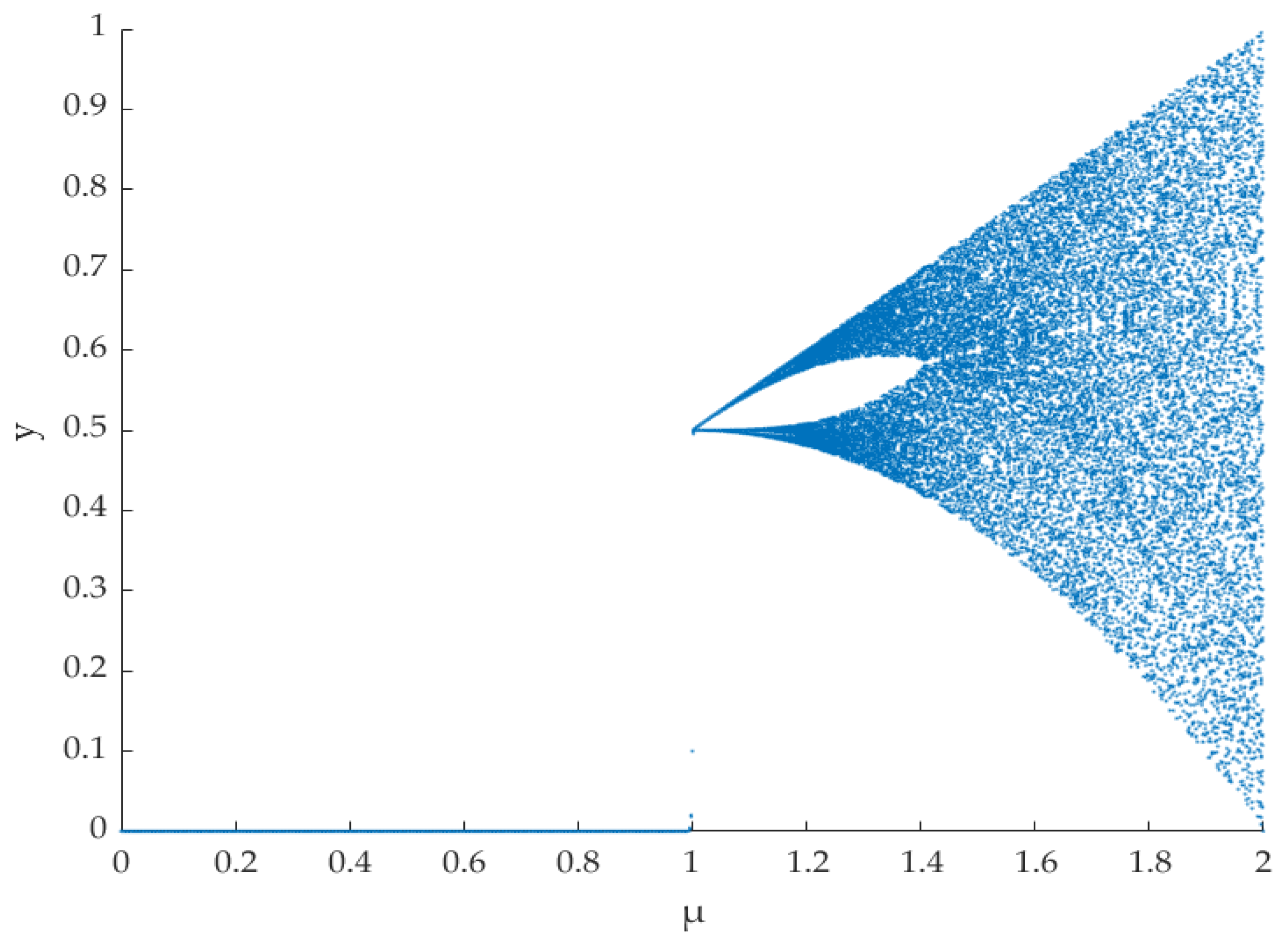
Figure 2.
Chaotic tent map Lyapunov exponential.
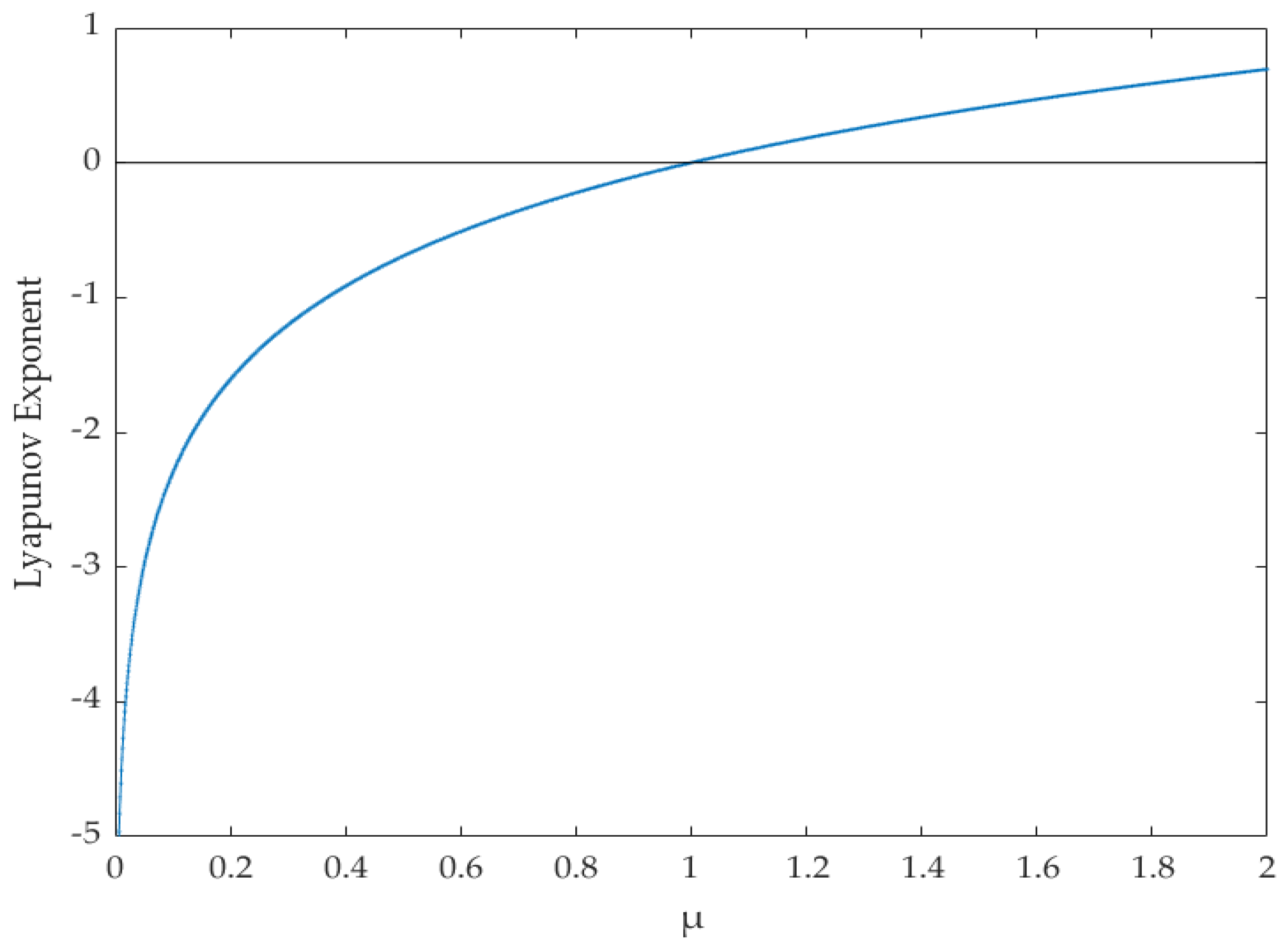
Figure 3.
Probability density maps of Cauchy distribution, t-distribution and Gaussian distribution.
Figure 3.
Probability density maps of Cauchy distribution, t-distribution and Gaussian distribution.
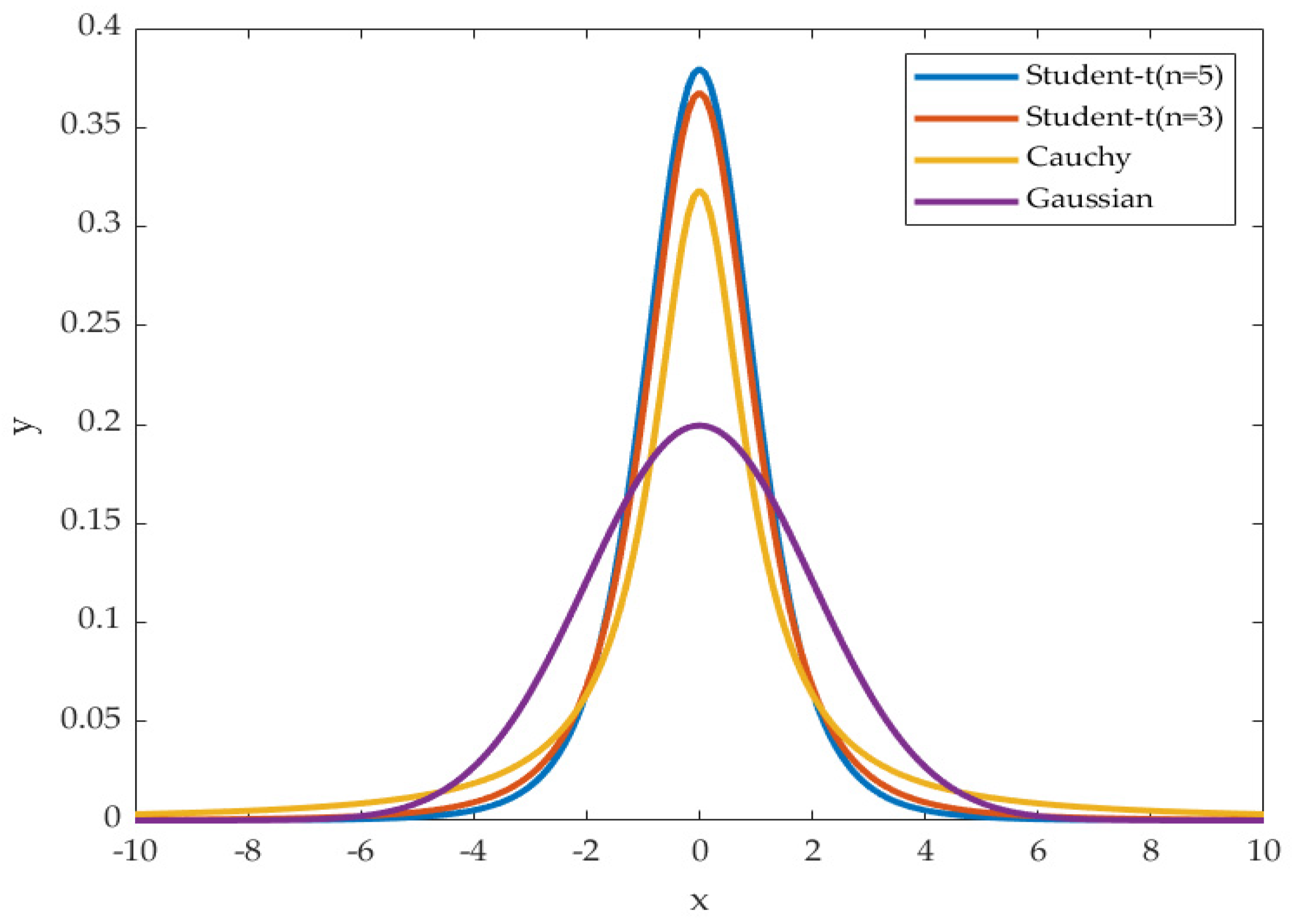
Figure 5.
Deployment of each algorithm node.
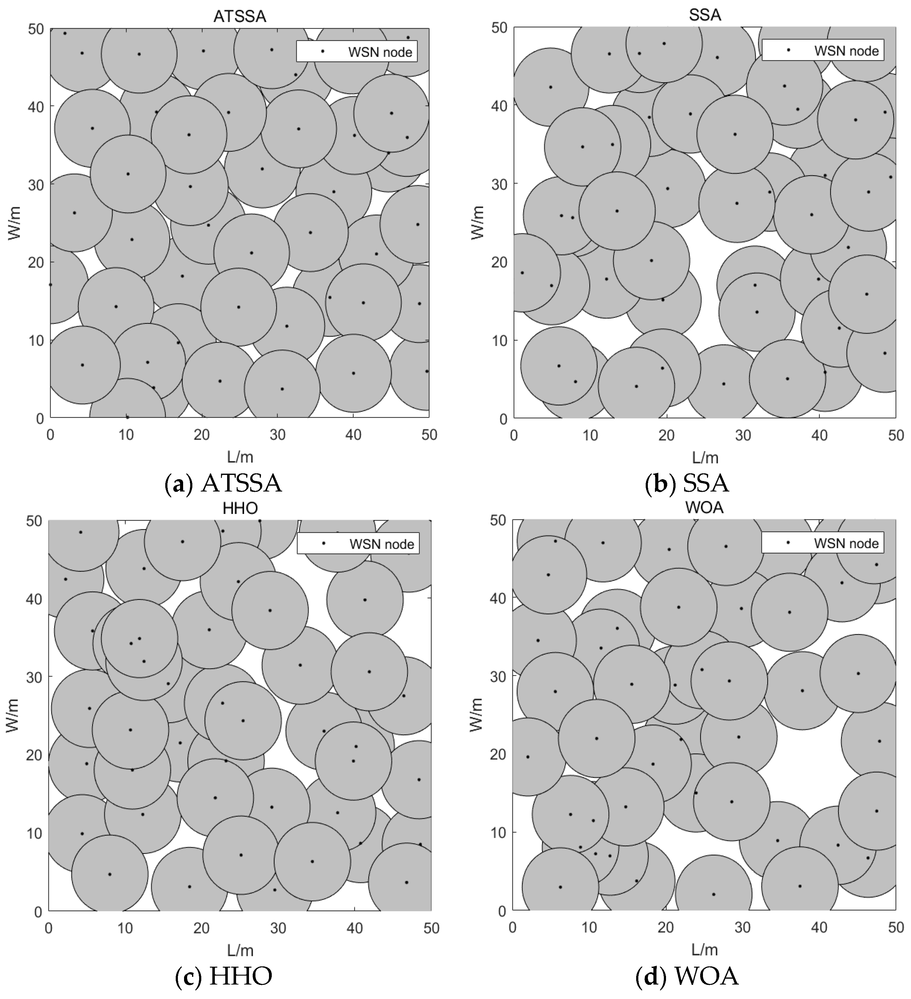
Figure 6.
Comparison of average coverage rate.
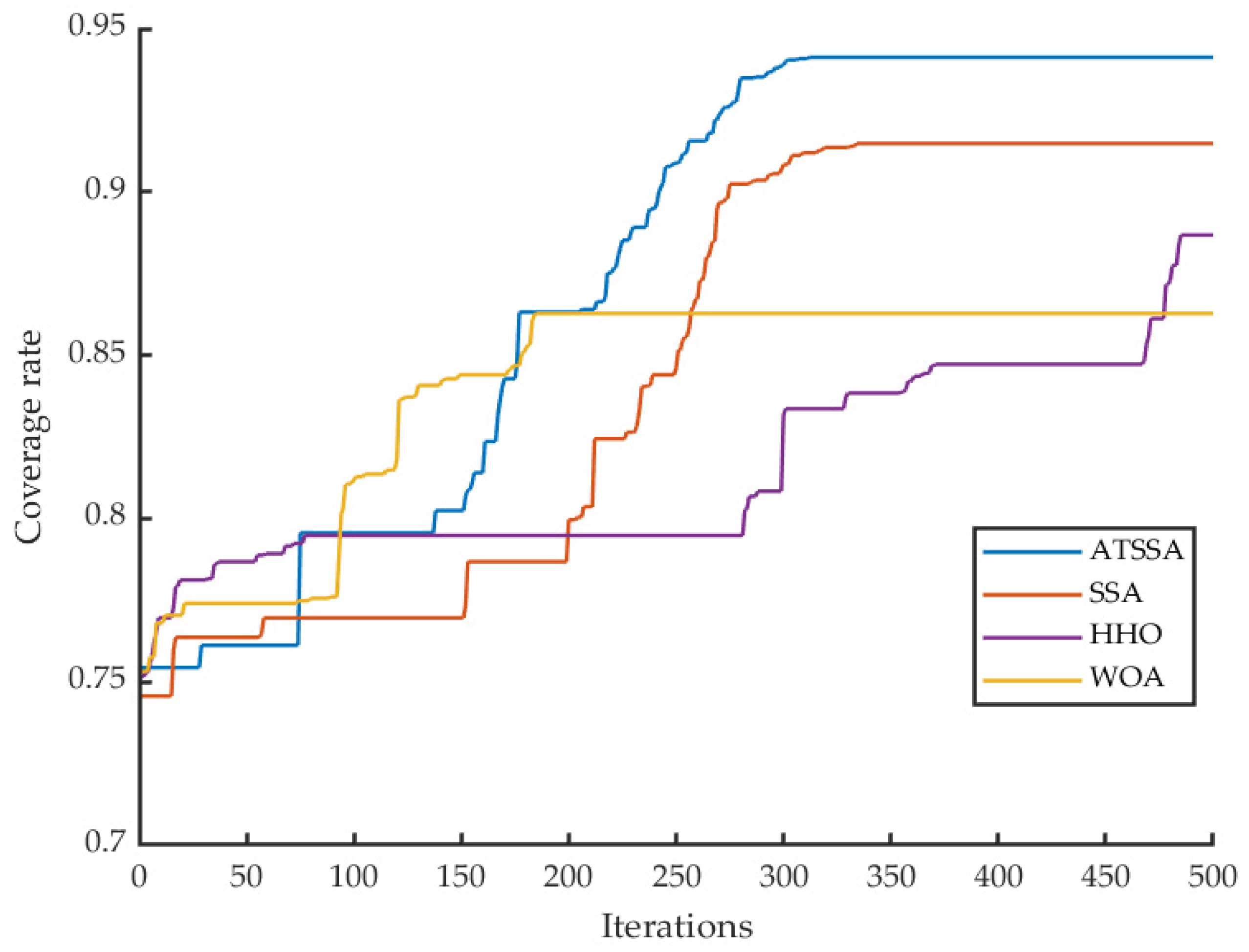
Figure 8.
Comparison of average coverage rate.
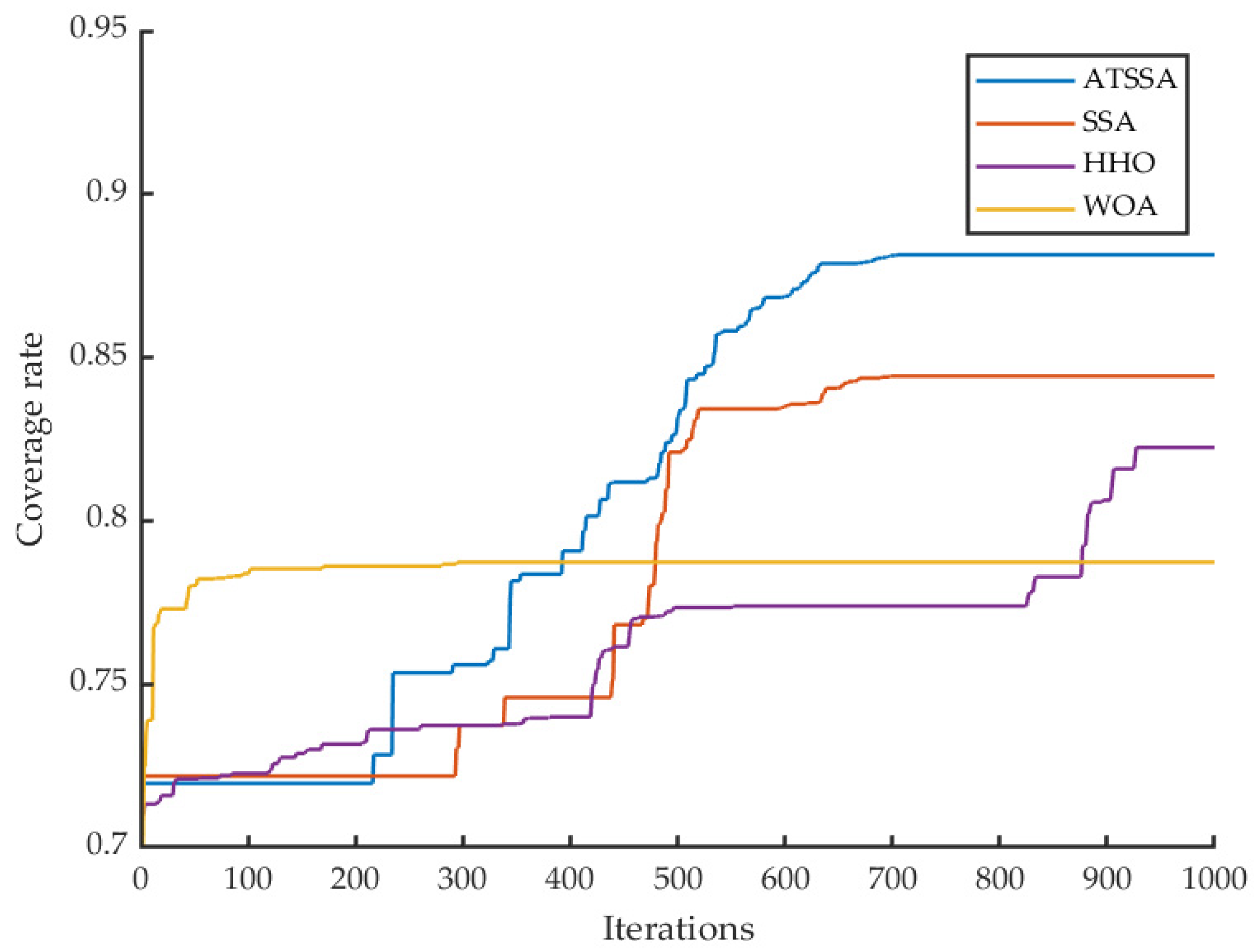
Figure 9.
Number of nodes required and specific coverage.
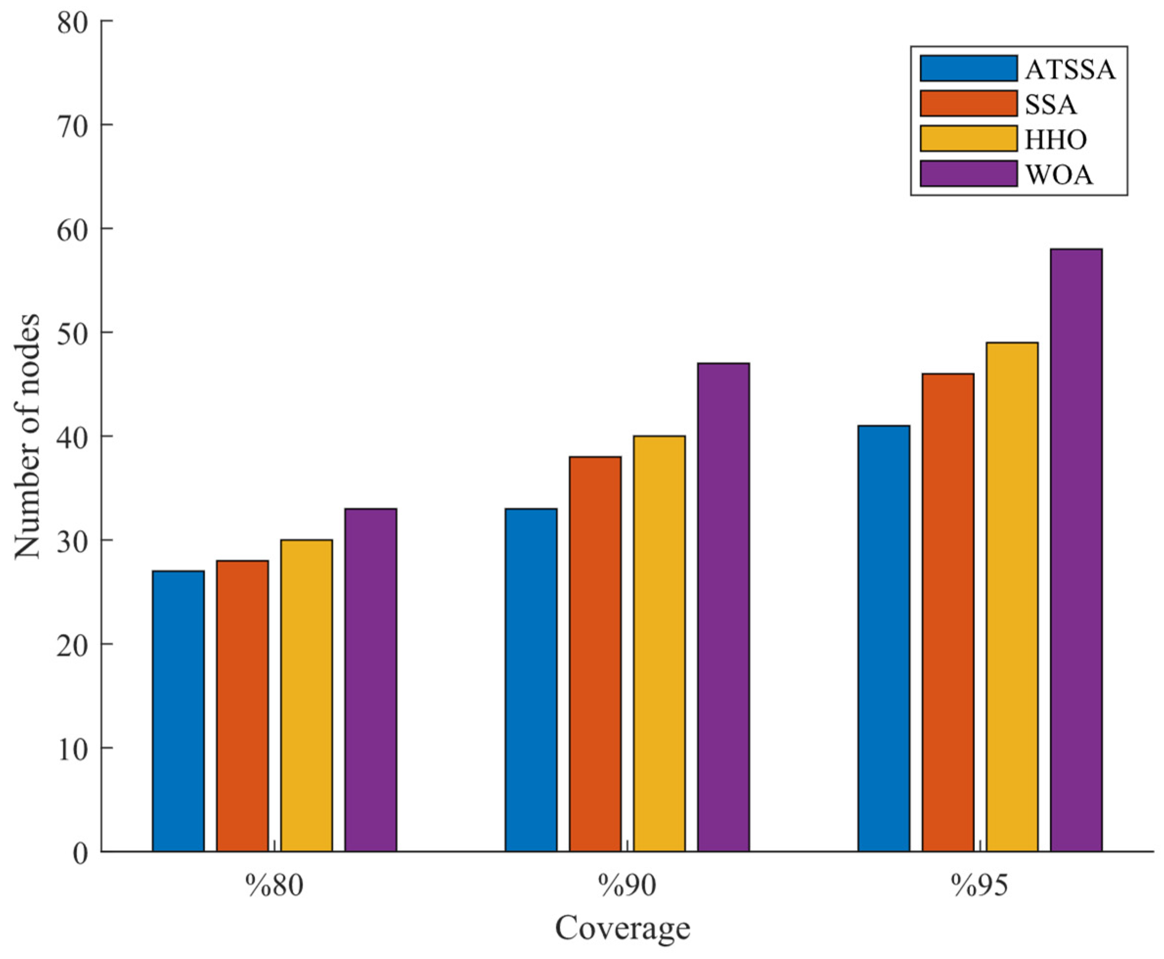
Table 1.
The parameters used in the algorithms.
| Algorithms | Parameters | Values |
| ATSSA |
|
|
| SSA |
|
|
| HHO |
|
|
| WOA |
|
|
Table 3.
Comparison of average coverage rate.
| Num | ATSSA | SSA | HHO | WOA |
| 1 | 0.9304 | 0.9228 | 0.8744 | 0.8424 |
| 2 | 0.9424 | 0.9292 | 0.8904 | 0.8044 |
| 3 | 0.9480 | 0.9112 | 0.9028 | 0.8564 |
| 4 | 0.9296 | 0.9180 | 0.8928 | 0.8336 |
| 5 | 0.9312 | 0.8884 | 0.8784 | 0.8492 |
| 6 | 0.9332 | 0.9224 | 0.8628 | 0.8764 |
| 7 | 0.9352 | 0.9152 | 0.8848 | 0.8244 |
| 8 | 0.9288 | 0.9336 | 0.8940 | 0.8492 |
| 9 | 0.9268 | 0.8936 | 0.8780 | 0.8360 |
| 10 | 0.9184 | 0.9264 | 0.8752 | 0.8360 |
Table 5.
Comparison of average coverage rate.
| Num | ATSSA | SSA | HHO | WOA |
| 1 | 0.8786 | 0.8494 | 0.8388 | 0.8000 |
| 2 | 0.8698 | 0.8443 | 0.8304 | 0.8018 |
| 3 | 0.8853 | 0.8192 | 0.8327 | 0.7935 |
| 4 | 0.8908 | 0.8694 | 0.8208 | 0.7788 |
| 5 | 0.8739 | 0.8671 | 0.8176 | 0.8133 |
| 6 | 0.8869 | 0.8437 | 0.8267 | 0.7863 |
| 7 | 0.8939 | 0.8453 | 0.8359 | 0.7643 |
| 8 | 0.8643 | 0.8502 | 0.8394 | 0.8273 |
| 9 | 0.8620 | 0.8498 | 0.8261 | 0.7682 |
| 10 | 0.8739 | 0.8467 | 0.8298 | 0.7796 |
Table 7.
Comparison of number of nodes.
| Coverage Rate | ATSSA | SSA | HHO | WOA |
| 80% | 27 | 28 | 30 | 33 |
| 90% | 33 | 38 | 40 | 47 |
| 95% | 41 | 46 | 49 | 58 |
Disclaimer/Publisher’s Note: The statements, opinions and data contained in all publications are solely those of the individual author(s) and contributor(s) and not of MDPI and/or the editor(s). MDPI and/or the editor(s) disclaim responsibility for any injury to people or property resulting from any ideas, methods, instructions or products referred to in the content. |
© 2023 by the authors. Licensee MDPI, Basel, Switzerland. This article is an open access article distributed under the terms and conditions of the Creative Commons Attribution (CC BY) license (http://creativecommons.org/licenses/by/4.0/).
Copyright: This open access article is published under a Creative Commons CC BY 4.0 license, which permit the free download, distribution, and reuse, provided that the author and preprint are cited in any reuse.


