
Submitted:
24 October 2024
Posted:
24 October 2024
You are already at the latest version
Abstract
To address the issue of low prediction accuracy for sub-grid scale turbulence-radiation interaction (SGS-TRI) characteristics, which impacts the precision of remote infrared signal calculations for gas jet, a term for correlation of radiation-participating component fluctuations with temperature fluctuation was introduced into the current sub-grid Snegirev equation; Simultaneously, we established a new method that is more convenient in complex projects for solving the dynamic sub-grid model coefficients, e.g., dynamic Smagorinsky model and temperature variance model. The validity of these algorithms was confirmed through direct numerical simulations (DNS) for isotropic turbulence and test data of high-temperature air jet flow. The Multi-Scale Multi-Group Wide-Band (MSMGWB) k-distribution model was used to calculate radiative transfer in strongly non-isothermal and inhomogeneous media such as the remote infrared sensing of jet plume scenario considering influences of TRI and SGS-TRI. The study for axisymmetric jet plume revealed that the TRI accounts for more than 1/3 of total remote infrared signal in the 3-5micron band, with the SGS-TRI effect contributing more than 10%. Additionally, this influence was found to further increase with increasing detection distances.
Keywords:
Infrared radiation
; Remote sensing
; Turbulence-radiation interaction
; Gas jet
; SGS-TRI
1. Introduction
The phenomenon of turbulence-radiation interaction (TRI) is pronounced in high-temperature turbulent gas jet. Turbulence induces fluctuations in temperature, composition and pressure of the non-uniform gas jet, which subsequently causes the fluctuations of local radiation absorption coefficient and the Planck function for radiation emission. These result in variations in internal radiation transmission and can even affect the fluctuations of radiation heat transfer, thereby influencing the turbulent flow of gas jet [1]. Notably, the gas radiation absorption coefficient and the Planck function for radiation emission are nonlinear functions of temperature. This nonlinearity leads to a significant disparity between the time-averaged characteristics of transient radiation of turbulent gas and the radiation characteristics of its time-averaged flow field. In many scientific contexts, particularly in engineering applications, the former is often more relevant. For instance, a collaborative study by Modest and Haworth examined the TRI characteristics of methane-air axisymmetric diffusion flames [1]. Their findings indicated a 150 K difference in the maximum flame temperature when TRI was considered compared to when it was not, as well as a sixfold variation in nitric oxide production. Furthermore, as current optical characteristic recognition algorithms evolve towards three-dimensional space-time domain, the fluctuating characteristics of infrared radiation from gas jets, driven by turbulence [2], are anticipated to emerge as significant target features for hydro-carbon fuel aircraft.
Most research of TRI has been conducted in the field of combustion. As early as the 1980s, the probability density function (PDF) method based on Reynolds-averaged Navier-Stokes equations (RANS) emerged [3,4]. The Snegirev method [5] emerged at the beginning of this century. Its fundamental concept involves expressing the fluctuation characteristics of the emission term in the radiative transfer equation (RTE) as a function of the local temperature fluctuation variance. Subsequently, this method allows for the determination of temperature fluctuation within the RANS flow field by establishing a specialized transport equation for variance distribution. The aforementioned TRI characteristic calculation method based on RANS is still under development [6,7]. However, due to the inability to model the fluctuation of absorption term of the radiative transfer equation, this method can only be used in the scenario meeting the optically thin fluctuation approximation (OTFA) [7], which restricts its applicability in many engineering contexts.
This article focuses on the gas-free jet, where the turbulent fluctuation scale at a distance from the nozzle outlet is comparable to the nozzle diameter, which does not conform to the OTFA assumption. The practical calculation of its TRI characteristics can only be addressed through the radiative transfer equation of the transient turbulent flow field, derived from large eddy simulations (LES). Blunck et al. conducted a numerical study on the TRI characteristics of the jet in the 4.3micron band for an exhaust system equipped with a pre-swirl device [8]. They discovered that turbulent fluctuation minimally affects the radiation emitted from the core area of the jet; however, at distances from the nozzle exit or in proximity to the jet mixing layer, turbulent fluctuation significantly impacts the time-averaged radiation. The fluctuating radiation characteristics of the gas jet exhibit many similarities to those of flames and when the Reynolds number is sufficiently high, these characteristics are not sensitive to variations in the Reynolds number. Additionally, computational study of Damien et al on the TRI characteristics of radiative heat transfer in a rectangular combustion chamber with a triangular flame stabilizer [9] revealed that the effects of temperature autocorrelation fluctuation, temperature and absorption coefficient correlation fluctuation and absorption coefficient autocorrelation fluctuation on flame emission radiation fluctuation are all substantial and cannot be overlooked. Notably, none of the aforementioned LES-based calculations account for the influence of sub-grid scale turbulence fluctuations on TRI characteristics. The Coelho team employed direct numerical simulation (DNS), ray tracing and narrow-band k-distribution models to evaluate the SGS-TRI characteristics of isotropic turbulence and free jets [10,11]. Their findings indicate that the impact of SGS-TRI on the emission term of the radiative transfer equation is significantly greater than that on the absorption term. Furthermore, they observed that as optical thickness increases, temperature fluctuations intensify, leading to a higher proportion of SGS-TRI in the overall radiation; specifically, when the optical thickness is 1, the proportion of SGS-TRI ranges from 13% to 25%. Additionally, the influence of SGS-TRI on the radiative transfer of free jets is primarily concentrated at the edge of jet, where the overall radiant brightness is minimal. Notably, the variation in radiant brightness calculations due to the consideration of sub-grid scale fluctuations in radiative transfer can exceed one-third. In the context of flame radiation heat transfer, the filtered density function (FDF) method [12], which is based on the probability density function (PDF) method, is pre-dominantly used to assess SGS-TRI characteristics. The results indicate that SGS-TRI is significantly influenced by factors related to sub-grid scale chemical reactions and temperature fluctuations. In flames with large optical thickness, the contribution of SGS-TRI to radiant heat is considerably greater than that observed in gas jets, it can even surpass the contribution from turbulent fluctuations at a resolvable scale [13,14,15].
As the significance of SGS-TRI became increasingly apparent, Poitou et al. proposed a modeling method in 2007 [16]. This method extends the previously mentioned Snegirev method into large eddy simulations by using the same expression of emission term fluctuation in the RTE against gas temperature fluctuation, combined with a sub-grid scalar variance model [17]. The Coelho team assessed the accuracy of this modeling method in gas radiative heat transfer calculation for a simple axisymmetric flame, using the FDF model as benchmark [18]. The results indicate that the existing sub-grid Snegirev expression significantly underestimates the emission term fluctuation in flame RTE. Additionally, the fixed coefficient sub-grid scalar variance model considerably underestimates the sub-grid temperature fluctuations. Consequently, the combined effect of these two factors leads to the predictions of the SGS-TRI characteristics of diffusion flames being considerably lower than the actual measurements.
Current research on TRI primarily examines its influence on narrow-band infrared signals used in non-contact measurement for flow field and on full-spectrum radiative heat transfer, which have different characteristics [19]. However, no published research has addressed the TRI and SGS-TRI characteristics of gas jet as well as their modeling methods for the atmospheric infrared window wide-bands, which are pertinent to the field of remote sensing (e.g., 3-5 micron and 8-14 micron band). This paper employs a Multi-Scale Multi-Group Wide-Band k-distribution model [20,21] (Section 2.1) to calculate the TRI characteristics for remote infrared signals of axisymmetric gas jets in the 3-5 micron wave band. It also demonstrates that the model can effectively perform radiative transfer calculations in scenarios where the correlation-k characteristic of the gas absorption spectrum is notably disrupted due to substantial differences in temperature and composition between the combustion gas and the ambient air as well as strong thermodynamic state parameter inhomogeneities in their mixing layer (Section 3.3).To address the low prediction accuracy of existing SGS-TRI models, this study introduces a term describing correlation between combustion gas species concentration and temperature fluctuations into the sub-grid Snegirev relationship (Section 2.2). Furthermore, a new ensemble average calculation method, which is more applicable in complex engineering contexts, is developed to resolve the coefficients of dynamic Smagorinsky model and temperature variance model (Section 2.3). The validity of these algorithms is confirmed through DNS calculations of isotropic turbulence (Section 3.1) and comparison with measurement data of high-temperature air jet flow field (Section 3.2). Based on these, the TRI and SGS-TRI characteristics of 3-5micron band infrared signal from an axisymmetric combustion gas jet at different detection distances are analyzed (Section 4.1), and the characteristics of the MSMGWB model are employed to elucidate the formation mechanism of the observed phenomena (Section 4.2).
2. Radiation Transfer Equation Based on k-Distribution Model for Solvable Scale Turbulent Flow Field
2.1. MSMGWB Model
For the 3-5 micron band infrared radiation emitted by combustion gases without particles and attenuated by ambient air before reaching optical detectors, the RTE (without considering gains from ambient air) can be written as [20,21]
where, is the wave number, and are the spectral extinction coefficient and the spectral scattering coefficient at wave number , respectively. is the thermodynamic state parameters of the mixed medium that affect and (comprising gas species mole fraction , pressure and temperature ), the spectral radiance, the blackbody’s spectral radiance at and the location along the radiation transfer path. In this work, , where is the spectral absorption coefficient of n-th species, and subscript denote water vapor, carbon dioxide, carbon monoxide and aerosol particles, respectively. The values of were obtained from the LBL approach based on HITEMP database (2010 version) [22], and the values of and were calculated using Mie scattering theory [23,24]. All the parameters will be based on the local unless otherwise indicated.
In hot combustion gas remote detection scenario, water vapor and carbon dioxide are treated as participation in both emission and absorption process, while carbon monoxide and aerosols only contribute to the attenuation part, because they exist only in the atmosphere rather than in turbo gas. Besides, the emission and scattering gain from atmosphere are not considered here since they are commonly treated as background radiation and calculated separately. Therefore, based on its linearity, Equation (1) can be rewritten as [19,21,25],
where results from the emission of H2O or CO2, but is subject to the absorption of both in combustion gases and the absorption and scattering of all four species in atmosphere.
The MSMGWB model employs a method of grouping spectral absorption coefficients to address the significant differences in temperature and composition between combustion gas and ambient air. These differences result in a lack of correlated-k characteristics in absorption spectra, which significantly reduces the calculation accuracy of conventional k-distribution models. The principle is to allocate the spectral subintervals, which are dominated by 'cold absorption lines' and 'hot absorption lines', into different subset, ensuring spectral absorption coefficients within each subset have similar thermodynamic state parameter dependences, i.e., exhibit correlated-k characteristics under the concerned gas thermodynamic state parameter combinations, as illustrated in [20].
By performing independent k-distribution transformations for each spectral subset, the final radiative transfer equation of the MSMGWB model is [20],
where, , , and represent the emission coefficient, absorption coefficient, stretching coefficient and blackbody radiance, respectively, corresponding to the jth radiative transfer equation of MSMGWB model.
The reliability of MSMGWB model in remote sensing scenario is preliminary validated through two types of 1D cases, as sketched in Figure 1, using calculation results of line-by-line (LBL) approach as benchmark. The results shown in Figure 2 and Figure 3. indicate that MSMGWB model can almost perfectly deal with radiation transfer in gases with temperature, participating component mole ratio, as well as pressure inhomogeneities and v aerosols with various sizes and components. Where radiation characteristics of various aerosols were calculated by Mie theory [26,27]. More calculation results of the MSMGWB model in the 1D cases can be found in reference [21].
2.2. Dynamic Smagorinsky Model Based on Relaxation Factor
The governing equations of the solvable scale flow field can be derived by filtering the NS equation, so the governing equations of large eddy simulation can be obtained as follows,
where, ,,,,,andare represent density, velocity, pressure, mass fraction of each component, total energy per unit mass of fluid, total enthalpy per unit mass of fluid, and subgrid-scale stress, respectively.
Where,
where, ,,andare represent specific heat ratio, universal gas const, specific heat at constant pressure, and diffusion coefficient, respectively.
In equations (4)-(16), the superscript "-" denotes the volume-averaged quantity within a cube with characteristic side length , termed the "filtering length". The superscript "~" signifies the Favre average. In equations (4)-(7), there exist unclosed terms, i.e. the sub-grid terms, that require modeling for closure. This paper employs the Smagorinsky sub-grid model:
When applying dynamic Smagorinsky model of Lilly [28], the calculation method for is as follows,
Here, denotes a filtering scale larger than . The superscript '^' signifies the volume-averaged value of this parameter within a cube with characteristic side length , while the superscript indicates the Favre average at this scale.
In equation (21),
denotes the ensemble average. For two-dimensional flows, the ensemble average of equation (21) can be spatially averaged in statistically homogeneous directions. However, in complex three-dimensional flows, there are no statistically homogeneous directions, preventing the use of spatial averaging to calculate dynamic eddy viscosity coefficients. The direct temporal averaging method proposed by Meveneau is computationally expensive due to excessive memory requirements; whereas the fluid particle averaging trajectory method necessitates solving additional transport equations, which is complicated and has low computational stability [29]. To enhance the applicability of both the dynamic Smagorinsky model and temperature variance model in Large Eddy Simulation (LES) calculations for complex three-dimensional flow fields, this paper establishes an ensemble averaging calculation method based on relaxation factors () as follows (using an arbitrary variable as an example):
here,, is serial number of calculation time step, and denotes current time step. This algorithm eliminates the need to solve additional transport equations and only requires the storage of values on each computational grid, thus resulting in minimal memory requirements.
2.3. Improved SGS-TRI Model
Applying a box filter to equation (3) in the same manner, we obtain the following equation,
Extensive research indicates [30,31] that when the filter scale is optical thin, the SGS-TRI characteristics of its absorption term are not pronounced. As a result, equation (25) can be reformulated as follows,
For the first term on the right-hand side of the equation (26), based on the method proposed by Snegrive [5], expanding it in the Taylor series and neglecting higher-order terms yields,
By setting and in equations (27), we can obtain the filtered radiative transfer equation:
where andare terms to be modeled. The latter can refer to the subgrid-scale scalar variance model by Pierce and Moin [17]:
the model coefficient can also be determined based on Lilly's dynamic model [28].
The ensemble average in equation (30) is also calculated using the method proposed in section 2.1, namely equation (24). It is noteworthy that the impact of the term in equation (28) is neglected in the existing subgrid-scale Snegirev method [5]. However, turbulence theory and extensive DNS simulation results have confirmed a strong correlation between fluctuations in component concentration () and local temperature fluctuations within chemically frozen turbulent mixing layers [32] (see section 3.1.4). Furthermore, since , in most cases, the existing subgrid-scale Snegirev method underestimates the influence of subgrid-scale turbulent fluctuations on the emission terms of the RTE. The term in equation (28) can be estimated based on local components and temperatures at different times by fitting their slope using least squares. Following a principle similar to that used for equation (24), wherein higher weights are assigned to current time and lower weights to more distant time, we obtain,
3. Verification of Model Calculation Accuracy
This section, the reliability of the relaxation factor-based methods to solve coefficients of dynamic Smagorinsky model and SGS temperature variance model was verified using DNS for compressible isotropic turbulence flow, which was also used to assess the relevance between species concentration fluctuations and local temperature fluctuations in turbulent mixing layers as well as rationality of incorporating term within the SGS-TRI model. Additionally, by comparing the results of hot air free jet LES calculations with experimental data, the accuracy of the dynamic Smagorinsky model based on relaxation factors was further validated.
3.1. DNS for Decaying Isotropic Turbulence
3.1.1. Verification of DNS Method
Direct numerical simulations of compressible isotropic turbulence serve as a prime example for testing the resolution of small-scale fluctuations. This paper selects a computational case [33] involving isotropic turbulence with an initial Taylor-Reynolds number and an initial turbulent Mach number , which decays under the influence of viscosity. The computational domain is , and the number of grids is 2563. Convective terms are computed using the TENO-5 scheme [34], while viscous terms are discretized using a sixth-order central difference scheme. Time advancement is achieved through a TVD-type three-step third-order Runge-Kutta method [35], with a time step of 0.001s and a calculation duration of 3.5 times the large eddy turnover time . The initial field conditions assume that the energy spectrum satisfies equation (34) and that the divergence of both velocity and temperature fields is zero.
where, is the wave number, is the wave number at the peak of the wave, and A is a constant value used to determine the specified initial turbulent kinetic energy. In this paper, the value is taken as .The calculation methods for turbulence statistics such as the Taylor scale Reynolds number, turbulent kinetic energy, turbulent Mach number, velocity derivative skewness, and large eddy turnover time are as follows,
where,
After the flow field development time exceeds one large eddy turnover time, it can be considered that it is no longer affected by the initial conditions. As shown in Figure 4, the time evolution of the Taylor-scale Reynolds number, turbulent kinetic energy, turbulent Mach number, and root mean square of the normalized density in this article are in good agreement with the data from Samtanery [33]. The velocity derivative skewness is a high-order statistic that is very sensitive to small-scale motion in the flow field. The TENO-5 scheme reacts well to the development trend of this quantity, and the peak and valley are calculated.
.
3.1.2. Coefficient Verification for Dynamic Smagorinsky Model Based on Relaxation Factor
Scale filtering () is applied to the aforementioned DNS data. Here, represents the grid scale of the DNS computation, while denotes the filtering scale. When takes values of 4, 8, 16, and 32, the subgrid-scale energy accounts for 5%, 15%, 40%, and 70% of the total turbulent kinetic energy, respectively. Subsequently, is employed for calculating equation (21). As illustrated in Figure 5, for and , the dynamic Smagorinsky model coefficients solved by the relaxation method are very close to the theoretical value 0.0384 (the notation 4-8 indicating and ).
3.1.3. Correction of Temperature variance model coefficient
Based on the aforementioned DNS data, Figure 6 presents the time evolution curves for the coefficients of the dynamic temperature variance model calculated at different filtering scales, as well as the correlation coefficients between the calculating values and true values of temperature variance.
It can be observed that the calculated sub-grid temperature variance model coefficients stabilize at 0.1, 0.2, and 0.6 for the three different filtering scales. This indicates that the coefficients are significantly influenced by the filtering scale, making it unsuitable to use a fixed coefficient model for parameterization. Furthermore, the values of reported in reference [28] are considerably lower across various filtering scales. The correlation between the true sub-grid temperature variance and the values predicted by the dynamic model is quite strong, reaching 0.9 and 0.7 at filtering scales for and (when , the reconstruction rate of turbulent kinetic energy falls below the fundamental requirements for LES), thereby demonstrating the accuracy of this parameterization method.
Figure 7 and Figure 8 display the variations of the true values of dimensionless sub-grid temperature variance and the predicted values from the dynamic model over time and filtering scales. It is evident that, when and , the modeled values closely align with the true values as time changes, with a notable discrepancy only at larger filtering scales (). This demonstrates the accuracy of the parameterization method within the scales of interest for large eddy simulations.
(left) and the correlation coefficient (right) at different filtering scales.
, the variation of the dimensionless sub-grid temperature variance (true values) and the calculated values from the dynamical temperature variance model across different filter scales.
3.1.4. Verification and Analysis of the Correlation Between Gas Components and Temperature
To examine the correlation between gas component fluctuations and temperature fluctuations in chemically frozen turbulent flow fields, thereby to verify the rationality of adding term in the Snegirev SGS-TRI model, the were calculated based on the DNS data from compressible isotropic turbulence flow field, as shown be follow,
The time evolution of at different filter scales are shown in Figure 9. It is evident that, at various filter scales, both the component fluctuations and temperature fluctuations exhibit a very high degree of correlation. When , the correlation between the two is even higher than the direct numerical simulation (DNS) results. This can be attributed to the filtering out of certain small-scale fluctuations, which enhances the correlation. At the scales of interest in large eddy simulation (LES), namely and , the correlation remains at a high level, around 0.99 and 0.97 respectively. This supports the rationale for including the term in the SGS-TRI model to establish Eq. (28).
3.2. LES for High Temperature Air Jet Flow
The axisymmetric convergent nozzle has an outlet diameter of 50.8 mm, with a nozzle pressure ratio (the ratio of jet stagnation pressure to ambient pressure) of 1.357 and a static temperature ratio of jet at the nozzle outlet to the ambient temperature of 1.764. The ambient temperature is 288 K and the pressure is 101,325 Pa. The total grid number used in the LES computation was about 10 million, achieving a reconstruction rate of turbulent kinetic energy about 93%. The resulting instantaneous Mach number and temperature contour at jet symmetry plane are presented in Figure 10. The iso-surface of vorticity colored with local temperature is shown in Figure 11. The vorticity is caculated by criterion, as Equation (44). Furthermore, the calculated jet velocity field is compared to the PIV data from Bridges and Wernet [36], while the temperature field is validated against the rotating Raman scattering results from Locke et al. [37] and the Rayleigh scattering results from Mielke et al. [38], as shown in Figure 12 and Figure 13. Here, denotes the radial position, specifies the diameter of the jet outlet, indicates the velocity at the center of the jet outlet, represents the temperature at the center of the jet outlet, refers to the temperature of the ambient air, and signifies the turbulent kinetic energy of the jet.
The numerical results obtained from the large eddy simulation presented in this paper accurately capture the turbulent fluctuation characteristics of the hot jet, as well as the flow direction and spanwise decay characteristics of the jet in the surrounding air. Given that the size and Reynolds number of the jet in this case are relatively small, the results of the large eddy simulation exhibit considerable sensitivity to the sub-grid eddy viscosity model. The dynamic Smagorinsky model, which is based on a relaxation factor developed in this study, effectively addresses these requirements. The differences between the calculated results of turbulent kinetic energy distribution along the axis and the experimental data may stem from the difference between the Favre-averaged value of turbulent kinetic energy output by the sub-grid model and its ensemble average.
4. Analysis of TRI Characteristics of Axisymmetric High-Temperature Gas Jet
4.1. Verification of Infrared Radiation Characteristic Calculation for Combustion Gas Jet
The calculation of the infrared radiation characteristics of an axial combustion gas jet in the 3-5micron band presented in case1 of this section is still based on the convergent nozzle described in Section 3.2, the only difference is to replace the jet medium by combustion gas. This adjustment takes into account the influence of the effect of real gas, resulting in a gas jet length that is slightly longer than that of the air jet. Case 2 has higher gas temperature, which is regulated through the combustion of aviation kerosene at varying equivalence ratios, simultaneously adjusting its components. Additionally, the nozzle size is enlarged to maintain the Reynolds number consistent with that of case 1, as detailed in the table below.

Table 1.
Parameters of LES cases.
| Case 1 | Case 2 | |
| Diameter of nozzle outlet/mm | 50.8 | 97.2 |
| Total temperature/K | 554.62 | 794.65 |
| Total pressure/Pa | 137498 | |
| Ma | 0.67 | |
| Mass fraction of oxygen | 20.85% | 18.63% |
| Mass fraction of water vapor | 0.79% | 1.54% |
| Mass fraction of carbon dioxide | 2.05% | 3.98% |
| Mass fraction of carbon monoxide | 0.000015% | 0.000015% |
The ambient air is set to the equatorial mode in the MODTRAN 5.0 software (where the mass fraction of water vapor and carbon dioxide are1.44%and 0.06%, respectively, meaning the proportion of radiation participating components is completely different from that of the combustion gas jet), and the aerosol is set to the sea surface mode with 23km visibility. The extinction efficiency of aerosols in 3-5 micron band is shown in Figure 14. The infrared detection direction is perpendicular to the jet axis, and the detection distances are set to 0.2, 3.0, and 45km, respectively. For each physical time step, flow field LES is performed (computation time is about 1.1 seconds on a single computing node with 256-cores/512-threads), followed by an infrared imaging calculation for the entire flow field (computation time is about 0.4 seconds). Figure 15 shows the instantaneous infrared imaging and infrared radiance calculation error distribution of case 2 at a certain moment under 45km detection distance where the radiance error distribution of MSMGWB model is calculated by contrasting with results of the line-by-line model [39] (requiring approximately 6 hours of computation time) ignoring the influence of SGS-TRI. The error is found to be within 8%. This demonstrates that the MSMGWB model is adept at long-range radiative transfer computations in scenarios characterized by substantial disruptions of correlated-k characteristics of absorption spectra, stemming from inhomogeneities of gas temperature and composition.
4.2. TRI Characteristic Analysis for High Temperature Combustion Gas Jet
Figure 16 and Figure 17 illustrate 3-5micron band infrared images for case 2 at various distances derived by ray-trace [21] based on the time-average flow field (i.e., ignoring TRI effect) and the instantaneous flow fields followed by time-averaging. The latter has longer core areas and exhibits higher maximum radiance compared to the former. The gas jet infrared signal detected by the actual infrared detector is clearly the latter.
Figure 18 illustrates the distribution of percentage increases in 3-5micron band infrared image, attributed to TRI for case 2 at 0.2 km detection distance. It is evident that flow field fluctuation significantly affects infrared radiation, especially in the violent turbulent regions of gas-ambient mixing layer. Conversely, in the core area characterized by high temperature and high radiance, the TRI impact is relatively small, especially near the center of nozzle exit, which aligns with the findings presented in the literature [8]. Radiation intensity of pixels in the infrared images corresponding to various positions of combustion gas jet at 0.2 km detection distance is shown in Figure 19. Figure 20 illustrates the time evolution curve of the integrated radiation intensity of the whole image. The normalized fluctuation of the integrated radiation intensity is defined as follows,
The relative amplitudes and frequencies of radiation intensity of each pixel are very high, but the integral of them has much lower relative amplitude and frequency, causing by canceling one another’s fluctuation.
Figure 21 and Figure 22 illustrate the percentage influence of TRI/SGS-TRI on the integrated radiation intensity of the jet at various detection distances. Notably, the effect of component fluctuation in SGS-TRI is determined by excluding the term in equation (28).
The two figures illustrate that, at various jet temperatures, the TRI accounts for more than 1/3 of the total infrared signal, with its influence further amplifying as the detection distance increases. Among the effects of TRI, the resolvable scale TRI plays a dominant role; however, the contribution of SGS-TRI is also significant, accounting for over 10% of the total infrared signal of the jet, which corresponds to approximately 50% of the contribution from the resolvable scale TRI. This finding is consistent with the proportions of SGS-TRI reported in the literature based on DNS studies of chemically frozen free jet [10,11]. Within the SGS-TRI effect, the contribution from component fluctuation is approximately one-third, underscoring its importance.
To analyze why the influence of TRI on the jet infrared signal increases with detection distance, Figure 23 presents the temperature dependences of emission coefficients and corresponding atmospheric transmittances for RTE’s with a significant contribution ratio (W) to at various detection distances, their cumulative contribution ratio accounts for approximately 90%. For clarity, the minimum transmittance is set at no less than .
At shorter transmission distances, where the atmospheric attenuation is minimal (red line in the right part of Figure 23), the combustion gas radiation spectrum is mainly contributed by the cold absorption lines of water vapor and carbon dioxide, their corresponding values vary slowly with temperature increasing. Conversely, at longer transmission distances, the emitted radiation from the cold absorption lines of combustion gas is almost entirely absorbed by the same cold lines of water vapor and carbon dioxide in low-temperature atmosphere (blue line in the right part of Figure 23). As a result, the remaining infrared signals predominantly originate from hot absorption lines in the combustion gas, which abilities of radiation absorption (red line in the left part of Figure 23) and emission are very weak at low temperature states, but exhibiting a rapid increase with temperature increasing (high value). Consequently, temperature fluctuations in turbulence flow induce a more pronounced positive correlation between and for the spectrum consisted of the hot absorption lines compared to that of cold absorption lines. This ultimately results in an increased relative contribution ratio of TRI as detection distance increases.
5. Discussion and Conclusions
This paper employs LES and a MSMGWB k-distribution gas radiation model to investigate the effects of high-temperature combustion gas jet turbulence fluctuation on its remote infrared radiation characteristics within the 3-5micron band. To address the issue that existing algorithms significantly underpredict the SGS-TRI, we introduced a term related to the correlation between fluctuations of radiation-participating components and temperature into the SGS Snegirev relationship. Additionally, we developed an ensemble average calculation algorithm to solve dynamic sub-grid model coefficient which is easy to implement in complex engineering calculations. Building on this foundation, we established a dynamic temperature variance model, and the validities of the abovementioned algorithms was confirmed through isotropic turbulence DNS and comparison with experimental data for high-temperature air jet. The conclusions drawn include,
(1) The ensemble average calculation algorithm presented in this article to solve coefficients of dynamic sub-grid models is characterized by its simplicity, low memory consumption, and robust adaptability to complex three-dimensional flow problems. It is competent to free jet LES by combining with dynamic Smagorinsky model. Moreover, the coefficients of the SGS temperature variance model exhibit significant variation with filtering scale, meaning the use of fixed coefficients is inappropriate for its modeling. Additionally, the fixed coefficient values used in existing temperature variance models are considerably low at each filtering scale, which is the main cause of underprediction for SGS-TRI characteristics. This issue can be substantially mitigated by employing the dynamic temperature variance model in conjunction with the aforementioned ensemble average calculation algorithm.
(2) The influence of the TRI effect on the 3-5micron band infrared characteristics of high-temperature combustion gas jets is primarily concentrated in the combustion gas-air mixing layer, which accounts for more than 1/3 of the overall infrared radiation intensity. This proportion is expected to increase further with greater detection distances. The reason is that as the detection distance increases, infrared radiation from the "hot absorption lines" in the combustion gas jet gradually takes the dominant position. The emitted radiation from the "hot absorption lines" increases more quickly with gas temperature increasing, resulting in stronger radiance fluctuation induced by temperature fluctuations than that from the "cold absorption lines". SGS-TRI accounts for about 10% of the total infrared radiation signal of the gas jet, so it must be reasonably modeled in the calculation of the infrared characteristics of the gas jet in 3-5micron band. The proportion of temperature and gas component-related fluctuations in SGS-TRI at 3-5micron band can also exceed 1/3. Based on the analysis of DNS data, considering its impact can significantly improve the modeling accuracy for SGS-TRI of combustion gas jet flow.
(3) Calculation accuracies of conventional gas radiation models mainly depend on the correlated-k characteristics of gas media long radiation transmission paths. For radiation emitted by hot combustion gas jet and attenuated by atmosphere, the CK characteristics are disrupted by severe discrepancies in temperature and composition between the combustion gas and ambient air. The MSMGWB k-distribution model can effectively address the problem and due to its small computational load, it is suitable for calculating the impacts of turbulence fluctuations on the remote infrared radiation characteristics of combustion gas jet.
Author Contributions
Conceptualization, J.H. and H.H.; methodology, H.H.; software, H.H.; validation, J.H. and H.H.; formal analysis, J.H. and H.H.; investigation, J.H. and H.H.; resources, H.H.; data curation, X.X.; writing—original draft preparation, J.H. and H.H.; writing—review and ed-iting, J.H., H.H. and Q.W.; visualization, J.H.; supervision, H.H. and Q.W.; project admin-istration, H.H. and Q.W.; funding acquisition, Q.W. All authors have read and agreed to the published version of the manuscript.
Funding
This research was funded by National Science and Technology Major Project, grant num-ber J2019-III-0009-0053 and the APC was funded by National Science and Technology Major Project.
Acknowledgments
We thank the School of Energy and Power Engineering, Beihang University for its help in this project.
Conflicts of Interest
The authors declare no conflicts of interest. The funders had no role in the design of the study; in the collection, analyses, or interpretation of data; in the writing of the manuscript; or in the decision to publish the results.
References
- Pal G, Gupta A, Modest M F, et al. Comparison of accuracy and computational expense of radiation models in simulation of non-premixed turbulent jet flames. Combustion and Flame, 2015; 162, 2487–2495.
- Ajdari E, Gutmark E, Parr T, et al. Thermal Imaging of Afterburning Plumes. Journal of Propulsion and Power 1991, 7, 873–878. [CrossRef]
- Kabashnikov V P, Myasnikova G I. Thermal radiation in turbulent 3ows—temperature and concentration fluctuations. Heat transfer / Soviet research 1985, 17, 116–125.
- Liu L H, Xu X, Chen Y L. On the shapes of the presumed probability density function for the modeling of turbulence–radiation interactions. Journal of Quantitative Spectroscopy & Radiative Transfer 2004, 87, 311–323.
- Snegirev A, Y. Statistical modeling of thermal radiation transfer in buoyant turbulent diffusion flames. Combustion and Flame 2004, 136, 51–71. [Google Scholar] [CrossRef]
- Fraga G C, Centeno F R, Petry A P, et al. Evaluation and optimization-based modification of a model for the mean radiative emission in a turbulent non-reactive flow. International Journal of Heat and Mass Transfer 2017, 114, 664–674. [CrossRef]
- Fraga G C, Coelho P J, Petry A P, et al. Development and testing of a model for turbulence-radiation interaction effects on the radiative emission. Journal of Quantitative Spectroscopy and Radiative Transfer 2020, 245, 106852. [CrossRef]
- Blunck D L, Harvazinski M E, Merkle C L, et al. Influence of Turbulent Fluctuations on the Radiation Intensity emitted from Exhaust Plumes. Journal of Thermophysics and Heat Transfer 2012, 26, 581–589. [CrossRef]
- Damien P, Jorge A, Mouna E H, et al. Analysis of the interaction between turbulent combustion and thermal radiation using unsteady coupled LES/DOM simulations. Combustion and Flame 2012, 159, 1605–1618. [CrossRef]
- Roger M, DaSilva C B, Coelho P J. Analysis of the turbulence–radiation interactions for large eddy simulations of turbulent flows. International Journal of Heat and Mass Transfer 2009, 52, 2243–2254. [CrossRef]
- Roger M, Coelho P J, DaSilva C B. Relevance of the subgrid-scales for large eddy simulations of turbulence–radiation interactions in a turbulent plane jet. Journal of Quantitative Spectroscopy & Radiative Transfer 2011, 112, 1250–1256. [CrossRef]
- Chandy A J, Glaze D J, Frankel S H. A hybrid large eddy simulation/filtered mass density function for the calculation of strongly radiating turbulent flames. Journal of Heat Transfer 2009, 131, 51201. [CrossRef]
- Gupta A, Haworth D C, Modest M F. Turbulence-radiation interactions in large-eddy simulations of luminous and nonluminous nonpremixed flames. Proceedings of the Combustion Institute 2013, 34, 1281–1288. [CrossRef]
- Nmira F, Ma L, Consalvi J L. Assessment of subfilter-scale turbulence-radiation interaction in non-luminous pool fires. Proceedings of the Combustion Institute 2021, 38, 4927–4934. [CrossRef]
- Nmira F, Consalvi J L. Local contributions of resolved and subgrid turbulence-radiation interaction in LES/presumed FDF modelling of large-scale methanol pool fires. International Journal of Heat and Mass Transfer 2022, 190, 122746. [CrossRef]
- Poitou D, ElHafi M, Cuenot B. Diagnosis of turbulence radiation interaction in turbulent flames and implications for modeling in large eddy simulation. Turkish Journal of Engineering and Environmental Sciences 2007, 31, 371–381.
- Pierce C D, Moin P. A dynamic model for subgrid-scale variance and dissipation rate of a conserved scalar. Physics of Fluids 1998, 10, 3041–3044. [CrossRef]
- Fraga G C, Miranda F C, França F H R, et al. Assessment of a model for emission subgrid-scale turbulence-radiation interaction applied to a scale d Sandia flame DD. Journal of Quantitative Spectroscopy & Radiative Transfer 2020, 248, 106986.
- Cumber P, S. Validation study of a turbulence radiation interaction model: Weak, intermediate and strong TRI in jet flames. International Journal of Heat and Mass Transfer 2014, 79, 1034–1047. [Google Scholar] [CrossRef]
- Qiang Wang, Jianxin Hao, Haiyang Hu, Optimization of the MSMGWB models used to predict remote infrared signals of jet engine in various spectral intervals. Infrared Physics & Technology 2024, 140.
- Yihan Li, Haiyang Hu and Qiang Wang, Non-Dominated Sorting Genetic Algorithm II (NSGA2)-Based Parameter Optimization of the MSMGWB Model Used in Remote Infrared Sensing Prediction for Hot Combustion Gas Plume, Remote Sens 2024, 16, 3116. [CrossRef]
- Rothman, L.S.; Gordon, I.E.; Barber, R.J.; Dothe, H.; Gamache, R.R.; Goldman, A.; Perevalov, V.I.; Tashkun, S.A.; Tennyson, J. HITEMP, the high-temperature molecular spectroscopic database. J. Quant. Spectrosc. Radiat. Transf. 2010, 111, 2139–2150. [Google Scholar] [CrossRef]
- Volz, F.E. Infrared Refractive Index of Atmospheric Aerosol Substances. Appl. Opt. 1972, 11, 755–759. [Google Scholar] [CrossRef] [PubMed]
- Wiscombe, W.J. Improved Mie scattering algorithms. Appl. Opt. 1980, 19, 1505–1509. [Google Scholar] [CrossRef] [PubMed]
- Pal, G.; Modest, M.F. A Narrow Band-Based Multiscale Multigroup Full-Spectrum k-Distribution Method for Radiative Transfer in Nonhomogeneous Gas-Soot Mixtures. J. Heat Transf. 2009, 132, 023307. [Google Scholar] [CrossRef]
- Volz, F.E. Infrared Refractive Index of Atmospheric Aerosol Substances. Appl. Opt. 1972, 11, 755–759. [Google Scholar] [CrossRef]
- Wiscombe, W.J. Improved Mie scattering algorithms. Appl. Opt. 1980, 19, 1505–1509. [Google Scholar] [CrossRef]
- M. Pino Mart´ın. Subgrid-Scale Models for Compressible Large-Eddy Simulations. Theoretical and Computational Fluid Dynamics 2020, 13, 361–376.
- Meneveau C, et al. A Lagrangian dynamic subgrid-scale model of turbulence. Journal of Fluid Mechanics, 1996,319,385. [CrossRef]
- P.J. Coelho, Approximate solutions of the filtered radiative transfer equation in large eddy simulations of turbulent reactive flows. Combust. Flame 2009, 156, 1099–1110. [CrossRef]
- J.L. Consalvi, F. Nmira, W. Kong, On the modeling of the filtered radiative transfer equation in large eddy simulations of lab-scale sooting turbulent diffusion flames, J. Quant. Spectrosc. Radiat. Transf. 2018, 221, 51–60. [CrossRef]
- Weisbrot I,Wygnanski I. On coherent structures in a highly excited mixing layer. J Fluid Mech 1988, 195, 137–159. [CrossRef]
- Ravi Samtaney, D. I. Pullin, Branko Kosovic, Direct numerical simulation of decaying compressible turbulence and shocklet statistics. Physics of Fluids 2001, 13, 1415–1430. [Google Scholar] [CrossRef]
- L. Fu, X. Y. Hu, N. A. Adams, A family of high-order targeted ENO schemes for compressible-fluid simulations, Journal of Computational Physics 2016, 305, 333–359.
- John C. Butcher. A Multistep Generalization of Runge-Kutta Methods With Four or Five Stages, Journal of the ACM 1967, 14, 84–99. [CrossRef]
- Bridges, J., and Wernet, M. P., The NASA Subsonic Jet Particle Image Velocimetry (PIV) Dataset. NASA TM 2011-216807, 2011.
- Locke, R., Wernet, M., and Anderson, R., Rotational Raman-Based Temperature Measurements in a High-Velocity Turbulent Jet. NASA TM 2017-219504, 2017. [CrossRef]
- Mielke, A., Elam, K., and Sung, C.-J., Multiproperty Measurements at High Sampling Rates Using Rayleigh Scattering, AIAA Journal 2009, 4, 850–862. [CrossRef]
- Hartmann J M, Leon R L D, Taine J. Line-by-line and narrow-band statistical model calculations for H2O. Journal of Quantitative Spectroscopy & Radiative Transfer 1984, 32, 119–127.
Figure 1.
Sketches of the two 0D case types.
Figure 2.
Calculation results of MSMGWB model and LBL approach in 1D cases. (d represent the diameter of particle, N represent the number of particles per cubic centimeter).
Figure 2.
Calculation results of MSMGWB model and LBL approach in 1D cases. (d represent the diameter of particle, N represent the number of particles per cubic centimeter).
Figure 3.
Spectral extinction coefficients of aerosols involved in the 1D cases in 3-5 μm band .
Figure 4.
Time evolution of DNS statistics for compressible isotropic turbulence and vorticity image colored by Ma at
Figure 4.
Time evolution of DNS statistics for compressible isotropic turbulence and vorticity image colored by Ma at
Figure 5.
Time evolution of the dynamic Smagorinsky model coefficient for different filtering scales.
Figure 5.
Time evolution of the dynamic Smagorinsky model coefficient for different filtering scales.
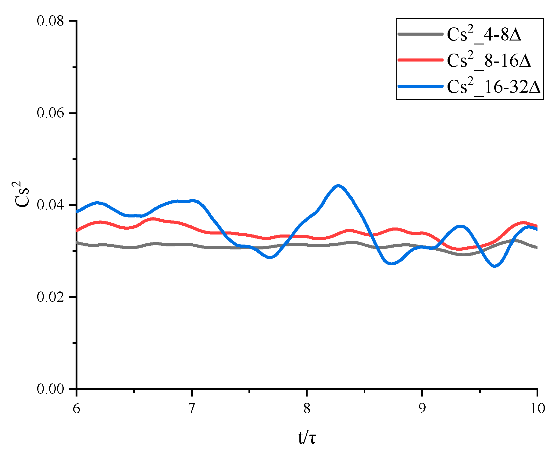
Figure 6.
The curves of the dynamic sub-grid temperature variance model coefficient
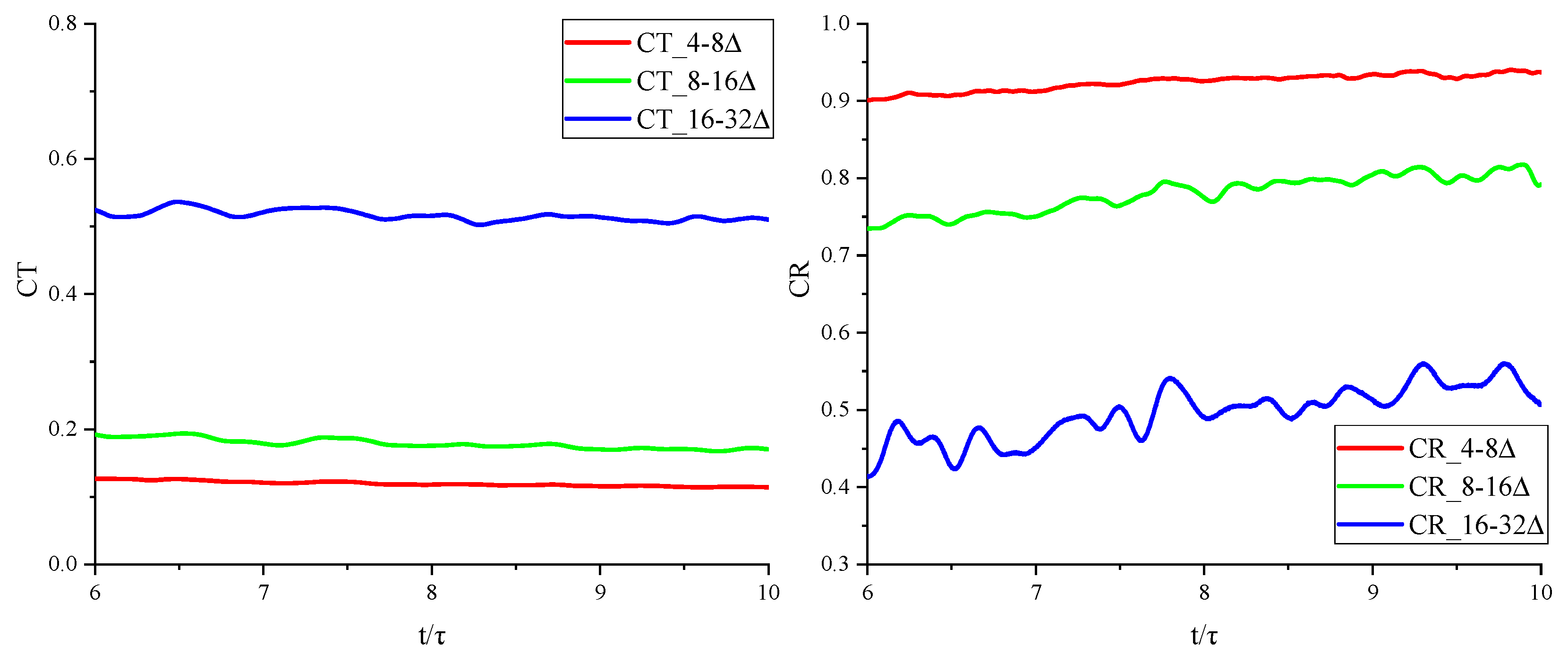
Figure 7.
The variation of the dimensionless sub-grid temperature variance (real values) and the calculated values from the dynamical temperature variance model over time at different filter scales.
Figure 7.
The variation of the dimensionless sub-grid temperature variance (real values) and the calculated values from the dynamical temperature variance model over time at different filter scales.
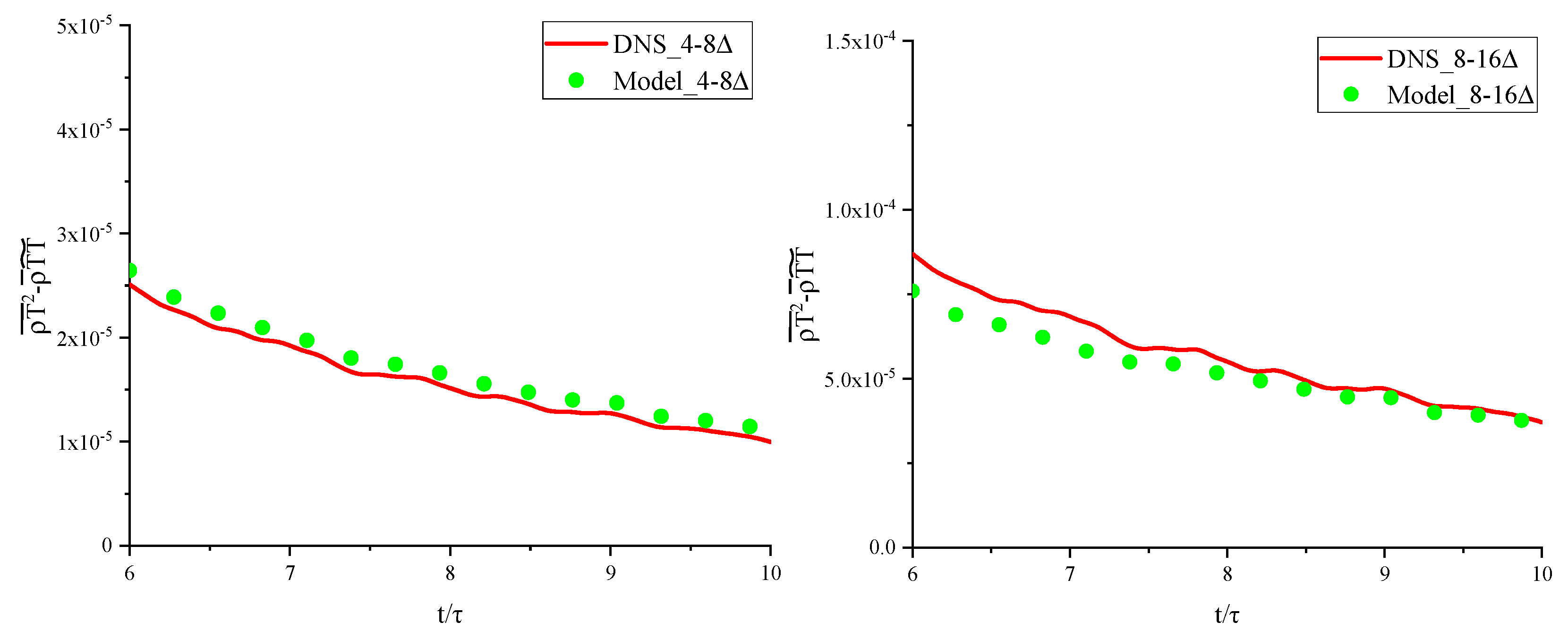
Figure 8.
When
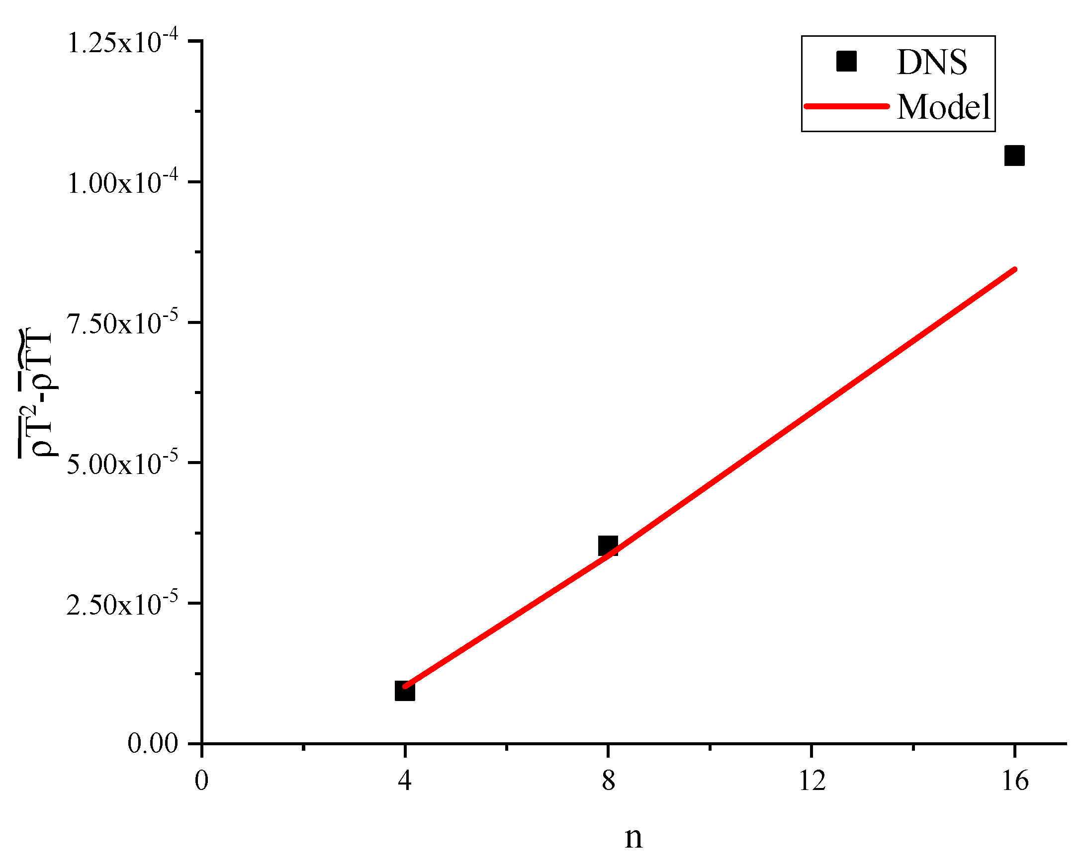
Figure 9.
Time evolution of gas components and temperature correlation coefficient in chemical-freezing isotropic turbulence flow field.
Figure 9.
Time evolution of gas components and temperature correlation coefficient in chemical-freezing isotropic turbulence flow field.
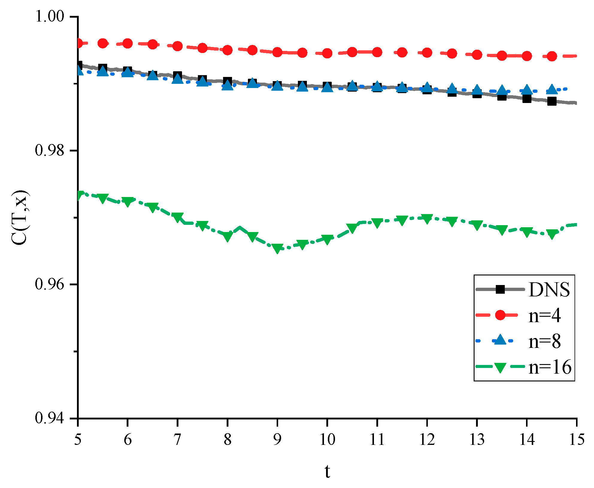
Figure 10.
Distribution of instantaneous Mach number and temperature at jet meridian plane.
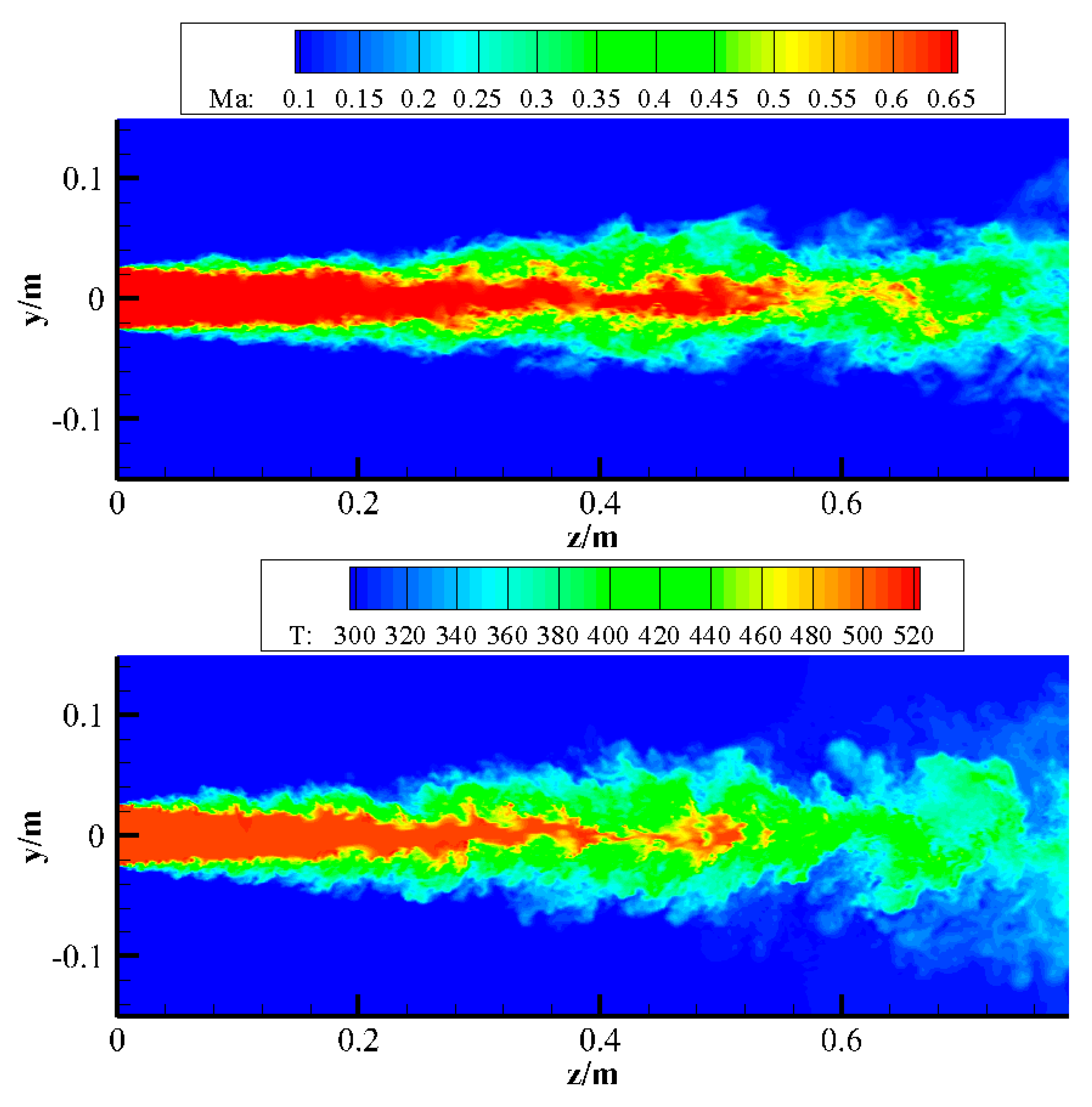
Figure 11.
Iso-surface of Q=107 colored with local temperature.
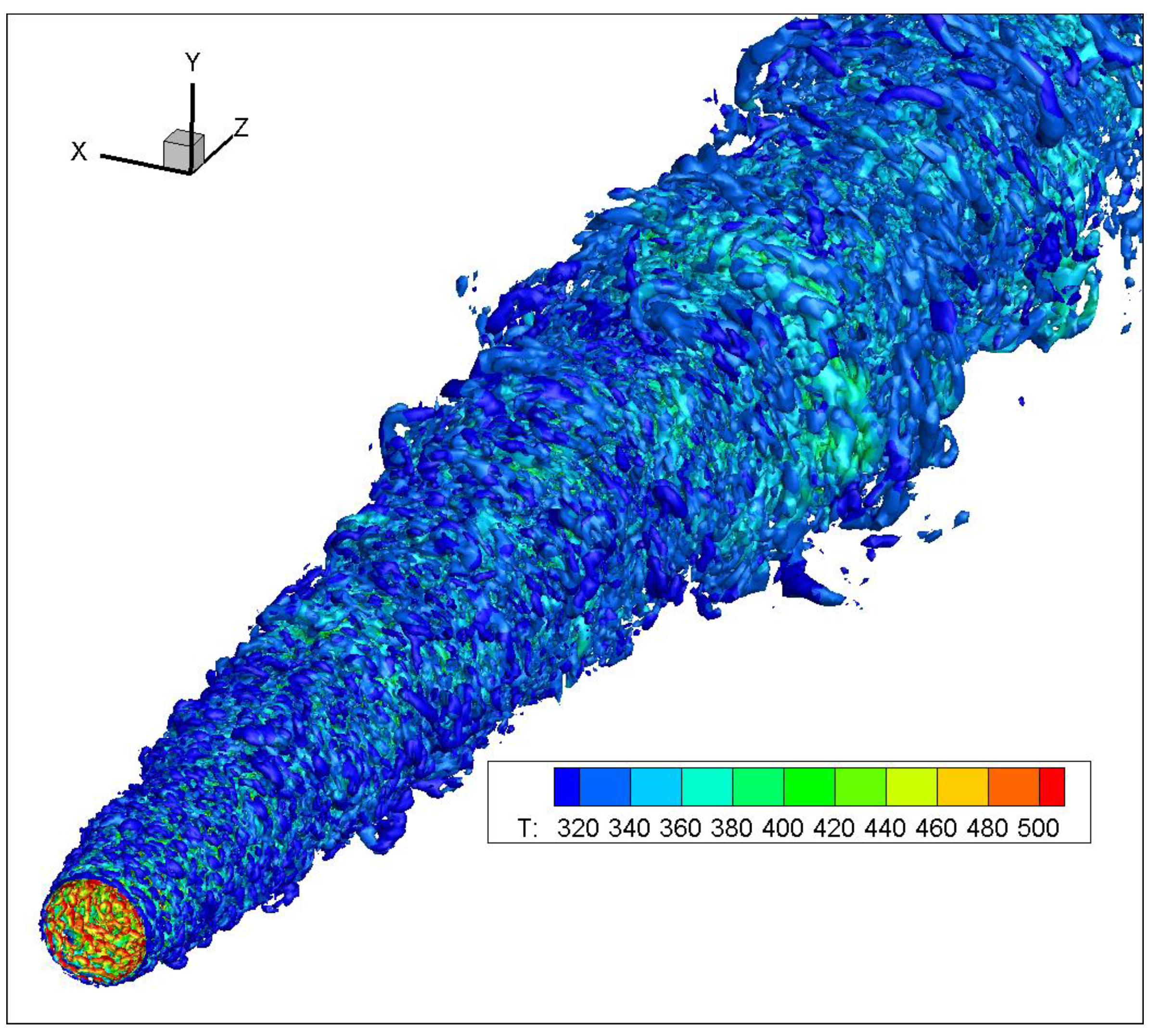
Figure 12.
Schematic diagram of nozzle and jet structure and the variation curve of various statistics along the flow direction at the center line and lip line.
Figure 12.
Schematic diagram of nozzle and jet structure and the variation curve of various statistics along the flow direction at the center line and lip line.
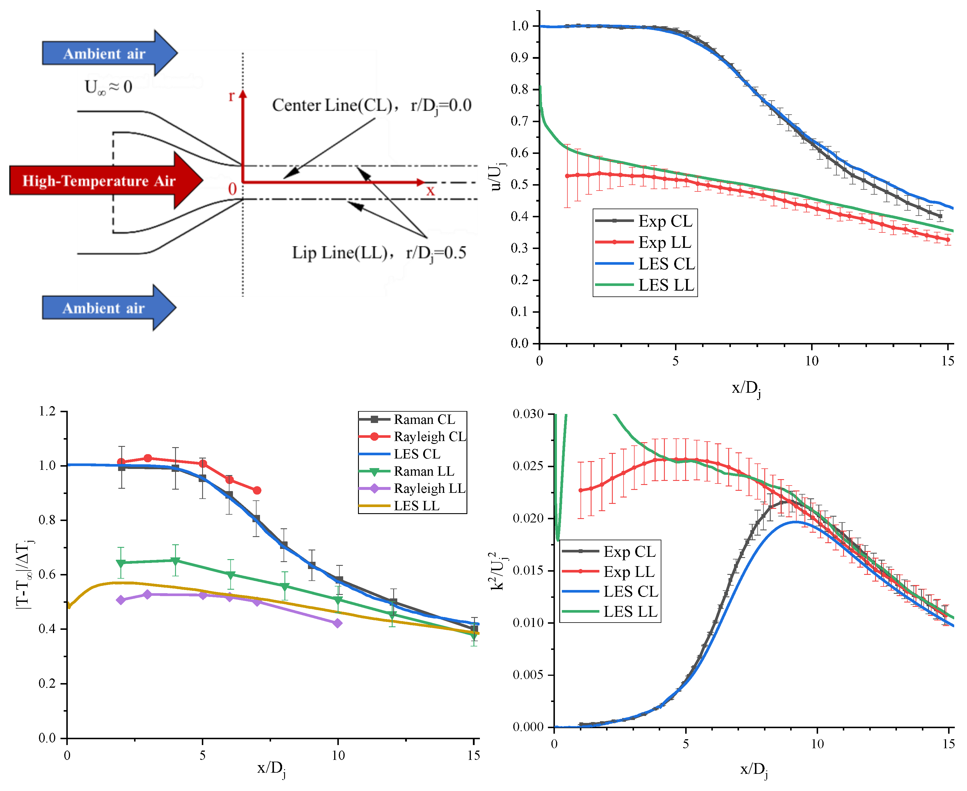
Figure 13.
Radial temperature profile at various flow field cross sections.
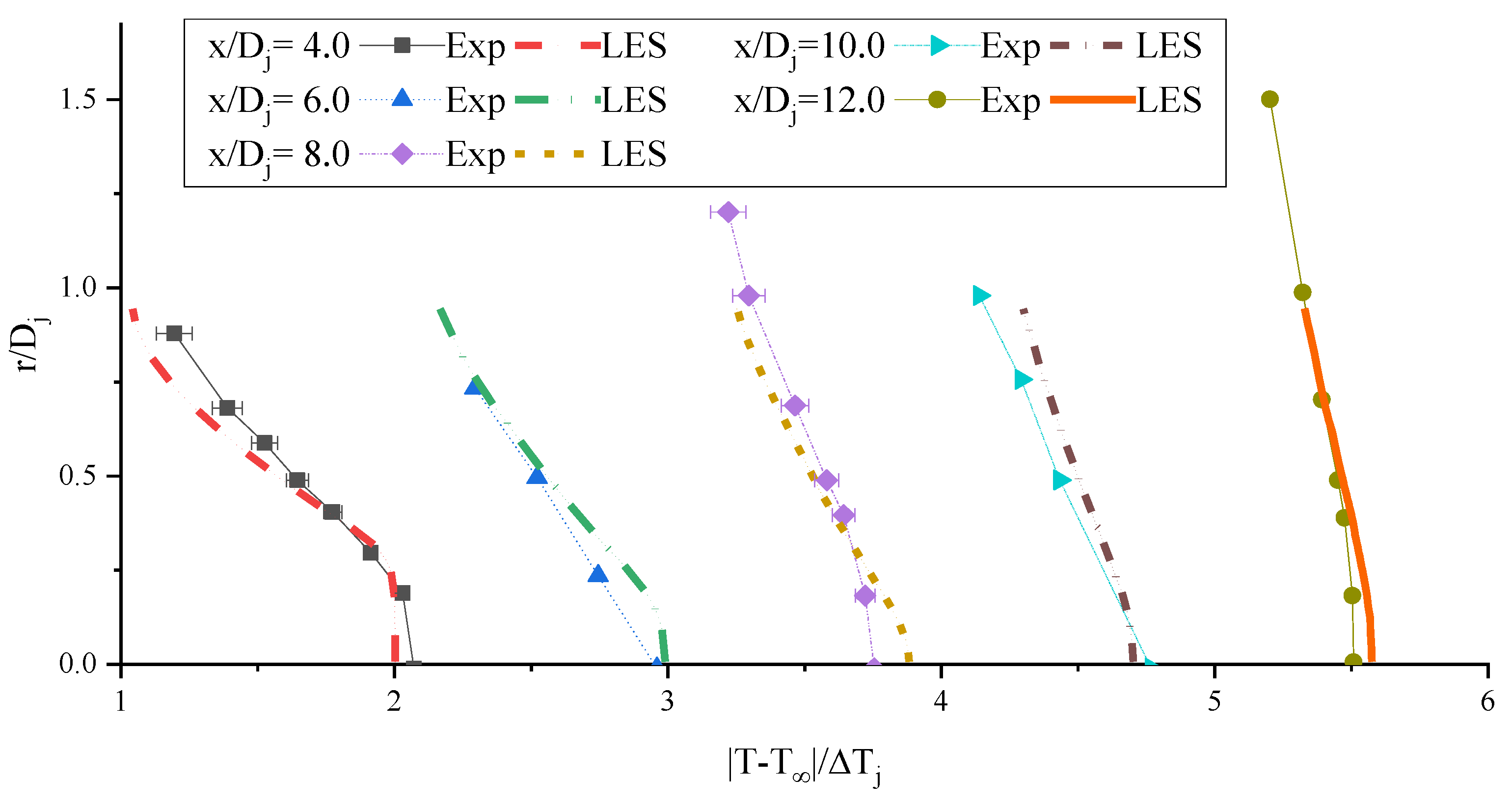
Figure 14.
Spectral extinction coefficients of aerosols involved in case 1 and 2.
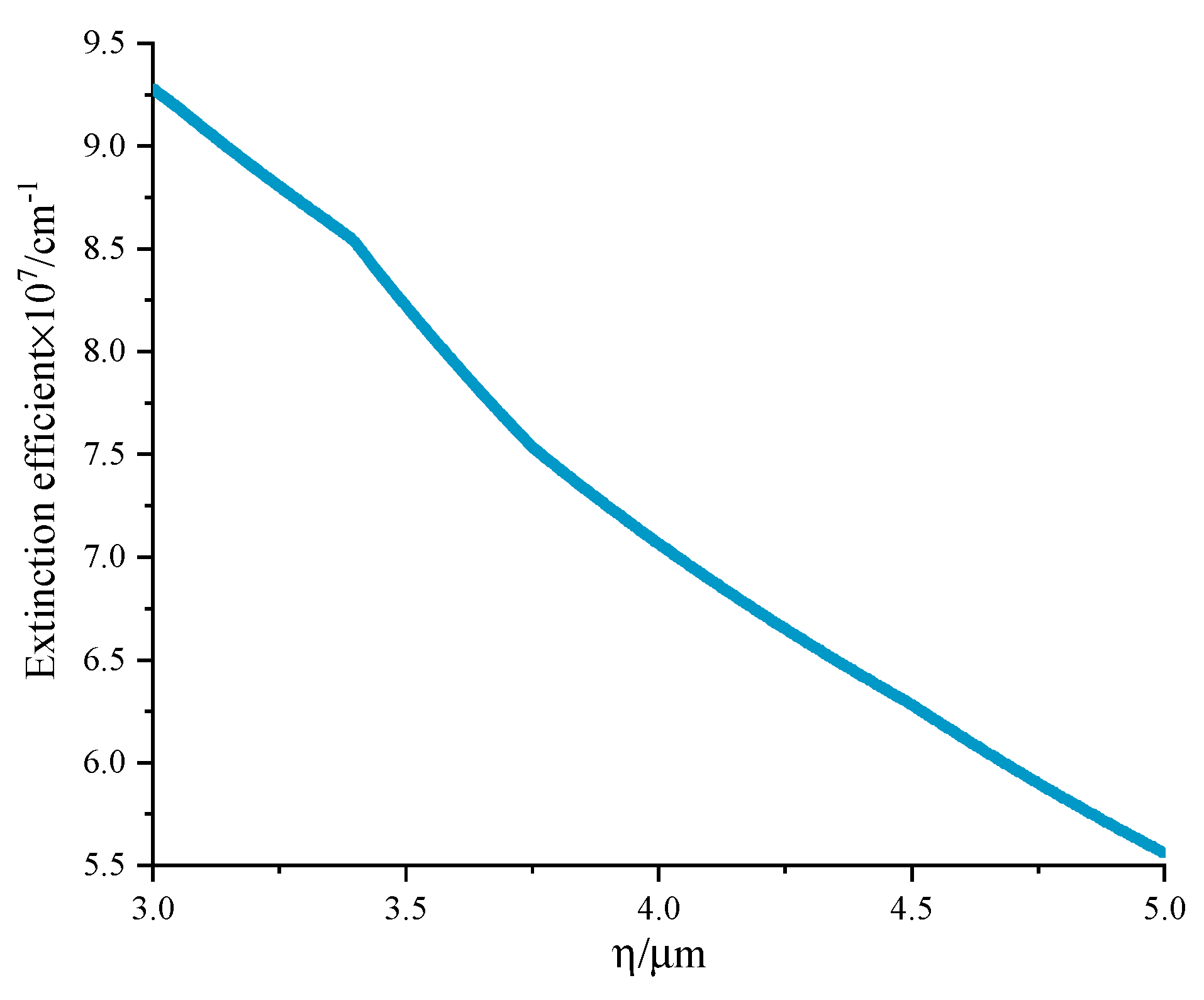
Figure 15.
Remote instantaneous infrared imaging and calculation error distribution of MSMGWB model in case 2(45km detection distance).
Figure 15.
Remote instantaneous infrared imaging and calculation error distribution of MSMGWB model in case 2(45km detection distance).
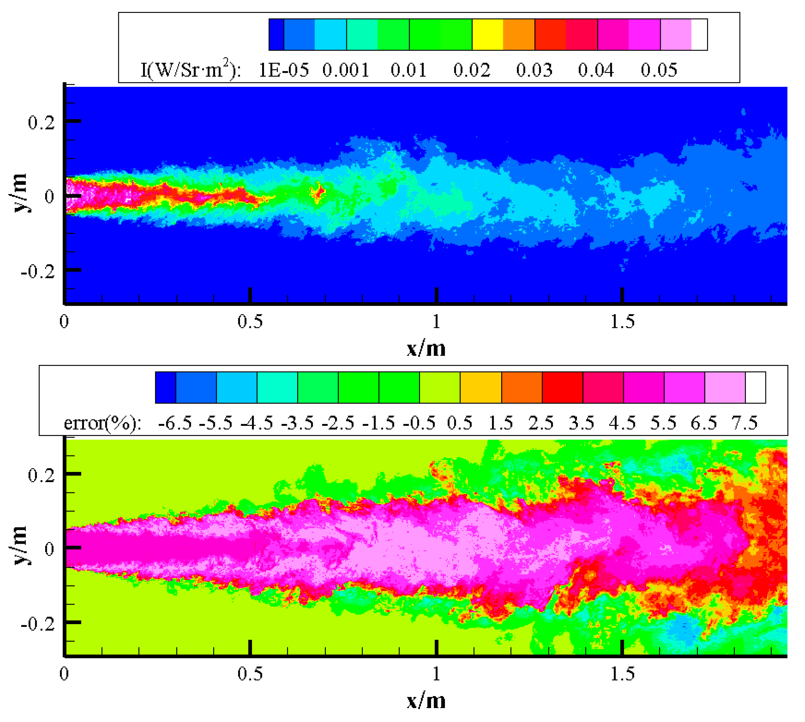
Figure 16.
Remote infrared images at 0.2km (upper)and 45km (lower) distances calculated based on average flow field of combustion gas jet.
Figure 16.
Remote infrared images at 0.2km (upper)and 45km (lower) distances calculated based on average flow field of combustion gas jet.
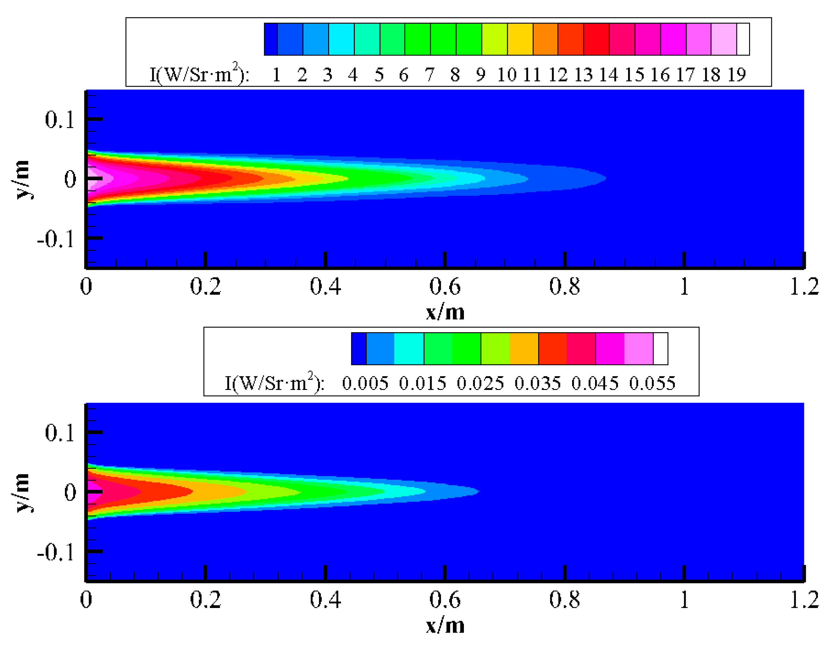
Figure 17.
Average remote infrared images at 0.2km (upper)and 45km (lower) distances calculated based on instantaneous flow field of combustion gas jet.
Figure 17.
Average remote infrared images at 0.2km (upper)and 45km (lower) distances calculated based on instantaneous flow field of combustion gas jet.
Figure 18.
Distribution of the percentage increase of jet flow infrared radiance attributed to TRI.
Figure 19.
Time evolution curves of normalized radiation intensity for various positions of combustion gas jet in case 1(up) and case2(down).
Figure 19.
Time evolution curves of normalized radiation intensity for various positions of combustion gas jet in case 1(up) and case2(down).
Figure 20.
Time evolution curves of normalized integrated radiation intensity for combustion gas jet in case 1(up) and case2(down).
Figure 20.
Time evolution curves of normalized integrated radiation intensity for combustion gas jet in case 1(up) and case2(down).
Figure 21.
Influences of TRI and SGS-TRI in case 1 at various detection distances.
Figure 22.
Influence of TRI and SGS-TRI in case 2 at various detection distances.
Figure 23.
Analysis of the characteristics of main contributing RTE’s for combustion gas infrared radiance at 45km (left) and 0.2km (right) detection distances.
Figure 23.
Analysis of the characteristics of main contributing RTE’s for combustion gas infrared radiance at 45km (left) and 0.2km (right) detection distances.
Disclaimer/Publisher’s Note: The statements, opinions and data contained in all publications are solely those of the individual author(s) and contributor(s) and not of MDPI and/or the editor(s). MDPI and/or the editor(s) disclaim responsibility for any injury to people or property resulting from any ideas, methods, instructions or products referred to in the content. |
© 2024 by the authors. Licensee MDPI, Basel, Switzerland. This article is an open access article distributed under the terms and conditions of the Creative Commons Attribution (CC BY) license (http://creativecommons.org/licenses/by/4.0/).
Copyright: This open access article is published under a Creative Commons CC BY 4.0 license, which permit the free download, distribution, and reuse, provided that the author and preprint are cited in any reuse.


