Submitted:
23 October 2024
Posted:
24 October 2024
You are already at the latest version
Abstract
The agriculture industry is critical to the global economy, with product quality having a direct impact on marketability and waste management. Apples, one of the most extensively produced fruits, are affected by a variety of diseases that can reduce productivity and quality. Accurate diagnosis of diseases is critical, but traditional manual approaches are time-consuming, error-prone, and ineffective. Inadequate labeled data and a wide range of disease symptoms make it necessary to design an automated, robust, and accurate system. This article describes a hybrid model for Apple Fruit Disease Detection (HMAFDD) that combines the strengths of three pre-trained convolutional neural network (CNN) models: ResNet50, DenseNet121, and EfficientNetB0. It accomplish this by using multi-architecture feature extraction. The hybrid system, which combines both models, is able to recognize a wide range of features, from simple textures to complex patterns unique to a certain diseases. Grad-CAM, or gradient-weighted class activation mapping, creates heatmaps that highlight significant regions for prediction, which enhances the interpretability of the model.To increase robustness and accuracy, techniques such as spectral-shifted adversarial perturbation for data augmentation and spectrally-weighted global average pooling for feature aggregation are used. This technique provides 99.75% accuracy with minimal processing needs, making it acceptable for real-time applications in agricultural situations. This considerably improves apple disease management.
Keywords:
Deep learning
; apple fruit disease
; convolutional neural network(CNN)
; Resnet50
; Densenet121
; EfficientnetB0
1. Introduction
Agriculture has an significant role in the global economy, by ensuring food security and encouraging economic stability [1]. A key factor in the success of agricultural industries is the quality evaluation of their products, which directly impacts marketability and waste management control [2]. Apples, one of the most widely consumed fruits globally, hold significant cultural, dietary, and economic importance. Alongside bananas, grapes, and oranges, apples rank among the top four most produced fruits worldwide. While apple production has increased over the last decade, this growth has not kept pace with the expansion of cultivation areas [3]. Apple farming is widespread, contributing significantly to the agricultural output of many countries. Ensuring that damaged apples are separated from healthy ones during post-harvest processing is crucial for maintaining high quality for consumers [4].
However, a lack of labeled training data and an extensive range of symptoms make it difficult to appropriately diagnose diseases in apples. Manual detection is a lot of work, takes a long time, and is prone to errors [5]. Advances in deep learning have transformed disease detection, allowing for the rapid diagnosis of complicated symptoms. These approaches have been applied across numerous fields, including fruit disease identification. Deep convolutional neural networks (DCNN) have provided outstanding results [6].
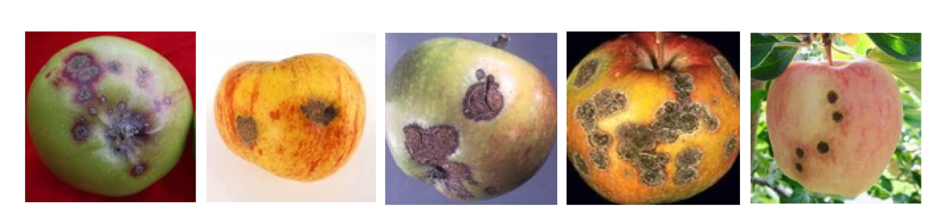
Automating disease detection using computer vision significantly improves the accuracy and speed of diagnosis, contributing to both economic growth and productivity [7]. Automation also enhances the fruit industry’s ability to maintain high-quality yields and reduce losses. In this paper, we present an HMAFDD that use Multi-Architecture Feature Extraction to categorize various apple diseases and highlight impacted regions. Gradient-weighted Class Activation Mapping (Grad-CAM) is a method used to emphasize the sick region on the fruit. Grad-CAM overlays a heatmap on an image to show the regions that influenced the model’s forecast the most. This interpretability features is critical in real-world applications because it allows users to quickly identify diseased areas, which leads to improved sorting, grading, and treatment decisions. Apple rot (deep tan to brown blotches), apple scab (corky brown scabs), and apple blotch (surface olive-green patches) are among the diseases discussed, along with healthy apples. Images of blotch apple, normal apple, rot apple, and scab apple are displayed in Figure 1, Figure 2, Figure 3 and Figure 4, respectively.
This hybrid technique improves accuracy in identifying apple diseases by combining the capabilities of ResNet50, DenseNet121, and EfficientNetB0, resulting in a robust solution for automated detection and classification.
1.1. Apple Diseases
A brief description of these disease is given here:
1.1.1. Blotch Apple:
Apple blotch is a damaging fungal disease that results in significant crop losses and is caused by Marssonina coronaria. The disease causes premature defoliation, black patches on apple fruits and leaves, dropped tree vigor, and reduced output. It also disrupts the host’s physiological balance [8]. If apple blotch is not treated, it can cause severe instances that eventually kill the tree. Cultural measures including trimming to improve air circulation, keeping trees spaced properly, and removing diseased leaves are advised in order to treat this disease. Fungicides can also be used as a prophylactic measure to guard against apple blotch. In apple orchards, early discovery and routine monitoring are essential to halting the development of this devastating fungal disease.
1.1.2. Scab Apple:
Venturia inaequalis is the fungus that causes apple scab. It damages crab apples and apples (Malus spp.), mountain ash (Sorbus spp.), pear (Pyrus communis), and Cotoneaster (Cotoneaster spp). A fungus that attacks both the leaves and the fruit is the cause of apple scab. Fruits with scabs are suitable for eating. Apple scab can be treated using fungicides. To effectively minimize disease, fungicides need to be applied at the appropriate period [9]. Planting resistant apple types can also minimize the likelihood of apple scab infection.
1.1.3. Rot Apple:
Apple rot is caused by the fungus Penicillium expansum and Monilinia fructigena. The fungus that causes fruit rots may be rather subtle, since spores will settle on the fruit and create symptoms after the fruit has been stored [10]. It is important to properly inspect fruit before storing it to prevent the spread of these fungi. Proper ventilation and storage conditions can also help reduce the risk of fruit rot.
Figure 1.
Blotch Apple Images
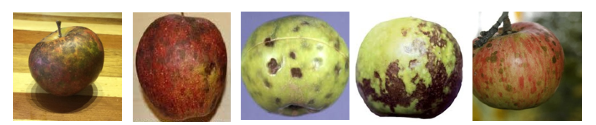
Figure 2.
Normal Apple Images
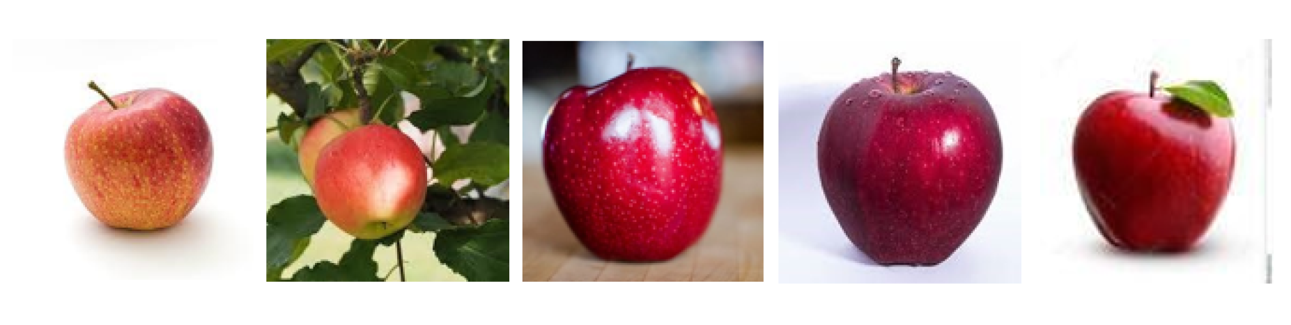
Figure 3.
Rot Apple Images
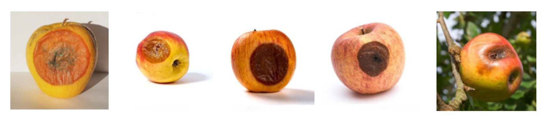
Figure 4.
Scab Apple Images
1.2. Challanges in Apple Disease Detection
Apple farming faces numerous challenges related to disease detection. Identifying apple diseases in real time is crucial for maintaining high yields and fruit quality. However, various factors, such as environmental conditions, varied disease symptoms, and limited labeled data, make disease detection a complex task. Traditional manual methods are labor-intensive, prone to human error, and not scalable. These methods often fail to distinguish between similar symptoms caused by different diseases, complicating the diagnosis. Using machine learning and deep learning to automate the detection process is an effective method to address these issues.
1.3. Advances in Deep Learning for Agriculture
Deep learning more specifically, convolutional neural networks, or CNNs—has transformed a number of industries recently, including agriculture. Convolutional Neural Networks (CNNs) have demonstrated considerable effectiveness in object identification, semantic segmentation, and image classification—all critical tasks for automating the diagnosis of diseases. In order to overcome the issue of low data availability, transfer learning using pre-trained models such as ResNet50, DenseNet121, and EfficientNetB0 has been used. Apple diseases categorization is made faster and more accurate with the help of these algorithms that extract hierarchical features from images.
1.4. Importance of Hybrid Models in Deep Learning
While single CNN models have shown great success, hybrid models that combine multiple pre-trained architectures offer enhanced performance. A hybrid model takes advantage of the capabilities of many architectures, capturing a diverse range of features, from simple textures to complex patterns. This results in a more robust and accurate model that can classify diseases with high precision. The hybrid model proposed in this study integrates ResNet50, DenseNet121, and EfficientNetB0, each contributing its unique strengths to improve disease classification accuracy.
1.5. Role of Explainability in Disease Detection
The interpretability of deep learning models is one of their primary issues in real-world applications. Grad-CAM is a tool for analyzing the model’s decision-making process. It highlights the regions of an image that the model uses to generate predictions. This is particularly important in agricultural settings, where actionable insights—such as the location and severity of a disease—are crucial. By generating heatmaps, Grad-CAM enables farmers and experts to understand why the model predicts a certain disease, ensuring trust in the system.
1.6. Applications of the (HMAFDD)
The proposed Hybrid Model for Apple Fruit Disease Detection has practical applications in various stages of apple farming and production. It can be integrated into real-time monitoring systems for orchards, where images of apples are continuously analyzed to detect early signs of disease. In post-harvest processing, the system can be used to automatically sort healthy apples from diseased ones, reducing the reliance on manual sorting and improving the overall quality control process. Moreover, the system’s interpretability feature makes it suitable for educational purposes, helping to train agricultural workers in identifying common apple diseases.
1.7. Significance of Study
The significance of this work stems from its ability to increase both scientific understanding and practical use of machine learning in agriculture.
1.7.1. Scientific Contribution
This study contributes to the expanding amount of research on using deep learning to agricultural difficulties. While single-model architectures have been widely studied, the integration of multiple architectures in a hybrid model is a relatively new approach. By establishing the positive impacts of this strategy, the study provides understanding of hybrid models’ ability to solve complex and variable challenges, such as crop disease detection. Future research on machine learning in agriculture may be influenced by the study’s findings, which might contribute to the development of more robust and effective models.
1.7.2. Practical Implications
There are important practical consequences to this work, especially for the apple industry. By providing a more precise and reliable technique for identifying and diagnosing apple diseases, the hybrid model has the potential to enhance disease management procedures in apple orchards. This, in turn, might reduce the need for chemical treatments since diseases can be recognized and handled more quickly and more efficiently.
1.7.3. Environmental and Economic Impact
Beyond immediate advantages to the apple industry, developing more precise disease detection systems has vast environmental and economic consequences. By minimizing the need for chemical treatments, the hybrid model may help to promote more sustainable agricultural techniques, minimizing the environmental effect of apple production. Furthermore, by enhancing disease management efficiency, the model has the potential to minimize crop losses, so contributing to food security and economic stability in regions where apple production is a major industry.
1.7.4. Summary:
The importance of this research extends beyond the technical creation of a new model. By addressing a critical problem in apple production, the research has the potential to contribute to more sustainable and profitable agriculture, with benefits for both farmers and consumers. The findings of this study may have greater consequences for the application of machine learning in agriculture, providing the way for the development of more advanced and practical models in in the future.
This research is structured in six sections. The previous research on this issue discusses in Section 2 . The problem description explains in Section 3. The contribution of work is then completed in Section 4. The provided approach is described in section . The experimental evaluation are discussed in Section 6. Finally, Conclusion and Future Work are discussed in section .
2. Related Work
Significant progress has been made in the identification and classification of plant diseases, especially in fruit crops like tomatoes and apples, due to the quick development of deep learning technology. Because Convolutional Neural Networks (CNNs) are better at extracting information from plant images, they have become a crucial component of many disease detection models. Remarkable architectures including ResNet, DenseNet, and EfficientNet have found widespread use due to their outstanding feature representation capabilities, especially in handling complex visual patterns like images of fruit or damaged leaves. Following description gives a concise overview of related work for system’s contributions to the field. Improtant information of Literature Review is presented in Table 1
In paper [11], the researchers established a new method for identifying fruit diseases using a hybrid model that includes a modified convolutional neural network (CNN) supplemented by a vision transformer. The collection includes images of six different fruits: apples, bananas, guavas, limes, oranges, and pomegranates. Further classified into healthy and diseased stages. During the pre-processing phase, the images undergo several transformations, including scaling, resizing, reshaping, and normalization of pixel values to a [0,1] range, followed by standardization. The CNN component of the model derives spatial feature extraction using convolutional layers triggered by ReLU functions, whereas the output layer uses a softmax activation function. Pooling layers within the CNN reduce the model’s spatial dimensions as well as its computational needs. Alternatively, model’s vision transformer feature analyze images by classifying them into uniform patches that include positional embeddings. These patch embeddings then go through a transformer encoder sequence. A head performs the final classification, which yields probabilities for each fruit condition that help in determining the most likely group based on the maximum likelihood.
In paper [12], author present an automated technique for detecting diseases in apple using Deep Spectral GAN(DSGAN) and DenseNet CNN. The initial preprocessing steps include the application of Median and Gabor filters, followed by edge delineation using Canny edge detection and segmentation through Self-Adaptive Plateau Histogram Equalization (SAPHE). The DSGAN framework is tailored to recognize apple diseases by analyzing variations in size and color through a structured network comprising input, hidden, and output layers. For the training and classification of apple diseases, a DenseNet Recursive CNN (DNRCNN) is employed. This model incorporates bilateral filtering, conversion to [HSV color space], and Canny edge detection in the preprocessing and segmentation phases. The feature extraction is enhanced by the neural chi algorithm and global mean pooling, while the DenseNet structure with recursive convolutional layers adeptly captures intricate patterns and features.
In paper [13], the authors provides a real-time detection method for apple leaf diseases based on deep learning techniques. The initial step involves image preprocessing, which encompasses resizing, normalizing, and augmenting the images. Several deep learning architectures, including convolutional neural networks (CNNs), densenet, generative adversarial networks (GANs), and transformer-based models, are used to automate feature extraction. Transformer models handle classification problems, whereas the DenseNet architecture is used for feature extraction. The cross-entropy loss function and the Adam optimization technique are used to train the DenseNet.
In paper [14], a approach for the identification and categorization of diseases affecting apples is proposed using image processing. The method starts with preprocessing the data and then uses K-Means clustering to segment the images. Features are extracted using the Gray Level Co-occurrence Matrix (GLCM), and they are then classified using the Naive Bayes method. With a classification accuracy of more than 96.43%, this method effectively detects and categorizes three prevalent apple diseases: apple blotch, apple rot, and apple scab.
In paper [15], a methodology for identifying and categorizing diseases in apples via convolutional neural networks is introduced. The first stage is preprocessing the image, which entails resizing it to 256x256 pixels and using a number of augmentation techniques, including cropping, flipping, scaling, and color adjustments. Five distinct architectures with various convolutional and fully linked layer configurations are examined in the study. All architectures has max pooing layers and uses ReLU activation functions. The Adam optimizer is used to train these models. First, a learning rate of 0.0003 is used, and then, over the period of 20 epochs, a 32-batch batch size square gradient decay of 0.99 is implemented.
In paper [16], to diagnose physiological anomalies in apples, a composite model is created by combining standard neural machine learning approaches with convolutional neural networks (CNNs). The utilized dataset comprises 1080 original Apple images and an additional 4320 images generated through augmentation. The model employs five established CNN architectures, including VGG19, to derive deep feature sets. These features are subsequently processed using five distinct machine learning classifiers. Out of all these combinations, the VGG19(fc6) features produce the greatest mean accuracy when combined with a Support Vector Machine (SVM) classifier.
In paper [17], a novel web-based decision support system named DSSApple is introduced for the diagnosis of post-harvest diseases in apples. This system utilizes a dual-stream hybrid diagnostic methodology that integrates both image-based and expert-driven approaches. The image-based stream enables users to identify diseases by selecting images that display various symptoms. Concurrently, the Expert-Based Stream collects insights from users through a series of symptom-related questions. The integration of Bayesian networks (BNs) processes this collected feedback, thereby enhancing the system’s diagnostic precision and dependability.
In paper [18], the authors employed the ResNet architecture to develop a system for identifying and classifying diseases in apple leaves. The first step in image preprocessing is to split the apple leaf images by highlighting the green parts and background, which will isolate the unhealthy patches. After converting these images into the Lab color space, segmentation is improved by applying thresholds to the L*, a*, and b* channels in order to successfully isolate the leaves from the background. During the feature extraction step, the grayscale co-occurrence matrix (GLCM) is employed to assess the disease spot’s color and texture properties. Ten statistical texture metrics are provided by this method: skewness, energy, homogeneity, mean, standard deviation, entropy, and contrast. Two separate classifiers are created for the training phase: a health-disease classifier that separates healthy leaves from diseased leaves, and a disease-disease classifier that differentiates between various diseases including cedar rust, apple grey spot, and black star disease. To address classification problems, a linear kernel support vector machine is employed.
In paper [19], the author proposes an upgraded version of the ResNet-50 model specifically developed for the identification and categorization of insect infestations and apple leaf diseases. This refined model incorporates a novel approach to boost the accuracy of detecting apple leaf afflictions by utilizing the Apple Leaf 9 dataset. This dataset provides an excellent basis for analyzing the model’s performance because it include a broad variety of images that represent typical apple leaf conditions. The inclusion of the Coordinate Attention (CA) module, which maximizes the extraction of spatial and channel information, is a relevant innovation in this model. By doing this, background distractions are reduced and the model is able to concentrate on important features of pests and diseases. Moreover, the use of the Weight-Adaptive Multi-Scale Feature Fusion (WAMFF) technique enhances the ability to identify subtle and diverse symptoms of disease on leaves by facilitating the adaptive combination of data from many scales. The model makes use of transfer learning approaches, first fine-tuning initial weights from a ResNet-50 model that was previously trained on the ImageNet dataset using images of apple leaf disease. The model’s durability and capacity for generalization are enhanced by the artificial expansion of the training data through the use of online data augmentation techniques. The enhanced ResNet-50 model outperforms several recent deep learning architectures including AlexNet, VGG16, DenseNet, MNASNet, and GoogLeNet, as well as traditional models, with a top-1 accuracy rate of 98.32%. This demonstration highlights its exceptional efficacy in accurately identifying insect pests and diseases of apple leaves.
In paper [20], the author developes a multi-disease classification system for plants based on the DenseNet-121 architecture. This system is divided into various phases: images capturing, preprocessing, segmention, features extraction, and classification. The design seek to extract as much valuable information as possible from plant leaf images while remaining simple. The methodology makes use of 35,779 images from the Plant Village collection, which covers 29 different plant diseases in seven different plant species: potato, tomato, maize, bell pepper, grape, apple, and cherry. Every image is resized to 256 by 256 pixels. Images are first transformed from RGB to HSV color space. A binary mask is generated using a histogram-based threshold that concentrates on the H-channel data. This mask is applied to the source images to remove background and highlight disease-affected regions. The images are then downscaled to 64x64 pixels to reduce the computational load during training. The DenseNet-121 model, noted for its densely connected layers that allow for effective deep feature learning with low parameter counts, is utilized for feature extraction. These features are then sent into a classification layer, which assigns a disease category to each leaf image. With a learning rate of 0.002, the model is trained for 50 epochs using about 75% of the images for training and 25% for validation. In real-time evaluation, the model’s practical accuracy is 94.96%, while its theoretical accuracy on training data is 98.23%. Additionally, a web-based application that enables users to upload photos of plant leaves and receive a prompt diagnosis demonstrates the effectiveness of the technology.This application showcases the usefulness of the model in realistic situations.
In paper [21], by using deep learning techniques, researchers developed an artificial intelligence framework for identifying diseases in the leaves of apples, grapes, and citrus fruits. The original and corrected noisy datasets were the two sections of the dataset. Images of leaves from three different fruit varieties, divided into categories representing damaged and healthy leaves, made up the first dataset. To create the noisy dataset, various noise patterns, such as Gaussian and Rayleigh, were superimposed on the original images. The authors employed a fine-tuned Efficient-Net-B0 model to extract features from these images. They trained this model separately on the original and noisy datasets, resulting in two distinct models (Model 1 and Model 2). The extracted features from both models were then merged using a unique serial concatenation probability method to form a more distinct feature vector. To refine the feature selection, the Path Finder Algorithm (PF), an enhanced meta-heuristic optimization technique, was utilized. This technique aimed to improve classification accuracy by identifying most significant features and removing redundant data. A variety of machine learning classifiers, including Wide Neural Network, Medium Neural Network, and Support Vector Machine, were employed to classify the most effective feature vector that was generated. For every fruit dataset, the framework produced high classification accuracies: 100% for apples, 99.7% for grapes, and 93.4% for citrus fruit leaves.
In paper [22], the author describe a DCNN based approach for detecting diseases in apple leaves. Apple tree leaves are classified into four categories using images by a combination of pretrained DenseNet121, EfficientNetB7, and EfficientNet NoisyStudent: healthy apple, scab apple, cedar rot apple, and various diseases. The model can recognize leaves with many diseases with 90% accuracy.
In paper [23], an LSTM network and CNN models that pretrained are combined to create a hybrid model that is used to identify pests and diseases in apples. DenseNet121, AlexNet, and GoogleNet are used for feature extraction. The LSTM layer receives the extracted deep characteristics, which are then incorporated to creating a effective hybrid model that capable of detecting pests and apple disease. The tests employ real-time images from Turkey of pests and apple disease, and performance is evaluated by calculating the accuracy rates.
In paper [24], A review paper on Plant Disease Detection and Classification using Deep Learning was proposed by the author. The scientific advancement in deep learning methods for agricultural leaf disease detection is summarized. In this study, the author uses deep learning and sophisticated imaging techniques to examine current trends and difficulties in plant leaf disease identification.
In paper [25], an author suggested using nonlinear deep features as the basis for a classifier for Apple Disease. This paper explores many Deep CNN (DCNN) apple disease classification applications that leverage deep produced images for improved accuracy. To achieve this, the study progressively updates a baseline model using an end-to-end trained DCNN model, which has fewer parameters and higher recognition accuracy than prior models.
In paper [26], an author introduced a new 14-layer deep convolutional neural network (14 DCNN) for identifying plant leaf diseases using leaf images. This model is trained over 1000 epochs in an multi-graphical processing unit (MGPU) environment. Weighted average precision (99.7999%), weighted average recall (99.7966%), weighted average F1 score (99.7968%), and overall classification accuracy (99.9655%) were all attained with the DCNN model.
In paper [27], an author presented an effective and precise model for identifying diseases in plant leaves using the EfficientNet architecture. The technique comprises of multiple phases, including image capture, preprocessing, feature extraction, and classification. Initially corn leaf images are extracted from databases such as PlantVillage and PlantDoc. The preprocessing stage consists of converting the images to grayscale, performing Otsu thresholding for segmentation, and refining the discovered areas with morphological procedures. The GLCM (Gray-Level Co-Occurrence Matrix) approach extracts texture features such as contrast, correlation, and entropy. The EfficientNet design is used to do classification, maximizing the depth, width, and resolution for high accuracy while minimizing processing costs. The system is fine-tuned using pre-trained weights and tested on a variety of evaluation measures, including accuracy, sensitivity, and specificity, with an average accuracy for classification of 98.85%.
In paper [28], an author presented a system that can detect and analyzed fruits using image pre-processing with perfect accuracy. This suggested technique is consisted of the following basic steps: acquiring the input picture, image pre-processing, identifying impacted areas, and highlighting those affected spots. Verifying training set and displaying results. This technique employed photos of a few forms of fruit diseases, including bitter rot, sooty blotch, powdery mildew, and fungus. This strategy was studied in terms of fruit disease kind and stage, such as fresh and afflicted.
In paper [29], An author presented "AFD-Net: Apple Foliar Disease Multi-classification using Deep Learning on Plant Pathology Dataset," emphasizing the critical need for early and precise detection of plant diseases, particularly in apple crops, since they considerably affect agricultural productivity and quality. The system is structured to overcome limitations in current approaches, such as sensitivity to image variations and imbalance in disease categories. AFD-Net uses EfficientNet-B3 and EfficientNet-B4 as backbone topologies, which are noted for their scalability and efficient parameter consumption. The suggested AFD-Net model outperformed existing deep learning models in the original and expanded datasets, achieving 98.7% accuracy for Plant Pathology 2020 and 92.6% for Plant Pathology 2021.

Table 1.
Literature Review.
| Author | Technique | Advantages | Problem Identified |
|---|---|---|---|
| Smit Zala, Vinat Goyal,Sanjeev Sharma, andAnupam Shukla [11] | Customized CNN and Vision Transformer | Emphasize the effectiveness of deep learning, particularly Vision Transformer, in accurately and reliably classifying fruits | Monitoring fruit diseases manually is time-intensive and requires expertise, which is often lacking in remote regions. |
| V. Subha and K. Kasturi [12] | Deep Spectral GAN and DenseNet CNN | An optimized classification approach that boosts accuracy and specificity in real-time applications. | Poor segmentation and low sensitivity in current studies hinder better apple disease classification. |
| Asif Iqbal Khan, S.M.K. Quadri, Saba Banday, and Junaid Latief Shah [13] | CNN, DenseNet, and Transformer | Rapid detection of apple leaf diseases can improve early intervention and help prevent agricultural losses. | Real-time apple leaf disease detection struggles with accuracy and efficiency due to diverse environmental conditions. |
| Sumanto, Yuni Sugiarti, Adi Supriyatna, Irmawati Carolina, Ruhul Amin, and Ahmad Yani [14] | GLCM and Naïve Bayes | Combining GLCM feature extraction with Naive Bayes created a highly accurate system for detecting and classifying apple diseases. | A limited image collection may limit the model’s usefulness in a variety of real-world circumstances. |
| Asmaa Ghazi Alharbi, Muhammad Arif [15] | CNN | To deliver high-quality products, it’s essential to separate damaged items, with automatic detection methods proving more effective than manual ones despite their limitations. | Detecting apple rot has lower classification performance than other diseases, underscoring the need for improved model accuracy. |
| Birkan Buyukarikan and Erkan Ulker [16] | VGG19(fc6) and Support Vector Machine (SVM) | Utilizes deep features extracted from images under varying lighting conditions, enhancing the reliability of early detection | Variability in classification accuracy caused by changes in lighting conditions during image acquisition, which affects the reliability of detecting physiological disorders in apples |
| Gabriele Sottocornolaa, Sanja Baric, Maximilian Nocker, Fabio Stella, and Markus Zanke [17] | Dual-stream hybrid approach: Image-based stream, Expert-based stream, and Bayesian Networks | Combining image-based and expert-based approaches improves diagnostic accuracy and user accessibility for detecting post-harvest apple diseases | Challenge of integrating diverse user inputs and symptom variations into a cohesive diagnostic framework, which may complicate the accuracy and reliability of the system’s recommendations |
3. Problem Definition
In the agricultural sector, the health of fruit crops is crucial for both maximizing production and ensuring the quality of the product because it is distributed globally. Apple orchards are particularly prone to a various kinds of diseases which can result in significant financial losses if not detected immediately and precisely. Historically, detecting these diseases has relied mainly on manual testing, which are not only time-consuming but also subjective and error-prone, frequently resulting in delayed answers. The main challenge is to create an automated, reliable, and precise system for detecting diseases that operates effectively in varied real-world farming conditions. Such conditions can introduce disturbances and distortions in the data, which complicates the detection and classification tasks. The system not only need to detect the presence of diseases but also accurately distinguish between different diseases affecting various fruit types, ensuring proper management for each specific condition. To overcome these problems, we present a hybrid model that uses pre-trained deep learning architectures—ResNet50, DenseNet121, and EfficientNetB0—to diagnose apple diseases and highlight areas of disease on the fruit. Our model integrates the strengths of these three powerful CNN architectures to improve accuracy in disease detection while minimizing computational complexity. By combining these models, our hybrid approach is designed to capture different levels of abstraction and detail from apple images, making it highly effective at distinguishing between healthy and diseased apples. This multi-architecture model can handle the complexity of various symptoms, such as the scabby lesions of apple scab, the olive-green patches of apple blotch, and the deep brown spots of apple rot.
4. Contribution of the Paper
Some objectives of our work are given below:
4.1. Increase Dataset
To generate more images from existing images Spectral-Shifted Adversarial Perturbation(SSAP) data augmentation method is utilized. The aim of SSAP is to create synthetic variats of the original images by combining small spectral shifts and adversarial perturbations to inprove the robustness and generalization capabilities of our apple disease detection system. This method strengthens the model’s resistance to adversarial attacks and variances in real-world scenarios while also increasing the size of the training data set.
4.2. Hybridization
Creating Hybrid model using pre-trained model (ResNet50, DenseNet121 and EfficientNetB0) and applying certain changes to these model, along with targeted changes, offers a substancial increase in apple disease detection. By integrating the various feature extraction strengths of ResNet50, DenseNet121, and EfficientNetB0, the hybrid model captures a wide variety of features that are crucial for accurately identifying apple diseases accurately. New hybrid mode (HRDE) equation is created [18] for our model. To minimize overfitting and loss, aggregation and regularization method employed.
4.3. Model Evaluation
By Our proposed Model, Model gives Best Accuracy on both training and Testing Data. By Limitation of Literature Review, Our model will Classified the Apple disease and Also Highlight the Particular Area of Disease if it has. and Also Evaluate the model performance we will add So many Graph such as Accuracy and Loss and Comparison with Positive Matrix, Comparison with Negative Matrix, Comparison with Other Matrix and Also Add Generalization of our model and So many more. These all Metrix and Graph and Results of our propose system Shows that our model Will be Best.
5. Materials and Methods
This proposed model is designed to detect diseases in apples by analyzing images of the fruit. The process starts with preparing the image. The image preprocessing guarantees that the input image is in the most suitable format for the model to interpret. Initially, the input image is read using an suitable image processing library. Once the image is loaded, it is resized to a fixed dimension of 224x224 pixels because pre-trained models like ResNet50, DenseNet121, and EfficientNetB0 expect input images of this size. After that, the image’s pixel values are normalized to the interval [0, 1]. In order to accomplish this, divide its total value of all pixels in an 8-bit image by 255, the highest possible value that may be assigned to a pixel. After normalization, the dimensions of the image are expanded to include a batch dimension because the model expects a batch of images as input. The expansion is typically done by adding an extra dimension to the image array, transforming it from a shape of (224, 224, 3) to (1, 224, 224, 3). This expanded dimension represents the batch size, which is 1 in this case. After expansion, the data augmentation technique is applied to the expanded image to make a more robust model.
Next, the preprocessed input image undergoes a series of transformations through multiple pre-trained CNNs (ResNet50, DenseNet121, and EfficientNetB0) to extract meaningful features. Initially, the top layers of these models, typically responsible for classification, are removed to repurpose the networks solely as feature extractors. The pre-processed image, resized to 224x224 pixels and normalized, is then fed into each of these models. As the image traverses through the convolutional layers of ResNet50, DenseNet121, and EfficientNetB0, hierarchical features are retrieved at different levels of abstraction. These features capture important patterns including edges, textures, and more complicated structures that might help to diagnose apple diseases. The output from each model is a high-dimensional tensor representing the extracted features.
Next, in the feature aggregation step, the goal is to combine the rich feature representations extracted from multiple pre-trained models to form a comprehensive feature vector that encapsulates the essential characteristics of the input image. It is passed through three different pre-trained models: ResNet50, DenseNet121, and EfficientNetB0. Each of these models has been trained on a large dataset and can recognize different levels of abstraction in the image data. To employ these models as feature extractors, the top layers, which are usually responsible for categorization, are eliminated. This allows us to access the intermediate layers that contain the learned features. As the image passes through each model, a high-dimensional feature map is produced. To minimize dimension and focus on the most relevant features, each feature map is subjected to global average pooling. This approach averages all of the values in each feature map, producing a fixed-size vector for each model, independent of the feature maps’s original dimensions. These pooled feature vectors from ResNet50, DenseNet121, and EfficientNetB0 are then concatenated into a single, unified feature vector. This concatenation effectively combines each model’s unique viewpoints and capabilities, resulting in a strong and complete representation of the input image. The input for the model’s succeeding layers is this aggregated feature vector, which guarantees that the classification decision based on a variety of features. The regularization metyhod minimizes overfitting and makes sure that the model generalizes effeciently to fresh data. Regularization is implemented using a dropout layer, which works by randomly changing a fraction of the input units to zero throughout the training phase, breaking up co-adaptations between neurons and forcing each neuron to learn to work independently and contribute to the final prediction rather than relying on other neurons. The model acquires stronger features from this randomization, which reduces the likelihood of the training dataset being overfit.
Next, we train the hybrid model (ResNet50, DenseNet121, and EfficientNetB0). For multiclass classification, we first employ the Adam optimizer with a learning rate of 0.0001 and the categorical cross-entropy loss function. To prevent the overfitting and improve training efficiency, we utilize two callbacks: EarlyStopping and ReducedROPlateau. EarlyStopping determines validation loss and stops training if it does not improve after 10 consecutive epochs, restoring the best weights seen throughout training. With a learning rate threshold of 0.00001, ReduceLROnPlateau also tracks the validation loss and lowers the learning rate by 0.2 if no improvement is observed after 5 epochs. The training data generator is then used to train the model for a maximum of 50 epochs, and a different validation data generator is used to validate the results. The model is trained by continuously running batches of images through it, calculating the loss, and then adjusting the model weights to minimize this loss. The callbacks provide the best possible training dynamics and model generalization. The dense layer is then fitted with a softmax activation function, which is required for multi-class classification tasks, and the diseased region is highlighted in the image using a Grad-CAM method. The softmax function transforms the dense layer’s raw output scores (logits) into a probability distribution across all possible classes. The probability distribution indicates the likelihood that an image belongs to a specific class. Grad-CAM provides a heatmap overlay on the images, visually indicating the areas that contributed the most to the model prediction. Grad-CAM technique initially converts the image to grayscale to simplify the image data and make it easier to perform further processing. The grayscale image was then separated into diseased (foreground) and healthy (background) parts using a binary threshold. An image can be converted to a binary image with pixel values of 0 (black) or 255 (white) using binary threshold. Next, contours are identified by analyzing the binary image. Curves known as contours connect every continuous point along a border with its corresponding color or intensity. These contours aid in highlighting the areas of the original picture that are diseased. Next, draw the identified contour onto the original RGB picture. This highlights the diseased parts, making them easily distinct from the healthy portions. Finally, the original image is displayed alongside the predicted disease class, with an emphasis on visualizing the affected areas. If the model identifies the apple fruit as diseased, the image is presented with an overlay highlighting the regions deemed potentially diseased. Conversely, if no disease is detected, the image is shown with a message indicating the absence of diseased areas. This visualization is crucial for interpreting the model’s predictions, enabling researchers and practitioners to pinpoint exactly where the model has identified disease on the apple fruit, thereby providing a visual confirmation of the detection process.
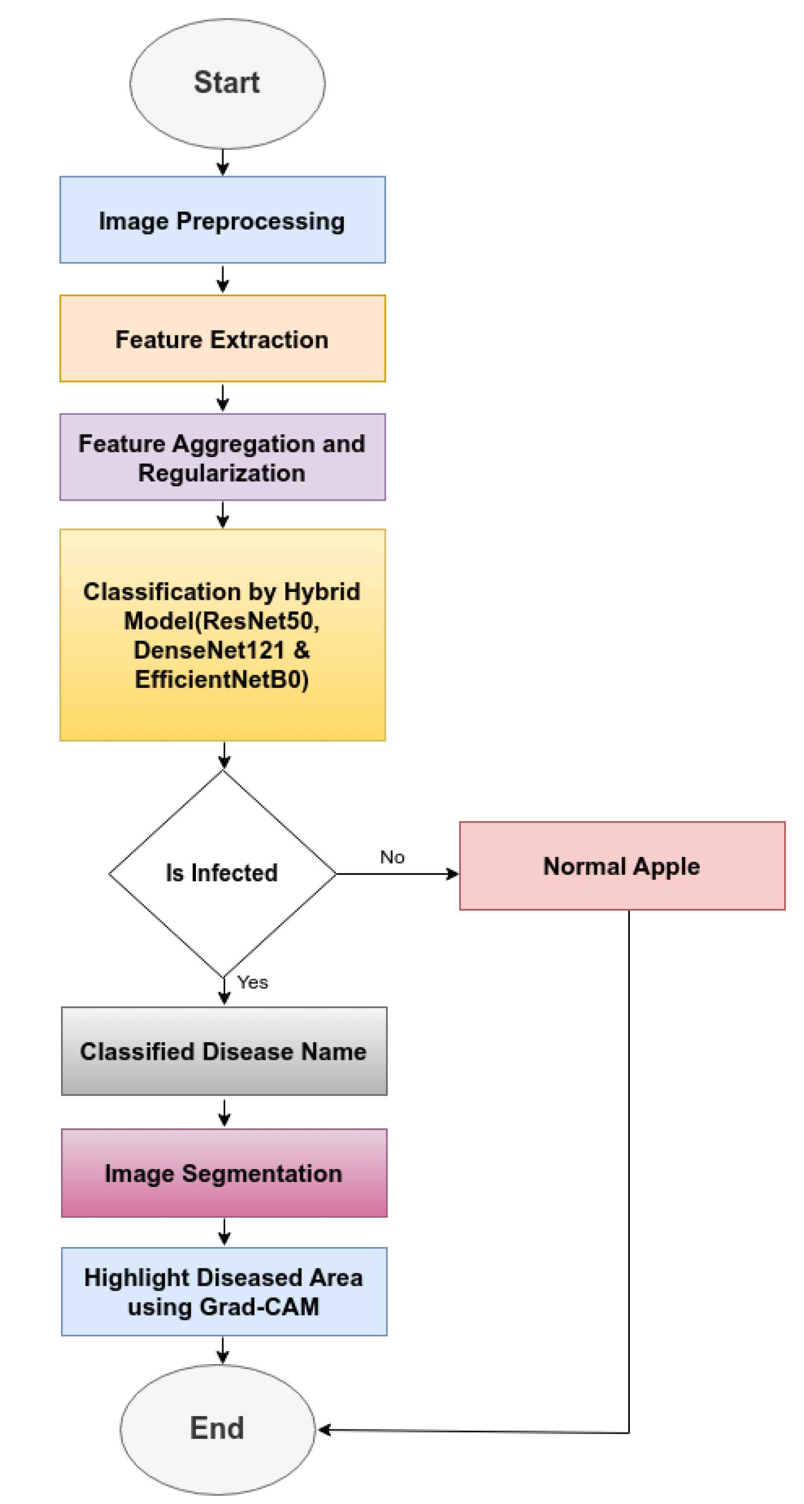
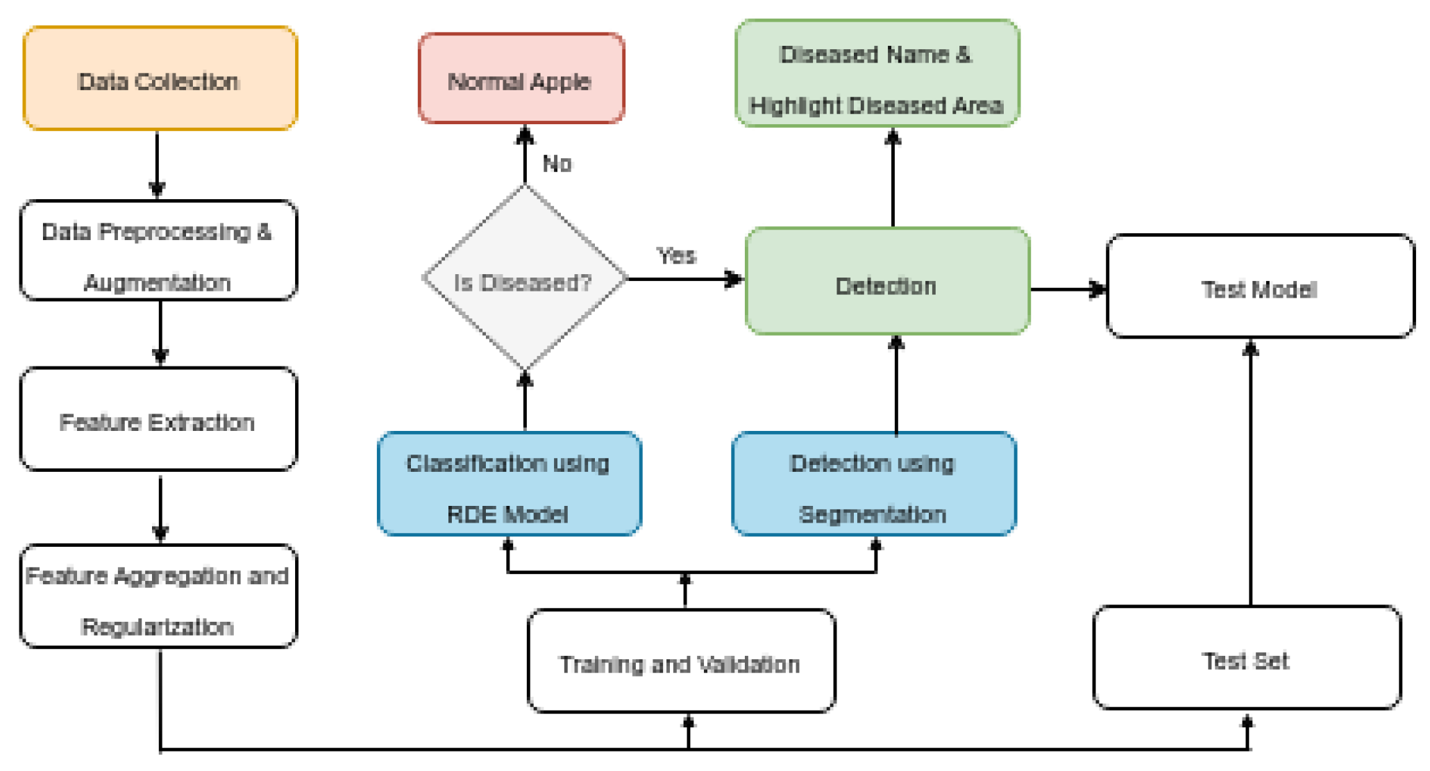
The modelling of hybrid model for apple fruit diease detection (HMAFDD) is shown in Figure 5. We first gathered the dataset and then improved its quality using preprocessing and augmentation approaches. For dataset classification, hybrid models of ResNet50, DenseNet121, and EfficientNetB0 were created and trained using a variety of hyperparameters. All hyperparameters are included 541 in the Table 5. Then categorize and highlight the affected region of the apple disease picture. The flowchart and architecture of HMAFDD is shown in Figure 6 and Figure 7
5.0.0.1. Phases of Proposed System
- Phase-1: Apply pre-processing on the input image, including resizing, normalization, and expanding dimensions to include the batch size.
- Phase-2: Extract features using pre-trained models (ResNet50, DenseNet121, EfficientNetB0). Apply global average pooling to reduce feature maps and concatenate the pooled vectors into a single feature vector. Combine feature vectors from all three models into unified vectors.
- Phase-3: Apply dropout to prevent overfitting.
- Phase-4: Pass aggregated feature vectors through a dense layer with softmax activation and compute class probabilities for the input image.
- Phase-5: Find the index of the highest probability and map it to the corresponding class name and highlight the diseased area using Grad-CAM.
5.1. Data Acquisition (Collection)
Data collection is a systematic process for obtaining relevant information in order to create a coherent and comprehensive dataset focused to certain business objectives, such as decision-making, research questions, or strategic planning. It denotes a beginning and crucial phase of data-driven operations and initiatives. The image data set used for identification was obtained from Kaggle and is publicly available as MADCB-DS (Modified Apple Disease with Class Balance-Dataset). The present paper picked the image of an apple fruit from the data set for analysis. Apple fruit collection includes pictures of blotch, healthy, rot, and scab apples as well as their symptoms. Images of all the diseases are displayed in Figure 1, Figure 2, Figure 3, and Figure 4. To facilitate identification, every symptom image was scaled to . The data collection comprises 5566 photos after the data augmentation procedure. The train and test subsets of the dataset are then separated into four categories: blotch apple, normal apple, rot apple, and scab apple. Based on the category label ratio within the dataset, randomly picked images were used to divide the produced dataset into training and test datasets in an 8:2 ratio. Of the symptom images, 80% were included in the training dataset for training and 20% for validation. To balance the classes within each subset, the undersampling approach is applied.
5.2. Data Preprocessing
Data has to be processed after it is gathered and then added to the model architecture. In data preparation, resizing the fruit image is essential as various model designs need for various input [30]. This stage involves downsizing, normalizing, and supplementing the size of the images provided to meet the model’s input parameters. This preprocessing step ensures that the input image is optimally formatted for efficient model processing.
Sub-Section 5.2.1 - Section 5.2.5 discussed the operations performed in Data Preprocessing
5.2.1. Resizing
Images in the dataset may be of varying dimensions, but machine learning algorithms normally require a fixed input size to ensure consistency. Consistent image dimensions enable the model to handle images effectively and without shape-related mistakes. This resizing aligns with the architecture of several pre-trained networks, such as ResNet, DenseNet, and EfficientNetB0, which are frequently trained on images of 224x224 pixels. Here, we utilize ImageDataGenerator for resizing. When an image is loaded, the target_size=(img_height, img_width) parameter in flow_from_directory() resizes it to the specified height (224 pixels) and width (224 pixels). This is critical for ensuring that the input to the neural network is uniform in size.
Each original image is resized to in equation [1
Where, is the Original Image. represent a function applying resizing technique to image. is the resulting Resized Image.
5.2.2. Normalization
To normalize standard range for images’ pixel values, typically in between 0 and 1. Neural networks perform better when input values are limited rather than huge raw pixel values. Normalizing the pixel values guarantees that all images have the same pixel intensity range, which improves model training stability and speed. It decreases the likelihood of gradient-related problems such as vanishing or exploiding gradients during backpropagation. For normalization, ImageDataGenerator library is employed. Here, The rescale=1./255 parameter transforms the original pixel values (which are in the range [0, 255]) into the range [0, 1]. To do this, divide the intensity value of each pixel by 255 in equation [2].
Where, makes up the scaled image, which has intensity values between 0 and 255. The image has already been scaled; it could have been to 224 by 224 pixels. is the highest achievable value for an 8-bit image pixel intensity. In most image formats, each color channel (red, green, and blue in RGB images) has an intensity value between 0 and 255. The equation’s output, , represents the normalized image. The normalized image’s pixel values now range from 0 to 1, rather than 0 to 255.
5.2.3. Expansion
To extend the dataset, divide it into subgroups for training and validation, and produce image batches during training. Batching helps to handle enormous datasets effectively by dividing them into manageable chunks. By testing the model with previously unidentified data (validation set) during training, the dataset’s expansion into training and validation sets ensures that the model can generalize successfully and prevents overfitting. ImageDataGenerator library is employed for image expansion. Here, The batch_size=batch_size parameter specifies the number of image batches (32 in this example) put into the model for each iteration. This enables for more efficient training in mini-batches instead of processing each image at once. The subset=’training’ and subset=’validation’ parameters divide the dataset into two parts: 80% for training and 20% for validation (validity_split=0.2). This enables the model to verify its performance while training on the validation set and learn from the training set.
Where, is the input tensor that has previously been normalized. Normalization generally involves modifying the tensor values to a given range (e.g., [0, 1] or [-1, 1]). marks the location (axis index) where an additional dimension will be inserted. Since tensors are 0-indexed, the additional dimension will be introduced as the first axis. is a function that adds a new dimension (axis) to the tensor. It effectively alters the geometry of the tensor by adding another dimension at the specified axis index. is the resultant tensor after the additional dimension is added.
5.2.4. Augmentation
Data augmentation is a process for increasing a small input training set in order to achieve better outcomes. When the tiny training set is subjected to the augmentation technique, the most important information may be retrieved, allowing us to contribute some knowledge about previously unseen data during training without having to obtain further information. It might be beneficial to incorporate randomly rotated dataset samples into the training procedure if the final application permits image features to display in either direction during testing [31].
The SSAP approach is used to augment image data. SSAP is an innovative data augmentation method tailored for apple disease detection and classification models. The essence of SSAP lies in creating synthetic variations of the original images by incorporating slight spectral shifts and adversarial perturbations. This method not only improves the variety of the training dataset but also improves the model’s resilence against slight color fluctuatiions and adversarial attacks that may occur in real-world circumstances in equation [5].
Where, is the image after any necessary preprocessing steps, such as resizing or normalization. represent a function or set of functions applying various data augmentation techniques(like rotation, scaling, transform, etc) to . is the resulting augmented image.
5.2.4.1
In SSAP, to uniquely adapt the perturbation and spectral shift to each image based on its spectral properties, the updated equation incorporates a dynamic adaptation function which changes and depending on the image’s histogram. The updated equation is:
Where, is augmented image, resulting from applying a series of transformations to the original image I. I is original input image that you want to augment. is A function that extracts some characteristics or features from the image I. This function could analyze the content of the image to determine factors such as texture, color distribution, or other relevant features. represents the spatial transformation parameter scaled by the function . The transformation parameters are dynamically modified based on the individual properties of the image I. For instance, if shows that the image certain patterns or textures, can be adjusted correspondingly to perform more or less strong modifications. is the spatial transformation applied to the image I using the dynamically adjusted parameter . The transformation could involve operations like rotation, scaling, or flipping, where the degree of transformation is influenced by the content of the image. Similar to the adjustment of , this represents another augmentation parameter scaled by the function . This could control aspects like brightness, contrast, or noise addition, adjusted based on the image’s features. After the spatial transformation is applied, the resulting image undergoes further augmentation through the function f, using the dynamically adjusted parameter . This step might involve color adjustment, noise addition, or other pixel-wise transformations.
5.2.5. Combining with Adversarial Perturbation
After applying the spectral shift, we add a small adversarial perturbation using a constrained gradient-based attack in equation [6].
Where, is the final augmented image after both spectral shift and adversarial perturbation. is the image after applying the spectral shift using the SCMs. is the model’s output for the spectrally shifted image. represent loss function (e.g., cross-entropy) between the model’s prediction and the actual label . is the gradient of the loss with respect to the input image is employed to create the adversarial perturbation. is a small constant controlling the magnitude of the adversarial perturbation.
5.3. Feature Extraction
The model employs three pre-trained architectures—ResNet50, DenseNet121, and EfficientNetB0—for feature extraction. Each architecture extracts a distinct set of features from the pre-processed image.
5.3.1. ResNet50 Features
ResNet-50 is a deep residual network extensively utilized in image classification tasks. The network include residual connections, which makes it to train very deep networks by addressing the vanishing gradient issue. The residual block in equation [10] is the core of ResNet-50. Coordination attention (CA) and weight-adaptive multi-scale feature fusion (WAMSFF) are integrated into the ResNet-50 architecture in the CA–ResNet-50–WAMSFF model [32] to improve feature extraction. Equation [7] describes the CA Module output, equation [8] describe the multi scale feature fusion and equation [9] describes the final feature map equation After normalization and transformation.
Where, X is an input image tensor and , are featured maps obtained by the CA module after non linear activation and convolution operaitons in two different directions.
Where, is a feature map from each of the four layers of ResNet50 and is a normalized adaptive weight for each layer.
Where, is a feature after L2 normalization. are weight parameters for the linear transformation. is a final output after feature fusion.
5.3.1.1
In the modified equation, the residual block is enhanced by introducing a spectral gating mechanism. This mechanism adaptively controls the contribution of the residual connection based on the spectral characteristics of the input feature map, x in equation [10].
Where, is a spectral gating function that modifies the output of the residual block. represents gating function parameters based on the spectrum properties (e.g., frequency components) of the input x. determines the extent to which the converted features influence the output. regulates the contribution of the initial input x to the output. This equation is intended to adaptively regulate the residual connection’s contribution based on the spectral properties of the input feature map, while maintaining learning stability and flexibility.
5.3.2. DenseNet121 Features
DenseNet-121 is a convolutional neural network dishtinguished by its densely linked architecture, which connects each layer directly to next layer in a feed-forward manner. This approach allows for feature reuse and reduces the vanishing gradient issue, leading in more efficient training and improved performance in equation [15]. In DenseNet121 [20] model include four dense blocks, Equation [11] describes the growth of feature maps, equation [12] describes the dense block, where in each block output of every layer is concatenated with the input from all previous layers. Equation [13] describes the transition layers between dense blocks, which reduces the number of feature maps, equation [14] describes the overall depth of DenseNet121.
Where, is a output feature maps layer. is an input maps to the layers. k is a growth rate, which controls the number of additional feature maps after each layer. l is a layer index within the dense block.
Where, is the output of current layer. is a transformation (batch normalization, ReLU, 1x1 and 3x3 convolutions). is a concatenation of the outputs from all preceding layers.
Where, this layer applies a 1x1 convolution followed by a 2x2 average pooling operation.
Where, The DenseNet121 architecture has four dense blocks, and this formula gives the total depth of the network.
5.3.2.1
The modified spectral gating mechanism is introduced to control the contribution of each layer’s output based on the spectral content of the feature maps in equation [15]
Where, is a spectral gating function applied to the output of the i-th layer, modulating its contribution based on its spectral properties. represents the parameters of the gating function, which could be learned during training. The term indicates that the feature map is scaled by a gating factor that depends on its spectral content before being concatenated with other feature maps.
5.3.3. EfficientNetB0 Features
The ImageNet dataset contains over a million images that are used to train EfficientNet-B0. This CNN model has the ability to classify photos into a thousand distinct item categories. This model uses 224-by-224 input images and 290 × 1 CNN layers [33], as described in equation [16]. It is a CNN model designed to maximize accuracy and efficiency. It uses a compound scaling approach to appropriately scale the network’s depth, breadth, and resolution, resulting in a more efficient model. The updated equation incorporates a spectrum adaptation component into the compound scaling formula [17]. This adaptive approach allows the model to scale its depth, width, and resolution not only based on the general compound scaling but also by dynamically adjusting according to the spectral characteristics of the input data.
Where, convolutional network (C) scaled by depth (d), width (w), and resolution (r). It uses a series of operators across eight stages, involving convolutions at different resolutions, feature map sizes, and layers in the network.
5.3.3.1
The modified spectral gating mechanism is introduced to control the contribution of each layer’s output based on the spectral content of the feature maps in equation [17]
Where, is a spectral scaling function that dynamically adjusts the scaling factors , , and based on the spectral characteristics , , and of the input data. , , and are parameters derived from the spectral properties of the input that influence the depth, width, and resolution scaling, respectively.v
5.3.4. Hybrid Equation
Using the unique capabilities of each deep learning network, such as ResNet-50, DenseNet-121, and EfficientNet-B0, may combine them to create a robust hybrid model. The objective of this hybrid approach is to integrate the outputs of these networks in a way that optimizes the complementing features learnt by each model in equation [18].
Where, is the output of ResNet-50. is the output of DenseNet-121. is the output of EfficientNet-B0. the spectral gating function applies dynamic weights based on the spectral features of the input. The spectral gating functions for ResNet-50, DenseNet-121, and EfficientNet-B0 are designated by , , and . represent the resulting resized image.
5.4. Aggregation and Regularization
5.4.1. Global Average Pooling
Global Average Pooling (GAP) is a method commonly employed at the end of convolutional neural networks to compress each feature map into a single value, minimizing the risk of overfitting and reducing the number of parameters. However, standard GAP may overlook important information in the context of apple disease detection, where distinct sections of an image may carry different levels of significance according on their spectral content (e.g., healthy vs. sick areas). The proposed Spectrally-Weighted Global Average Pooling (SW-GAP) technique addresses this issue by assigning weights to each spatial location in the feature map according to its spectral significance before performing the average pooling in equation [19],[20] and [21].
Where, , and are the feature vectors obtained after applying global average pooling to the feature maps generated by the ResNet, DenseNet, and EfficientNet models, respectively. is the process of pooling, which creates a single value for all the feature maps by estimating the average value for every feature map over its spatial dimensions (height and width). , are the feature maps produced by the ResNet, DenseNet, and EfficientNet models, respectively, before the pooling operation.
5.4.2. Concatenation
In traditional neural networks, concatenation is commonly employed to merge feature maps from different layers or models, thereby combining their strengths. However, in the context of apple disease detection, certain spectral features (such as color variations or texture details) may be more significant than others. Spectrally-Aware Concatenation (SAC) is a technique that selectively enhances or diminishes feature maps before concatenation based on their spectral content. This ensures that the most pertinent features for disease detection are prioritized in the final representation in equation [23].
5.4.2.1
In traditional concatenation, feature maps are simply combined along a specified axis (usually the channel dimension) in equation [22].
Where, is the concatenated feature map. are the feature maps being concatenated.
5.4.2.2
In Spectrally-Aware Concatenation, each feature map is weighted by a spectral weight before concatenation in equation [23]:
Where, is the spectral weight assigned to feature map , determined by its spectral content. is the final concatenated feature map after applying spectral weighting.
5.4.3. Dropout
Dropout is a regularization technique for neural networks that involves randomly deactivating a portion of the input units during training in order to minimize overfitting. In the case of apple disease identification, when certain spectral properties (such as color and texture) are critical, traditional dropout may mistakenly lose important information. The Spectrally-Adaptive Dropout (SAD) approach employs a dynamic dropout mechanism that selectively preserves or discards units based on their spectral relevance, ensuring that critical disease detection characteristics are maintained throughout training.
5.4.3.1
In traditional dropout, the output of a layer with dropout applied in equation [24]:
Where, x represents the input feature map or activations. M is a binary dropout mask that samples each element from a Bernoulli distribution with a retention probability p (i.e., ).
5.4.3.2
In Spectrally-Adaptive Dropout, the dropout mask M is modified to account for the spectral importance of each unit in equation [25]:
Where, is the spectrally-adaptive dropout mask, with each element sampled from a Bernoulli distribution with a dynamically adjusted retention probability based on spectral importance in equation [26]:
Where, The spectral relevance of unit i is represented by based on the feature map’s spectral analysis. is the maximum spectral significance value over all units, which is used to standardize probability.
The modified equations for Spectrally-Weighted Global Average Pooling (SW-GAP), Spectrally-Aware Concatenation (SAC), and Spectrally-Adaptive Dropout (SAD) provide more flexibility and control in feature extraction and regularization for apple disease detection. By adjusting the weights based on spectral importance, specific features or characteristics of interest can be emphasized or de-emphasized, allowing for more nuanced and targeted analysis.
5.5. Model Training
5.5.1. Dense Layer with Softmax Activation
A Softmax function, which generates a probability distribution among the classes, usually comes after a Dense layer in the last layer of a classification model. For apple disease detection, where subtle spectral features (such as color variations or textures) are critical, the traditional Softmax function may not fully capture the nuanced differences between classes in equation [27]. The Spectrally-Calibrated Softmax (SCS) technique introduces a spectral calibration step before applying the Softmax function, ensuring that the probabilities accurately reflect the spectral significance of the features, leading to more precise classifications in equation [28].
5.5.1.1
Where, p is the probability vector resulting from the softmax function. It represents the predicted probabilities of the different classes, with each element of p corresponding to the probability of a particular class. function convert the raw output (also known as logits) into probabilities. It is suitable for classification with multiple classes tasks since it guarantees that all output probabilities equal one. The model’s last fully connected layer is represented by the W weight matrix. Each row of W represent to a separate class, whereas the column represent input vector features. The output of this layer is , which reflects the input features used in the final classification phase. The bias vector b is added to the output of the matrix multiplication . The bias term provides more flexibility, which enhances the model’s fit to the data.
5.5.1.2
In the Spectrally-Calibrated Softmax (SCS), the logits are first adjusted by a spectral calibration factor before applying the Softmax function in equation [28]:
Where, represents the probability assigned to class after applying the softmax function with scaling coefficients. might stand for "Scaled Class Softmax," which means that the probabilities are scaled or weighted differently for each class. represents the exponential function applied to the product of and . is the logit or raw score for the i-th class, often the result of a linear transformation in the last layer of a neural network. is a scaling factor for the i-th class, adjusting its relevance or contribution prior to normalization. The normalizing term in the denominator is . This ensures that the sum of probabilities over all classes equals 1. With n denoting the total number of classes, it sums the exponentials of all scaled logits for each class i through n.
5.5.2. Loss Function
Focal Loss is a variant of regular cross-entropy loss that atries to improve class imbalance by decreasing the loss impact from readily identified cases and emphasizing more on difficult ones. In the context of apple disease detection, where subtle disease symptoms may be infrequent or hard to identify, integrating a spectral awareness component can significantly improve the loss function’s effectiveness. Spectral-Aware Focal Loss (SAFL) incorporates spectral significance into the loss computation, enhancing the model’s sensitivity to spectral features that are vital for precise classification in equation [29].
Where, in the classification issue, the number of categories is represented by C. The true label for class i is . is the expected probability that the input belongs to class i. In one-hot encoded format, is 1 if the class i is the true class, and 0 otherwise. This is generally the outcome of a softmax function in a neural network. The natural logarithm of the anticipated probability is . A regularization parameter called regulates the trade-off between fitting the training set and maintaining low model weights (to avoid overfitting). The total number of parameters (weights) in the model is represented by n. The model’s j-th parameter, or weight, is . The square of the j-th parameter is .
Table 5.
Hyperparameter used for Classification Model
| Hyperparameter | Value |
|---|---|
| Weights | ImageNet |
| Learning Rate | 0.0001 |
| Optimizer | Adam |
| Epochs | 10 |
| Patience | 0.2 |
| Dropout | 0.5 |
| Activation | ReLu for Conv and Softmax for Classification |
| Loss | Categorical Cross entropy |
Figure 6.
Flow Chart of Apple Fruit Disease Detection
5.6. Classfication and Detection
In the final step, the original image is displayed alongside the predicted disease class, with an emphasis on visualizing the affected areas. If the model identifies the apple fruit as diseased, the image is presented with an overlay highlighting the regions deemed potentially diseased. This overlay is derived from the contours detected during the segmentation phase. Conversely, if no disease is detected, the image is shown with a message indicating the absence of diseased areas. This visualization is crucial for interpreting the model’s predictions, enabling researchers and practitioners to pinpoint exactly where the model has identified disease on the apple fruit, thereby providing a visual confirmation of the detection process.
5.6.0.1. Steps for Segmentation of Diseased Areas
Segmentation of images refers to the region of the area of infection from the images and it was transported to an image to locate the the region of the disease [31].
5.6.1. Convert Image to Grayscale
Create a grayscale image by converting the RGB input image [27]. By doing this, the image data is made simpler, which facilitates additional processing in equation [30].
Where, is the grayscale img, and The red, green, and blue channels are denoted, respectively, by R, G, and B.
5.6.2. Binary Thresholding
To distinguish between the healthy areas (background) and the unhealthy portions (foreground), apply a binary threshold to the grayscale image. By doing this, the grayscale image is changed to a binary image with pixel values of either 255 for white or 0 for black [35].
Given an input image I with pixel intensity values at coordinates , and a threshold value T, the binary thresholded image is defined as in equation [31].
Where, the pixel’s intensity at position is represented by . the threshold value is T. The binary thresholded pixel value at position is represented by .
In the context of apple disease detection, the threshold T can be dynamically determined based on the pixel intensity histogram to more effectively discriminate infected from healthy regions. As an illustration, employing Otsu’s technique in equation [32]:
Where, is the between-class variance for a threshold .
5.6.3. Contour Detection
Detect contours in the binary image. Curves having the same color or intensity connecting every continuous point along a border are called contours. Equation [33] uses these contours to outline diseased regions in the original image.
Where, The contours of the diseased areas are identified using the findContours function, which follows the borders of the white regions in the binary image.
5.6.4. Overlay Contours on Original Image
Draw the detected contours on the original RGB image. This highlights the diseased areas, making them visually identifiable from the healthy parts in equation [34].
Where, is the original image with the diseased areas highlighted, and the color (255, 0, 0) corresponds to red.
5.6.4.1. Contours with Adaptive colors and Thicknes
Color equation [35] defines a method for adaptive color assignment based on local intensity thresholds and Thickness equation [36] describes an adaptive method for determining the thickness of contours based on the area of the detected contour.
Where, The average or calculated intensity value of the pixel at location (x, y) based on its local neighborhood is represented as . It might be the mean intensity or another local intensity metric obtained from the surrounding pixels.
Lets explain Color Mapping in Detail: if The pixel is assigned the color red (255,0,0), which means the red channel is at its maximum value (255), and the green and blue channels are at 0. The pixel is assigned the color cyan (0,255,255), which means the green and blue channels are at their maximum values (255), and the red channel is at 0.
Where, is the area of the detected contour. is a threshold that determines whether the contour line should be thin or thick based on the contour’s area. Lets explain Thickness mapping in Detail, The contour is drawn with a thickness of 2 units (e.g., 2 pixels wide), which is a thinner line. The contour is drawn with a thickness of 4 units (e.g., 4 pixels wide), which is a thicker line. This modified approach ensures that the contours are more effectively highlighted on the original image, improving the visibility of the diseased areas, especially in varied lighting conditions or when the image contains regions with different contrasts.
Figure 7.
Architecture of Apple Fruit Disease Detection
6. Results
Apple is the most popular fruit in the world, and people greatly like it. To increase apple production, we may use a technology that can readily detect and highlight sick areas. It can assist farmers make more money and enhance our country’s GDP on a daily basis. Here are some of the results:
6.1. Data Description
Figure 8 depicts the distribution of images across several classes in an apple disease classification dataset. Each class in the dataset has 920 images total—720 for training and 200 for validation. The dataset is divided into subsets for training and validation. This balanced dataset guarantees that each class’s photos are represented equally. This homogeneous distribution across both the train and validation sets guarantees a balanced dataset, which is necessary for model training and assessment. Such balancing is essential for minimizing biases against any one class and producing generalizable outcomes for apple disease classification tasks.
6.2. Training and Validation Accuracy
The model’s training and validation accuracy across ten epochs is displayed in Figure 9. The train accuracy shows that the model has learned to categorize the training data with almost perfect accuracy. It starts off high, at 0.9, and then settles near 1.0 during the training epochs. This might indicate good learning or possibly overfitting. In contrast, the validation accuracy varies significantly in the early epochs, beginning at 0.3. Epoch 2 exhibits a sharp increase to more than 0.9, indicating that the model is proficient in the almost perfect categorization of the training set.
Figure 8.
Data Description
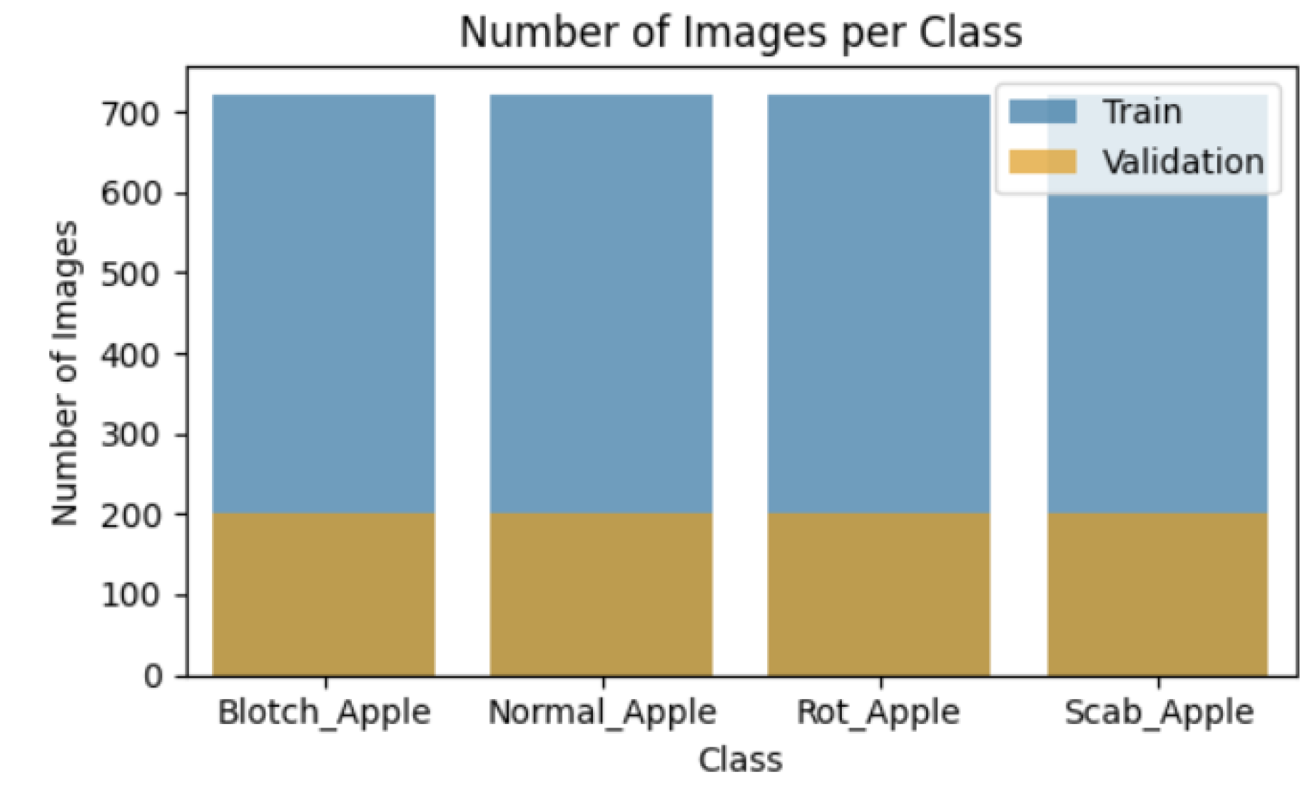
Figure 9.
Training and Validation Accuracy

6.3. Training and Validation Loss
The model’s training and validation loss across ten epochs is displayed in Figure 10. The descending trend suggests that the model is successfully capturing patterns in the training data. The train loss decreases steadily during the epochs, beginning at 0.5 and gradually reaching zero. The observation that the prediction error dramatically drops suggests that the model is doing well on the training set. Validation loss, on the other hand, demonstrates high volatility at the outset, starting at roughly 1.5, peaking significantly to around 7.0 by epoch 1, and then rapidly dropping. Although the validation loss stabilizes after epoch 2, it stays larger than the training loss and oscillates somewhat during the subsequent epochs. The model’s ability to generalize to new, untested data and avoid overfitting is indicated by the convergence of the training and validation losses.
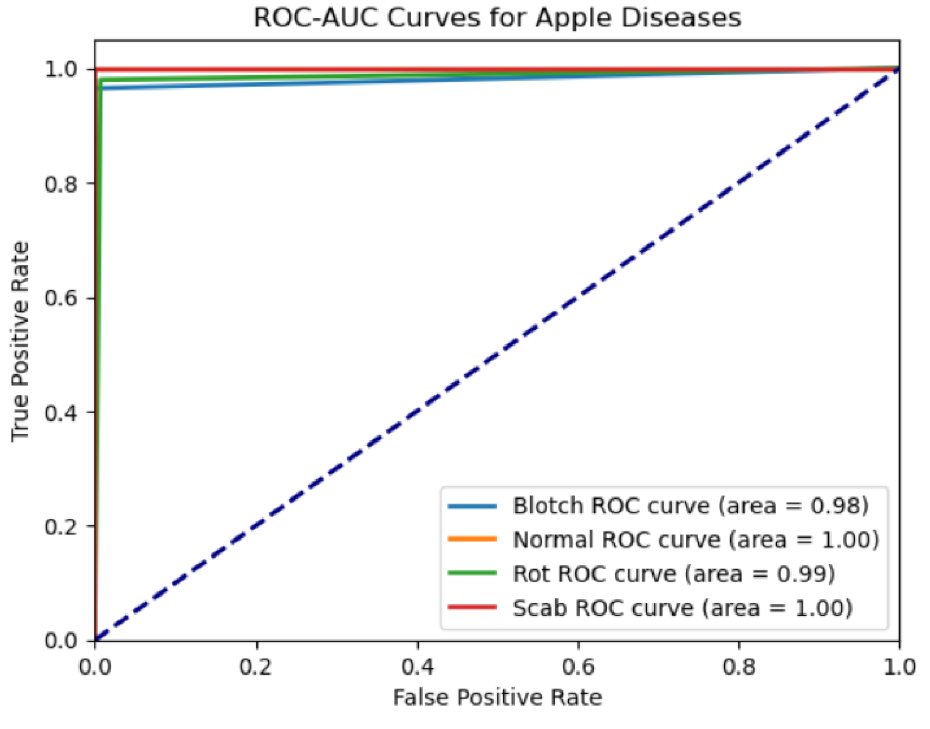
6.4. ROC-AUC Curve
When a binary classifier’s discrimination threshold varies, its diagnostic efficacy is shown on the Receiver Operating Characteristic (ROC) curve. The true positive rate (sensitivity) and the false positive rate (specificity) are analyzed [32]. The ROC of a multi-class classifier for identifying several apple diseases, such as blotch apple, healthy apple, rot apple, and scab apple, is shown in Figure 11. A comparison is made between the True Positive Rate (sensitivity) and the False Positive Rate to show how well the classifier can differentiate between apples that are infected and those that are not. The discriminative ability of the model is evaluated by the area under the ROC curve (AUC), where larger AUC values denote better performance. According to the data shown in Figure 11, the AUC for a healthy apple is 1.00, whereas that of a rot, scab, and blotch apple is 0.99, 0.98, and 1.00, respectively. These findings indicate that the model is extremely good in classifying apple diseases, with AUC values close to one and near-perfect classification performance across all categories. The ROC curves are closely packed, demonstrating constant high performance across all diseases categories.
Figure 10.
Training and Validation Loss
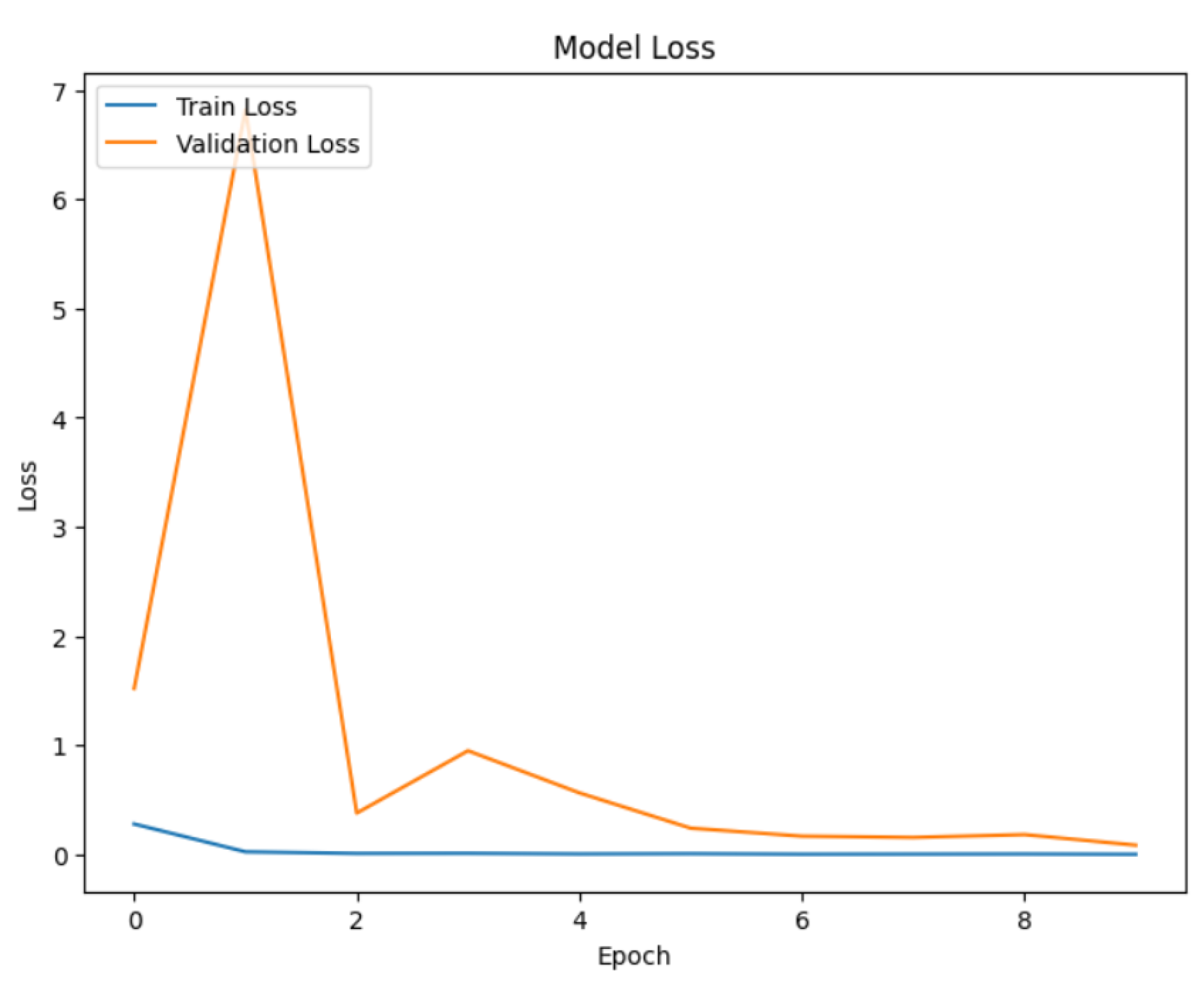
Figure 11.
ROC Curve for Apple fruit disease
6.5. PR-Curve
The Precision-Recall (PR) curve demonstrate how a classification model balances precision and recall at different probability thresholds. This curve is an effective tool for assessing the effectiveness of multi-class classification algorithms, especially when dealing with imbalanced datasets. The precision and recall of the apple disease classification model are shown for a number of categories, including blotch, healthy, rot, and scab apples, in Figure 12. Recall is the percentage of real positives found among all real positives, whereas precision is the percentage of true positives among all predicted positives. As memory improves, the curve aids in determining the trade-off between these two metrics. With AUC values of 1.00 for healthy apple, 0.99 for rot apple, 1.00 for scab apple, and 0.98 for blotch apple, Figure 12 show that the model maintains a high degree of precision and recall across all categories. AUC values near to 1 indicate that the model is highly successful in disease identification, with few false positives and strong generalization across disease categories. The findings show a high level of performance consistency across the PR curves for each condition.
6.6. Calibrated Curve for Evaluation
Figure 13, Figure 14, Figure 15, and Figure 16 show calibration curves for blotch, normal, rot, and scab apple diseases. This may assess how well the model’s predicted probabilities correspond with the actual outcomes by comparing each figure’s anticipated probability of a classifier to the actual outcomes.
Figure 12.
PR Curve for Apple fruit disease
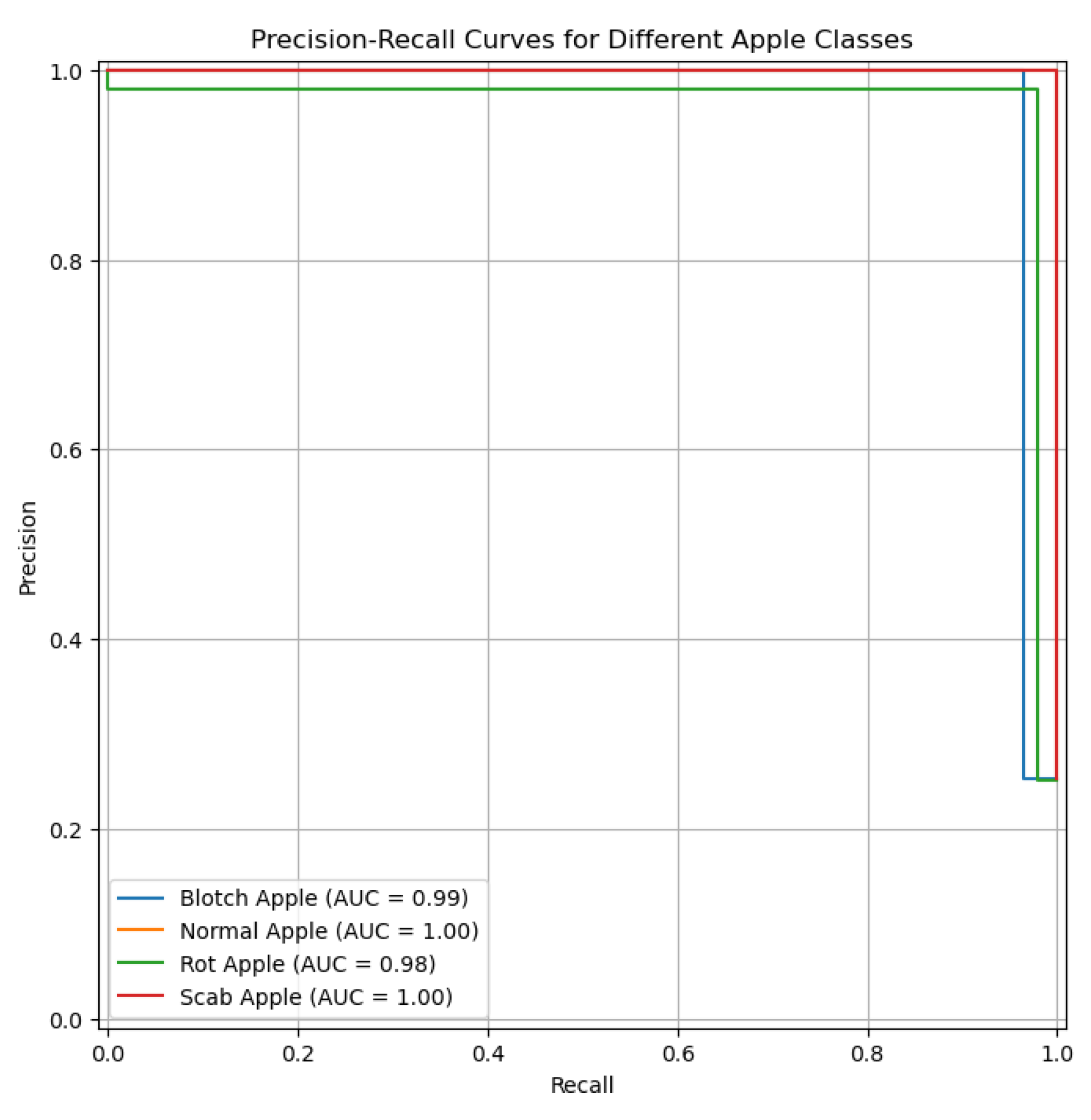
Figure 13.
Calibrated Curve for Blotch Apple
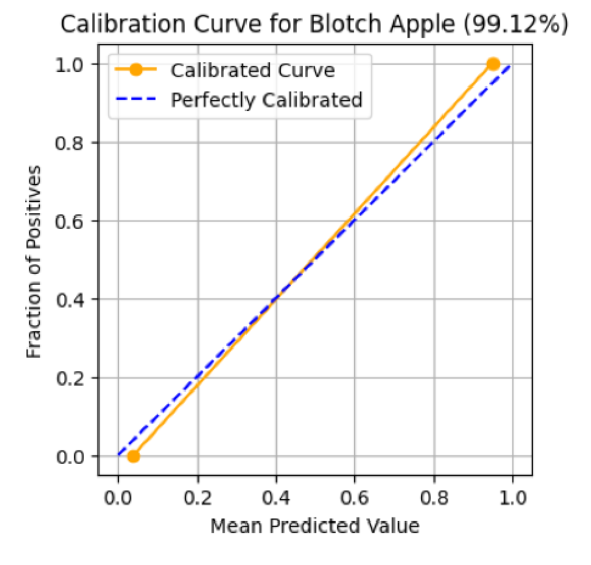
6.7. Robustness and Generalization
The approach was put to test on a dataset that included several apple diseases, including blotch, scab, and rot Apple. The analysis demonstrated how well the model could classify different diseases and identify affected areas on apples. Figure 17, Figure 18, Figure 19, and Figure 20 depict the results of blotch, rot, scab, and normal apple, respectively.
6.8. Inference Speed and Utilization
CPU Usage: The CPU usage stands at 66.60MB. While this indicates a moderate demand for CPU resources, it reflects the computational efforts required for inference. This level of usage is reasonable for ensuring swift processing without overwhelming the CPU, facilitating real-time applications.
GPU Usage: Notably, the GPU usage remains at 0.00MB, indicating that the model performs inference without relying on GPU resources. This is advantageous in environments with limited GPU availability or where minimizing GPU-related costs is a priority.
Overall, the model exhibits efficient resource management, characterized by low memory usage and moderate CPU demand. This removes the need for GPU support and making it ideal for real-time applications and deployment in a variety of contexts.
6.9. Confusion Matrix
The real labels are on the vertical axis of the Confusion Matrix, which is a square grid with the expected labels on the horizontal. The number of instances categorized with a particular combination of true and expected labels is shown in each column of the matrix. A confusion matrix showing the effectiveness of a classification model for the four types of apple diseases blotch apple, normal apple, rot apple, and scab apple is shown in Figure 21. The matrix shows the number of instances in each disease category blotch apple, normal apple, rot apple, and scab apple that were correctly diagnosed (diagonal elements) and improperly categorized (off-diagonal components).
Figure 14.
Calibrated Curve for Normal Apple
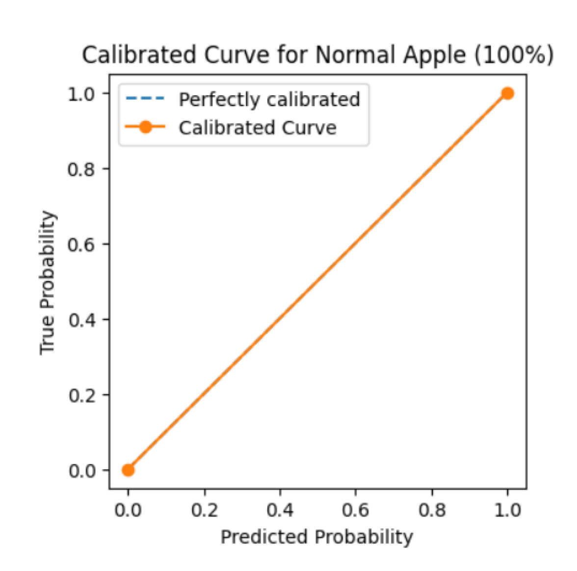
Figure 15.
Calibrated Curve for Rot Apple
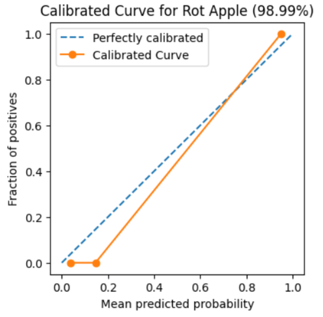
6.10. Comparison wise Results of HMAFDD
The effectiveness of the presented technique for classifying Blotch Apple, Normal Apple, Rot Apple, and Scab Apple diseases is shown in Figure 22, Figure 23, and Figure 24. The three crucial performance metrics—precision, recall, and F1-Score—are given in this section and are all stated as percentages (%). The precision of the model is the degree to which it can accurately distinguish positive cases—like diseased apples—from those that are projected to be positive. The model’s recall measures how well it can recognize every positive example. The F1-Score offers a fair assessment of the model’s overall performance and is calculated as the harmonic mean of Precision and Recall. The values of these matrices are displayed in percentage form in Table 6.
6.11. Formulae for Positive Matrices
6.11.1. Accuracy
One of the main matrics used to evaluate the performance of the model is accuracy. The proportion of correctly predicted occurrences relative to all instances in the dataset is computed. [37] is the definition of accuracy in mathematics.
Figure 16.
Calibrated Curve for Scab Apple
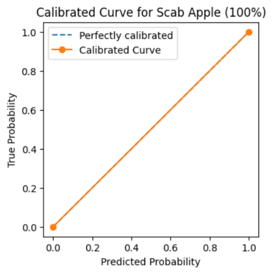
Figure 17.
Result of Blotch Apple
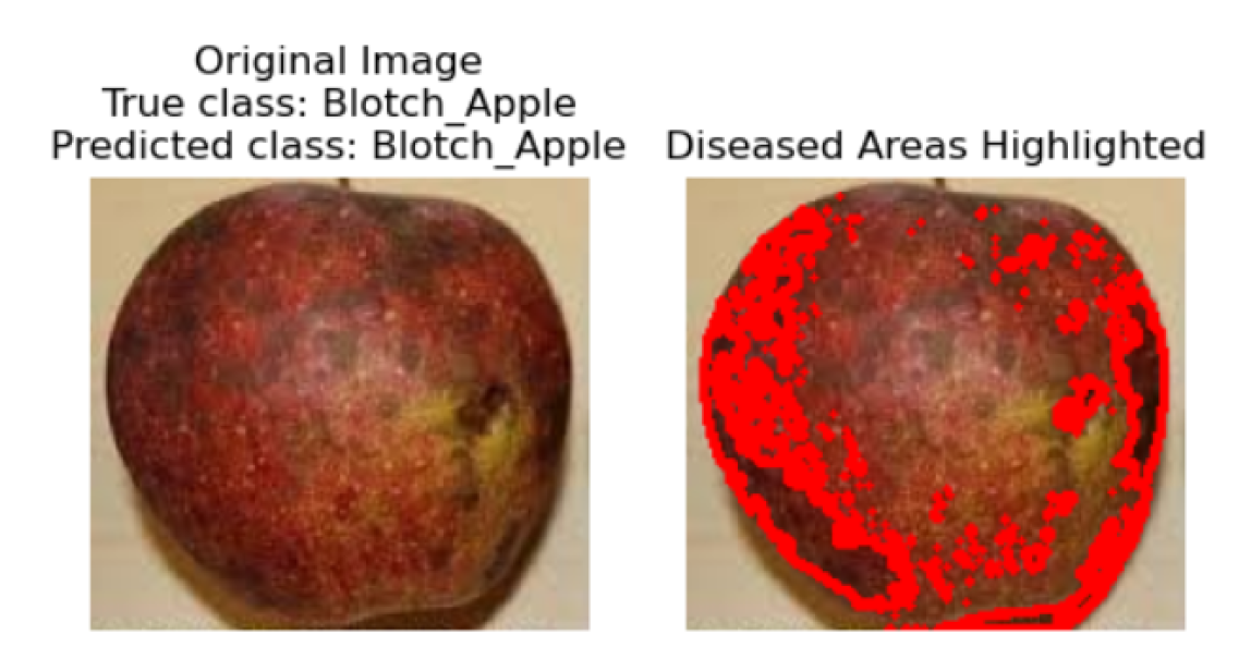
6.11.2. Precision
Another important metric for assessing model performance is precision, particularly in situations when there are class imbalances. The percentage of correctly expected positive events among all instances projected as positive is known as precision. The definition of precision in mathematics is [38].:
A greater precision suggest that the model is better at reducing false positives, which is important in situation where the false positive prediction is costly.
6.11.3. Sensitivity (Recall)
Recall, another name for sensitivity, is a crucial metric of how well the model can accurately predict good results. It measures the percentage of actual positive outcomes that the model accurately predicts. The mathematically definition of sensitivity is [39]:
A greater sensitivity score implies that the model is better at recognizing positive outcomes, which is important in situations where missing positives (false negatives) might have major consequences.
6.11.4. Specificity
One important parameter to assess the model’s accuracy in identifying negative cases is specificity. It quantifies the fraction of real negative incidents predicted properly by the model. The mathematical definition of specificity is [40].:
When misclassifying negative instances as positive might result in undesirable results, a greater specificity score suggests that the model is successful at reducing false positives. A greater specificity score implies that the model is good at reducing false positives, which is critical in situations where misclassifying negative occurrences as positive might result in undesired results.
Figure 18.
Result of Rot Apple
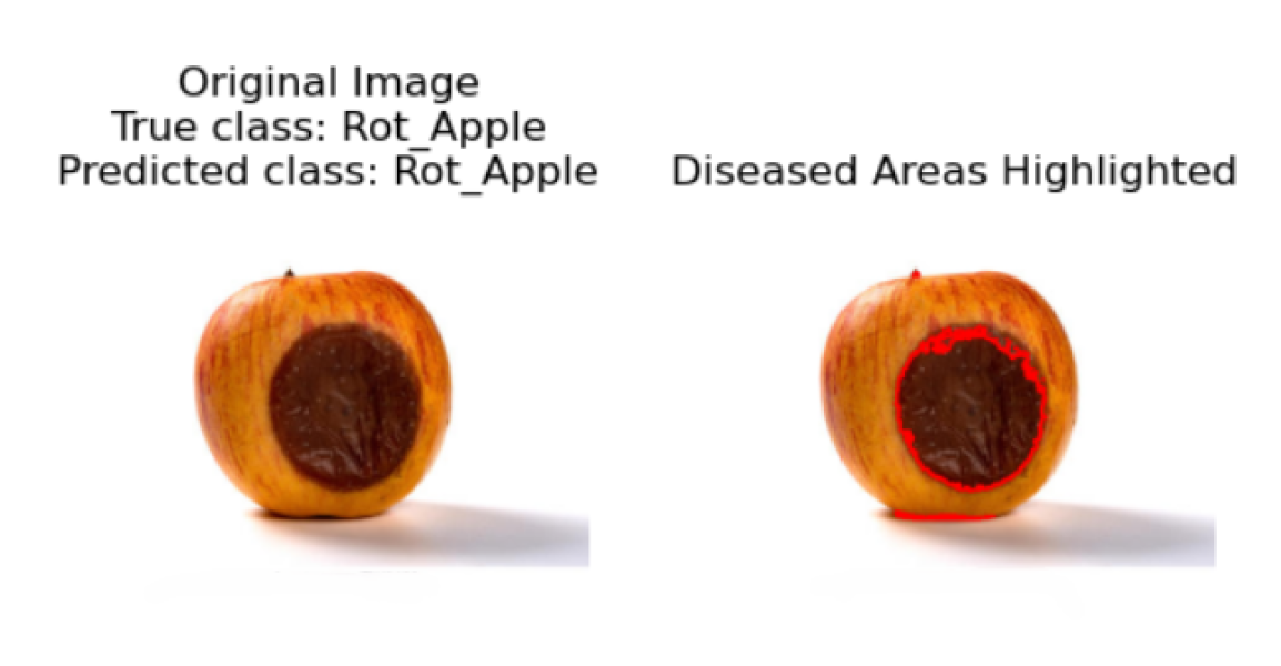
Figure 19.
Result of Scab Apple
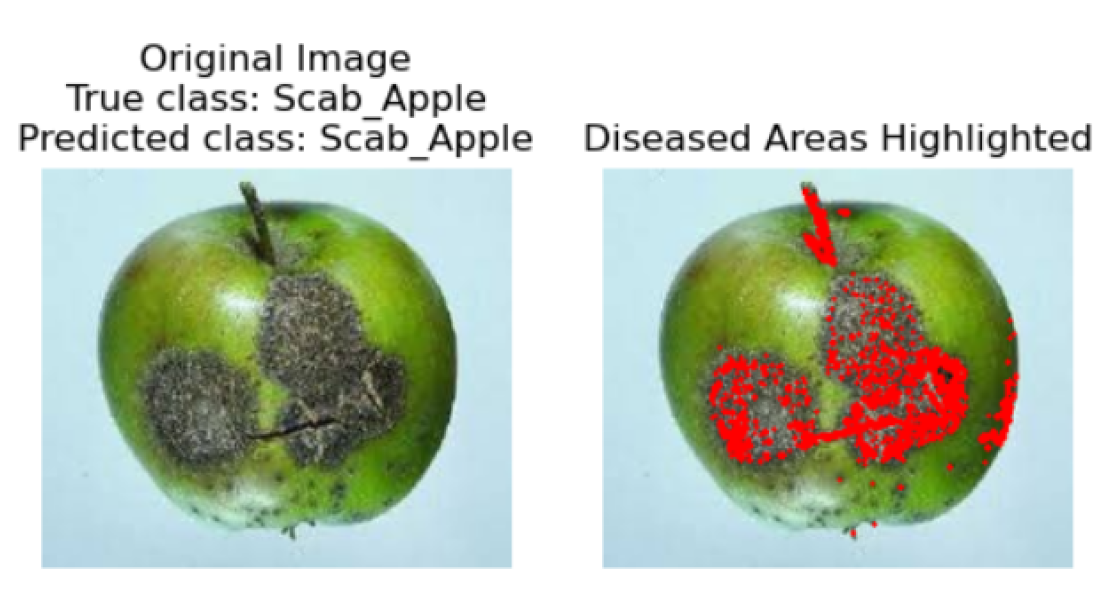
6.12. Formulae for Negative Metrices
6.12.1. False Discovery Rate (FDR)
An essential metric for evaluating the fraction of incorrect positive predictions among all the positive predictions the model produces is the False Discovery Rate (FDR). It calculates the probability that a proedicted positive occurrence is really negative. Mathematically, FDR is defined as [41]:
A lower false positive rate (FDR) indicates that the model is more effective in predicting positive outcomes, which minimizes the probability of inaccurately classifying negative events as positive. This is especially crucial in where false positive predictions can lead to significant negative consequences.
6.12.2. False Negative Rate (FNR)
To find out what fraction of real positive outcomes the model mispredicted as negative, the False Negative Rate (FNR) is a crucial metric. It estimates the model’s chance of missing that a true positive case is missed by the model. Mathematically, FNR is defined as [42]:
A lower FNR suggest that the model is more effective at recognizing positive outcomes, resulting in reducing the number of missed positive cases. This metric is particularly crucial in applications where failing to detect positive instances (false negatives) can have serious implications.
6.12.3. False Positive Rate (FPR)
An important indicator that evaluates the fraction of real negative outcomes that the model mistakenly forecasted as positive is called the False Positive Rate (FPR). It evaluates the possibility that a truly negative situation may be mistakenly identified as positive. Mathematically, FPR is defined as [43]:
A lower FPR shows that the model is better at recognizing negative instances, reducing the number of false positives. This metric is essential in applications where false positive predictions can lead to unnecessary actions or costs.
Figure 20.
Result of Blotch Apple
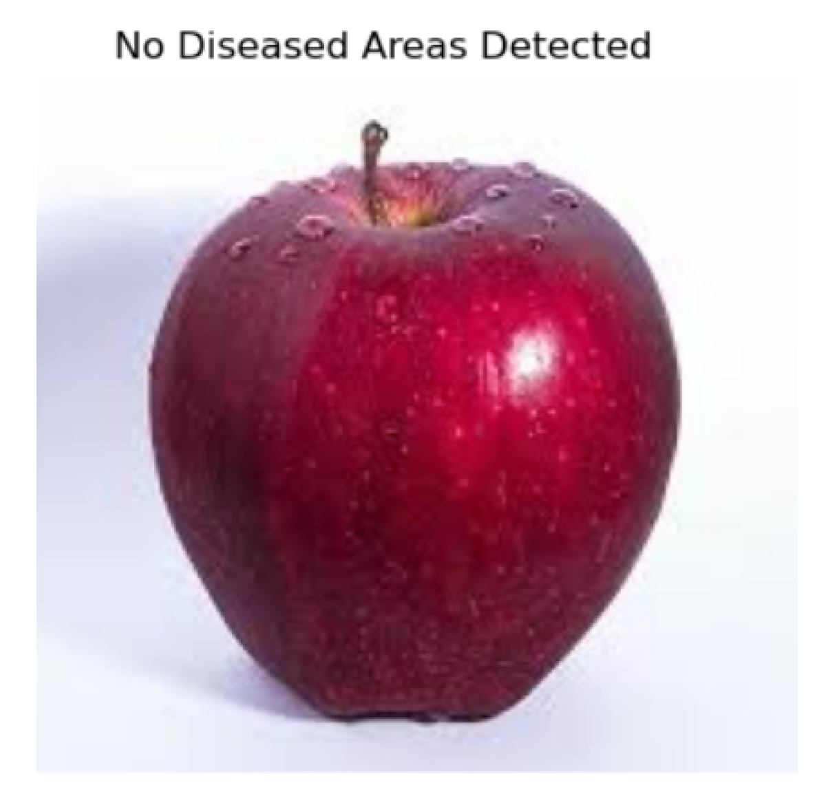
Figure 21.
Confusion Matrix of Hybrid Apple Fruit Disease Detection
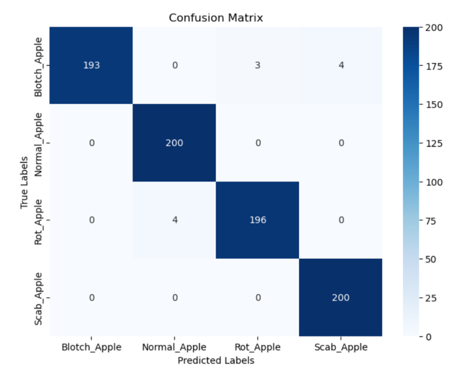
6.12.4. False Omission Rate (FOR)
An indicator of the percentage of real positive cases that the model mispredicted as negative is called the False Omission Rate (FOR). It represent the chance that a real positive case is missed, implying that the model fails to detect a positive outcomes when it should have. Mathematically, FOR is defined as [44]:
A lower FOR suggests that the model perform better at properly recognizing positive instances and avoiding missed detections. This metric is particularly important in applications where failing to detect positive cases (false omissions) can have significant consequences.
6.13. Formulae for Other Metrices
6.13.1. F-Measure
The F-Measure, often referred to as the F1-Score, is a composite measure that sums together recall and precision to provide a single score that indicates the overall performance of the model. It works especially well when testing models on imbalanced datasets and dealing with both false positives and false negatives. The F-Measure can be expressed mathematically as [45]:
By calculating their harmonic mean, the F-Measure provides a compromise between precision and recall, providing a comprehensive assessment of the model’s accuracy in identifying positive cases. A higher F-Measure indicates a more optimal recall and precision ratio.
Figure 22.
Comparison wise Result with Positive Matrices
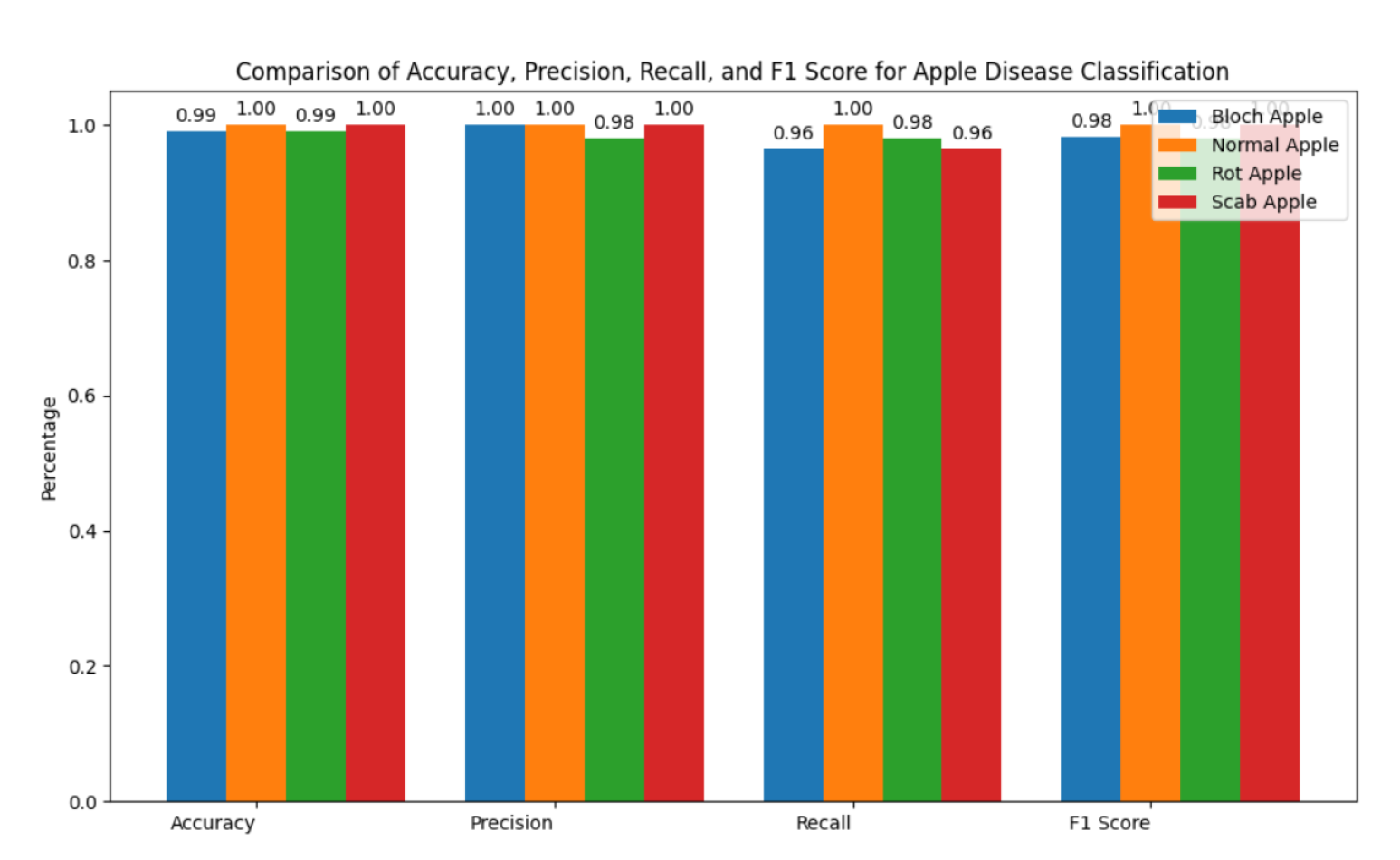
Figure 23.
Comparison wise Result with Other Matrices
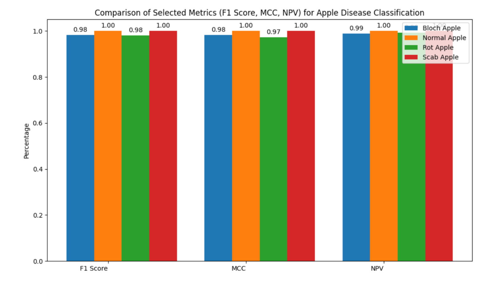
6.13.2. Matthews Correlation Coefficient (MCC)
A metric that provides an accurate evaluation of the model’s performance by taking into consideration false positives, false negatives, true positives, and true negatives is the Matthews Correlation Coefficient (MCC). Testing classification models on imbalanced datasets is very helpful. The mathematical definition of the MCC is [46]:
The MCC is a number between -1 and 1, where 1 denotes an accurate prediction, 0 denotes a predictions that is no better than chance, and -1 denotes a total disagreement between the prediction and the actual observation. Because MCC produces a single result that takes into account all four confusion matrix categories, it is highly recognized for its ability to manage imbalanced datasets. The MCC for every class was found in this study in order to evaluate the overall effectiveness of the approach. The model demonstrated its ability to balance the contributions of true positives, true negatives, false positives, and false negatives by achieving an overall MCC of X. When paired with other metrics like recall, accuracy, and precision, the MCC provides a comprehensive assessment of the model’s performance.
6.13.3. Negative Predictive Value (NPV)
The percentage of real negative results that the model accurately predicted to be negative is called the Negative Predictive Value, or NPV. It reflects the likelihood that a predicted negative instance is truly negative. Mathematically, NPV is defined as [47]:
A greater NPV shows that the model is better at recognizing negative instances, reducing the incorrect negative predictions. This metric is especially significant in scenarios when accurate identification of negative cases is required. In this study, the NPV for each class was determined to assess the model’s ability to predicting negative outcomes. The model achieved an overall NPV of X%, indicating its ability to accurately categorize negative situations while reducing false negatives. In order to provide a comprehensive assessment of the model’s classification abilities NPV is typically used in conjunction with other metrics like sensitivity, specificity, and precision. This is especially true in scenarios where the precision of negative predictions is crucial.
Figure 24.
Comparison wise Result with Negative Matrices
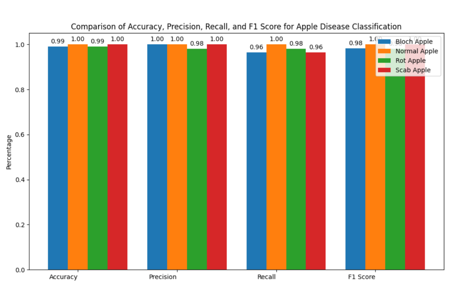
Table 6.
Comparison wise Results of HMAFDD
| Diseases | Accuracy | Precision | Recall | F-1 Score | Speci. | MCC | NPV | Actual/classified |
|---|---|---|---|---|---|---|---|---|
| Blotch | 99.12% | 100% | 96.5% | 98.2% | 100% | 98.2% | 98.8% | 193/200 |
| Normal | 100% | 100% | 100% | 100% | 100% | 100% | 100% | 200/200 |
| Rot | 98.99% | 98.0% | 98.0% | 98.0% | 99.3% | 97.3% | 99.3% | 196/200 |
| Scab | 100% | 100% | 100% | 100% | 100% | 100% | 100% | 200/200 |
6.14. Comparison of HMAFDD with Previous Work
The literature reveals a variety of methodologies for fruit disease detection, each with distinct approaches. For instance, some studies have explored CNN, DenseNet121, transformer-based models combined with CNNs for feature extraction, while others have utilized hybrid models like Deep Spectral GANs and DenseNet Recursive CNNs to enhance detection accuracy through sophisticated preprocessing, segmentation, and classification techniques. These methods, which involve preprocessing techniques like scaling, resizing, and normalizing, together with the use of deep learning models like CNNs, Vision Transformers, and DenseNet architectures, have shown effective in identifying diseases across a variety of fruit varieties. In comparison, our proposed method introduces a unique hybrid model that leverages the strengths of three pre-trained CNNs—ResNet50, DenseNet121, and EfficientNetB0. Unlike the existing methods, which rely on single or dual-model frameworks, our approach aggregates features from multiple models to create a more comprehensive feature vector. This aggregation is further refined through global average pooling and concatenation, ensuring the model captures a wider range of relevant features. Additionally, while regularization techniques like dropout are commonly employed in other studies, our model also incorporates advanced training strategies, such as EarlyStopping and ReduceLROnPlateau, to optimize training dynamics and prevent overfitting. Finally, the classification process is streamlined using a softmax activation function, ensuring a clear and accurate prediction of the disease class. This multi-phase, hybrid method enables our model to outperform existing literature in terms of feature richness, robustness, and classification accuracy, notably for apple disease detection. The Comparison Graph comparing our proposed system (HAMFDD) to the existing system is shown in Figure 25. and the values of model performance are displayed in Table 7.
Figure 25.
Comaprsion Graph with previous work and Hybrid Apple Disease Detection
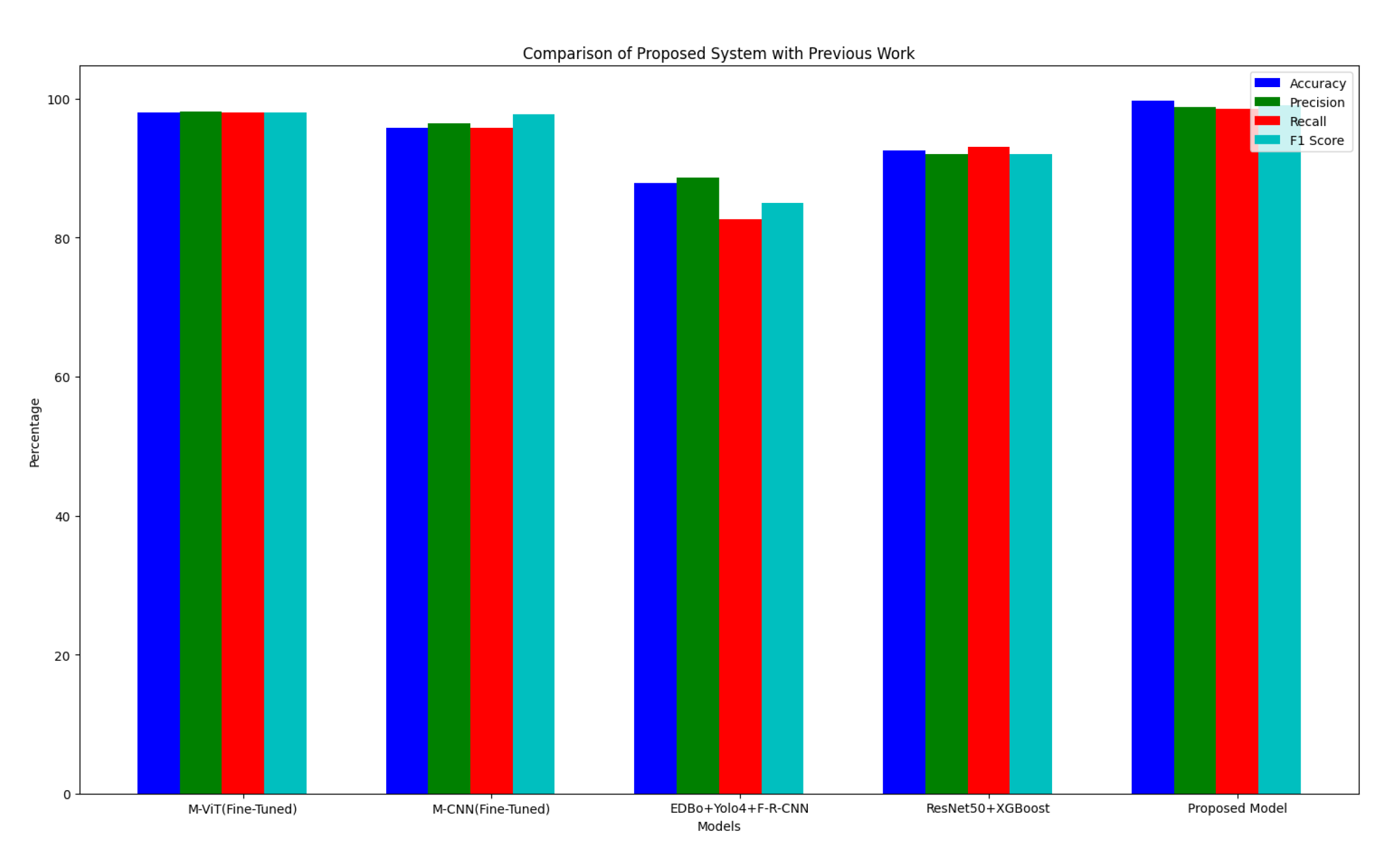
Table 7.
Performance Metrics of Different Models
| Model | Year | Accuracy | Precision | Recall | F-1 Score |
|---|---|---|---|---|---|
| Modified ViT(Fine-Tuned) [11] | 2024 | 98.05% | 98.08% | 98.05% | 98.03% |
| Modified CNN(Fine-Tuned) [11] | 2024 | 95.77% | 96.44% | 95.77% | 97.79% |
| EfficientDetBo+Yolo4+Faster R-CNN [12] | 2022 | 87.9% | 88.6 | 82.6% | 85% |
| ResNet50+XGBoost [13] | 2022 | 92.48% | 92.00% | 93.00% | 92.00% |
| HMAFDD | 2024 | 99.52% | 98.75% | 98.5% | 99.0% |
7. Patents
This section is not mandatory, but may be added if there are patents resulting from the work reported in this manuscript.
Funding
No Funds were obtained to help with the development of this paper.
Data Availability Statement
Abbreviations
The following abbreviations are used in this manuscript:
| HMAFDD | Hybrid Model for Apple Fruit Disease Detection |
| DCNN | Deep Convolutional Neural Network |
| CNN | Convolutional Neural Network |
| Grad-CAM | Gradient-weighted Class Mapping |
| GLCM | Gray Level Co-occurance Matrix |
| SSAP | Spectral-shifted Adversarial Perturbation |
| ARR | Adaptive Region-Based Resizing |
| CACN | Context-Aware Contrast Normalization |
| DADP | Diseased-Aware Dynamic Padding |
| TP | True Positives |
| TN | True Negatives |
| FP | False Positives |
| FN | False Negatives |
References
- Khan, M. A. et al. An optimized method for segmentation and classification of apple diseases based on strong correlation and genetic algorithm based feature selection. IEEE Access 7, 46261–46277 (2019). [CrossRef]
- Kukreja, V. & Dhiman, P. A deep neural network based disease detection scheme for citrus fruits. 2020 International conference on smart electronics and communication (ICOSEC) 97–101 (2020). [CrossRef]
- Vishnoi, V. K., Kumar, K., Kumar, B., Mohan, S. & Khan, A. A. Detection of apple plant diseases using leaf images through convolutional neural network. IEEE Access 11, 6594–6609 (2022).
- Alharbi, A. G. & Arif, M. Detection and classification of apple diseases using convolutional neural networks. 2020 2nd international conference on computer and information sciences (ICCIS) 1–6 (2020).
- Patel, H. B. & Patil, N. J. An intelligent grading system for automated iden- tification and classification of banana fruit diseases using deep neural network. International Journal of Computing and Digital Systems 15, 761–773 (2024).
- Gu, Y. H. , Yin, H., Jin, D., Zheng, R. & Yoo, S. J. Improved multi-plant disease recognition method using deep convolutional neural networks in six diseases of apples and pears. 2022; 12. [Google Scholar]
- Safari, Y., Nakatumba-Nabende, J., Nakasi, R. & Nakibuule, R. A review on automated detection and assessment of fruit damage using machine learning. IEEE Access (2024).
- W¨ohner, T. & Emeriewen, O. F. Apple blotch disease (marssonina coronaria (ellis & davis) davis)–review and research prospects. European journal of plant pathology 153, 657–669 (2019).
- Shafi, S. M. et al. An overview of apple scab, its cause and management strategies. EC Microbiol 15, 1–4 (2019).
- Lyousfi, N. et al. Combination of sodium bicarbonate (sbc) with bacterial antag- onists for the control of brown rot disease of fruit. Journal of Fungi 8, 636 (2022).
- Zala, S., Goyal, V., Sharma, S. & Shukla, A. Transformer based fruits disease classification. Multimedia Tools and Applications 1–21 (2024).
- Khan, A. I., Quadri, S. M. K., Banday, S. & Latief Shah, J. Deep diagnosis: A real-time apple leaf disease detection system based on deep learning. Comput. Electron. Agric. 198, 107093 (2022).
- Buyukarikan, B. & Ulker, E. Classification of physiological disorders in apples fruit using a hybrid model based on convolutional neural network and machine learning methods. Neural Comput. Appl. (2022).
- Sottocornola, G., Baric, S., Nocker, M., Stella, F. & Zanker, M. DSSApple: A hybrid expert system for the diagnosis of post-harvest diseases of apple. Smart Agricultural Technology 3, 100070 (2023).
- Subha, V. & Kasturi, K. A comparative stratification of automated indaga- tion on apple disease using DeepSpectral generative adversarial and densenet convolutional neural network 1–6 (2024).
- Sumanto et al. Model na¨ıve bayes classifiers for detection apple diseases 1–4 (2021).
- Alharbi, A. G. & Arif, M. Detection and classification of apple diseases using convolutional neural networks 1–6 (2020).
- Li, X. & Rai, L. Apple leaf disease identification and classification using resnet models, 738–742 (IEEE, 2020).
- Zhang, X. et al. Classification and identification of apple leaf diseases and insect pests based on improved resnet-50 model. Horticulturae 9, 1046 (2023).
- Swaminathan, A., Varun, C., Kalaivani, S. et al. Multiple plant leaf disease classification using densenet-121 architecture. Int. J. Electr. Eng. Technol 12, 38–57 (2021).
- Haider, I., Khan, M. A., Nazir, M., Kim, T. & Cha, J.-H. An artificial intelligence- based framework for fruits disease recognition using deep learning. Computer Systems Science & Engineering 48 (2024).
- Bansal, P., Kumar, R. & Kumar, S. Disease detection in apple leaves using deep convolutional neural network. Agriculture 11, 617 (2021).
- Turkoglu, M., Hanbay, D. & Sengur, A. Multi-model lstm-based convolutional neural networks for detection of apple diseases and pests. Journal of Ambient Intelligence and Humanized Computing 13, 3335–3345 (2022).
- Li, L., Zhang, S. & Wang, B. Plant disease detection and classification by deep learning—a review. IEEE Access 9, 56683–56698 (2021).
- Ayaz, H. et al. Classification of apple disease based on non-linear deep features. Applied Sciences 11, 6422 (2021).
- Pandian, J. A. et al. Plant disease detection using deep convolutional neural network. Applied Sciences 12, 6982 (2022).
- Rajeena PP, F., SU, A., Moustafa, M. A. & Ali, M. A. Detecting plant disease in corn leaf using efficientnet architecture—an analytical approach. Electronics 12, 1938 (2023).
- Marandi, S. & Chakravorty, C. Apple fruit disease detection using image processing. Journal of Emerging Tech. and Innovative Research (JETIR) 8 (2021).
- Yadav, A. et al. Afd-net: Apple foliar disease multi classification using deep learning on plant pathology dataset. Plant and Soil 477, 595–611 (2022).
- Jain, S., Seth, G., Paruthi, A., Soni, U. & Kumar, G. Synthetic data augmentation for surface defect detection and classification using deep learning. Journal of Intelligent Manufacturing 1–14 (2022).
- Islam, M. A. et al. Machine learning based image classification of papaya disease recognition, 1353–1360 (IEEE, 2020).
- Kutyrev, A., Kiktev, N. A., Kalivoshko, O. & Rakhmedov, R. S. Recognition and classification apple fruits based on a convolutional neural network model., 90–101 (2022).
Figure 5.
Modeling of Apple Fruit Disease based Hybrid Deep Learning Approach
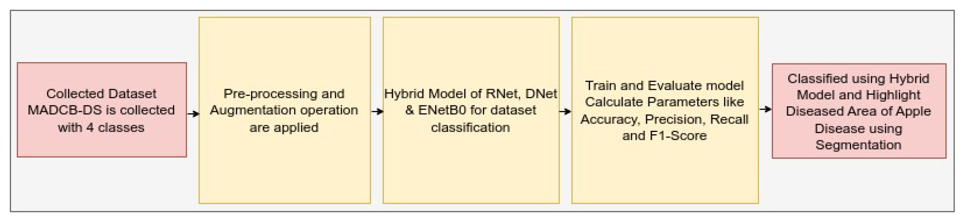
Table 2.
Class Label of Apple diseases
| Apple Diseases | Label |
|---|---|
| Blotch_Apple | 0 |
| Normal_Apple | 1 |
| Rot_Apple | 2 |
| Scab_Apple | 3 |
Table 3.
Data partitioning of original images for training and validation
| Dataset | Total Samples | Training samples | Validation samples |
|---|---|---|---|
| Healthy | 91 | 67 | 24 |
| Unhealthy | 411 | 315 | 96 |
Table 4.
Data partitioning after applying data augmentation on original images for training and validation
Table 4.
Data partitioning after applying data augmentation on original images for training and validation
| Dataset | Total Samples | Training samples | Validation samples |
|---|---|---|---|
| Healthy | 920 | 720 | 200 |
| Unhealthy | 2760 | 2160 | 600 |
Disclaimer/Publisher’s Note: The statements, opinions and data contained in all publications are solely those of the individual author(s) and contributor(s) and not of MDPI and/or the editor(s). MDPI and/or the editor(s) disclaim responsibility for any injury to people or property resulting from any ideas, methods, instructions or products referred to in the content. |
© 2024 by the authors. Licensee MDPI, Basel, Switzerland. This article is an open access article distributed under the terms and conditions of the Creative Commons Attribution (CC BY) license (http://creativecommons.org/licenses/by/4.0/).
Copyright: This open access article is published under a Creative Commons CC BY 4.0 license, which permit the free download, distribution, and reuse, provided that the author and preprint are cited in any reuse.


