Submitted:
25 March 2025
Posted:
26 March 2025
You are already at the latest version
Abstract
China is the world's largest producer of chili peppers, which occupy particularly important economic and social values in various fields such as medicine, food and industry.However, during its production process, chili peppers are affected by pests and diseases resulting in significant yield reduction due to temperature, environment and other reasons. In this study, a lightweight pepper disease identification method DD-YOLO based on the YOLOv8n model is proposed. First, the deformable convolutional module DCNv2 (Deformable Convolutional Networks) and the inverted residual mobile block iRMB (Inverted Residual Mobile Block) are introduced into the C2Fmodule to improve the accuracy of the sampling range and reduce the computational amount; secondly, the DySample sampling operator (Dynamic Sample) is integrated into the head network toreduce the amount of data and reduce the complexity of computation. Finally, we use Large Separable Kernel Attention (LSKA) to improve the SPPF module (Spatial Pyramid Pooling Fast) to enhance the performance of multi-scale feature fusion. The experimental results show that the accuracy, recall and average precision of the DD-YOLO model are 91.6%, 88.9% and 94.4%, respectively, compared with the base network YOLOv8n, it improves 6.2, 2.3 and 2.8 percentage points respectively, the model weight is reduced by 22.6%, and the number of floating-point operations per second is improved by 11.1%. This method provides a technical basis for intensive cultivation and management of chili peppers as well as efficiently and cost-effectively accomplishes the task of identifying chili pepper pests and diseases.
Keywords:
pepper
; disease image recognition
; YOLOv8
; sampling operator
; deformable convolution
; inverse residual shift
1. Introduction
As the world’s top three fruits and vegetables, chili peppers rank first in the world interms of planting area and production in China. It has a unique diversity of values such as edible, medicinal, ornamental, etc. But at present, the high morbidity rate and the difficulty of monitoring the initial stage of the disease during the production process have become the key factors restricting the chili pepper industry. So it is crucial to implement effective measures for the prevention, control, and management of chili pepper diseases and pests [1]. In recent years, with the development of computer technology and the wide application of artificial intelligence, traditional agriculture has been developing towards intelligence and modernization [2]. The shift of which provides a developing direction for the intensive cultivation of fruits and vegetables. Meanwhile, the real-time target pest monitoring can provide intelligent and modernized solutions for the growth process of chili peppers [3]. Besides, the rapid detection of chili peppers’ pests and diseases based on the target recognition has an important practical significance for the stability of its yield and the increase of its yield.
With the rocketing development of computer technology, the non-contact target detection technology of computer vision with crops as the main body provides the technical basis for crop intensive management. Two-stage improved RCNN is widely used in crop target detection. Su, T et al. [4]constructed a wheat leaf pest and disease identification model by replacing Softmax with an improved Local Vector Machine (LSVM) as the model classifier to improve the classification ability of the model. It was verified to have an average identification accuracy of 93.68% through experiments. Xi, R et al. [5] Res- 51 NET50 was used as the backbone network of RCNN to construct a potato sprout detection model to improve the recognition ability of multi-scale features, and the model was verified through experiments to have an average recognition accuracy of 97.71%, which was 54 5.98% higher compared to the original model. Li, Y et al. [6] introduced methods of an improved Shallow Neural Network SCNN-KSVM (Shallow CNN with Kernel SVM) and SCNN-RF (Shallow CNN with Random Forest) to construct a shallow and efficient crop disease model, which was experimentally verified to have an average recognition accuracy of 94%, with a thousand-fold reduction in the number of parameters compared with other traditional deep convolutional neural networks [6]. By introducing transfer learning in CNN, Pattnaik, Gayatri et al. [7]. has constructed a tomato plant pest classification model. This method enhances the model’s ability to recognize multi-scale features. Experimental results show that the model achieves an average recognition accuracy of 88.83%, representing an improvement of 11.63% compared with the original model.
Although the Two-stage algorithm can provide higher detection accuracy, the number of parameters is larger and more computationally expensive. Another One-stage model based on SSD and YOLO is faster and less computationally expensive. Liu,J et al. [8]improved the YOLOv3 model by pooling pyramid layer fusion of multiscale features, constructed a tomato pest detection model to improve the recognition rate of small feature targets, and verified that the average recognition accuracy of this model has reached 92.39% through experiments. Han Xin et al. [8] constructed a disease identification model by using CSPD-arknet as the backbone feature extraction network and replacing the SPD-Convmodule with stride-2 convolution, which further improved the speed of feature extraction while guaranteeing the accuracy due to the introduction of the SE mechanism. The average identification accuracy of the model has reached 95.7%, regarded as a great reduction in the weight of the model compared with that of the original network. Jinming Zheng et al. [9] improved YOLOv8 by introducing the Convolutional Block Attention Module(CBAM) and replacing the Conv in the neck with Ghost, and constructed the cabbage size prediction model YOLOv8n-CK, which was verified to have an average recognition accuracy of 99.2%, and the floating-point operations per second were reduced by 13.04% comper pest model. [10, 11]
In recent years, machine vision has also been widely applied to the detection of phenotypic features of chili peppers. Anita S. Kini et al. [12]recognized and classified multiple pests and diseases of chili peppers by combining models, and the accuracy of the different classes of diseases could reach 60% to 90%, but the model construction process is more complicated, and it is not an end-to-end detection method, and the detection rate is slower than that of single-stage algorithms. Xuejun Yue et al. [13] improved the Yolov7 baseline model by improving GhostNetV2 to improve the backbone network, replacing the feature extraction module with CFNet, and introducing the CBAM attention mechanism, which increased the accuracy by 12% compared to the baseline model, but due to the complexity of the baseline model structure, the model still has redundancy, and it is not applicable to be deployed on the edge-enabled devices; Na Ma et al. [14] improved Yolov8n baseline model by improving GhostNetV2 to improve the backbone network, replacing the feature extraction module with CFNet and introducing the CBAM attention mechanism. The baseline model is improved by improving the backbone network as well as improving C2f and introducing CARAFE sampling operator, which improves the average detection accuracy by 2% compared to the baseline model, but there may be data leakage due to blurring of data division.
Aiming at these problems, this study, based on Yolov8n, introduces DCNv2 and iRMB in the C2f layer, proposes fusion Dysample to improve the model and proposes the LSKA attention mechanism, and proposes a pepper disease detection model, DD-Yolo, which shows a good detection effect in the small disease features and has a good improvement in the detection speed of the model size, so that the model has good detection capability on the marginalized embedded devices with good detection capability. This study not only provides technical support for pepper disease monitoring, but also promotes the development of intelligent agriculture.
2. Materials and Methods
2.1. Establishment of the Data Set
The images used in the experiment were taken in the chili pepper experimental park of Northeast Agricultural University’s Smart Agriculture, and the acquisition device was a Huawei P50 smartphone with a resolution of 1224*2700 pixels. Considering the different light conditions of the growing environment of chili peppers and the shading of their own characteristic conditions, the images were taken under different weather conditions and environmental conditions, including sunny days, after rain and field of view overlap,shading, smooth light, backlight, changing angles and distances, and so on. In order to enrich the diversity of data and improve the model generalization ability as much as possible, and to improve the recognition ability in complex environments [16]. A total of 2112images were collected, and the images of pepper disease leaves were taken as shown in Figure 1.
The experiment uses LabelImg annotation software to annotate the features of the above dataset to form a sample set, using rectangular boxes to frame all the diseased leaves in the image one by one, save the format as YOLO “txt” file, and divide the completed rice dataset into test and validation sets according to the division ratio of 9:1. The training set includes 1901 images and the validation set includes 211 images, totaling 9098 labels [12].The division results are shown in Table 1:
During real production operations, the acquisition robot end-effector moves dynamdata processing flow is shown in Figure 2.
2.2. Pepper Target Detection Methods
2.2.1. YOLOv8 Convolutional Network Modeling
YOLOv8 is a target detection algorithm introduced by Ultralytics in January 2023 for tasks such as image classification, object detection, and instance segmentation, which possesses several advantages such as higher detection performance, smaller number of model parameters, and faster inference speed, etc. It discards the previous allocation method of IoU allocation or unilateral proportion, and adopts the Task-Aligned Assigner positive negative sample allocation strategy is adopted, which significantly improves the model performance. The YOLOv8 network structure consists of four main parts: Input, Backbone, Neck and Head. The backbone network is mainly responsible for extracting image features, which can be divided into three parts: standard convolution (Conv) module, C2f module, and SPPF module. Among them, the SPPF module connects the backbone network and the neck network, extracts the pepper features through different convolution kernels, and then fuses the feature information of different scales. The standard convolution (Conv) module consists of convolutional layers, which are responsible for feature extraction from the input data, and different levels of feature information are extracted through layer-by-layer convolution. In the YOLOv8 model, the Conv layer can be adapted to different input data and detection tasks by adjusting parameters such as the size, number and step size of the convolution kernel. The SPPF module is applied between the feature extraction network (backbone) and the neck network (neck). The feature extraction network is responsible for extracting the feature information of the input image, while the neck network is responsible for fusing and integrating this feature information, effectively fusing feature information at different scales to improve the model’s ability to recognize the target [18,17,9,4] (Vijayakumar, Vairavasundaram, and Applications 2024) (Vijayakumar, Vairavasundaram, and Applications 2024) [2].
The Head network (Head) consists of a series of convolutional and anti-convolutional layers used to generate detections of diseases. Each detector consists of a set of convolutional and fully connected layers for predicting the bounding box at that scale, and each subtask is responsible for predicting the bounding box at one scale.
2.2.2. Proved DD-YOLO Algorithm
Aiming at the characteristics of pepper pests and diseases with many types and small scales, this study proposes a lightweight pepper disease recognition method DD-YOLO based on the YOLOv8n base model, firstly, by introducing DCNv2 and IRMB into the C2f module, to improve the adaptive sampling of the model; by integrating the DySample ultra-lightweight dynamic up-sampling operator in the header network, to reduce the computational volume and model complexity; by introducing the LSKA attention mechmulti-scale feature fusion capability and reduce misdetection and omission [19]. The DD-YOLO model diagram is shown in Figure 3.
1) C2f-iRBM module
The Inverted Residual Mobile Block (iRMB) combines a lightweight Convolutional Neural Network (CNN) architecture with a highly efficient Multi-Head Self-Attention(MHSA) mechanism to build a new network architecture that maintains the lightweight nature of the model while maximizing the utilization and accuracy of computational resources. iRMB is designed to significantly reduce the number of parameters and computational complexity without sacrificing model performance. The core design concept of iRMB is that the combination of these two techniques significantly reduces the number of parameters and computational complexity without sacrificing the performance of the 178 model [22]. With the same training configuration, iRMB demonstrates excellent efficacy, utilizing fewer parameters and computational resources to achieve improved performance, an advantage that is particularly significant when applied to columnar visual Transformers such as variants of ViT. Meanwhile, in the lightweight model architecture, iRMB with a single-residual structure has a more obvious performance advantage over the traditional two-residual Transformer structure [21]. In this improvement this study uses C2f-iRMB as the key feature extraction branch through optimization strategies such as transaction compression, slicing techniques, and microtransactions to reduce the data storage requirements of the model during computa-tion and alleviate the high demand on hardware resources.C2f-iRMB not only inherits the iRMB’s feature of maintaining the model’s lightness while improving its performance, but also through the enhancement characteristics of C2f, it further enhances the model’s ability to capture fine and small targets in rice disease images [22]. This design enables the network to efficiently and accurately extract key features from the images under the limited computational power environment, which effectively improves the performance and efficiency of the model in practical applications.The IRMB structural paradigm is shown in Figure 4.
2) C2f-DCNv2 module
DCNv2 is an improved version of DCNv1. DCNv2 enhances its ability to focus on relevant image regions by improving modeling capabilities and introducing stronger training strategies. c2f-DCNv2 builds on this foundation by incorporating a network specific architectural design (the CSP Bottleneck structure). at the heart of the c2f-DCNv2 module is the deformable convolutional layer, which allows the convolutional kernel to deform freely on the input feature map, thus capturing the shape of the target more accurately [24]. In order to deepen the flexibility of deformable convolutional networks in spatialsupport region processing, a tuning mechanism is introduced here. This mechanism endows the deformable convolutional network module with a dual capability: on the one hand, it dynamically adjusts the spatial offsets used to sense the input features in order to capture more precise feature location information; on the other hand, it also modulates the magnitude of feature components from different spatial locations. This feature allows the module to selectively ignore or exclude signals from these specific locations by directly setting the feature amplitude of certain location components to zero in extreme cases [23]. As a result, this spatial location selective ignoring mechanism significantly reduces the impact of the corresponding image content on the module’s output, adding a whole new dimension to the network module’s tuning of the spatial support region.The DCNv2 structure is shown in Figure 5.
where y(p0) denotes the value at position p0 on the output feature map, wk is the weight of the convolution kernel, pk is the fixed offset of the kth sampling point in the convolution kernel, Δpk is the sampling point offset , Δmk is the modulation coefficient.
𝒚(𝒑𝟎) = ∑𝒌𝐰𝒌 ∗ 𝒙(𝒑𝟎 + 𝒑𝒌 + ∆𝒑𝒌) ∗ ∆𝒎𝒌0
3) Fusion of DySample sampling operators
DySample is an ultra-lightweight and efficient dynamic upsampler. Compared to traditional kernel-based dynamic upsamplers, DySample adopts a point-based sampling approach, which solves the problem that FADE and SAPA’s need for high-resolution feature guidance has somewhat limited their application scenarios [24]. At the same time, DySample does not require custom CUDA packages and has much fewer parameters, FLOPs, GPU memory and latency than kernel-based dynamic upsamplers. Moreover, DySample outperforms other upsamplers in the prediction task of object detection.
In this study, DySample sampling operator is used to optimize the computational efficiency of the model. In the feature extraction module, the traditional sampling module is replaced by DySample operator as the main data flow branch through class inheritance to reduce the computational complexity of the model. By introducing the DySample operator, we further reduce the computation and memory occupation during the sampling process, thus realizing the lightweight of the model.The DySample structure is shown in Figure 6.
In generator (b), the sample set is the sum of the generated offsets and the original grid positions. The top figure shows the version with “static range factors”, where the offsets are generated through a linear layer. The lower figure depicts the version with “dynamic range factors”, where the range factors are first generated and then used to adjust the offsets [26]. “σ” denotes the Sigmoid function.
4) Add Attention Mechanism LSKA
LSKA improves on the Large Convolutional Kernel Attention Module (LKA) by decomposing the two-dimensional convolutional kernels of the deep convolutional layers into horizontal and vertical one-dimensional convolutions in tandem [25].The key features of LSKA include long-range dependence, spatial and channel adaptation, and scalability to very large kernels.The spatial attention and channel attention strategies employed by LSKA adaptively recalibrate the feature weights as compared to the LKA, LSKA further reduces memory and computational complexity by cascading kernels. This solves the problem of quadratic growth of computation and memory footprint when the convolutional kernel size of the deep convolutional layer increases in LKA, while maintaining adaptive and long-range correlation, and achieves performance com- 267 parable to that of the standard LKA at low computational complexity and memory foot- 268 print [25].The LSKA structure is shown in Figure 7.
In this study, LSKA is embedded into the SPPF module of YOLOv8 to improve the accuracy of pepper disease recognition and the computational efficiency of the model. Specifically, at the C2f module of feature extraction, this study introduces the LSKA attention mechanism to replace the traditional convolution operation as the main feature fusion branch in order to enhance the model’s fusion capability of multi-scale features; secondly, the feature extraction process is further refined by constructing the SPPF-LSKA module to improve the model’s recognition accuracy of pepper disease features. Through these improvements, the number of floating-point operations and computation of the model are further successfully reduced, while maintaining the efficient feature extraction performance.
2.3. Perimental Platform and Parameter Settings
In this study, all models are tested under the same conditions to ensure unbiased testing. We also include ablation experiments, where we remove or “ablate” (set the weights to zero) certain layers or parameters in the model to observe the effect on the model performance, in order to better understand the role of each layer and parameter in the network and its impact. In addition, we introduce a comparison test to compare the YOLOv8 base network, the improved network, and other target detection models to further evaluate the performance differences between the different models, thus helping us to select the most appropriate model.
This experiment was conducted under the 64-bit operating system Windows, and the detailed configuration of the server is shown in Table 2:
2.4. Analysis of the Rationality of the Model Improvement Method
2.4.1. Exmparison of Other Lightweight Model Backbone Networks
In this study, on the base network of YOLOv8, the replacement of the backbone network is carried out and the training set is trained while keeping all the parameter settings unchanged [11, 25]. In this study, the training results are compared and analyzed, and the specific comparison results are shown in Table 3.
As can be seen from Table 3, the accuracy, recall, and average precision of the model after using the C2f-iRMB improvement method are all at a high level, in which the preci- 306 sion is improved by 9.3 percentage points compared to that of the CHOSTHGNetV2 back- 307 bone network. In terms of model computing speed, C2f-iRMB is slightly lower than C2f- 308 AKConv and C2f-MSBlock, but its detection accuracy is remarkable, and the GFLOPs of the C2f-iRMB model are only slightly lower than that of C2f-AKConv by 0.2. Overall, our model improves on the inference speed while maintaining a high level of accuracy [27].
2.4.2. Visualization of C2f-DCNv2 Model Features
In order to gain a deeper understanding of the ways in which the deformable convolutional module DCNv2 enhances its recognition capabilities, we have taken the step of visualizing the operation by mapping its features, a measure that allows us to see more clearly how the key image regions on which its internal layers depend vary.
As can be observed from Figure 8, with the gradual deepening of the number of network layers, the features extracted in each layer undergo a shift from concrete to abstract. Specifically, the activation output of the initial layer retains more of the original visual content information of the image, which is gradually compressed and abstracted as the layers are incremented to focus more on category-related feature information. This demonstrates how the deformable convolutional module DCNv2 can enhance the recognition of targets by gradually building up target features [28]. The Feature map is shown in Figure 8.
2.4.3. Dysample Heat Map
The effectiveness of the model fusion network DCNv2 in enhancing feature target recognition and detection is further demonstrated by drawing heat maps. The heat map can visualize how much attention the model pays to different regions of the image and its activation status in the recognition task, as well as the learning depth of the model on the target features through the brightness and depth of the colors. By observing the color changes of the heat map, we can deeply understand how Dysample Network accurately captures and reinforces the key target information [29]. The Dysample structure is shown in Figure 9.
From Figure 9, it can be seen that after adding the lightweight DySample sampling operator, the model’s capture of the correct target is improved, which is shown by the fact that the color of the correct target is brighter than the others, and the color of some regions is redder, which shows that the model pays attention to the target region in the image and the confidence of the prediction results is higher [30].
3. Results
3.1. Ablation Experiments
From Table 4, it can be seen that the average accuracy of the model is improved after the iRBM module is added to Test 3, while the number of parameters and the model size are greatly reduced, the model inference speed is improved, and the number of floating-point operations per second is significantly reduced. Test 4 after incorporating the Dysample sampling operator, the accuracy and so on are increased dramatically. 352 Test 5 after adding the LSKA attention mechanism, the model precision, recall and aver- 353 age accuracy are all improved.
After incorporating the DCNV2 module into the base network in Experiment 2, the precision of the model was improved, but the recall and average precision were reduced, while the weights and number of parameters of the model were slightly increased and the GFLOPs were reduced due to the complex structure of the DCNV2 module, suggesting that DCNV2 can improve the fit of the model.
In Experiment 6, adding the iRMB module on top of the DCNV2 module, although the average accuracy is slightly reduced, the number of parameters of the model gets significantly reduced, and the model volume is reduced, which indicates that on top of the DCNV2 module, the iRMB module is able to optimize the expression ability of the features by assigning higher weight to them at important features. Trial 7 reduces the accuracy by 1.6 percentage points after replacing the original.DCNV2 module with the DySample sampling operator, and the number of model parameters is further reduced. Tests 8, 9, 10, and 11 compare the four module combination tests, and the average accuracy and weight of the model slightly increase or decrease, indicating that a single combination of the two does not maximize the optimization model, and the model is not stable.
In trials 12, 13, and 14, based on the addition of the DySample sampling operator, the DCNV2 module, the iRMB module, and the LSKA attention mechanism are sequentially combined to add the DCNV2 module, the iRMB module, and the LSKA attention mechanism, and the model’s precision and average precision are significantly improved, where in trial 14, where the recall rate is increased by 1.7, and 6.2 percentage points compared to trials 12 and 13, respectively, and the average precision is increased by 2.3 and 3.7 percentage points respectively. Meanwhile, the model volume performed the best, the number of parameters was minimized, and the GFLOPs were significantly reduced.
In Experiment 16, compared to the baseline network, the improved model increased precision by 6.2 percentage points, recall by 2.3 percentage points, average precision by 2.8 percentage points, model weight by 22.6%, and number of floating point operations per second by 11.1%. The volume of deployment is greatly reduced and can be easily integrated into modern network architectures. This enables deep neural networks to be deployed on embedded edge devices with limited computational performance and storage space, making the leap from academia to industry.
3.2. Detection Model Comparison Experiment
In order to further demonstrate the superior performance of our model, we conduct comparison experiments with other mainstream lightweight target detection models, including SSD, Faster-RCNN, YOLOv5n, and YOLOv8n, while keeping the other parameters consistent [31].The results are shown in Table 5:
As can be seen from Table 5, the improved algorithm of this study occupies the biggest advantage in detection accuracy compared to other algorithms of SSD, Faster RCNN, YOLOv5n, and YOLOv8n, which is 91.6%, and improves by 28.9 and 6.2 percentage points compared to YOLOv5n and YOLOv8n base networks. In terms of mAP@0.5 to 0.95, the improved model in this study is slightly lower than SSD, but the improved model has a higher recall rate, indicating that our model has good coverage ability and high sensitivity to positive cases, which can better capture the actual presence of positive cases and reduce underreporting and underdetection. Overall, for pepper pests, the present improved model outperforms other mainstream algorithms.
3.3. Detection Comparison
In order to further verify the detection capability of DD-YOLO in real complex environment, this study took pictures of the test field where there are multiple target sample points for testing, and the pairs of detection results are shown in Figure 10.
As can be seen from Figure 10, the base model YOLOv8 has omissions when dealing with multiple targets, repeated detection, and a larger number of targets that fail to be detected.DD-YOLO for multi-target data, there are fewer targets missed, compared to the former effect performance is better, able to detect the small target sample points, and the detection speed has been greatly improved. It can be seen that DDYOLO detection ability are better than YOLOv8 [32,33].
As can be seen from Figure 10, the base model YOLOv8 has omissions when dealing with multiple targets, repeated detection, and a larger number of targets that fail to be detected.DD-YOLO for multi-target data, there are fewer targets missed, compared to the former effect performance is better, able to detect the small target sample points, and the detection speed has been greatly improved. It can be seen that DDYOLO detection ability are better than YOLOv8 [32].
4. Discussion
This study proposes an efficient detection method for identifying pests and diseases on chili pepper leaves, aiming to enhance management efficiency in chili cultivation processes. By implementing three targeted module enhancements based on YOLOv8n, the optimized model demonstrates a significantly improved capability to capture irregular lesion features while reducing both parameter count and computational complexity. Specifically, the proposed architecture achieves an mAP@0.5 of 94.4%, coupled with a 22.6% reduction in parameter count and an 11.1% optimization in GFLOPs. This optimization strategy enables the model to surpass state-of-the-art counterparts such as YOLOv5 and Faster R-CNN in comprehensive performance metrics, particularly in balancing detection accuracy and computational efficiency for agricultural applications.
However, two critical limitations merit further discussion:
1) The insufficiency of original dataset images, compounded by the high costs associated with artificially inducing disease in chili plants (e.g., pathogen inoculation) and labor-intensive data collection, necessitates future research to prioritize efficient dataset expansion strategies. Specifically, exploring synthetic data generation via generative adversarial networks (GANs) or leveraging unsupervised domain adaptation for cross-species transfer learning could mitigate data scarcity challenges.
2) While the current model size of 4.8MB meets the deployment requirements for resource-constrained embedded edge devices, further performance optimization could be achieved through advanced model compression techniques. Such refinements would enhance compatibility with ultra-low-power IoT nodes while maintaining detection robustness in field environments.
Regarding dataset augmentation challenges, the advent of Generative Adversarial Networks (GANs) offers a novel direction for addressing data scarcity [34]. Prior studies have validated the feasibility of GAN-based synthetic data generation from limited original datasets [35,36,37]. In this work, GAN-augmented training data demonstrated exceptional performance in enhancing detection metrics for newly generated samples. However, the synthetic data exhibited an adverse effect on the model’s generalization capabilities, particularly when deployed in real-world field conditions with natural lighting variations. Future studies will focus on systematically optimizing GAN architectures (e.g., integrating domain-specific lesion texture constraints) and developing adversarial robustness modules to mitigate these generalization deficits. As shown in Table 6, The loss function of the GAN model and the probability of its generation.
Recent advancements in model compression through pruning have demonstrated significant potential for agricultural applications [38,39]. For instance, Lei Shen et al. [40]. developed a grape cluster counting model by implementing structured pruning on YOLOv5s, achieving a streamlined architecture with a video processing speed of 50.4 frames per second (FPS), thereby fulfilling real-time field deployment requirements. Similarly, Shuxiang Fan et al. [41]. applied channel pruning to YOLOv4 for apple defect detection, reducing model size by 241.24 megabytes (MB) and inference time by 10.82 milliseconds (ms), while simultaneously improving mean average precision (mAP) from 91.82% to 93.74%. These cases collectively underscore pruning’s dual capability to enhance computational efficiency without compromising detection accuracy - a critical advantage for edge-based agricultural systems operating under hardware constraints.
These technological advancements provide strategic directions for dataset construction and model optimization, paving the way for more intelligent agricultural research paradigms. Future efforts will integrate emerging techniques, such as federated learning for decentralized data harmonization, while expanding the geographical diversity of training data—particularly by incorporating mountainous chili disease datasets from major cultivation regions like Chongqing and Sichuan, China. Enhancing dataset heterogeneity through multi-environment sampling (e.g., varying altitudes, microclimates) will improve model robustness against agro-ecological variabilities, thereby facilitating efficient deployment in complex in-field detection scenarios. Concurrently, hybrid compression frameworks combining pruning, quantization, and knowledge distillation will be explored to achieve sub-5MB model footprints without sacrificing diagnostic accuracy under resource-constrained edge computing environments.
5. Conclusions
1) This study establishes an image dataset of chili pepper pests and diseases, and enriches the chili pepper dataset by mirroring the images horizontally and vertically as well as by flipping the preprocessing method to prevent the dataset from being too small and too poor to produce overfitting and poor generalization.
2) A lightweight DD-YOLO rice disease detection model is proposed, introducing iRMB module and DCNv2 module in the backbone network, fusing DySample up-sampling operator in the model head, and adding the attention mechanism LSKA to improve the SPPF. verified by the ablation experiments, the accuracy and the average precision are significantly improved compared with the original model, with an increase of 6.2% and 2.8%. At the same time, the number of model parameters is greatly reduced, and the weight is reduced to 4.8MB, which reflects the lightweight advantage and meets the deployment requirements of edge devices.
3) By ntroducing different feature extraction networks, such as HGNetV2, postHGNetV2, etc., and comparing them with C2f-iRMB, as well as plotting the transformation of feature information of the visualized feature maps in the deformable convolutional module (DCNv2), it is verified that the introduction of the iRMB module as well as the DCNv2 module can improve the comprehensive performance of the model; by comparing the heat map of recognition features before and after the introduction of the DySample by comparing the heat maps of the recognized features before and after the introduction of DySample, it is verified that the comprehensive performance of the model can be greatly improved by observing the depth of the features.
Author Contributions
Conceptualization, Wenwu Liu and Junjie Huang.; methodology, Yuzhu Wu and Junjie Huang; software, Yuzhu Wu; validation, Junjie Huang, Siji Wang, Yujian Bao and Yizhe Wang; formal analysis, Yuzhu Wu; investigation, Siji Wang; resources, Wenwu Liu; data curation, Yuzhu Wu; writing—original draft preparation, Siji Wang; writing—review and editing, Yuzhu Wu, Junjie Huang, Yujian Bao, Yizhe Wang and Jia Song; visualization, Yuzhu Wu; supervision, Yuzhu Wu and Junjie Huang; project administration, Wenwu Liu; funding acquisition, Wenwu Liu. All authors have read and agreed to the published version of the manuscript.
Funding
This research is supported by the Major Science and Technology Projects of Nanning City (Grant No. 20221242). and The APC was funded by Wenwu Liu.
Data Availability Statement
The original contributions presented in this study are included in the article/supplementary material. Further inquiries can be directed to the corresponding author(s).
Conflicts of Interest
The authors declare no conflicts of interest.
References
- Lin, S. , et al., An effective pyramid neural network based on graph-related attentions structure for fine-grained disease and pest identification in intelligent agriculture. Agriculture, 2023. 13(3): p. 567.
- Franczuk, J. , et al., The effect of mycorrhiza fungi and various mineral fertilizer levels on the growth, yield, and nutritional 450 value of sweet pepper (Capsicum annuum L.). Agriculture, 2023. 13(4): p. 857.
- Yang, Z. , et al., Tea tree pest detection algorithm based on improved Yolov7-Tiny. Agriculture, 2023. 13(5): p. 1031.
- Su, T. , et al., A CNN-LSVM model for imbalanced images identification of wheat leaf. Neural Network World, 2019. 29(5): p.345-361.
- Xi, R., J. Hou, and W. Lou, Potato bud detection with improved faster R-CNN. Transactions of the ASABE, 2020. 63(3): p. 557-569.
- Li, Y., J. Nie, and X. Chao, Do we really need deep CNN for plant diseases identification? Computers and Electronics in Agriculture, 2020. 178: p. 105803.
- Pattnaik, G., V. K. Shrivastava, and K. Parvathi, Transfer learning-based framework for classification of pest in tomato plants.Applied Artificial Intelligence, 2020. 34(13): p. 981-993.
- Liu, J. and X. Wang, Tomato diseases and pests detection based on improved Yolo V3 convolutional neural network. Frontiers in plant science, 2020. 11: p. 898.
- Zheng, J. , et al., Keypoint detection and diameter estimation of cabbage (Brassica oleracea L.) heads under varying occlusion degrees via YOLOv8n-CK network. Computers and Electronics in Agriculture, 2024. 226: p. 109428.
- Gai, R., N. Chen, and H. Yuan, A detection algorithm for cherry fruits based on the improved YOLO-v4 model. Neural Computing and Applications, 2023. 35(19): p. 13895-13906.
- Wu, D. , et al., Using channel pruning-based YOLO v4 deep learning algorithm for the real-time and accurate detection of apple flowers in natural environments. Computers and Electronics in Agriculture, 2020. 178: p. 105742.
- Kini, A. S. , et al., Early stage black pepper leaf disease prediction based on transfer learning using ConvNets. Scientific Reports, 14(1), 1404.
- Yue, X. , et al., YOLOv7-GCA: A Lightweight and High-Performance Model for Pepper Disease Detection. Agronomy, 14(3), 618.
- Ma, N. , et al., Chili pepper object detection method based on improved YOLOv8n. Plants, 13(17), 2402.
- Teixeira, A.C. , et al., A systematic review on automatic insect detection using deep learning. Agriculture, 2023. 13(3): p. 713.
- Liu, Z. , et al., Faster-YOLO-AP: A lightweight apple detection algorithm based on improved YOLOv8 with a new efficient PDWConv in orchard. Computers and Electronics in Agriculture, 2024. 223: p. 109118.
- Ma, Z. , et al., Maize leaf disease identification using deep transfer convolutional neural networks. International Journal of Agricultural and Biological Engineering, 2022. 15(5): p. 187-195.
- Vijayakumar, A., S. J.M.T. Vairavasundaram, and Applications, Yolo-based object detection models: A review and its applica-tions. 2024: p. 1-40.
- Wang, Q. , et al., A deep learning approach incorporating YOLO v5 and attention mechanisms for field real-time detection of the invasive weed Solanum rostratum Dunal seedlings. Computers and Electronics in Agriculture, 2022. 199: p. 107194.
- Zhang, J. , et al. Rethinking mobile block for efficient attention-based models. in 2023 IEEE/CVF International Conference on Computer Vision (ICCV). 2023. IEEE Computer Society.
- Lu, J., L. Tan, and H. Jiang, Review on convolutional neural network (CNN) applied to plant leaf disease classification. Agriculture, 2021. 11(8): p. 707.
- Li, B., S. Huang, and G. Zhong, LTEA-YOLO: An Improved YOLOv5s Model for Small Object Detection. IEEE Access, 2024.
- Zhu, X., et al. Deformable convnets v2: More deformable, better results. in Proceedings of the IEEE/CVF conference on computer vision and pattern recognition. 2019.
- Liu, W., et al. Learning to upsample by learning to sample. in Proceedings of the IEEE/CVF International Conference on Computer Vision. 2023.
- Lau, K.W., L. -M. Po, and Y.A.U. Rehman, Large separable kernel attention: Rethinking the large kernel attention design in cnn. Expert Systems with Applications, 2024. 236: p. 121352.
- Jin, X. , et al., A novel deep learning-based method for detection of weeds in vegetables. Pest management science, 2022. 78(5): p. 1861-1869.
- Wang, D. and D. He, Channel pruned YOLO V5s-based deep learning approach for rapid and accurate apple fruitlet detection before fruit thinning. Biosystems Engineering, 2021. 210: p. 271-281.
- Yang, S. , et al., Maize-YOLO: a new high-precision and real-time method for maize pest detection. Insects, 2023. 14(3): p. 278.
- Gao, J. , et al., Deep convolutional neural networks for image-based Convolvulus sepium detection in sugar beet fields. Plant methods, 2020. 16: p. 1-12.
- Liu, G. , et al., YOLO-tomato: A robust algorithm for tomato detection based on YOLOv3. Sensors, 2020. 20(7): p. 2145.
- Tian, Y. , et al., Apple detection during different growth stages in orchards using the improved YOLO-V3 model. Computers and electronics in agriculture, 2019. 157: p. 417-426.
- Zhou, X. , et al., Human detection algorithm based on improved YOLO v4. Information Technology and Control, 2022. 51(3): p. 485-498.Disclaimer/Publisher’s Note: The statements, opinions and data contained in all publications are solely those of the individual author(s) and contributor(s) and not of MDPI and/or the editor(s). MDPI and/or the editor(s) disclaim responsibility for any injury to people or property resulting from any ideas, methods, instructions or products referred to in the content.
- Zhang, W. , Gao, Xz., Yang, Cf. et al. A object detection and tracking method for security in intelligence of unmanned surface vehicles. J Ambient Intell Human Comput 13, 1279–1291 (2022).
- Creswell A, Bharath A A.Inverting The Generator Of A Generative Adversarial Network [J].IEEE Transactions on Neural Networks and Learning Systems, 2016. [CrossRef]
- Frid-Adar M, Diamant I, Klang E, et al. GAN-based synthetic medical image augmentation for increased CNN performance in liver lesion classification [J]. Neurocomputing, 2018, 321: 321-331.
- Motamed S, Rogalla P, Khalvati F. Data augmentation using Generative Adversarial Networks (GANs) for GAN-based detection of Pneumonia and COVID-19 in chest X-ray images [J]. Informatics in medicine unlocked, 2021, 27: 100779.
- Kaur P, Khehra B S, Mavi E B S. Data augmentation for object detection: A review [C]//2021 IEEE International Midwest Symposium on Circuits and Systems (MWSCAS). IEEE, 2021: 537-543.
- Filters’Importance, D. Pruning Filters for Efficient ConvNets [J]. 2016.
- Liu Z, Li J, Shen Z, et al. Learning efficient convolutional networks through network slimming [C]//Proceedings of the IEEE international conference on computer vision. 2017: 2736-2744.
- Shen L, Su J, He R, et al. Real-time tracking and counting of grape clusters in the field based on channel pruning with YOLOv5s [J]. Computers and Electronics in Agriculture, 2023, 206: 107662.
- Fan S, Liang X, Huang W, et al. Real-time defects detection for apple sorting using NIR cameras with pruning-based YOLOV4 network [J]. Computers and Electronics in Agriculture, 2022, 193: 106715.
Figure 1.
Example of a data set on pepper pests and diseases.
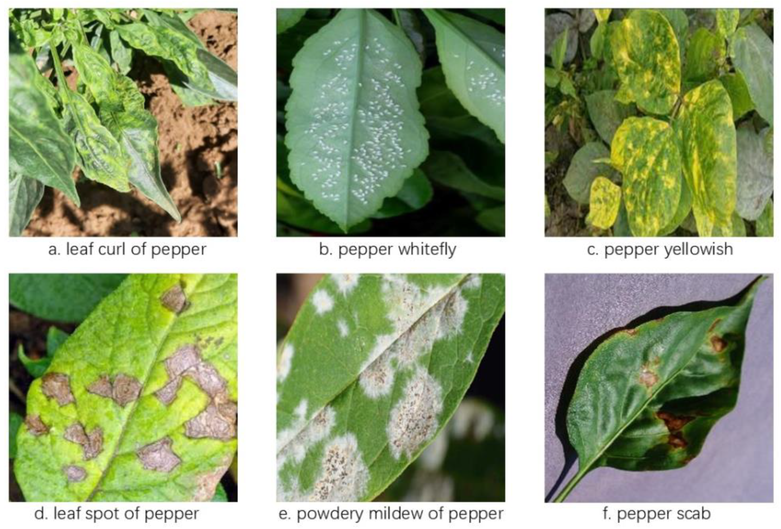
Figure 2.
Graphical representation of data processing methods.
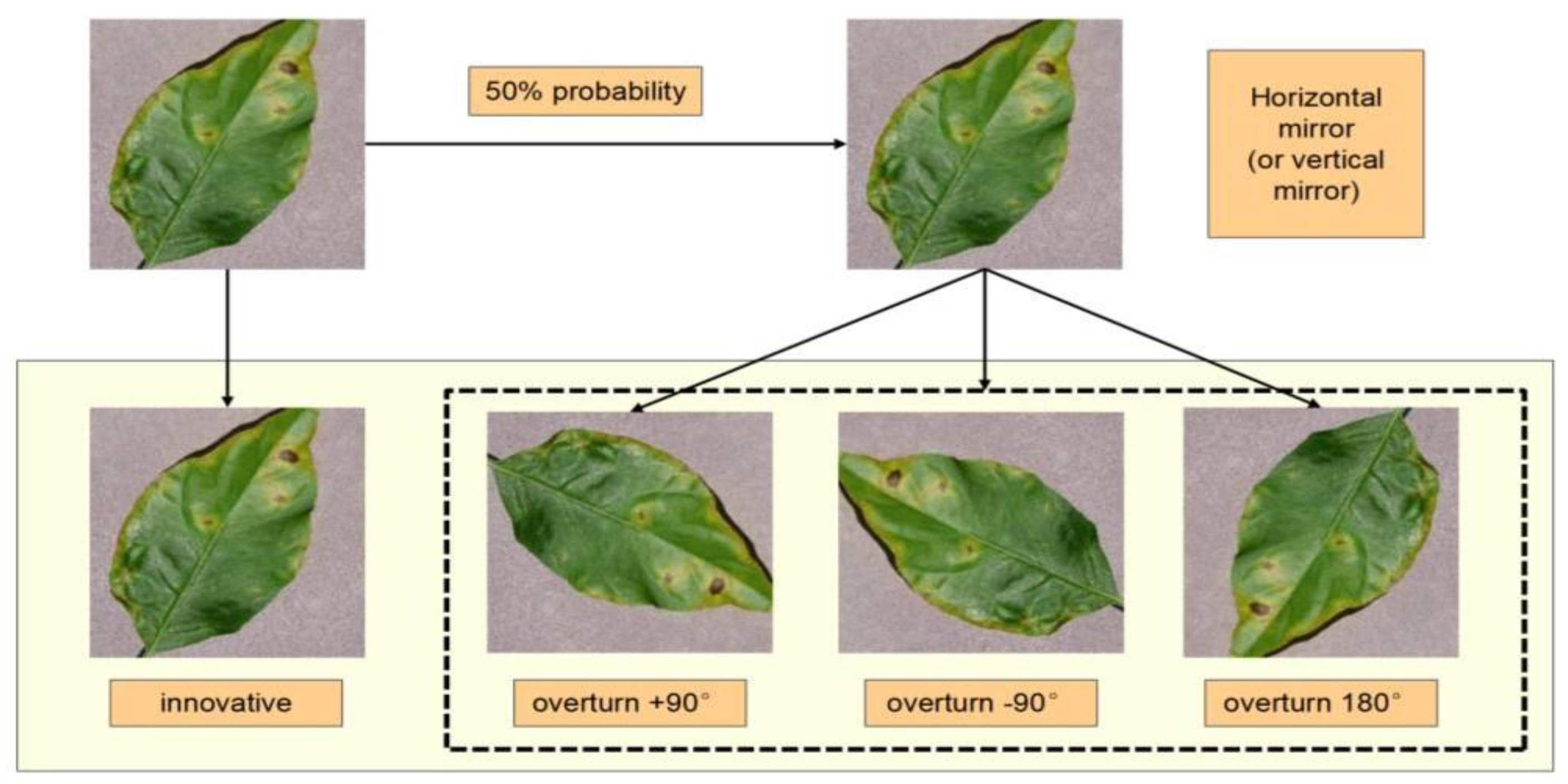
Figure 3.
DD-YOLO model diagram. Note: Conv is convolution; Concat is the feature connection module; DySample is the ultra-lightweight dynamic upsampler; SPPF_lSKA is the spatial pyramid pooling module that introduces the LSKA attention mechanism; C2f_iRBM and C2f_DCNv2 are both the C2f modules with partial convolution added to them; Detect is the detection head; Bbox.Loss and Cls. Cls.Loss are the bounding box loss and classification loss functions, respectively; p3, p4 and p5 are the small, medium and large feature map sizes, respectively.
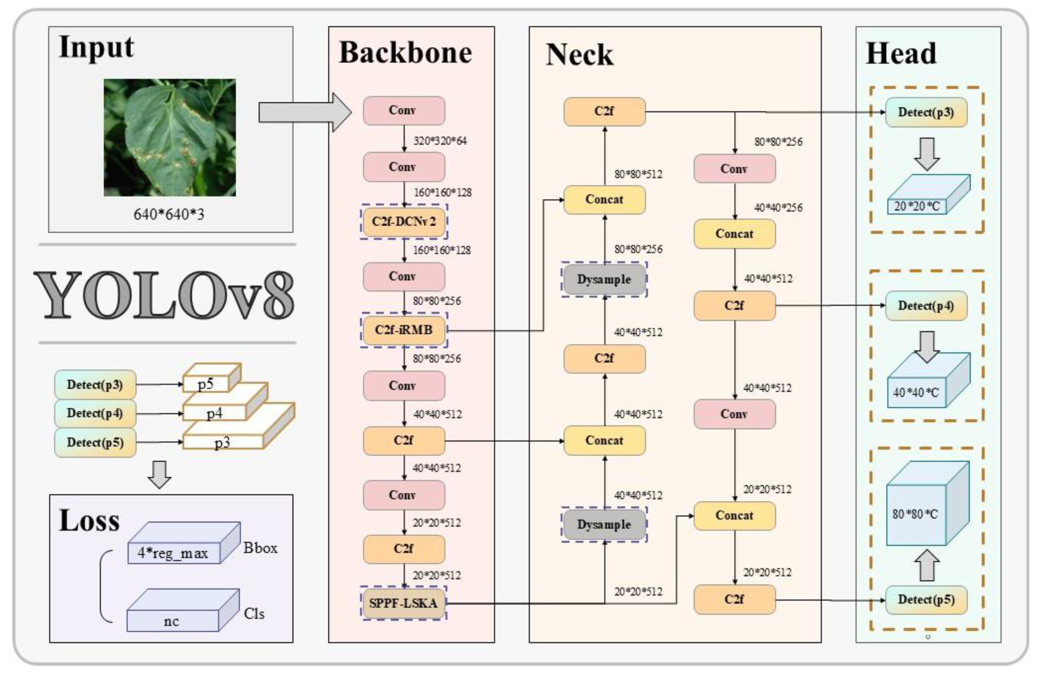
Figure 4.
iRMB structural paradigm. Note: DW-Conv is Deep Separable Convolutional Neural Network; Attn Mat is Attention Mechanism Matrix; Q is Query; K is Key; V is Value
Figure 4.
iRMB structural paradigm. Note: DW-Conv is Deep Separable Convolutional Neural Network; Attn Mat is Attention Mechanism Matrix; Q is Query; K is Key; V is Value
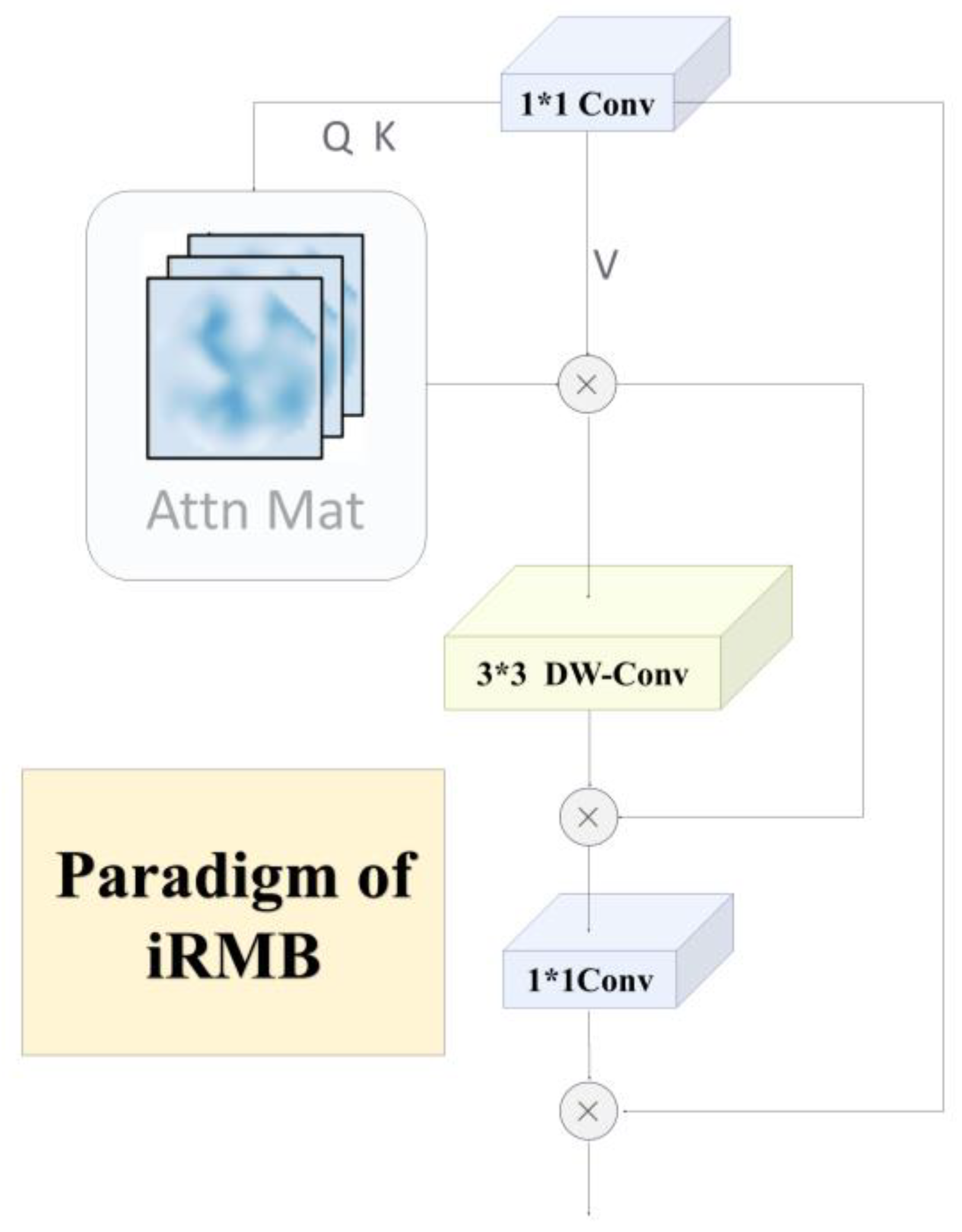
Figure 5.
Schematic diagram of DCNv2 structure. Note: h is the output of the hidden layer; x is the output or intermediate data of different layers in the network. The convolution operation of DCNv2 can be expressed as
Figure 5.
Schematic diagram of DCNv2 structure. Note: h is the output of the hidden layer; x is the output or intermediate data of different layers in the network. The convolution operation of DCNv2 can be expressed as
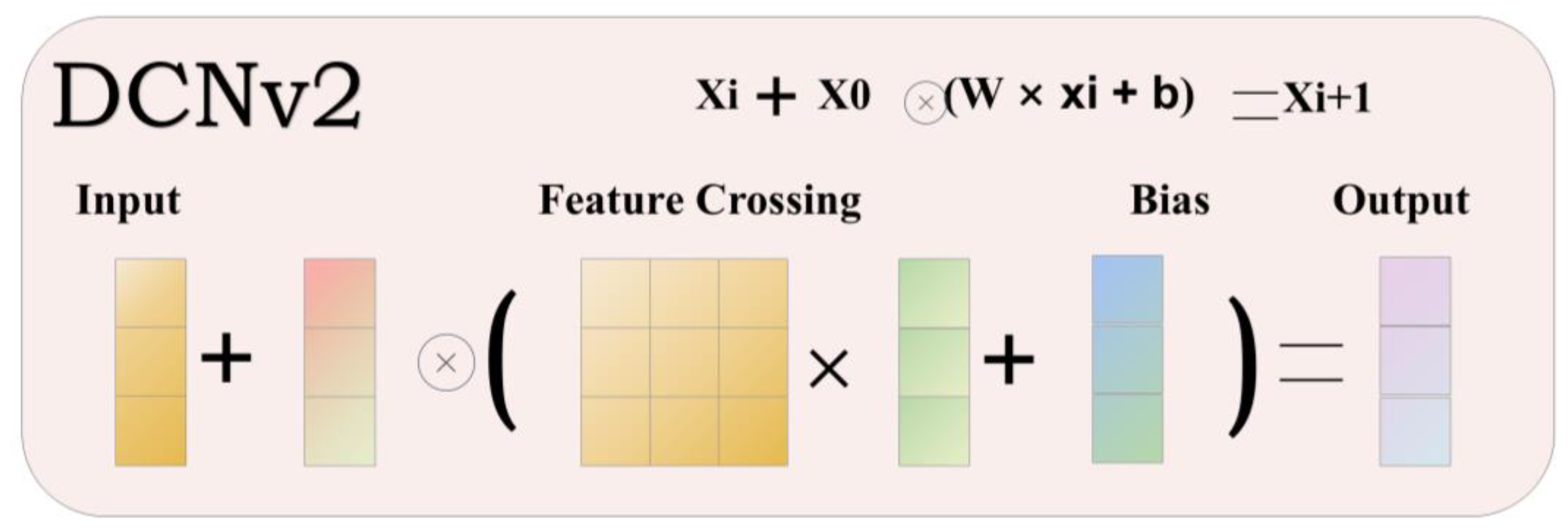
Figure 6.
DySample structure. Note: C is the number of channels of the input feature map; H is the height of the feature map; W is the width of the feature map; pixel shuffle is the image super-resolution reconstruction. (a) The sampling set is generated by a sample point generator that resamples the input features via a grid sampling function.
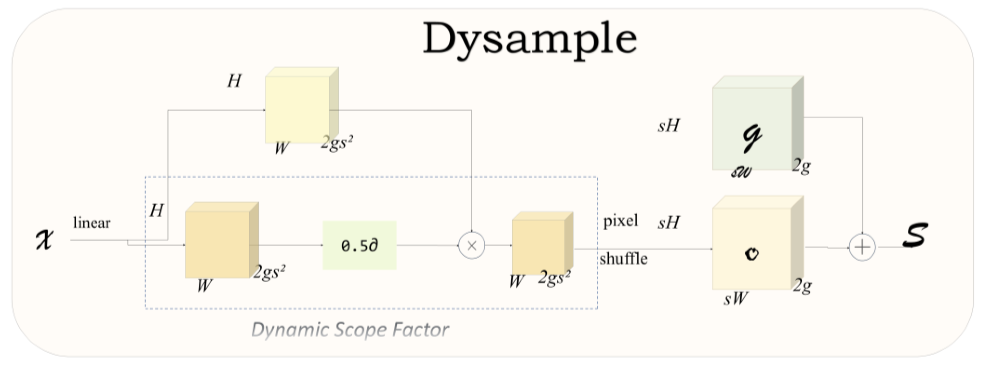
Figure 7.
Schematic diagram of LSKA structure. Note: Max-Pool2d is maximum pooling; both DW-D-Conv and DW-Conv are depth separable convolutional neural networks.
Figure 7.
Schematic diagram of LSKA structure. Note: Max-Pool2d is maximum pooling; both DW-D-Conv and DW-Conv are depth separable convolutional neural networks.
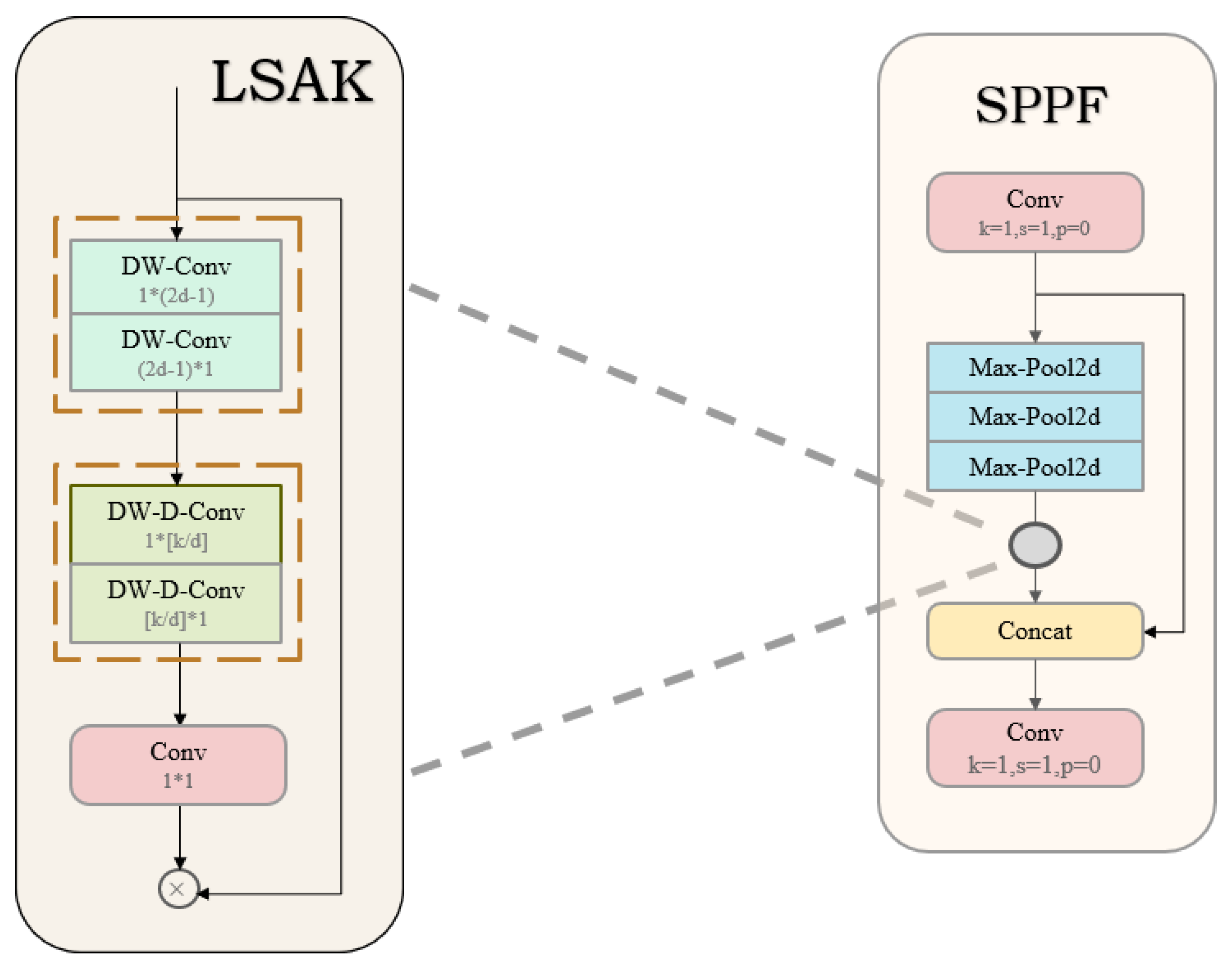
Figure 8.
Comparison of model feature visualization.
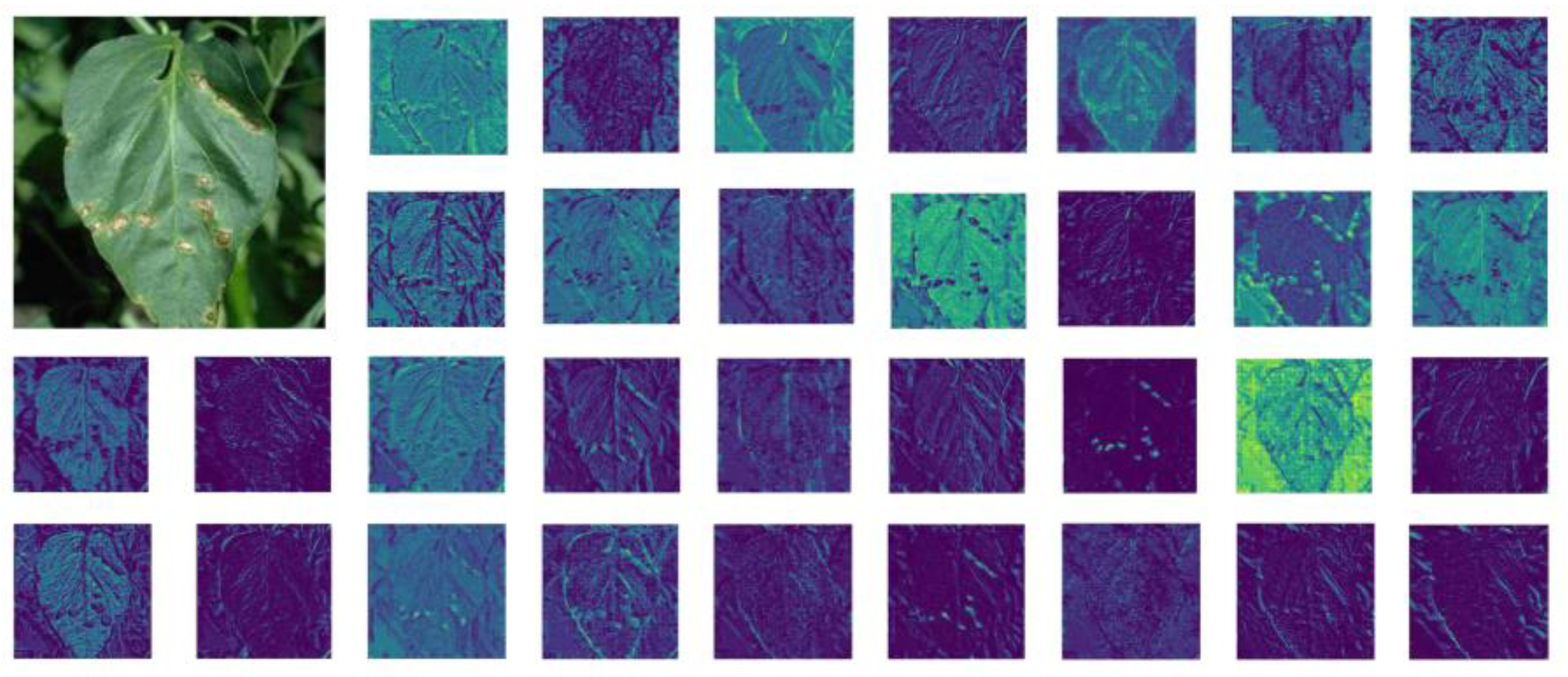
Figure 9.
Comparison of model heat map visualization.
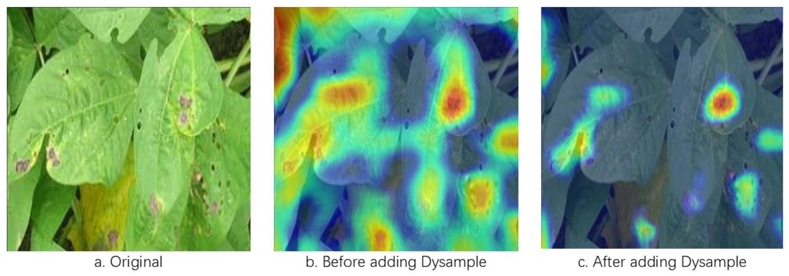
Figure 10.
Detection Comparison.
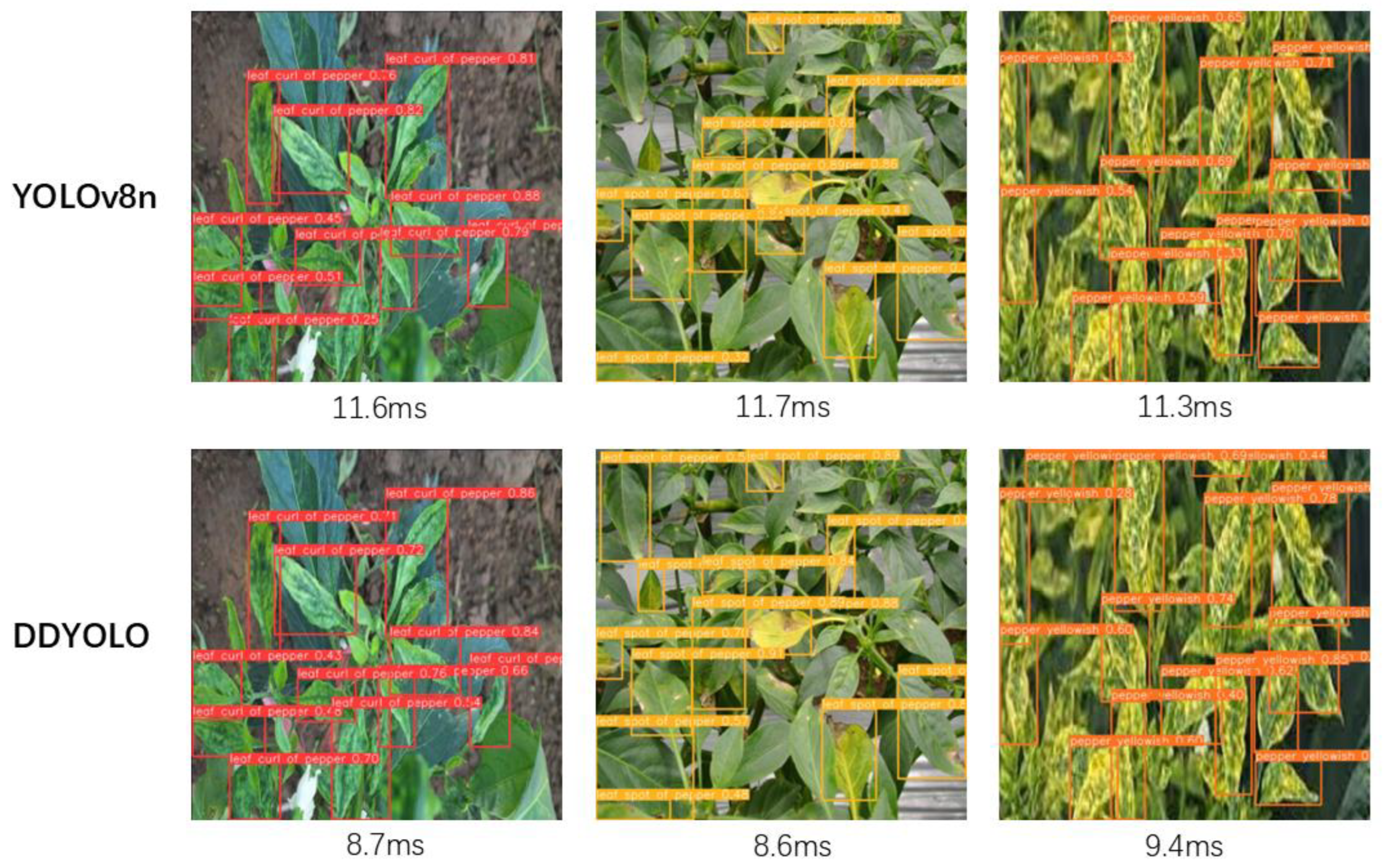

Table 1.
Distribution of chili pepper dataset.
| Class | Train | Val | All | Labels |
|---|---|---|---|---|
| leaf curl of pepper | 438 | 49 | 487 | 3498 |
| pepper whitefly | 311 | 34 | 345 | 482 |
| pepper yellowish | 365 | 41 | 406 | 3402 |
| leaf spot of pepper | 444 | 49 | 493 | 1155 |
| powdery mildew of pepper | 258 | 29 | 287 | 467 |
| pepper scab | 85 | 9 | 94 | 94 |
Table 2.
Server configuration.
| mirroring | PyTorch 1.11.0 Python 3.8 (ubuntu20.04) Cuda 11.3 |
|---|---|
| GPU | RTX 2080 Ti (11GB)*1 |
| CPU | 12 vCPU Intel(R) Xeon(R) Platinum 8255C CPU @ 2.50GHz |
Table 3.
Comparison of different lightweight feature extraction backbone networks.
| Backbone network | P/% | R/% | mAP/% | GFLOPs |
|---|---|---|---|---|
| C2f-iRMB | 87.5 | 85.0 | 90.8 | 7.0 |
| HGNetV2 | 80.3 | 76.2 | 82.7 | 6.9 |
| chostHGNetV2 | 78.9 | 75.1 | 81.5 | 6.8 |
| RepHGNetV2 | 79.9 | 75.5 | 82.9 | 6.9 |
| C2f-AKConv | 83.5 | 79.5 | 85.9 | 7.2 |
| C2f-MSBlock | 81.7 | 77.0 | 84.0 | 7.7 |
Table 4.
Ablation experiments.
| Test No. | Base model | DCNV2 | iRMB | DySample | LSKA | Precision P/% | Recall R/% | mAP50/% | Weights/MB | parameters | GFLOPs |
|---|---|---|---|---|---|---|---|---|---|---|---|
| 1 | YOLOv8n | × | × | × | × | 85.4 | 86.6 | 91.6 | 6.2 | 3006818 | 8.1 |
| 2 | √ | × | × | × | 89.9 | 89.8 | 94.5 | 6.3 | 3038205 | 8.0 | |
| 3 | × | √ | × | × | 87.5 | 85.0 | 90.8 | 5.5 | 2634194 | 7.0 | |
| 4 | × | × | √ | × | 90.1 | 89.9 | 94.5 | 6.3 | 3019170 | 8.1 | |
| 5 | × | × | × | √ | 90.0 | 89.7 | 94.4 | 6.8 | 3279714 | 8.3 | |
| 6 | √ | √ | × | × | 88.9 | 86.7 | 92.6 | 6.0 | 2893549 | 7.1 | |
| 7 | × | √ | √ | × | 88.4 | 84.7 | 91.0 | 5.5 | 2646546 | 7.1 | |
| 8 | × | × | √ | √ | 90.0 | 89.8 | 94.3 | 6.8 | 3292066 | 8.3 | |
| 9 | √ | × | √ | × | 90.1 | 89.1 | 94.3 | 6.3 | 3050557 | 8.0 | |
| 10 | √ | × | × | √ | 91.3 | 89.7 | 94.5 | 6.8 | 3311101 | 8.2 | |
| 11 | × | √ | × | √ | 86.9 | 84.6 | 90.4 | 6.1 | 2907090 | 7.3 | |
| 12 | √ | √ | √ | × | 88.0 | 87.2 | 92.0 | 6.0 | 2905901 | 7.1 | |
| 13 | × | √ | √ | √ | 88.1 | 83.7 | 90.6 | 6.1 | 2919442 | 7.3 | |
| 14 | √ | × | √ | √ | 90.4 | 88.9 | 94.3 | 6.9 | 3323453 | 8.2 | |
| 15 | √ | √ | × | √ | 87.9 | 85.8 | 91.4 | 6.6 | 3166445 | 7.3 | |
| 16 | √ | √ | √ | √ | 91.6 | 88.9 | 94.4 | 4.8 | 2296804 | 7.2 |
Note: √ indicates that the algorithm is used; × indicates that the algorithm is not used.
Table 5.
Comparison of different models of pepper disease detection results.
| Models | Precision % |
Recall % |
mAP@0.5 % |
mAP@0.5~0.95 % |
|---|---|---|---|---|
| SSD | 85.7 | 78.8 | 84.6 | 81.5 |
| Faster-RCNN | 60.1 | 92.4 | 86.8 | 71.8 |
| YOLOv5n | 62.7 | 68.9 | 70.3 | 39.6 |
| YOLOv8n | 85.4 | 86.6 | 91.6 | 68.7 |
| DD-YOLO | 91.6 | 88.9 | 94.4 | 72.6 |
Table 6.
The loss function of the GAN model and the probability of its generation.
| Model | Loss_D | Loss_G | D(x) | D(G(z)) |
|---|---|---|---|---|
| GAN | 0.0004~4.6782 | 2.74~28.27 | 0.78~1.00 | 0.0000~0.0948 |
Disclaimer/Publisher’s Note: The statements, opinions and data contained in all publications are solely those of the individual author(s) and contributor(s) and not of MDPI and/or the editor(s). MDPI and/or the editor(s) disclaim responsibility for any injury to people or property resulting from any ideas, methods, instructions or products referred to in the content. |
© 2025 by the authors. Licensee MDPI, Basel, Switzerland. This article is an open access article distributed under the terms and conditions of the Creative Commons Attribution (CC BY) license (http://creativecommons.org/licenses/by/4.0/).
Copyright: This open access article is published under a Creative Commons CC BY 4.0 license, which permit the free download, distribution, and reuse, provided that the author and preprint are cited in any reuse.


