Submitted:
24 October 2024
Posted:
24 October 2024
You are already at the latest version
Abstract
Breathing in fine particulate matter with diameters less than 2.5 µm (PM2.5) has greatly increased an individual’s risk of cardiovascular and respiratory diseases. As climate change progresses, extreme weather events, including wildfires, are expected to rise, exacerbating air pollution. The 2023 Canadian wildfires highlighted the growing threat of PM2.5 as smoke spread across U.S. cities like New York, Philadelphia, and Washington D.C. This research investigates the application of data augmentation techniques to improve the accuracy of PM2.5 concentration forecasts in these urban environments. Models trained on imbalanced datasets often struggle to capture extreme pollution events, underestimating high PM2.5 levels due to the model’s focus on more frequent, low-value samples. To address this, we implemented cluster-based undersampling and trained transformer models using various cutoff thresholds (12.1 µg/m³ and 35.5 µg/m³) and partial sampling ratios (10/90, 20/80, 30/70, 40/60, 50/50). Our results demonstrate that the 35.5 µg/m³ threshold, coupled with a 20/80 partial sampling ratio, provides the best performance regarding RMSE and R², particularly in capturing high PM2.5 events. Overall, models trained on augmented data significantly outperformed those trained on original data, highlighting the importance of resampling techniques in improving air quality forecasting accuracy, especially for high-pollution scenarios. These insights significantly contribute to a better understanding of PM2.5 pollution with the hopes of more informed public health and environmental policies.
Keywords:
Air Quality
; PM2.5 Forecasting
; Data Augmentation
; Cluster-Based Under Sampling
; Transformer Model
; 2023 Canadian Wildfires
1. Introduction
Air pollution remains one of the most pressing global health challenges, identified as the second leading risk factor for premature death worldwide. In 2021 alone, air pollution was responsible for approximately 8.1 million deaths globally, underscoring its profound impact on human health (State of Global Air Report, 2024). Fine particulate matter (PM2.5) is particularly concerning, as it refers to particles with an aerodynamic diameter of 2.5 micrometers or less. PM2.5 particles are small enough to penetrate deep into the lungs and even enter the bloodstream, posing significant risks to human health. The Global Burden of Disease (GBD) study estimated that ambient PM2.5 exposure was responsible for approximately 4.14 million deaths globally in 2019 (McDuffie et al., 2021). These particles are associated with a wide range of health outcomes, including stroke, ischemic heart disease, chronic obstructive pulmonary disease (COPD), and lung cancer (Gao et al., 2021; Gilcrease et al., 2020; Hystad et al., 2020; Lao et al., 2019; L. Liu et al., 2021; Thangavel et al., 2022). The respiratory system, especially the lungs, is vulnerable to PM2.5-induced toxicity, leading to inflammation and impaired immune responses, increasing susceptibility to respiratory infections (Jia et al., 2021). Growing evidence suggests that PM2.5 exposure is also linked to neurodegenerative diseases. The small size of the particles enables them to penetrate the brain via the olfactory nerve (Lee et al., 2019). Recent trends have shown an alarming increase in PM2.5 emissions due to wildfires, exacerbated by climate change and land management practices. Wildfire-related PM2.5 pollution has been observed to travel long distances, affecting regions far beyond the initial fire location (Sharma et al., 2022). Wildfires in the western United States have increased in frequency and intensity since the mid-1980s, primarily driven by rising temperatures and earlier spring snowmelt (Westerling et al., 2006). Climate projections suggest that the area affected by wildfires in the western U.S. could expand by 54% between 2046 and 2055 compared to 1996-2005 (Spracklen et al., 2009). This increase is compounded by a century of fire suppression practices, which have contributed to a dangerous buildup of flammable material in forests, as well as human activities that have escalated fire ignition rates (Balch et al., 2017; Boisramé et al., 2022).
During severe wildfire events, PM2.5 levels can spike to hazardous levels, exceeding the Environmental Protection Agency’s (EPA) threshold of 225.5 μg/m³ for hazardous air quality (EPA AQI, 2024). Artificial Intelligence/Machine Learning (AI/ML) models have demonstrated strong performance in forecasting PM2.5 under lower concentrations, but their accuracy diminishes for high-value PM2.5 levels (Yan et al., 2021). Studies have consistently shown that PM2.5 concentrations are underestimated when they exceed 60 μg/m³, particularly during severe pollution events (T. Li et al., 2017; J. Liu et al., 2022). These extreme events lead to a data imbalance, as high PM2.5 levels are underrepresented during training, making it difficult for models to predict these rare but critical conditions accurately (Z. Ma et al., 2014; Xu et al., 2018; Zhan et al., 2017). Although this challenge is well-known, relatively few studies have focused on solutions for improving predictions of extreme PM2.5 levels (Lu et al., 2021; Xiao et al., 2021; S. Zhang et al., 2022). Data augmentation techniques have addressed imbalanced data problems in ML, particularly in remote sensing applications (Feng et al., 2019a; Stivaktakis et al., 2019; X. Yu et al., 2017). Oversampling techniques, such as the Synthetic Minority Oversampling Technique (SMOTE) and Adaptive Synthetic Sampling (ADASYN), have been applied across various domains to mitigate the effects of imbalanced datasets (Khan et al., 2024). Conversely, under-sampling techniques like random under-sampling and more advanced methods, including cluster-based under-sampling using k-means, aim to reduce the dominance of majority classes while maintaining the dataset's representativeness (Lin et al., 2017; Yen & Lee, 2009). These strategies provide a foundation for enhancing model performance, particularly when dealing with extreme pollution values.
In recent years, transformer models, originally developed for Natural Language Processing (NLP), have shown promise for long-term air quality predictions due to their ability to capture long-range dependencies in time series data (Dong et al., 2024). Unlike recurrent models, transformers rely on self-attention mechanisms that allow more efficient information flow across sequences (Vaswani et al., 2017). These models have already demonstrated superior performance in fields such as machine translation (Neishi & Yoshinaga, 2019; Vaswani et al., 2017), speech recognition (X. Chen et al., 2020; Zeyer et al., 2019), and image segmentation (Bazi et al., 2021; Duke et al., 2021), indicating their potential for improving air quality forecasts, particularly in capturing complex, long-term pollutant behavior (Yue et al., 2020; Zhou et al., 2021).
Despite the advancements in data augmentation techniques and the adoption of transformer models, accurately forecasting extreme PM2.5 levels remains challenging. Current approaches often struggle with imbalanced datasets, where high PM2.5 concentrations are underrepresented, particularly during extreme pollution events like wildfire. This imbalance leads to poor model performance in forecasting. While some work has explored augmentation techniques like SMOTE and ADASYN (Flores et al., 2021; Yin et al., 2022), the specific application of these methods and advanced under-sampling techniques to PM2.5 forecasting during extreme events has been limited. Furthermore, the potential of transformer models to effectively forecast these events in urban environments remains underexplored, particularly in the context of data imbalance. To address these gaps, this research explores data augmentation techniques, specifically cluster-based undersampling with varying majority-to-minority class ratios and assesses its impact on high-value PM2.5 model performance. This study leverages a transformer model, which employs multi-head attention, to forecast PM2.5 concentrations in cases of extreme pollution events in urban areas such as New York City, Philadelphia, and Washington D.C. Additionally, the research investigates the impact of two EPA-defined minority-majority cutoff thresholds on model outcomes, highlighting the importance of robust models capable of accurately forecasting elevated PM2.5 levels in real-world scenarios. The specific research objectives are listed below:
- Augment imbalanced PM2.5 dataset with cluster-based undersampling with different combinations of majority-to-minority class ratios
- Investigate the impact of two minority-majority cutoff thresholds based on limits set by the EPA on model performance
- Build and train a transformer model to leverage the capabilities of multi-head attention in the context of PM2.5 forecasting
- Develop a robust forecasting model that accurately predicts PM2.5 concentrations, particularly during extreme pollution spikes caused by events like wildfires in New York City, Philadelphia, and Washington, D.C.
2. Literature Review
2.1. Data Augmentation Techniques for PM2.5
Data augmentation is a crucial tool in ML, particularly in situations where the dataset is imbalanced. By artificially increasing the diversity of the training set, data augmentation helps improve model robustness and generalization of modeling results (Feng et al., 2019; Z. Yang et al., 2023; Yin et al., 2022). Data augmentation techniques have already shown promise in many other fields, including air quality (Mi et al., 2024; Yin et al., 2022). Random oversampling (Moreo et al., 2016) and random undersampling (Mohammed et al., 2020) are simple methods to combat imbalanced datasets. Random oversampling randomly duplicates minority class samples. However, it often runs into problems of overfitting when used with conventional ML models (Mohammed et al., 2020). On the other hand, random undersampling randomly deletes the majority of observations, due to which it is prone to loss of information. Undersampling methods are often combined with clustering approaches. This involves initially clustering the data into several clusters using methods such as k-means clustering (Lin et al., 2017). The cluster-based undersampling method selects representative samples from each cluster to create a more balanced training dataset, ensuring a balanced representation of both classes (Yen & Lee, 2009). Other data augmentation techniques include SMOTE with k-means, the most prominent approach (Chawla et al., 2002). Although SMOTE was developed for classification problems, it can also be extended to regression problems (Torgo et al., 2013).
In the context of PM2.5 prediction, Yin et al. (2022) aimed to improve the estimation accuracy of high PM2.5 concentrations by using an AugResNet model with random oversampling and SMOTE. While their approach improved performance on high-value PM2.5 datasets, a limitation of the study was its focus on a single cutoff threshold and PM2.5 retrieval rather than forecasting, which limits its broader applicability. Flores et al. (2021) employed LSTM, GRU, and hybrid GRU+LSTM models with linear interpolation for data augmentation, expanding the dataset without addressing the imbalance between high and low PM2.5 concentrations. Their approach did not specifically target data imbalance, focusing instead on general dataset expansion, which can lead to overfitting, as synthetically increasing the dataset size does not introduce new variability. Mi et al. (2024) tackled the dataset shift problem between urban and rural PM2.5 data, addressing differences in predictor variable density using multiple imputations by chained equations; however, this study focused on correcting biases caused by variable density disparities rather than general PM2.5 forecasting, which limits its relevance to broader PM2.5 prediction challenges.
2.2. Transformer-Based PM2.5 Prediction Models
Statistical methods have traditionally been employed to estimate observed data directly, with linear approaches such as AutoRegressive Moving Average (ARMA), AutoRegressive Integrated Moving Average (ARIMA), and AutoRegressive Distributed Lag (ARDL) models being commonly used (Abedi et al., 2020; Cekim, 2020; Graupe et al., 1975; Jian et al., 2012). These models rely on the assumption of linearity, which limits their ability to capture the more complex, nonlinear relationships often present in environmental data like air quality. Nonlinear ML methods have gained significant traction for air quality forecasting because they can capture complex relationships and interactions between variables. Methods such as Support Vector Regression (SVR), Artificial Neural Networks (ANN), Random Forest (RF), and XGBoost offer more robust alternatives to linear models (Agarwal et al., 2020; Arhami et al., 2013; Chu et al., 2021; Gariazzo et al., 2020; W. Yang et al., 2018). ANNs have been widely used for air quality forecasting (Ding et al., 2016; H. Liu & Zhang, 2021; Zhao et al., 2020). ANNs can capture intricate patterns in time series data, making them suitable for forecasting tasks that require understanding temporal dynamics and spatial dependencies. However, while ANNs have been extensively used, traditional shallow neural networks are often limited in their feature learning capability. These models struggle to extract deep, abstract features from large datasets, which can hinder their performance, especially when faced with complex and highly nonlinear data.
More recent advancements, particularly in deep learning models, have addressed the limitations of traditional approaches by enhancing the depth of networks and improving feature extraction (Hinton & Salakhutdinov, 2006; Lecun et al., 2015). Several applications of these deep learning models have emerged in air quality forecasting. For instance, Autoencoder (AE) models have been used for air quality prediction (X. Li et al., 2016), while Convolutional Neural Networks (CNN)-based image recognition techniques have been applied to estimate PM2.5 concentrations from images (Chakma et al., 2017). Graph-based Long Short-Term Memory (LSTM) models have been employed to predict PM2.5 levels because of their ability to model spatial dependencies in air quality data (Gao & Li, 2021). A more advanced approach is the spatiotemporal Convolutional LSTM Extended (C-LSTME) model, which combines CNNs and LSTMs to capture high-level spatiotemporal features, improving air quality forecasting by modeling both spatial and temporal dependencies in the data (Wen et al., 2019). Hybrid models, which combine techniques such as CNNs, Gradient Boosting Machines (GBM), Bi-directional LSTMs (BiLSTM), and transfer learning, have been increasingly explored to improve air quality prediction performance (Luo et al., 2020; J. Ma et al., 2019; Z. Zhang et al., 2021).
Despite the success of deep learning (DL) models, they face significant challenges. Recurrent Neural Networks (RNNs) and LSTM networks suffer from gradient vanishing and exploding problems, limiting their ability to capture long-term dependencies. While useful for spatial learning, CNNs struggle to model complex, long-term relationships in time series datalike PM2.5. Transformer models, originally designed for NLP (Vaswani et al., 2017), have emerged as promising alternatives for addressing these limitations in air quality forecasting (Z. Zhang et al., 2021). For example, Zhou et al. (2021) introduced the Informer model, which improves temporal embeddings to learn non-stationary and long-range temporal dependencies. However, it focuses solely on "temporal attention" and overlooks spatial relationships between variables. Y. Li & Moura (2020) tackled this by developing a graph transformer that captures dynamic spatial dependencies, using sparse attention to trim less relevant nodes. Grigsby et al. (2021) further advanced this with the Spacetimeformer, which flattens multivariate time series to handle spatial and temporal influences. Recent models like the Sparse Attention-based Transformer (STN) by Z. Zhang & Zhang (2023) effectively reduce time complexity while capturing long-term dependencies in PM2.5 data. Similarly, M. Yu et al. (2023) proposed the SpatioTemporal (ST)-Transformer, designed to improve spatiotemporal predictions of PM2.5 concentrations in wildfire-prone areas.
The current research on PM2.5 forecasting reveals significant gaps, particularly in handling imbalanced datasets and modeling long-term dependencies. One of the main challenges is the underrepresentation of high PM2.5 concentration events, which are far less common than low concentrations. Traditional data augmentation techniques like random oversampling and undersampling have limitations such as overfitting and information loss, as highlighted by Mohammed et al. (2020). Although SMOTE provides an alternative by generating synthetic samples, its effectiveness in PM2.5 forecasting has been inconsistent, with studies like Yin et al. (2022) reporting higher RMSE compared to random oversampling. Additionally, models like RNNs and LSTMs, which are commonly used for PM2.5 forecasting, struggle with vanishing gradient problems and difficulties in capturing long-term dependencies, as noted by Wen et al. (2019). Recent advancements in Transformer models (Vaswani et al., 2017) offer a potential solution, as these models can capture long-range temporal dependencies through attention mechanisms. However, the application of Transformer models to wildfire-related PM2.5 forecasting remains underexplored, particularly in urban environments where pollution has severe health implications. The 2023 Canadian wildfires, which led to unprecedented PM2.5 levels in northeastern U.S. cities, provide an ideal dataset for addressing this gap. This study addresses the above-mentioned gaps by combining optimized resampling ratios and cluster-based undersampling to achieve a balanced representation of both high and low-concentration events (Lin et al., 2017). Furthermore, leveraging recent advancements like Informer and Spacetimeformer, the study introduces a Transformer-based architecture incorporating multi-head sparse attention to reduce time complexity while effectively learning complex temporal and spatial patterns. This research not only aims to address the issue of imbalanced datasets but also contributes to understanding wildfire-related PM2.5 spikes in urban centers such as New York City, Philadelphia, and Washington D.C., providing insights into the effectiveness of these models for real-time air quality predictions during extreme events.
3. Data
3.1. Study Area
The study focuses on major urban areas in the northeastern United States, specifically New York City, Philadelphia, and Washington, D.C. Figure 1 depicts the locations of AirNow sensors in three areas: New York City (11 stations), Philadelphia (5 stations), and Washington, D.C. (4 stations). The area, population, and geographical locations of these three cities are listed in Table 1. These cities are characterized by high population densities, significant traffic volumes, and industrial activities, all of which contribute to elevated levels of air pollution. Urban areas are often hotspots for PM2.5 due to vehicle emissions, industrial processes, and residential heating, making them critical regions for air quality monitoring and forecasting (Kloog et al., 2014; Qin et al., 2006). These urban environments also present challenges for air quality forecasting due to the complex interplay between local emissions and regional atmospheric transport processes.
A significant event that affected air quality in 2023 was the Canadian wildfires, which profoundly impacted pollution levels across North America, particularly in urban areas of the northeastern United States (Wang et al., 2024; M. Yu et al., 2024). The wildfires, which burned large swathes of forested areas in Canada, generated vast amounts of smoke and particulate matter that were transported southward by atmospheric winds, leading to unprecedented spikes in PM2.5 concentrations in cities like New York, Philadelphia, and Washington, D.C. (Bella, 2023). During this event, air quality in these cities reached hazardous levels, reducing visibility severely and prompting public health warnings (Deegan, 2023). PM2.5 forecasting is critical in these urban areas because it helps predict and mitigate the health risks associated with high pollution levels, especially during extreme events like the 2023 Canadian wildfires. Accurate forecasting allows for timely public health warnings (Xu et al., 2017). Additionally, it enables air quality agencies, such as the EPA, to take appropriate actions to reduce exposure to harmful particulate matter and manage air quality effectively, particularly during significant pollution episodes like wildfires.
3.2. Data Description
Table 2 outlines the variables used for forecasting PM2.5 concentrations, with PM2.5 from AirNow serving as the target variable. The covariates include aerosol optical depth (AOD) from the Moderate Resolution Imaging Spectroradiometer (MODIS) Multi-Angle Implementation of Atmospheric Correction (MAIAC) algorithm and various meteorological variables such as boundary layer height, relative humidity, temperature at 2 meters, surface pressure, and speed, all sourced from the European Centre for Medium-Range Weather Forecasts (ECMWF) ERA5 dataset. Additionally, elevation data, sourced from the United States Geological Survey (USGS), was used as a geographical covariate.
3.2.1. Ground-Level PM2.5 Measurements
Ground-level hourly PM2.5 measurements were obtained from the EPA's AirNow program, which provides near-real-time air quality data, including PM2.5 concentrations. The AirNow data undergoes a rigorous quality control process before being made available to the public. We downloaded PM2.5 data from AirNow sensors located in three major cities: New York City, Philadelphia, and Washington, D.C. through AirNow API (http://airnowapi.org). Given the need for timely analysis, we prioritized using near-real-time data over the delayed Air Quality System (AQS) data. These measurements were used to evaluate and compare model predictions of PM2.5 concentrations in the selected urban areas.
3.2.2. Satellite-Derived AOD
The AOD data used in this study was derived from the MODIS aboard the Terra and Aqua satellites, processed using the MAIAC algorithm. Terra and Aqua provide daily AOD products at a spatial resolution of 1 km × 1 km, captured at approximately 10:30 and 13:30 local time, respectively (Lyapustin et al., 2011, 2018). MAIAC is an advanced algorithm designed for aerosol retrievals over both dark vegetated surfaces and bright deserts, making it highly effective for air quality assessments due to its high spatial resolution (Liang et al., 2018; Z. Zhang et al., 2019). The Version 6 MAIAC Land AOD product has been widely applied in air quality studies due to its superior spatial resolution and temporal coverage (Lyapustin et al., 2018). For this study, we used the MAIAC AOD product MCD19A2 at 550 nm and retained only high-quality AOD values, as indicated by the quality assessment flag marked as "best quality". The data was sourced from the Level 1 and Atmosphere Archive and Distribution System Distributed Active Archive Center website (LAADS DAAC, 2024).
3.2.3. Meteorological Variables
Several studies have demonstrated the strong relationship between meteorological factors and variations in PM2.5 concentrations (Z. Chen et al., 2020; Huang et al., 2015). For this study, we utilized meteorological data from the ERA5 dataset, developed by the ECMWF. ERA5 is a comprehensive reanalysis product that estimates various atmospheric, land, and oceanic climate variables hourly. The dataset offers global coverage at a spatial resolution of 0.25° × 0.25° on a regular latitude-longitude grid (Dee et al., 2011; Hersbach et al., 2020). The data was sourced through the Copernicus Climate Data Store (C3S) in GRIB format, ensuring high detail and consistency for climate research. The meteorological variables selected for this study included boundary layer height (BLH), relative humidity, surface pressure (SP), 2-meter temperature (T2), and wind speed at 10 meters (U10/V10).
3.2.4. Geographical Variables
In this study, we used elevation data from the Global Multi-resolution Terrain Elevation Data 2010 (GMTED2010), which provides a spatial resolution of 30 arc-seconds (approximately 1 km). The data was obtained from the USGS website (GMTED2010, 2024).
4. Methodology
Figure 2 illustrates the workflow for the methodology used in this study to forecast PM2.5 levels. Starting with data acquisition, the data undergoes processing before selecting cutoff thresholds. Two cutoff thresholds are employed: 12.1 µg/m³ and 35.5 µg/m³, followed by applying various partial sampling ratios ranging from 10/90 to 50/50. Each threshold and sampling ratio combination is fed into a transformer model for model training. The accuracy of each model is assessed, and the best-performing model is selected to produce PM2.5 forecasts. This process allows for identifying the most effective threshold and sampling ratio, optimizing model performance for PM2.5 prediction.
4.1. Data Preprocessing and Collocation
We used the min-max scaler method to linearly transform the raw data to a value between 0 and 1 to balance the data dimensions and, at the same time, speed up the model to find the global optimal hyperparameters. The formula is as follows:
where and refer to the values before and after normalization, and min(x) and max(x) refer to the minimum and maximum values before normalization.
The data used in this study were aligned with the MAIAC AOD data for spatial and temporal matching. Meteorological variables from the ERA5 ECMWF and the AirNow PM2.5 datasets were matched to the Terra and Aqua MODIS satellite overpass times, which occur daily at approximately 10:30 and 13:30 local time. Daily averages of the hourly data were calculated within the overpass windows to ensure consistency. All variables were subsequently reprojected to the USA Contiguous Lambert Conformal Conic projection and resampled to a 1 km × 1 km resolution to ensure seamless integration with the MAIAC AOD data.
4.2. Cutoff Threshold
In their study, Yin et al. (2022) defined 75 µg/m³ as the cutoff threshold to distinguish low-value from high-value PM2.5 samples, aligning with China’s air quality standard, which classifies 75 µg/m³ as the lower limit for light PM2.5 pollution. The selection of a cutoff value for distinguishing between majority and minority classes plays a crucial role in determining class distribution and, consequently, the model’s performance in forecasting high-pollution periods. In the context of air quality in the United States, we used PM2.5 classifications by the EPA to determine cutoff threshold values (EPA AQI, 2024). To evaluate the sensitivity of model performance to different cutoff values, this study compares two thresholds aligned with EPA standards: 12.1 µg/m³ and 35.5 µg/m³.
The total dataset in this study consisted of 4,026,240 valid samples. With a cutoff threshold of 12.1 µg/m³, 3,472,689 samples were classified as “low-value,” and 553,551 samples were classified as “high-value.” The ratio of high-value samples to low-value ones was approximately 4:25 in the whole dataset. Ratios by city and the specific number of low- and high-value samples are listed in Table 3.
With a cutoff threshold of 35.5 µg/m³, 4,004,433 samples were classified as “low-value”, and 21,807 samples were classified as “high-value.” The ratio of high-value samples to low-value ones was approximately 5:1000 in the whole dataset. Ratios by city are listed in Table 4 and the specific number of low and high-value samples.
4.3. Cluster-Based Undersampling
In this study, we implemented cluster-based undersampling to address class imbalance in the training data. The first step involved grouping data points into clusters using the k-means algorithm, which organized the data based on feature similarities. This clustering approach preserved the inherent structure of the dataset by ensuring that similar data points were grouped together, which is crucial for maintaining data integrity when performing undersampling. By applying the undersampling strategy within each cluster, we selected a subset of instances, effectively reducing the majority class without losing the diversity within the data. This method allowed for a more representative sample, ensuring that both majority and minority classes were evenly distributed.
Before applying data augmentation, 20% of the original dataset was set aside for testing. The remaining 80% was used for model training, with samples drawn randomly based on the data augmentation technique. This approach ensured that each model was trained on datasets with unique sampling strategies, but all models were evaluated against a consistent testing dataset. The testing dataset was intentionally designed to mirror the original data distribution, ensuring fair comparisons across models trained on different augmented datasets.
Many studies aim to achieve a perfect 50/50 balance between minority and majority class samples. However, this idealized ratio is not always the most effective for model training, especially when dealing with environmental data like PM2.5, where the natural distribution is often skewed. Partial sampling, as discussed by Kamalov et al. (2022), involves adjusting the class ratio to values between the original class distribution and an equal 50/50 split. This technique provides a more nuanced approach, reflecting real-world distributions more accurately while improving model generalizability.
Kamalov et al. (2022) found that a minority-to-majority class ratio of approximately 0.75 was optimal in many scenarios, based on a systematic review of datasets and resampling techniques. Following this insight, the present study applied various partial sampling ratios to explore whether these findings hold for PM2.5 forecasting models. The aim was to determine whether a similar class balance could yield improved prediction accuracy in this context.
Initially, the training dataset contained around 3 million samples. However, after data augmentation and resampling, each training dataset was reduced to approximately 35,000 samples. Although all training datasets had the same number of observations, the distribution of PM2.5 values varied according to the selected threshold and resampling ratio, reflecting the impact of these parameters on the dataset’s composition. Table 5 shows the exact number of high-value and low-value samples for each partial sampling ratio dataset. Although the two cutoff thresholds result in the same number of high-value and low-value samples at each partial sampling ratio, their classification of high and low values differ, leading to distinct distributions across the datasets.
Figure 3 presents the distributions of training datasets across partial sampling ratios using a 12.1 µg/m³ threshold, with different partial sampling ratios of 10/90, 20/80, 30/70, 40/60, and 50/50. These sampling ratios represent the proportion of minority (high PM2.5) to majority (low PM2.5) samples included in the dataset.
The graphs in Figure 4 present the distributions of training datasets across partial sampling ratios using a 35.5 µg/m³ threshold, with different partial sampling ratios of 10/90, 20/80, 30/70, 40/60, and 50/50.
4.4. Transformer Model Architecture
The Transformer model has revolutionized various domains of ML, including NLP and time series forecasting (Vaswani et al., 2017). In the context of PM2.5 forecasting, the Transformer model's ability to capture long-range dependencies and complex temporal patterns makes it a powerful tool for forecasting air pollution levels (Cui et al, Zhang and Zhang). Traditional methods often struggle with the non-linear and dynamic nature of PM2.5 data, but the Transformer's self-attention mechanism allows it to weigh the importance of different time steps effectively, leading to more accurate and robust forecasts.
4.4.1. Positional Encoding
A Transformer model differentiates itself from traditional convolutional and recurrent neural networks by employing a novel positional encoding mechanism to preserve temporal relationships. This is achieved by embedding sine and cosine functions of varying frequencies into the normalized input sequences as illustrated by the formulas below:
Here, pos represents the position of a data point within the sliding window, and i indicates the i-th dimension in the feature space. This approach allows the Transformer to retain the order of the sequence data, ensuring that the temporal dynamics are preserved and effectively leveraged during training and inference (Vaswani et al. 2017).
4.4.2. Multi-Head Attention
To make the model focus on assigning different weights to the input time series information during the encoding phase, an attention mechanism is often used to quantify the dependencies between them. The attention score determines the extent to which the information corresponding to a time slice in the time series should be focused on in future forecasts, and it can be calculated using the scaled dot-product of the attention function as follows:
where Q, K, and V are the matrices of the queries, keys, and values, respectively, and dk is the dimension of the key (K). The input sequence is downsampled using the embedding layers to obtain (a1, a2, a3, …, at), which is multiplied by the learned matrices WQ, WK, and WV to obtain qi, ki and vi, i ∈ (1, 2, 3, …, t).
The multi-head attention mechanism enhances the model's ability to capture long-range dependencies by allowing it to focus on both sequence positions and multiple heads simultaneously. Each pollution factor's position, feature, and value are treated as separate heads, with multiple matrices applied to repeat the self-attention process across parallel layers. This approach enables the model to consider various relationships between pollution factors and meteorological conditions.
4.4.3. Encoder
In this study, the encoder consists of a stack of N = 6 identical layers. In each layer, the input goes through multi-head self-attention, where the same input is used for queries, keys, and values, and attention weights are computed based on the provided mask. The output from self-attention is added to the original input, normalized using LayerNorm, and passed through a feed-forward network. After the feed-forward computation, the result is again added to the input, followed by another layer normalization and dropout.
4.4.4. Decoder
Each decoder also consists of a stack of N = 6 layers. In each decoder layer, the first step applies self-attention, where the target sequence attends to itself, with a mask to control the attention. Next, cross-attention is applied, where the output from the self-attention step attends to the encoder output, allowing the decoder to incorporate information from the encoder while applying a source mask. Finally, the result passes through a feed-forward network, and after each attention and feed-forward step, residual connections, normalization, and dropout are applied to maintain stability.
4.5. Model Training and Evaluation
4.5.1. Model Training and Hyperparameter Tuning
Before applying data augmentation, 20% of the dataset was reserved for testing. The remaining 80% was used to create training datasets. This allowed models to be trained on varied datasets while being tested on a consistent, representative test set for fair comparison. More detailed dataset creation procedures can be found in Section 4.3.
In our research, we opted not to perform extensive hyperparameter tuning given that the hyperparameters specified in our experiments, as outlined in Table 6, already yielded satisfactory results. The parameters used in this study were determined through trial and error, like the approach by Cui et al. (2023). It is also important to note that the original authors of the transformer did not perform extensive hyperparameter tuning, and many subsequent studies employing transformers have followed a similar approach due to the high computational expense of such tuning (Vaswani et al., 2017; Liu et al., 2019, Al-qaness et al. 2023, Yu et al. 2023, Cui et al. 2023, and Dai et al. 2024).
To maintain the validity of comparisons across different models and experiments, we kept the hyperparameters constant throughout all tests. This decision ensured that performance differences could be attributed to model adjustments rather than variations in tuning.
4.5.2. Accuracy Measures
This paper employs Root Mean Square Error (RMSE), mean absolute error (MAE), and the coefficient of determination (R²) as metrics for assessing model accuracy. RMSE evaluates the extent to which the predicted value curve aligns with the observed value curve. MAE measures the average absolute difference between the predicted and actual values. R² indicates the proportion of the variance in the dependent variable (y) that can be explained by the independent variable (x). The respective formulas for these calculations are as follows:
where n refers to the number of data, yi refers to the ith observed value, refers to the ith predicted value, refers to the average of all observed values.
5. Experiments and Results
5.1. Accuracy Assessment
For experiments performed with a cutoff threshold of 12.1µg/m³, accuracy metrics are displayed in Table 7. As the resampling ratio becomes more balanced, ranging from 10/90 to 50/50, both RMSE and MAE metrics generally decrease, indicating improved model performance. The best overall performance is observed at the 50/50 ratio, where the RMSE reaches 2.757, the MAE is 1.044, and R² achieves a value of 0.850. This R² value suggests that the 50/50 ratio offers the strongest correlation between forecasted and true PM2.5 values, making it the most effective configuration for balanced data.
Accuracy metrics for experiments performed with a cutoff threshold of 35.5 µg/m³ are shown in Table 8. Interestingly, the 20/80 resampling ratio emerges as the optimal configuration overall, achieving the lowest RMSE (2.080) and MAE (1.386), alongside the highest R² value of 0.914. This strong performance suggests that a 20/80 ratio balances the trade-off between capturing minority and majority samples while minimizing error. The same ratio also delivers the best results for high-value PM2.5 samples, with an RMSE of 15.353, MAE of 10.077, and an R² value of 0.778, demonstrating that it is particularly effective for extreme pollution levels.
When comparing the performance of models trained on the original dataset to those trained on resampled datasets, the original data consistently underperforms, particularly in terms of error metrics like RMSE and R². This pattern emphasizes the value of resampling techniques for improving model accuracy.
5.2. Partial Sampling Ratio
At a cutoff threshold of 12.1 µg/m³, in evaluating model performance across varying partial sampling ratios, both the full dataset and high-value sample tests demonstrate a clear trend: the 50/50 partial sampling ratio consistently yields optimal results, as displayed in Figure 6. For the full dataset, RMSE decreases as the sampling ratio becomes more balanced, reaching its lowest point at the 50/50 ratio. This indicates that more balanced data distribution significantly enhances forecast accuracy. Similarly, the R² value steadily increases, peaking at the 50/50 ratio, signaling the model's improved ability to capture long-range dependencies at this balanced ratio.
For high-value samples, the results further underscore the importance of balanced resampling. RMSE shows a marked decline, and MAE gradually reduces as the ratio approaches 50/50. The model's highest R² value at this point confirms its strongest performance in predicting high-value samples with greater accuracy. Overall, the 50/50 sampling ratio emerges as the optimal configuration, demonstrating that more evenly distributed data enhances the model's performance, particularly in forecasting high-value events.
Patterns of model performance across varying partial sampling ratios changes for the cutoff threshold of 35.5 µg/m³, as presented in Figure 7. For the whole dataset, RMSE decreases as the partial sampling ratio becomes more balanced, reaching its minimum at 20/80. However, as the ratio becomes more balanced at 30/70, 40/60, and 50/50, RMSE slightly increases, indicating that the most balanced ratios do not necessarily provide the best performance. In contrast, the R² value peaks at 20/80, demonstrating the model’s strongest correlation between forecasted and true values, but declines for more balanced ratios, suggesting that more even data distribution does not always improve model performance.
For high-value samples, RMSE shows a sharp decline from the original dataset, continuing to decrease at the 20/80 ratio, with further stabilization beyond this point. MAE follows a similar trend, with a steep drop at 20/80 and stabilization thereafter. This indicates that the 20/80 partial sampling ratio effectively minimizes errors for high-value samples. Similarly, R² improves significantly with more balanced resampling, reaching its peak at 20/80, and begins to drop afterward, highlighting that the model’s best correlation for high-value events is achieved at this ratio.
Overall, the 20/80 ratio provides the best performance across both the full dataset and high-value samples, delivering the lowest RMSE and highest R². The original dataset, without resampling, performs the worst in terms of RMSE and R², underscoring the value of resampling for improving forecast accuracy, particularly for high-value samples. Yin et al. (2022) also observed increasing RMSE with more balanced partial sampling ratios, although they reported decreasing RMSE with more balanced ratios, while we observed stabilizing RMSE and MAE beyond 20/80.
The discrepancy between RMSE and MAE in the original dataset arises from the nature of these metrics. RMSE amplifies the impact of large errors due to its squaring mechanism, making it highly sensitive to outliers, whereas MAE treats all errors equally, offering a more robust reflection of average performance. This suggests that the original dataset likely contains a few large outliers that inflate RMSE without significantly affecting MAE. As the partial sampling ratio becomes more balanced, the model improves at predicting high-value outliers (leading to lower RMSE), but loses some accuracy in predicting low-value events (causing a slight increase in MAE).
5.3. Cutoff Threshold
Models trained on the 35.5 µg/m³ threshold consistently outperformed those trained on the 12.1 µg/m³ threshold in terms of RMSE and R², as demonstrated in Figure 8. The resampling ratio plays a crucial role in model performance, with the 20/80 ratio emerging as optimal for the 35.5 µg/m³ threshold, while the 50/50 ratio works best for the 12.1 µg/m³ threshold. This disparity is largely driven by the nature of the data captured at each threshold. The higher 35.5 threshold likely includes a more concentrated set of high-value samples, making a less balanced ratio like 20/80 more effective since the distinct minority samples don’t require as much balancing. In contrast, the 12.1 threshold includes more low-value samples, necessitating a 50/50 ratio to adequately represent both minority and majority groups.
RMSE, which squares the differences before averaging, amplifies larger errors, making it more sensitive to a few large deviations from actual values. This explains why models trained on the 12.1 threshold performed worse in terms of RMSE, as the larger prediction errors had a greater impact. However, MAE, which treats all errors equally, performed better for the 12.1 threshold, indicating that while the errors were frequent, they were smaller in magnitude.
For the 35.5 µg/m³ threshold, RMSE decreases as the sampling ratio becomes more balanced, reducing large prediction errors, but eventually, as accuracy for low-value samples declines, RMSE starts to increase. Similarly, R² initially improves with more balanced ratios but reaches a peak at higher ratios, particularly for the 12.1 µg/m³ threshold. Beyond this point, additional balancing dilutes the model’s ability to capture key variance for low-value samples, leading to diminishing returns in overall accuracy.
5.4. Time Series Analysis
The one-day forecasts for PM2.5 from 2021-2023 in New York City, Philadelphia, and Washington D.C. produced by models trained on the original dataset show strong accuracy for lower PM2.5 concentrations, particularly for values below 30 µg/m³. This is reflected in the high similarity between forecasted and observed values at these low levels. However, the model struggles to predict higher PM2.5 concentrations, reaching a ceiling in magnitude when faced with extreme pollution events. This limitation arises from the imbalanced dataset, where the majority of samples consist of lower values, leading the model to prioritize these over the rarer high-value samples. As a result, the model is unable to fully capture extreme PM2.5 events, a challenge frequently highlighted in the literature, which shows that forecast accuracy tends to decline as PM2.5 levels increase.
In contrast, models trained on the augmented dataset, using a 35.5 µg/m³ cutoff threshold and a 40/60 partial sampling ratio, demonstrate improved performance in capturing high-value PM2.5 events. Although there is a trade-off, where the model's accuracy for lower PM2.5 levels is slightly reduced, this adjustment leads to significantly better RMSE and R-squared measures. This reflects the model’s enhanced ability to forecast more extreme pollution scenarios, a critical aspect in improving overall prediction accuracy for high PM2.5 concentrations. The trade-off is seen in the slightly worse MAE, as the augmented dataset introduces more diversity and some smaller errors that MAE treats equally, while RMSE emphasizes the larger improvements in extreme cases. The augmented model is better suited to handle high-value samples, which is particularly beneficial in scenarios where predicting extreme pollution is more critical than maintaining perfect accuracy at lower concentrations.
The key contrast between the two models lies in the distributional focus: the original dataset performs better on low-level PM2.5 concentrations but struggles with extreme values. In comparison, the augmented dataset sacrifices some accuracy at lower concentrations to better capture the high-value events, which are crucial for understanding and managing pollution spikes. This trade-off is especially visible in the improvements in terms of RMSE, which penalizes large errors more severely. These results show that the model trained on augmented data is significantly better at predicting higher PM2.5 values.
6. Discussion
The underestimation of high pollutant levels has been an issue frequently discussed in many studies (Li et al, 2017). This research addresses the challenge by applying data augmentation techniques prior to training the deep learning model. One of the key contributions of this study is the exploration of cluster-based undersampling, implemented at different cutoff thresholds and partial sampling ratios, which helped mitigate class imbalance and improve model performance. Our findings indicate that the higher cutoff threshold of 35.5 µg/m³ resulted in superior model performance when compared to the lower threshold of 12.1 µg/m³, as the 35.5 µg/m³ threshold more effectively differentiated between low- and high-value samples. The most optimal partial sampling ratio was found to be 20/80, consistent with Yin et al. (2022), which identified 30/70 as optimal in their study. Previous literature, including Kamalov et al. (2022), suggests that a fully balanced dataset is not always the best approach, and each dataset’s unique characteristics may necessitate different ratios. In our case, the 20/80 ratio paired with the 35.5 µg/m³ cutoff provided the best performance in capturing high-value samples without over-suppressing the majority class.
Future work could enhance the model by incorporating additional data sources that influence PM2.5 levels. Urban traffic data, which is crucial in accounting for emissions from vehicles, and industrial activity data from factories and power plants would provide more detailed insights into spikes in pollution. Including weather data such as wind patterns and forecasts could improve the model’s accuracy in predicting pollutant dispersion across regions. In addition to data augmentation through cluster-based undersampling, more advanced techniques like Generative Adversarial Networks (GANs) could be explored to generate realistic synthetic data for extreme pollution events, which are rare but critical to forecast. Expanding the model’s geographic scope by testing it on various cities would further strengthen its generalizability. Another promising avenue would be to extend the model to perform multistep predictions, forecasting PM2.5 concentrations over multiple time steps rather than just the next step, which would be particularly valuable for air quality forecasting over longer time periods like days or weeks. Moreover, broadening the scope of the model to predict other key pollutants such as NO2, SO2, and O3 would provide a comprehensive air quality forecasting system, enabling more effective city-level interventions to manage overall air quality.
7. Conclusion
This study demonstrates that the 35.5 µg/m³ threshold consistently outperforms the 12.1 µg/m³ threshold across key metrics like RMSE and R², likely due to its better representation of higher pollution values. The choice of partial sampling ratio proved crucial, with 50/50 optimal for the 12.1 threshold and 20/80 optimal for the 35.5 threshold, effectively balancing the need to capture both frequent and extreme pollution events. The model with the best performance (RMSE: 2.080, MAE: 1.386, R²: 0.914) utilized the 35.5 µg/m³ threshold and a 20/80 partial sampling ratio. Overall, models trained on resampled data significantly outperformed those trained on the original dataset, demonstrating the importance of data augmentation in handling imbalanced datasets and improving forecast accuracy, especially for high-value pollution scenarios. These findings highlight the critical role of threshold selection and resampling strategies in enhancing PM2.5 forecasting models.
References
- Abedi, A., Baygi, M. M., Poursafa, P., Mehrara, M., Amin, M. M., Hemami, F., & Zarean, M. (2020). Air pollution and hospitalization: an autoregressive distributed lag (ARDL) approach. Environmental Science and Pollution Research, 27(24), 30673–30680. [CrossRef]
- Agarwal, S., Sharma, S., R., S., Rahman, M. H., Vranckx, S., Maiheu, B., Blyth, L., Janssen, S., Gargava, P., Shukla, V. K., & Batra, S. (2020). Air quality forecasting using artificial neural networks with real time dynamic error correction in highly polluted regions. Science of The Total Environment, 735, 139454. [CrossRef]
- Arhami, M., Kamali, N., & Rajabi, M. M. (2013). Predicting hourly air pollutant levels using artificial neural networks coupled with uncertainty analysis by Monte Carlo simulations. Environmental Science and Pollution Research, 20(7), 4777–4789. [CrossRef]
- Balch, J. K., Bradley, B. A., Abatzoglou, J. T., Chelsea Nagy, R., Fusco, E. J., & Mahood, A. L. (2017). Human-started wildfires expand the fire niche across the United States. Proceedings of the National Academy of Sciences of the United States of America, 114(11), 2946–2951. [CrossRef]
- Bazi, Y., Bashmal, L., Al Rahhal, M. M., Dayil, R. Al, & Ajlan, N. Al. (2021). Vision Transformers for Remote Sensing Image Classification. Remote Sensing 2021, Vol. 13, Page 516, 13(3), 516. [CrossRef]
- Bella, T. (2023, June 8). Philadelphia’s hazardous air quality from Canadian wildfires is worst level in city since 1999 - The Washington Post. The Washington Post. https://www.washingtonpost.com/climate-environment/2023/06/08/philadelphia-air-quality-worst-wildfire-smoke/.
- Boisramé, G. F. S., Brown, T. J., & Bachelet, D. M. (2022). Trends in western USA fire fuels using historical data and modeling. Fire Ecology, 18(1), 1–34. [CrossRef]
- Cekim, H. O. (2020). Forecasting PM10 concentrations using time series models: a case of the most polluted cities in Turkey. Environmental Science and Pollution Research, 27(20), 25612–25624. [CrossRef]
- Chakma, A., Vizena, B., Cao, T., Lin, J., & Zhang, J. (2017). Image-based air quality analysis using deep convolutional neural network. Proceedings - International Conference on Image Processing, ICIP, 2017-September, 3949–3952. [CrossRef]
- Chawla, N. V., Bowyer, K. W., Hall, L. O., & Kegelmeyer, W. P. (2002). SMOTE: Synthetic Minority Over-sampling Technique. Journal of Artificial Intelligence Research, 16, 321–357. [CrossRef]
- Chen, X., Wu, Y., Wang, Z., Liu, S., & Li, J. (2020). Developing Real-time Streaming Transformer Transducer for Speech Recognition on Large-scale Dataset. ICASSP, IEEE International Conference on Acoustics, Speech and Signal Processing - Proceedings, 2021-June, 5904–5908. [CrossRef]
- Chen, Z., Chen, D., Zhao, C., Kwan, M. po, Cai, J., Zhuang, Y., Zhao, B., Wang, X., Chen, B., Yang, J., Li, R., He, B., Gao, B., Wang, K., & Xu, B. (2020). Influence of meteorological conditions on PM2.5 concentrations across China: A review of methodology and mechanism. Environment International, 139, 105558. [CrossRef]
- Chu, J., Dong, Y., Han, X., Xie, J., Xu, X., & Xie, G. (2021). Short-term prediction of urban PM2.5 based on a hybrid modified variational mode decomposition and support vector regression model. Environmental Science and Pollution Research, 28(1), 56–72. [CrossRef]
- Cui, B., Liu, M., Li, S., Jin, Z., Zeng, Y., & Lin, X. (2023). Deep learning methods for atmospheric PM2.5 prediction: A comparative study of transformer and CNN-LSTM-attention. Atmospheric Pollution Research, 14(9), 101833. [CrossRef]
- Dee, D. P., Uppala, S. M., Simmons, A. J., Berrisford, P., Poli, P., Kobayashi, S., Andrae, U., Balmaseda, M. A., Balsamo, G., Bauer, P., Bechtold, P., Beljaars, A. C. M., van de Berg, L., Bidlot, J., Bormann, N., Delsol, C., Dragani, R., Fuentes, M., Geer, A. J., … Vitart, F. (2011). The ERA-Interim reanalysis: configuration and performance of the data assimilation system. Quarterly Journal of the Royal Meteorological Society, 137(656), 553–597. [CrossRef]
- Deegan, D. (2023, June 7). Canadian Wildfires Prompt Poor Air Quality Alert for Parts of New England on June 7, 2023 US EPA. https://www.epa.gov/newsreleases/canadian-wildfires-prompt-poor-air-quality-alert-parts-new-england-june-7-2023.
- Ding, W., Zhang, J., & Leung, Y. (2016). Prediction of air pollutant concentration based on sparse response back-propagation training feedforward neural networks. Environmental Science and Pollution Research, 23(19), 19481–19494. [CrossRef]
- Dong, J., Zhang, Y., & Hu, J. (2024). Short-term air quality prediction based on EMD-transformer-BiLSTM. Scientific Reports 2024 14:1, 14(1), 1–17. [CrossRef]
- Duke, B., Ahmed, A., Wolf, C., Aarabi, P., & Taylor, G. W. (2021). SSTVOS: Sparse Spatiotemporal Transformers for Video Object Segmentation. Proceedings of the IEEE Computer Society Conference on Computer Vision and Pattern Recognition, 5908–5917. [CrossRef]
- EPA AQI. (2024). Final Updates to the Air Quality Index (AQI) for Particulate Matter - Fact Sheet and Common Questions.
- Feng, W., Boukir, S., & Huang, W. (2019). Margin-Based Random Forest for Imbalanced Land Cover Classification. International Geoscience and Remote Sensing Symposium (IGARSS), 3085–3088. [CrossRef]
- Flores, A., Valeriano-Zapana, J., Yana-Mamani, V., & Tito-Chura, H. (2021). PM2.5 prediction with Recurrent Neural Networks and Data Augmentation. 2021 IEEE Latin American Conference on Computational Intelligence, LA-CCI 2021. [CrossRef]
- Gao, X., Koutrakis, P., Coull, B., Lin, X., Vokonas, P., Schwartz, J., & Baccarelli, A. A. (2021). Short-term exposure to PM2.5 components and renal health: Findings from the Veterans Affairs Normative Aging Study. Journal of Hazardous Materials, 420, 126557. [CrossRef]
- Gao, X., & Li, W. (2021). A graph-based LSTM model for PM2.5 forecasting. Atmospheric Pollution Research, 12(9), 101150. [CrossRef]
- Gariazzo, C., Carlino, G., Silibello, C., Renzi, M., Finardi, S., Pepe, N., Radice, P., Forastiere, F., Michelozzi, P., Viegi, G., & Stafoggia, M. (2020). A multi-city air pollution population exposure study: Combined use of chemical-transport and random-Forest models with dynamic population data. Science of The Total Environment, 724, 138102. [CrossRef]
- Gilcrease, G. W., Padovan, D., Heffler, E., Peano, C., Massaglia, S., Roccatello, D., Radin, M., Cuadrado, M. J., & Sciascia, S. (2020). Is air pollution affecting the disease activity in patients with systemic lupus erythematosus? State of the art and a systematic literature review. European Journal of Rheumatology, 7(1), 31. [CrossRef]
- GMTED2010. (2024). USGS. https://www.usgs.gov/coastal-changes-and-impacts/gmted2010.
- Graupe, D., Krause, D. J., Moore, J. B., & Moore, J. B. (1975). Identification of Autoregressive Moving-Average Parameters of Time Series. IEEE Transactions on Automatic Control, 20(1), 104–107. [CrossRef]
- Grigsby, J., Wang, Z., Nguyen, N., & Qi, Y. (2021). Long-Range Transformers for Dynamic Spatiotemporal Forecasting. https://arxiv.org/abs/2109.12218v3.
- Hersbach, H., Bell, B., Berrisford, P., Hirahara, S., Horányi, A., Muñoz-Sabater, J., Nicolas, J., Peubey, C., Radu, R., Schepers, D., Simmons, A., Soci, C., Abdalla, S., Abellan, X., Balsamo, G., Bechtold, P., Biavati, G., Bidlot, J., Bonavita, M., … Thépaut, J. N. (2020). The ERA5 global reanalysis. Quarterly Journal of the Royal Meteorological Society, 146(730), 1999–2049. [CrossRef]
- Hinton, G. E., & Salakhutdinov, R. R. (2006). Reducing the dimensionality of data with neural networks. Science, 313(5786), 504–507. [CrossRef]
- Huang, F., Li, X., Wang, C., Xu, Q., Wang, W., Luo, Y., Tao, L., Gao, Q., Guo, J., Chen, S., Cao, K., Liu, L., Gao, N., Liu, X., Yang, K., Yan, A., & Guo, X. (2015). PM2.5 Spatiotemporal Variations and the Relationship with Meteorological Factors during 2013-2014 in Beijing, China. PLOS ONE, 10(11), e0141642. [CrossRef]
- Hystad, P., Larkin, A., Rangarajan, S., AlHabib, K. F., Avezum, Á., Calik, K. B. T., Chifamba, J., Dans, A., Diaz, R., du Plessis, J. L., Gupta, R., Iqbal, R., Khatib, R., Kelishadi, R., Lanas, F., Liu, Z., Lopez-Jaramillo, P., Nair, S., Poirier, P., … Brauer, M. (2020). Associations of outdoor fine particulate air pollution and cardiovascular disease in 157 436 individuals from 21 high-income, middle-income, and low-income countries (PURE): a prospective cohort study. The Lancet Planetary Health, 4(6), e235–e245. [CrossRef]
- Jia, H., Liu, Y., Guo, D., He, W., Zhao, L., & Xia, S. (2021). PM2.5-induced pulmonary inflammation via activating of the NLRP3/caspase-1 signaling pathway. Environmental Toxicology, 36(3), 298–307. [CrossRef]
- Jian, L., Zhao, Y., Zhu, Y. P., Zhang, M. B., & Bertolatti, D. (2012). An application of ARIMA model to predict submicron particle concentrations from meteorological factors at a busy roadside in Hangzhou, China. Science of The Total Environment, 426, 336–345. [CrossRef]
- Kamalov, F., Atiya, A. F., Elreedy, D. (2022). Partial Resampling of Imbalanced Data. [cs.LG] arXiv:2207.04631 [Preprint. [CrossRef]
- Khan, A. A., Chaudhari, O., & Chandra, R. (2024). A review of ensemble learning and data augmentation models for class imbalanced problems: Combination, implementation and evaluation. Expert Systems with Applications, 244, 122778. [CrossRef]
- Kloog, I., Chudnovsky, A. A., Just, A. C., Nordio, F., Koutrakis, P., Coull, B. A., Lyapustin, A., Wang, Y., & Schwartz, J. (2014). A new hybrid spatio-temporal model for estimating daily multi-year PM2.5 concentrations across northeastern USA using high resolution aerosol optical depth data. Atmospheric Environment, 95, 581–590. [CrossRef]
- LAADS DAAC. (2024). NASA. https://ladsweb.modaps.eosdis.nasa.gov/.
- Lao, X. Q., Guo, C., Chang, L. yun, Bo, Y., Zhang, Z., Chuang, Y. C., Jiang, W. K., Lin, C., Tam, T., Lau, A. K. H., Lin, C. Y., & Chan, T. C. (2019). Long-term exposure to ambient fine particulate matter (PM 2.5 ) and incident type 2 diabetes: a longitudinal cohort study. Diabetologia, 62(5), 759–769. [CrossRef]
- Lecun, Y., Bengio, Y., & Hinton, G. (2015). Deep learning. Nature 2015 521:7553, 521(7553), 436–444. [CrossRef]
- Lee, S., Lee, W., Kim, D., Kim, E., Myung, W., Kim, S. Y., & Kim, H. (2019). Short-term PM2.5 exposure and emergency hospital admissions for mental disease. Environmental Research, 171, 313–320. [CrossRef]
- Li, T., Shen, H., Yuan, Q., Zhang, X., & Zhang, L. (2017). Estimating Ground-Level PM2.5 by Fusing Satellite and Station Observations: A Geo-Intelligent Deep Learning Approach. Geophysical Research Letters, 44(23), 11,985-11,993. [CrossRef]
- Li, X., Peng, L., Hu, Y., Shao, J., & Chi, T. (2016). Deep learning architecture for air quality predictions. Environmental Science and Pollution Research, 23(22), 22408–22417. [CrossRef]
- Li, Y., & Moura, J. M. F. (2020). Forecaster: A Graph Transformer for Forecasting Spatial and Time-Dependent Data. Frontiers in Artificial Intelligence and Applications, 325, 1293–1300. [CrossRef]
- Liang, F., Xiao, Q., Wang, Y., Lyapustin, A., Li, G., Gu, D., Pan, X., & Liu, Y. (2018). MAIAC-based long-term spatiotemporal trends of PM2.5 in Beijing, China. The Science of the Total Environment, 616–617, 1589–1598. [CrossRef]
- Lin, W. C., Tsai, C. F., Hu, Y. H., & Jhang, J. S. (2017). Clustering-based undersampling in class-imbalanced data. Information Sciences, 409–410, 17–26. [CrossRef]
- Liu, H., & Zhang, X. (2021). AQI time series prediction based on a hybrid data decomposition and echo state networks. Environmental Science and Pollution Research, 28(37), 51160–51182. [CrossRef]
- Liu, J., Weng, F., & Li, Z. (2022). Ultrahigh-Resolution (250 m) Regional Surface PM2.5Concentrations Derived First from MODIS Measurements. IEEE Transactions on Geoscience and Remote Sensing, 60. [CrossRef]
- Liu, L., Zhang, Y., Yang, Z., Luo, S., & Zhang, Y. (2021). Long-term exposure to fine particulate constituents and cardiovascular diseases in Chinese adults. Journal of Hazardous Materials, 416, 126051. [CrossRef]
- Lu, Y., Giuliano, G., & Habre, R. (2021). Estimating hourly PM2.5 concentrations at the neighborhood scale using a low-cost air sensor network: A Los Angeles case study. Environmental Research, 195, 110653. [CrossRef]
- Luo, Z., Huang, F., & Liu, H. (2020). PM2.5 concentration estimation using convolutional neural network and gradient boosting machine. Journal of Environmental Sciences, 98, 85–93. [CrossRef]
- Lyapustin, A., Martonchik, J., Wang, Y., Laszlo, I., & Korkin, S. (2011). Multiangle implementation of atmospheric correction (MAIAC): 1. Radiative transfer basis and look-up tables. Journal of Geophysical Research: Atmospheres, 116(D3), 3210. [CrossRef]
- Lyapustin, A., Wang, Y., Korkin, S., & Huang, D. (2018). MODIS Collection 6 MAIAC algorithm. Atmospheric Measurement Techniques, 11(10), 5741–5765. [CrossRef]
- Ma, J., Cheng, J. C. P., Lin, C., Tan, Y., & Zhang, J. (2019). Improving air quality prediction accuracy at larger temporal resolutions using deep learning and transfer learning techniques. Atmospheric Environment, 214, 116885. [CrossRef]
- Ma, Z., Hu, X., Huang, L., Bi, J., & Liu, Y. (2014). Estimating ground-level PM2.5 in china using satellite remote sensing. Environmental Science and Technology, 48(13), 7436–7444. [CrossRef]
- McDuffie, E., Martin, R., Yin, H., & Brauer, M. (2021). Global Burden of Disease from Major Air Pollution Sources (GBD MAPS): A Global Approach. Research Reports: Health Effects Institute, 2021(210), 1–45. /pmc/articles/PMC9501767/.
- Mi, T., Tang, D., Fu, J., Zeng, W., Grieneisen, M. L., Zhou, Z., Jia, F., Yang, F., & Zhan, Y. (2024). Data augmentation for bias correction in mapping PM2.5 based on satellite retrievals and ground observations. Geoscience Frontiers, 15(1), 101686. [CrossRef]
- Mohammed, R., Rawashdeh, J., & Abdullah, M. (2020). Machine Learning with Oversampling and Undersampling Techniques: Overview Study and Experimental Results. 2020 11th International Conference on Information and Communication Systems, ICICS 2020, 243–248. [CrossRef]
- Moreo, A., Esuli, A., & Sebastiani, F. (2016). Distributional random oversampling for imbalanced text classification. SIGIR 2016 - Proceedings of the 39th International ACM SIGIR Conference on Research and Development in Information Retrieval, 805–808. [CrossRef]
- Neishi, M., & Yoshinaga, N. (2019). On the Relation between Position Information and Sentence Length in Neural Machine Translation. CoNLL 2019 - 23rd Conference on Computational Natural Language Learning, Proceedings of the Conference, 328–338. [CrossRef]
- Qin, Y., Kim, E., & Hopke, P. K. (2006). The concentrations and sources of PM2.5 in metropolitan New York City. Atmospheric Environment, 40(SUPPL. 2), 312–332. [CrossRef]
- Sharma, A., Valdes, A. C. F., & Lee, Y. (2022). Impact of Wildfires on Meteorology and Air Quality (PM2.5 and O3) over Western United States during September 2017. Atmosphere 2022, Vol. 13, Page 262, 13(2), 262. [CrossRef]
- Spracklen, D. V., Mickley, L. J., Logan, J. A., Hudman, R. C., Yevich, R., Flannigan, M. D., & Westerling, A. L. (2009). Impacts of climate change from 2000 to 2050 on wildfire activity and carbonaceous aerosol concentrations in the western United States. Journal of Geophysical Research: Atmospheres, 114(D20), 20301. [CrossRef]
- State of Global Air Report. (2024). https://www.stateofglobalair.org/resources/report/state-global-air-report-2024.
- Stivaktakis, R., Tsagkatakis, G., & Tsakalides, P. (2019). Deep Learning for Multilabel Land Cover Scene Categorization Using Data Augmentation. IEEE Geoscience and Remote Sensing Letters, 16(7), 1031–1035. [CrossRef]
- Thangavel, P., Park, D., & Lee, Y. C. (2022). Recent Insights into Particulate Matter (PM2.5)-Mediated Toxicity in Humans: An Overview. International Journal of Environmental Research and Public Health 2022, Vol. 19, Page 7511, 19(12), 7511. [CrossRef]
- Torgo, L., Ribeiro, R. P., Pfahringer, B., & Branco, P. (2013). SMOTE for Regression. Lecture Notes in Computer Science (Including Subseries Lecture Notes in Artificial Intelligence and Lecture Notes in Bioinformatics), 8154 LNAI, 378–389. [CrossRef]
- Vaswani, A., Shazeer, N., Parmar, N., Uszkoreit, J., Jones, L., Gomez, A. N., Kaiser, Ł., & Polosukhin, I. (2017). Attention Is All You Need. Advances in Neural Information Processing Systems, 2017-December, 5999–6009. https://arxiv.org/abs/1706.03762v7.
- Wang, Z., Wang, Z., Zou, Z., Chen, X., Wu, H., Wang, W., Su, H., Li, F., Xu, W., Liu, Z., & Zhu, J. (2024). Severe Global Environmental Issues Caused by Canada’s Record-Breaking Wildfires in 2023. Advances in Atmospheric Sciences, 41(4), 565–571. [CrossRef]
- Wen, C., Liu, S., Yao, X., Peng, L., Li, X., Hu, Y., & Chi, T. (2019). A novel spatiotemporal convolutional long short-term neural network for air pollution prediction. Science of The Total Environment, 654, 1091–1099. [CrossRef]
- Westerling, A. L., Hidalgo, H. G., Cayan, D. R., & Swetnam, T. W. (2006). Warming and earlier spring increase Western U.S. forest wildfire activity. Science, 313(5789), 940–943. [CrossRef]
- Xiao, Q., Zheng, Y., Geng, G., Chen, C., Huang, X., Che, H., Zhang, X., He, K., & Zhang, Q. (2021). Separating emission and meteorological contributions to long-term PM2.5trends over eastern China during 2000-2018. Atmospheric Chemistry and Physics, 21(12), 9475–9496. [CrossRef]
- Xu, Y., Ho, H. C., Wong, M. S., Deng, C., Shi, Y., Chan, T. C., & Knudby, A. (2018). Evaluation of machine learning techniques with multiple remote sensing datasets in estimating monthly concentrations of ground-level PM2.5. Environmental Pollution, 242, 1417–1426. [CrossRef]
- Xu, Y., Yang, W., & Wang, J. (2017). Air quality early-warning system for cities in China. Atmospheric Environment, 148, 239–257. [CrossRef]
- Yan, X., Zang, Z., Jiang, Y., Shi, W., Guo, Y., Li, D., Zhao, C., & Husi, L. (2021). A Spatial-Temporal Interpretable Deep Learning Model for improving interpretability and predictive accuracy of satellite-based PM2.5. Environmental Pollution, 273, 116459. [CrossRef]
- Yang, W., Deng, M., Xu, F., & Wang, H. (2018). Prediction of hourly PM2.5 using a space-time support vector regression model. Atmospheric Environment, 181, 12–19. [CrossRef]
- Yang, Z., Sinnott, R. O., Bailey, J., & Ke, Q. (2023). A survey of automated data augmentation algorithms for deep learning-based image classification tasks. Knowledge and Information Systems, 65(7), 2805–2861. [CrossRef]
- Yen, S. J., & Lee, Y. S. (2009). Cluster-based under-sampling approaches for imbalanced data distributions. Expert Systems with Applications, 36(3), 5718–5727. [CrossRef]
- Yin, S., Li, T., Cheng, X., & Wu, J. (2022a). Remote sensing estimation of surface PM2.5 concentrations using a deep learning model improved by data augmentation and a particle size constraint. Atmospheric Environment, 287, 119282. [CrossRef]
- Yu, M., Masrur, A., & Blaszczak-Boxe, C. (2023). Predicting hourly PM2.5 concentrations in wildfire-prone areas using a SpatioTemporal Transformer model. Science of The Total Environment, 860, 160446. [CrossRef]
- Yu, M., Zhang, S., Ning, H., Li, Z., & Zhang, K. (2024). Assessing the 2023 Canadian wildfire smoke impact in Northeastern US: Air quality, exposure and environmental justice. Science of The Total Environment, 926, 171853. [CrossRef]
- Yu, X., Wu, X., Luo, C., & Ren, P. (2017). Deep learning in remote sensing scene classification: a data augmentation enhanced convolutional neural network framework. GIScience & Remote Sensing, 54(5), 741–758. [CrossRef]
- Yue, Z., Witzig, C. R., Jorde, D., & Jacobsen, H. A. (2020). BERT4NILM: A Bidirectional Transformer Model for Non-Intrusive Load Monitoring. NILM 2020 - Proceedings of the 5th International Workshop on Non-Intrusive Load Monitoring, 89–93. [CrossRef]
- Zeyer, A., Bahar, P., Irie, K., Schluter, R., & Ney, H. (2019). A Comparison of Transformer and LSTM Encoder Decoder Models for ASR. Automatic Speech Recognition & Understanding, 8–15. [CrossRef]
- Zhan, Y., Luo, Y., Deng, X., Chen, H., Grieneisen, M. L., Shen, X., Zhu, L., & Zhang, M. (2017). Spatiotemporal prediction of continuous daily PM2.5 concentrations across China using a spatially explicit machine learning algorithm. Atmospheric Environment, 155, 129–139. [CrossRef]
- Zhang, S., Mi, T., Wu, Q., Luo, Y., Grieneisen, M. L., Shi, G., Yang, F., & Zhan, Y. (2022). A data-augmentation approach to deriving long-term surface SO2 across Northern China: Implications for interpretable machine learning. Science of The Total Environment, 827, 154278. [CrossRef]
- Zhang, Z., Wu, W., Fan, M., Wei, J., Tan, Y., & Wang, Q. (2019). Evaluation of MAIAC aerosol retrievals over China. Atmospheric Environment, 202, 8–16. [CrossRef]
- Zhang, Z., Zeng, Y., & Yan, K. (2021). A hybrid deep learning technology for PM2.5 air quality forecasting. Environmental Science and Pollution Research, 28(29), 39409–39422. [CrossRef]
- Zhang, Z., & Zhang, S. (2023). Modeling air quality PM2.5 forecasting using deep sparse attention-based transformer networks. International Journal of Environmental Science and Technology, 20(12), 13535–13550. [CrossRef]
- Zhao, Z., Qin, J., He, Z., Li, H., Yang, Y., & Zhang, R. (2020). Combining forward with recurrent neural networks for hourly air quality prediction in Northwest of China. Environmental Science and Pollution Research, 27(23), 28931–28948. [CrossRef]
- Zhou, H., Zhang, S., Peng, J., Zhang, S., Li, J., Xiong, H., & Zhang, W. (2021). Informer: Beyond Efficient Transformer for Long Sequence Time-Series Forecasting. Proceedings of the AAAI Conference on Artificial Intelligence, 35(12), 11106–11115. [CrossRef]
Figure 1.
Study area with AirNow sensor locations. (a) New York City, (b) Philadelphia, and (c) Washington D.C.
Figure 1.
Study area with AirNow sensor locations. (a) New York City, (b) Philadelphia, and (c) Washington D.C.
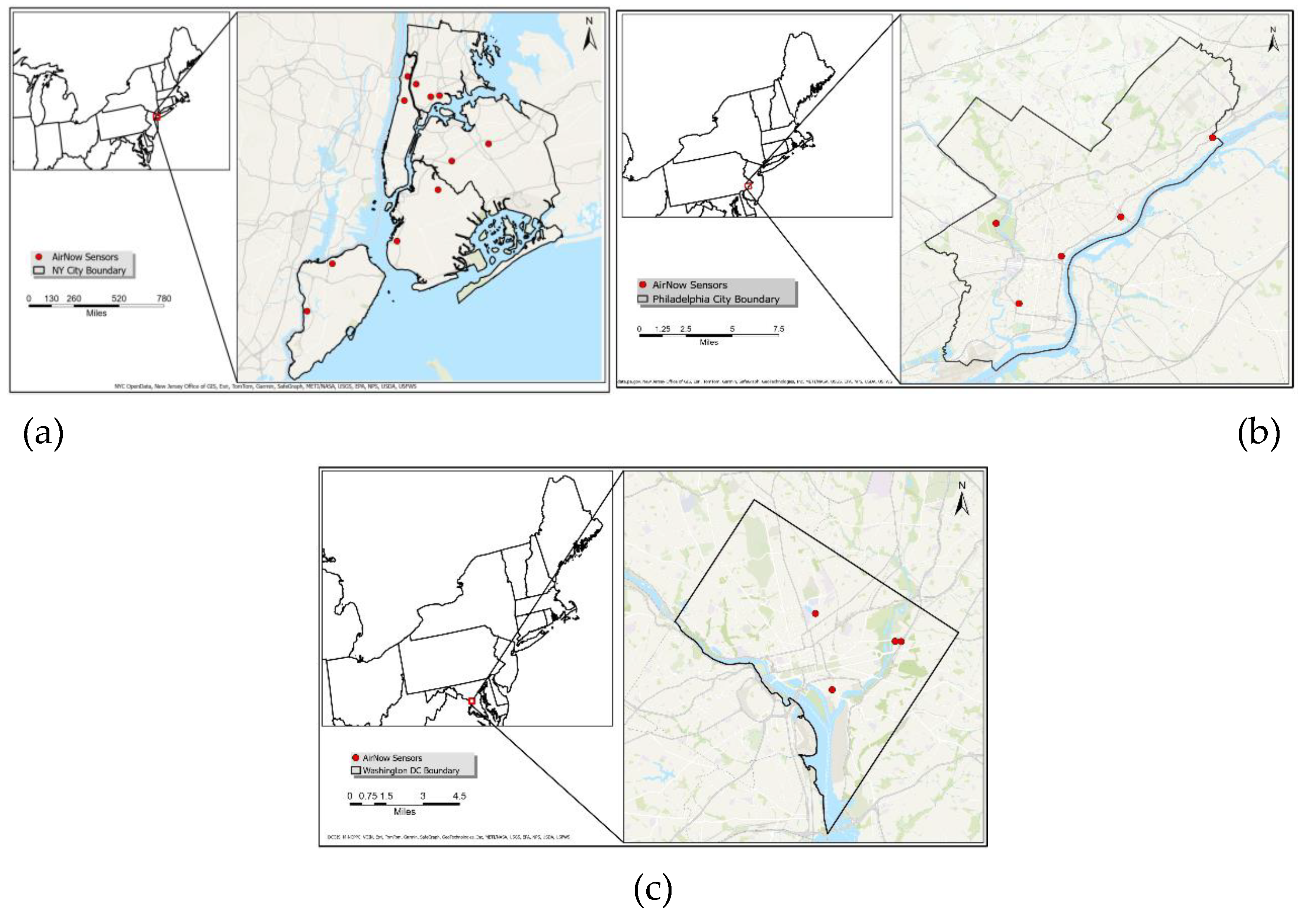
Figure 2.
Methodology Workflow Diagram.
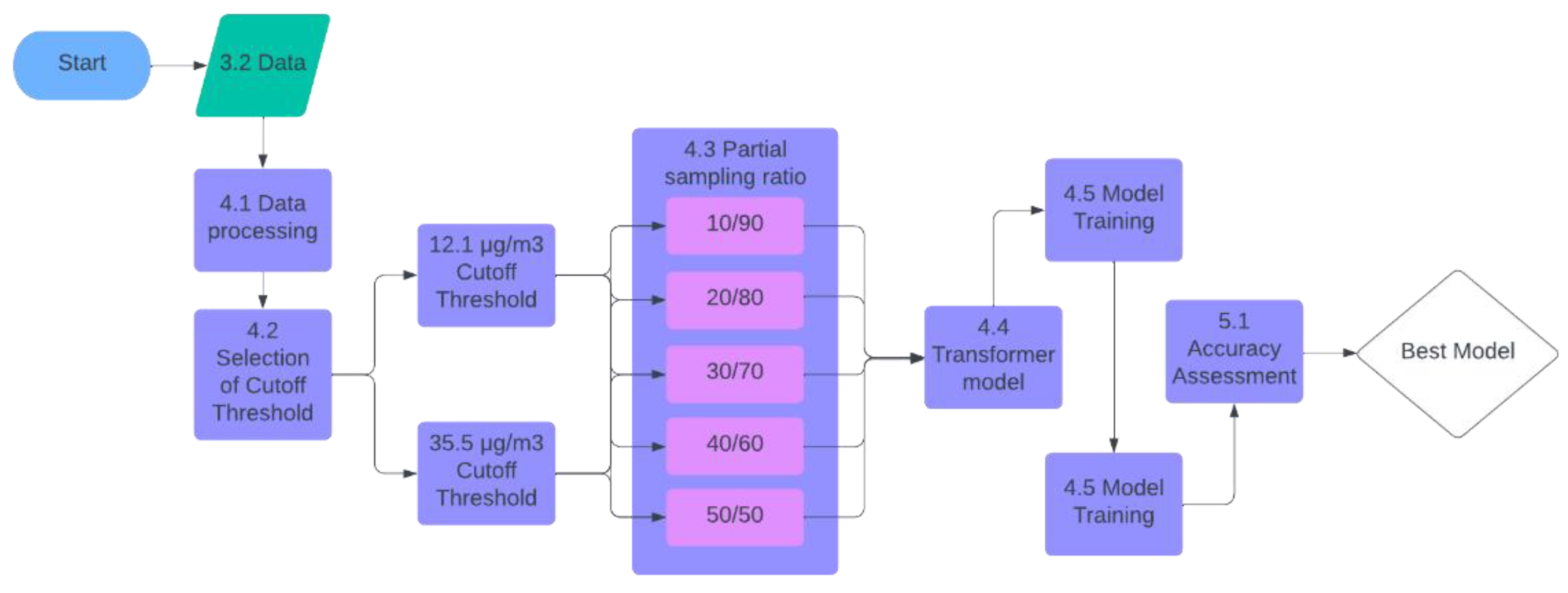
Figure 3.
Distribution of training dataset with cutoff threshold 12.1 µg/m³ and partial sampling ratio, from top left to bottom right, of none (original distribution), 10/90, 20/80, 30/70, 40/60, 50/50.
Figure 3.
Distribution of training dataset with cutoff threshold 12.1 µg/m³ and partial sampling ratio, from top left to bottom right, of none (original distribution), 10/90, 20/80, 30/70, 40/60, 50/50.
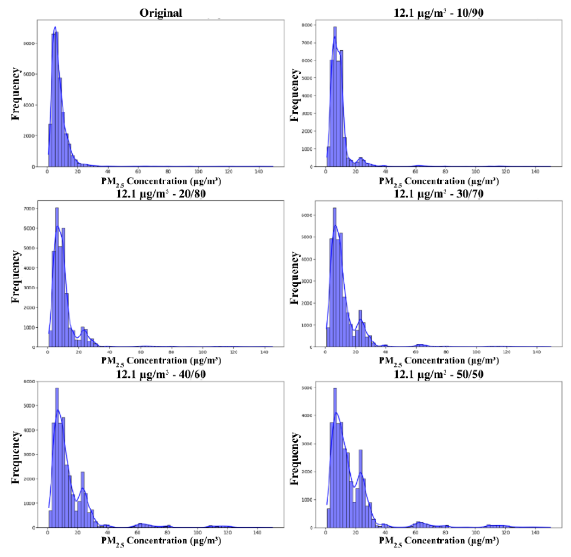
Figure 4.
Distribution of training dataset with cutoff threshold 12.1 µg/m³ and partial sampling ratio, from top left to bottom right, of none (original distribution), 10/90, 20/80, 30/70, 40/60, 50/50.
Figure 4.
Distribution of training dataset with cutoff threshold 12.1 µg/m³ and partial sampling ratio, from top left to bottom right, of none (original distribution), 10/90, 20/80, 30/70, 40/60, 50/50.
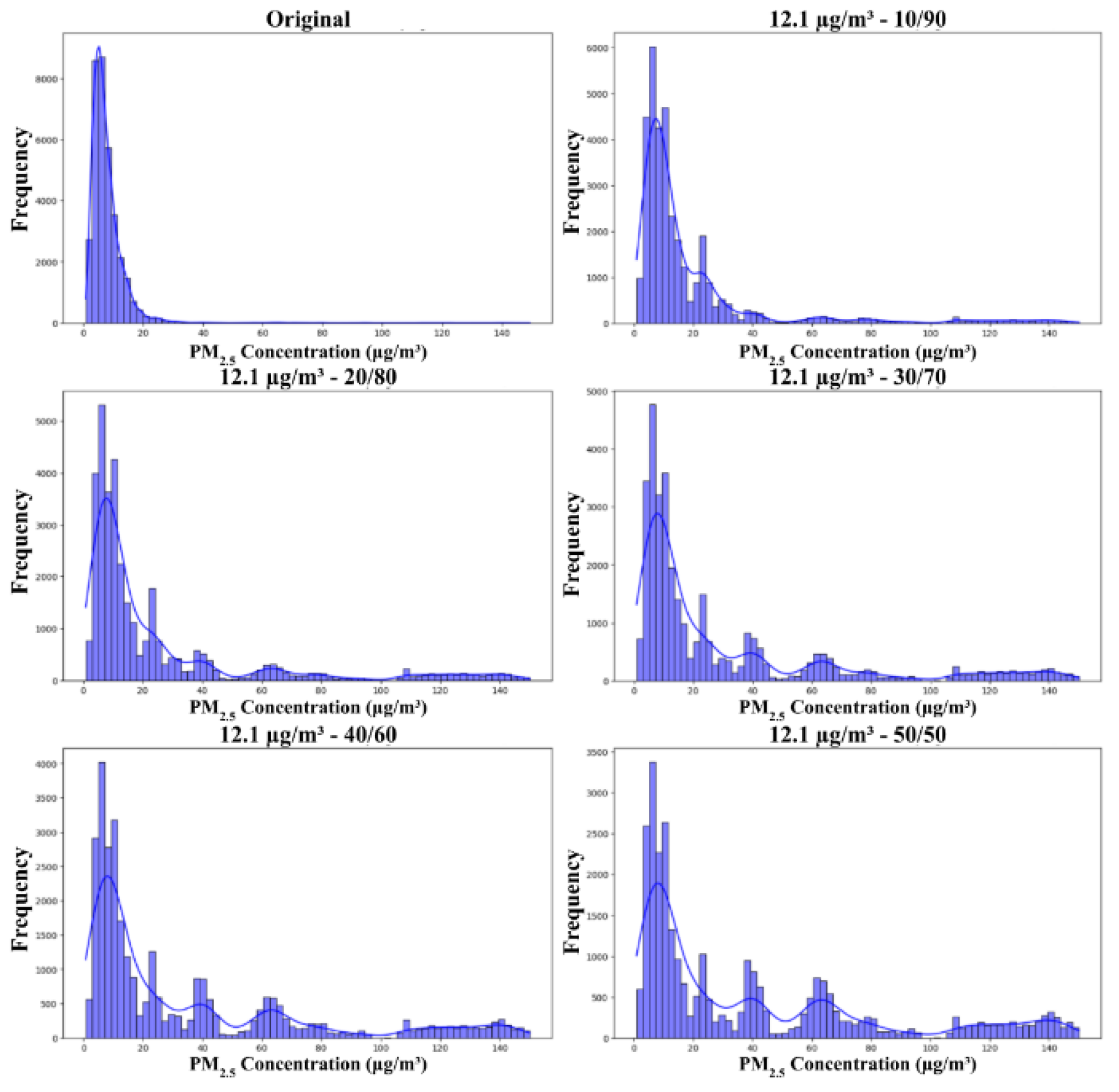
Figure 5.
Transformer model architecture.
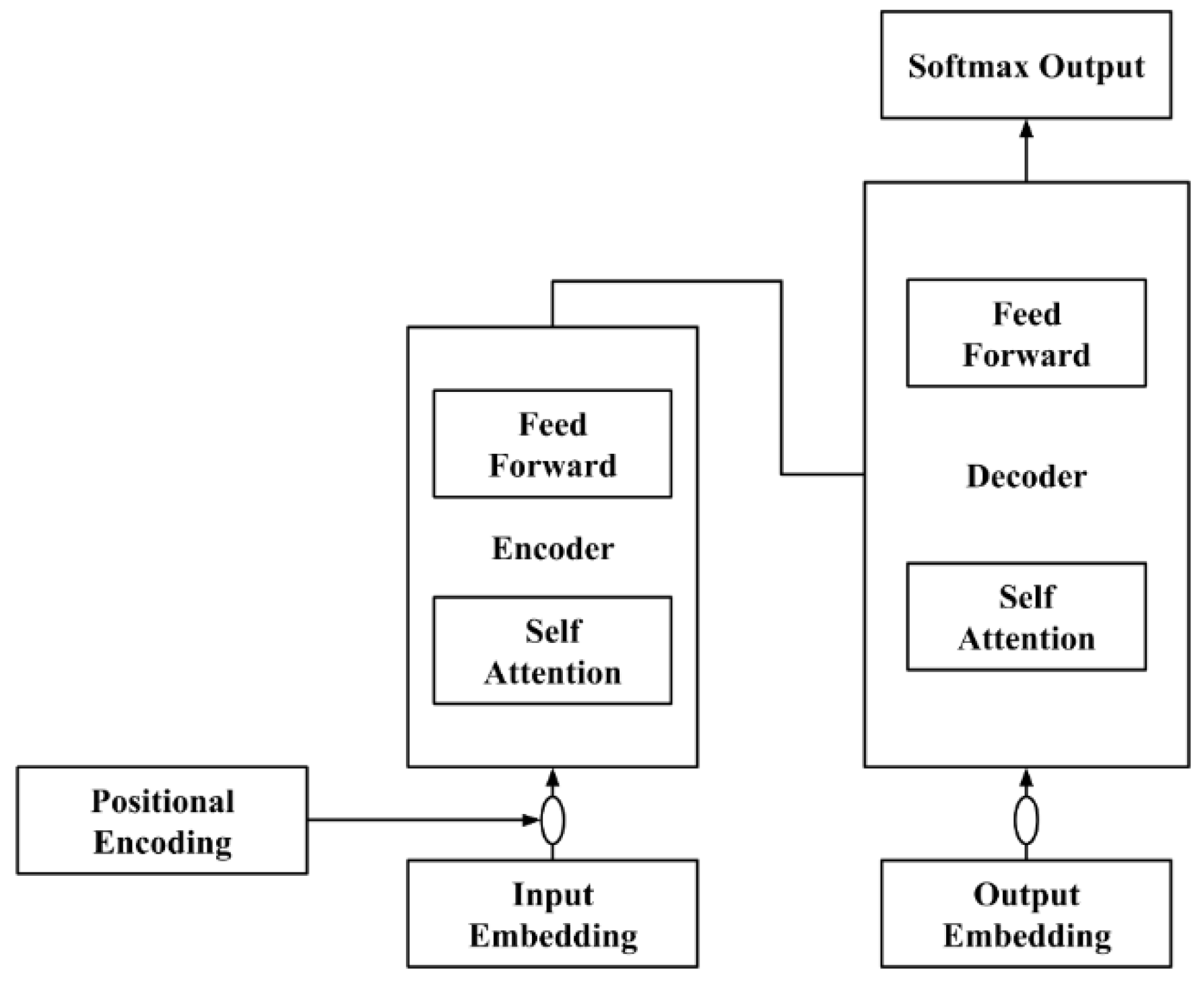
Figure 6.
RMSE (blue), MAE (green), and R² (red) performance metrics across various partial sampling ratios using the 12.1 µg/m³ threshold tested on whole (Left) and high-value (Right) testing datasets.
Figure 6.
RMSE (blue), MAE (green), and R² (red) performance metrics across various partial sampling ratios using the 12.1 µg/m³ threshold tested on whole (Left) and high-value (Right) testing datasets.
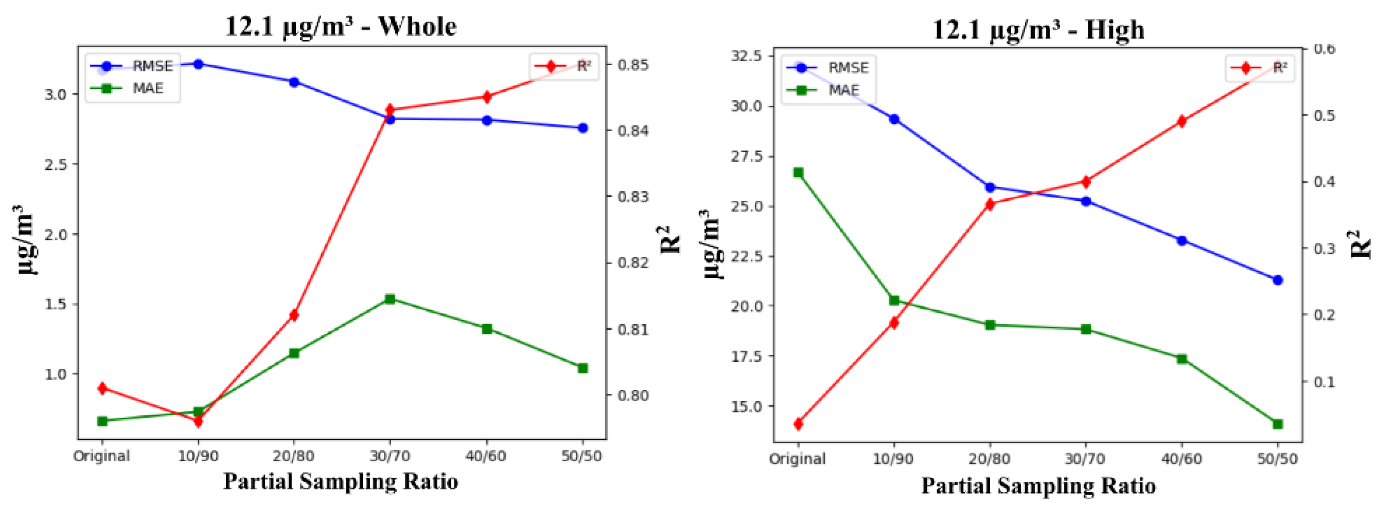
Figure 7.
RMSE (blue), MAE (green), and R² (red) performance metrics across various partial sampling ratios using the 35.5 µg/m³ threshold tested on whole (Left) and high-value (Right) testing datasets.
Figure 7.
RMSE (blue), MAE (green), and R² (red) performance metrics across various partial sampling ratios using the 35.5 µg/m³ threshold tested on whole (Left) and high-value (Right) testing datasets.
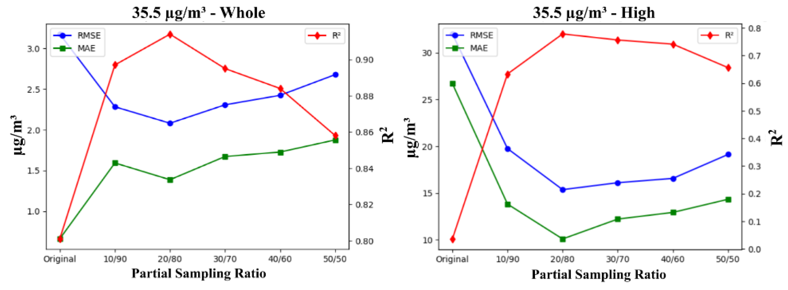
Figure 8.
RMSE, MAE, and R² performance metrics for the 12.1 µg/m³ (green) and 35.5 µg/m³ (blue) thresholds across partial sampling ratios.
Figure 8.
RMSE, MAE, and R² performance metrics for the 12.1 µg/m³ (green) and 35.5 µg/m³ (blue) thresholds across partial sampling ratios.
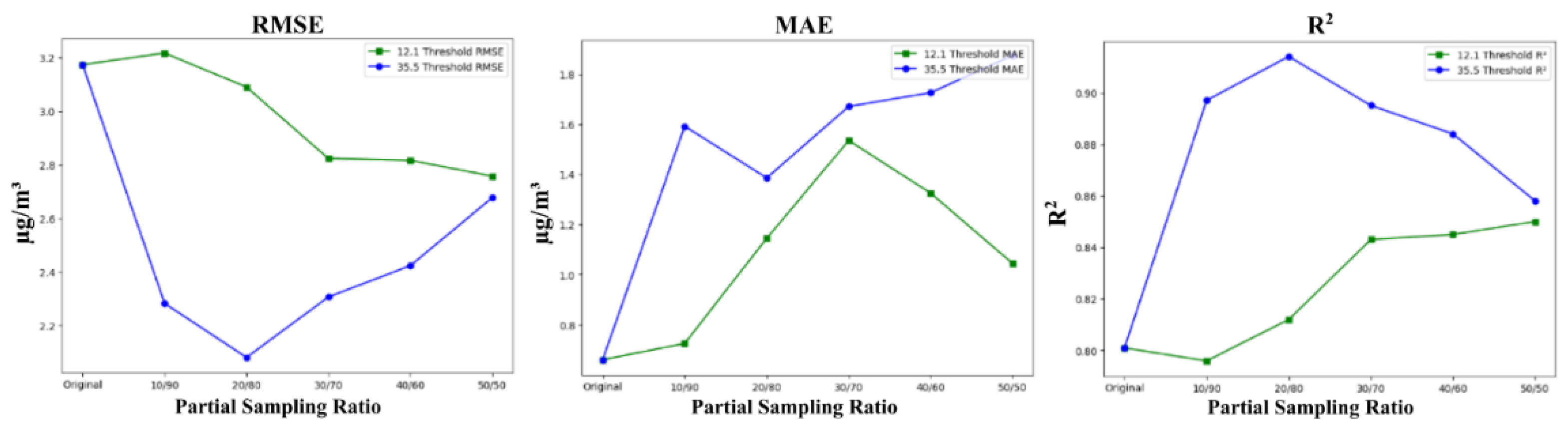
Figure 9.
Time series of observed (blue) and forecasted (orange) PM2.5 concentrations from 2021 to 2023 in New York City (top), Philadelphia (middle), and Washington D.C. (bottom). The left column shows predictions from model trained on original distribution and the right column shows predictions from model trained on data treated with optimal data augmentation determined in Section 5.1.
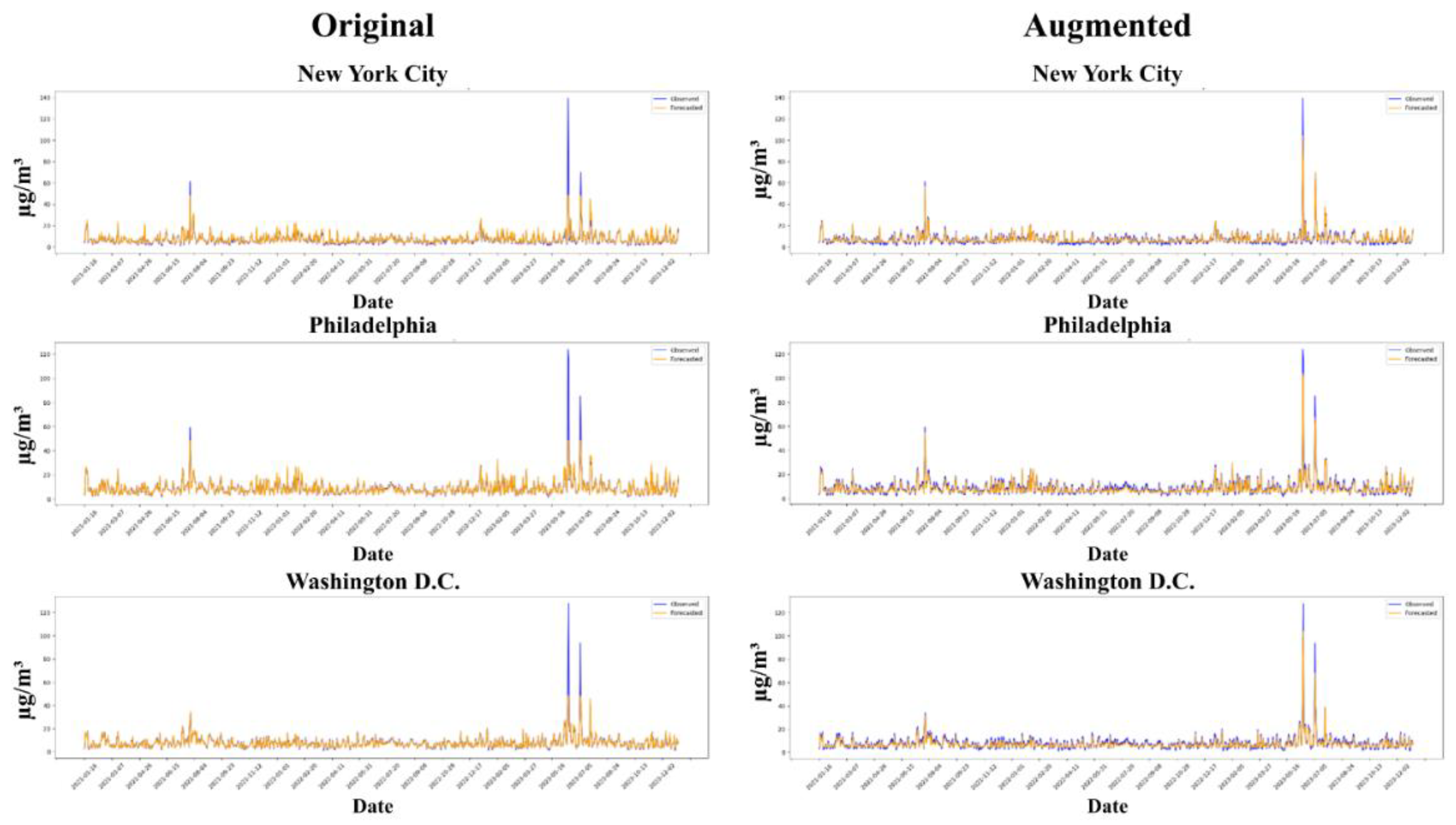

Table 1.
This study includes the area, population, and geographical location of the three cities.
| City | Area | Population | Coordinates |
|---|---|---|---|
| New York City | 790 square km (302.6 square miles) | 8.336 million | 40.4774° N, -74.2591° W (southwest) to 40.9176° N, -73.7004° W (northeast) |
| Philadelphia | 347.52 square km (134.18 square miles) | 1.567 million | 39.8670° N, -75.2803° W (southwest) to 40.1379° N, -74.9558° W (northeast) |
| Washington D.C. | 76 square km (68 square miles) | 671,803 | 38.7916° N, -77.1198° W (southwest) to 38.9955° N, -76.9094° W (northeast) |
Table 2.
Sources and units of variables used to forecast PM2.5.
| Variable | Type | Source | Unit |
| PM2.5 | Target | AirNow | μg/m³ |
| AOD | Covariate | MODIS MAIAC (Terra and Aqua) | Unitless |
| Boundary Layer Height | Covariate | ECMWF ERA5-hourly | meter |
| Relative Humidity | Covariate | ECMWF ERA5-hourly | % |
| Temperature (at 2m) | Covariate | ECMWF ERA5-hourly | K |
| Surface Pressure | Covariate | ECMWF ERA5-hourly | Pa |
| Wind Speed | Covariate | ECMWF ERA5-hourly | m/s |
| Elevation | Covariate | USGS | Meter |
Table 3.
Breakdown of low and high-value samples with 12.1 µg/m³ cutoff threshold.
| City | Total Samples | Low-Value | High-Value | Ratio of High to Low-Value |
|---|---|---|---|---|
| New York City | 2,284,200 | 2,038,105 | 246,095 | 0.1207 |
| Washington DC | 456,840 | 406,716 | 50,124 | 0.1232 |
| Philadelphia | 1,285,200 | 1,027,868 | 257,332 | 0.2503 |
| Total | 4,026,240 | 3,472,689 | 553,551 | 0.1594 |
Table 4.
Breakdown of low and high-value samples with 35.5 µg/m³ cutoff threshold.
| City | Total Samples | Low-Value | High-Value | Ratio of High to Low-Value |
|---|---|---|---|---|
| New York City | 2,284,200 | 2,272,914 | 11,286 | 0.00496 |
| Washington DC | 456,840 | 454,649 | 2,191 | 0.00481 |
| Philadelphia | 1,285,200 | 1,276,870 | 8,330 | 0.00652 |
| Total | 4,026,240 | 4,004,433 | 21,807 | 0.00544 |
Table 5.
Number of high and low-value samples in the training dataset at each partial sampling ratio.
Table 5.
Number of high and low-value samples in the training dataset at each partial sampling ratio.
| Partial Sampling Ratio | High-Value Samples | Low-Value Samples |
|---|---|---|
| 10/90 | 3,498 | 31,482 |
| 20/80 | 6,996 | 27,984 |
| 30/70 | 10,494 | 24,486 |
| 40/60 | 13,992 | 20,988 |
| 50/50 | 17,490 | 17,490 |
Table 6.
Hyperparameters used for model training.
| Training Parameter | Values |
|---|---|
| Model training data | 2021, 2022, 2023 |
| Data split | Training (80%) and testing (20%) |
| Optimizer | Adam |
| Learning Rate | 0.001 |
| Epochs | 20 |
| Number of encoder and decoder layers | 6 |
| Model Dimension | 8 |
| Batch Size | 256 |
| Input length | 8 |
| Output length | 8 |
| Dropout Rate | 0.1 |
Table 7.
Accuracy measurements of models trained on data augmented with cutoff threshold 12.1 µg/m³ and different partial sampling ratios tested on the whole and high-value testing dataset.
Table 7.
Accuracy measurements of models trained on data augmented with cutoff threshold 12.1 µg/m³ and different partial sampling ratios tested on the whole and high-value testing dataset.
| Resampling Ratio | Whole | High-Value | ||||
| RMSE | MAE | R² | RMSE | MAE | R² | |
| Original | 3.174 | 0.661 | 0.801 | 32.013 | 26.705 | 0.036 |
| 10/90 | 3.217 | 0.726 | 0.796 | 29.366 | 20.284 | 0.188 |
| 20/80 | 3.090 | 1.145 | 0.812 | 25.948 | 19.044 | 0.366 |
| 30/70 | 2.823 | 1.535 | 0.843 | 25.243 | 18.827 | 0.400 |
| 40/60 | 2.816 | 1.325 | 0.845 | 23.284 | 17.383 | 0.490 |
| 50/50 | 2.757 | 1.044 | 0.850 | 21.287 | 14.114 | 0.574 |
Table 8.
Accuracy measurements of models trained on data augmented with cutoff threshold 35.5 µg/m³ and different partial sampling ratios tested on the whole and high-value testing dataset.
Table 8.
Accuracy measurements of models trained on data augmented with cutoff threshold 35.5 µg/m³ and different partial sampling ratios tested on the whole and high-value testing dataset.
| Resampling Ratio | Whole | High-Value | ||||
| RMSE | MAE | R² | RMSE | MAE | R² | |
| Original | 3.174 | 0.661 | 0.801 | 41.34 | 28.269 | 0.607 |
| 10/90 | 2.282 | 1.592 | 0.897 | 19.747 | 13.81 | 0.633 |
| 20/80 | 2.080 | 1.386 | 0.914 | 15.353 | 10.077 | 0.778 |
| 30/70 | 2.306 | 1.671 | 0.895 | 16.095 | 12.204 | 0.756 |
| 40/60 | 2.423 | 1.726 | 0.884 | 16.556 | 12.917 | 0.741 |
| 50/50 | 2.677 | 1.875 | 0.858 | 19.116 | 14.321 | 0.656 |
Disclaimer/Publisher’s Note: The statements, opinions and data contained in all publications are solely those of the individual author(s) and contributor(s) and not of MDPI and/or the editor(s). MDPI and/or the editor(s) disclaim responsibility for any injury to people or property resulting from any ideas, methods, instructions or products referred to in the content. |
© 2024 by the authors. Licensee MDPI, Basel, Switzerland. This article is an open access article distributed under the terms and conditions of the Creative Commons Attribution (CC BY) license (http://creativecommons.org/licenses/by/4.0/).
Copyright: This open access article is published under a Creative Commons CC BY 4.0 license, which permit the free download, distribution, and reuse, provided that the author and preprint are cited in any reuse.


