

Submitted:
26 July 2024
Posted:
30 July 2024
You are already at the latest version
Abstract
This study focuses on predicting PM2.5 levels at the University of Petroșani by employing advanced machine learning techniques to analyze a dataset that encapsulates a wide array of air pollutants and meteorological factors. Utilizing data from IoT sensors and established environmental monitoring stations, the research leverages Random Forest, Gradient Boosting Machines, and Support Vector Regression models to forecast air quality, emphasizing the complex interplay between various pollutants. The models demonstrate varying degrees of accuracy, with the Random Forest model achieving the highest predictive power, indicated by an R2 score of 0.82764. Our findings highlight the significant impact of specific pollutants such as NO, NO2, and CO on PM2.5 levels, suggesting targeted mitigation strategies could enhance local air quality. Additionally, the study explores the role of temporal dynamics in pollution trends, employing time-series analysis to further refine the predictive accuracy. This research contributes to the field of environmental science by providing a nuanced understanding of air quality fluctuations in a university setting and offering a replicable model for similar environments seeking to reduce airborne pollutants and protect public health.
Keywords:
Environmental Monitoring
; Pollutant Analysis
; IoT Sensors
; Predictive Analytics
; Urban Sustainability
1. Introduction
As urbanization and industrialization continue to surge globally, air pollution emerges as a critical environmental and public health concern. The detrimental effects of air pollutants underscore the need for effective monitoring and prediction mechanisms, particularly in densely populated areas. Recent advancements in machine learning and artificial intelligence provide promising tools for tackling these challenges by enhancing the precision of air quality forecasts and facilitating effective management strategies.
Despite the extensive research focused on air quality assessment in major urban settings, some examples of air quality monitoring in specialized environments such as university campuses can be mentioned, as follows: University of Cambridge and University of Leeds are actively engaged in sustainability projects focused on air quality estimation. The University of Cambridge, through its Cambridge Green Challenge, incorporates air quality monitoring to inform campus planning and enhance environmental policies [1]. The University of Leeds has established the "Living Lab for Air Quality" which utilizes both fixed and mobile air quality monitoring to develop strategies that improve the campus environment and inform broader sustainability practices [2]. These areas are characterized by dynamic population shifts and diverse daily activities, which significantly influence local air quality levels. Traditional urban studies do not adequately capture the nuanced environmental impact driven by the academic settings' unique operational patterns. Hence, there is an acknowledged need to tailor research and develop predictive models that cater specifically to the environmental context of university campuses. Such targeted studies are crucial for safeguarding the health and well-being of the academic community and ensuring compliance with environmental standards.
This research aims to address this gap by predicting air quality within the University of Petroșani campus, focusing particularly on PM2.5 levels—recognized as a primary pollutant with extensive health implications. The region of Valea Jiului, historically known as a mono-industrial zone centered around coal mining, is currently undergoing significant transformations. As part of the broader European strategy for a Just Transition [3], this area is striving to align with rigorous environmental standards. The present study is integrated into this effort, leveraging detailed pollutant data and machine learning techniques to predict air quality. By doing so, it contributes to the broader initiative to mitigate environmental impacts and enhance air quality in transitional economies, particularly in regions adjusting from heavy industrial legacies to more diversified and sustainable frameworks.
Currently, the air quality in Petroșani, Romania, is classified as "Moderate" with a US AQI (Air Quality Index) of 53. The main pollutant affecting this rating is PM2.5, with a concentration of 10.2 µg/m3, which is twice the annual guideline value set by the World Health Organization [4]. This underscores the necessity of enhancing local air quality predictions to protect vulnerable populations and guide effective environmental governance.
The paper begins with a comprehensive literature review that contextualizes the current state of research in air quality prediction, followed by a detailed presentation of our research methodology in the "Materials and Methods" section. Subsequent sections focus on the specific challenge of predicting PM2.5 levels at the University of Petroșani campus. These sections detail the process from data collection and processing to the selection and training of machine learning models, supported by the key findings and results from our analysis.
2. Literature Review
This literature review presents the advancements in air quality prediction, the capabilities and applications of modern machine learning techniques, as emphasized in multiple studies. Traditional methods like numerical modeling and statistical analysis, while foundational, often fall short in capturing the complex, nonlinear relationships within air pollution data—a gap increasingly bridged by supervised machine learning algorithms.
Air quality prediction has traditionally relied on numerical modeling and statistical techniques. However, these methods often struggle to capture the complex and non-linear relationships inherent in air pollution data. Recent advances in machine learning, particularly supervised learning algorithms, have shown significant improvements in air quality prediction by leveraging large data sets and sophisticated analytical techniques. This literature review covers various machine learning approaches, including long-short-term memory (LSTM), random forest (RF), artificial neural networks (ANN), and support vector regression (SVR), highlighting their applications and effectiveness in air quality prediction.
Despite significant progress, challenges remain, including the need for robust data preprocessing, addressing data imbalance, and developing interpretable models. This review highlights the critical role of integrating machine learning with emerging technologies such as IoT and cloud computing to improve real-time air quality monitoring and decision making.
The paper by Die Tang et al [5] provides a comprehensive review of the use of machine learning models for estimating ground-level air pollutant concentrations. The study uses satellite data from sensors such as the Moderate Resolution Imaging Spectroradiometer (MODIS), the Ozone Monitoring Instrument (OMI) and the Troposphere Monitoring Instrument (TROPOMI) to complement measurements from ground-based monitoring stations. For example, aerosol optical depth (AOD) measurements from MODIS have been used to reveal spatial variations of PM2.5 fine particles. Machine learning models such as neural networks and Random Forests have been used to simulate the complex relationships between satellite variables and ground pollutant concentrations, providing essential data for air quality management and epidemiological studies. A notable example is a neural network model that predicted daily PM2.5 concentrations at 1 km resolution for the United States between 2000 and 2012. The paper proposes practical solutions to the identified problems and suggests future research directions, such as developing more robust data preprocessing strategies, addressing the problem of unbalanced data and implementing appropriate model validation and interpretation strategies to improve their generalizability and applicability in air quality mapping.
Zhang et al. [6] review air quality prediction methods, focusing on deep learning techniques. This highlights the importance of accurate predictions for public health and early warning systems. Initially, traditional methods such as regression models and Autoregressive Integrated Moving Average (ARIMA) models were used, but they had limitations in capturing pollutant dynamics. Later, techniques such as support vector regression and random forests provided better results, but not sufficiently accurate for complex long-term relationships. Deep learning techniques such as convolutional neural networks and recurrent neural networks have made significant improvements. For example, Long Short-Term Memory (LSTM) and Gated Recurrent Unit (GRU) networks handle long-term dependencies, and Convolutional Neural Networks (CNNs) capture spatial features. The study compares these methods and highlights the superiority of deep learning in modeling complex relationships and handling large volumes of data. The authors discuss the use of attention mechanisms such as the Transformer architecture, which improves predictions by modeling long-term relationships without sequence length constraints. The paper highlights the importance of advanced data preprocessing and integrates spatiotemporal information for accurate results. It also highlights the need to develop more robust and interpretable models to address computational complexity. The paper highlights the crucial role of deep learning in air quality prediction and suggests future research directions to improve the generalizability and performance of models, including through transfer learning techniques and the development of integrated models that combine the advantages of traditional and deep learning methods.
In the context of rapid urbanization and severe pollution in Delhi, India, [7] explores the influence of air quality awareness on transport choices using machine learning models. The authors collected data from 346 survey respondents and analyzed how air pollution influences travel behavior. Models used include Random Forest, XGBoost, Naive Bayes, K-Nearest Neighbor, Support Vector Machine and Multinomial Logistic Regression. The study showed that Random Forest had the highest accuracy in predicting travel behavior. As air quality deteriorates, travelers prefer closed modes of transport (air-conditioned cars, subways) to open modes (walking, bicycles) and choose public transport over private transport due to ventilation and air filtration. Air quality awareness is critical to travel decisions. The authors emphasize the importance of disseminating air quality information and recommend integrating this information into transportation planning to promote sustainable modes of transportation and reduce exposure to pollution. The paper suggests using machine learning to investigate causal relationships and develop effective strategies to reduce exposure to pollution. It also emphasizes the need for greater public education on the health risks associated with air pollution and the benefits of green transportation.
Machine learning techniques are often applied alongside secondary modeling to enhance traditional air quality index (AQI) predictions as innovative air quality prediction methods. Utilizing data from Jinan, China, including forecasts and observed pollutant concentrations, the study applies machine learning models like Light Gradient Boosting Machine (LightGBM) and Long Short-Term Memory (LSTM), achieving high accuracy and reliability in predicting AQI and specific pollutants like ozone. The research [8] underscores the critical role of incorporating meteorological data and advanced data preprocessing in developing robust prediction models, paving the way for future advancements in environmental monitoring. This highlights the potential of machine learning to significantly improve the precision and applicability of air quality forecasts.
A novel air pollution prediction method using a Gaussian mixture knotted factorial variational autoencoder (NF-VAE), designed to tackle the complexities of multivariate pollution data effectively is introduced in paper [9]. This model surpasses traditional machine learning and deep learning approaches by providing accurate, simultaneous predictions for various pollutants. Utilizing data from six monitoring stations in China, the NF-VAE model demonstrates remarkable improvements in prediction accuracy over other models, highlighted by significant advancements in statistical measures like RMSE, MAE, and R2. This research underscores the potential of NF-VAE to enhance air quality forecasts by adeptly managing complex, multivariate datasets, suggesting directions for future enhancements including advanced data preprocessing and model scaling to better capture the diverse dynamics of air pollution.
The study by Manzoor Ansari and Mansaf Alam [10] introduces an advanced air quality prediction model, the BO-HyTS, which integrates IoT devices with cloud technology using a hybrid approach of SARIMA and LSTM models to address both linear and nonlinear aspects of air quality data. This model leverages Bayesian optimization for fine-tuning, leading to superior performance in key metrics like MSE, RMSE, and MAE compared to other models. The research emphasizes the synergy of IoT, cloud computing, and sophisticated time series analysis, highlighting their potential in enhancing real-time air quality monitoring and decision-making processes. This integration facilitates effective pollution management and public health protection by providing timely and accurate air quality predictions.
Aram et al. [11] explore various machine learning models to predict Air Quality Index (AQI) and Air Quality Grade (AQG) using data from 2014-2019 on six key pollutants. The study evaluates models such as Random Forest, Gradient Boosting, and Lasso Regression for AQI, and models like K-Nearest Neighbors and Support Vector Machines for AQG. Superior performance was noted in stacked models for both AQI and AQG predictions, demonstrating higher accuracy and robustness compared to individual models. This highlights the effectiveness of using advanced ensemble techniques in air quality forecasting.
The work by Ankita Mishra and Yogesh Gupta [12] explores the efficacy of deep learning and classical machine learning methods in predicting the Air Quality Index (AQI). They compare LSTM and ARIMA models, highlighting LSTM's superior performance for hourly AQI predictions due to its advanced capabilities in handling complex sequential data. The study also evaluates other models like Decision Trees and XGBoost, with a focus on LSTM's lower RMSE for hourly data, emphasizing its suitability for dynamic urban environments. This research underscores the potential of integrating various predictive models to enhance AQI forecasting accuracy.
The paper [13] provides a comprehensive review of supervised machine learning methods for air pollution prediction amidst growing urbanization and industrial activities. Utilizing the PRISMA method for literature organization, it explores how algorithms like LSTM, Random Forest, ANN, and SVR are applied to predict critical pollutants like PM, NOx, CO, and O3. It underscores the integration of ICT with machine learning for real-time air quality monitoring, addresses challenges such as sensor reliability and privacy, and emphasizes adapting IoT-based systems to local contexts for effective air quality management.
Shoukry, F. et al. [14] explore the interplay between indoor air quality (IAQ) and energy consumption in university classrooms, particularly under the constraints of the COVID-19 pandemic. Utilizing Grasshopper software on Rhino Version 7, the study models the impact of various factors such as occupancy, room volume, and ventilation rates on energy use for mechanical ventilation. Their findings highlight significant opportunities for optimizing energy efficiency while maintaining healthy IAQ levels, offering a vital resource for facility managers aiming to enhance sustainability and cost-effectiveness in educational environments.
There is not much specific work on the prediction of air quality in outdoor areas of university campuses. Most studies focus on air quality prediction in large cities or dense urban areas where air pollution is a major problem. An example is the study by Huiping Peng at the University of British Columbia, which used machine learning methods for air quality prediction, but did not focus exclusively on university campus areas [15]. Other studies discuss air quality monitoring on university campuses, but without emphasizing the specific prediction of outdoor air quality in these areas [16] or use geographically weighted regression to map the spatial variability of PM2.5 pollution and identify its key determinants, focusing on the campus setting, emphasizing the importance of localized data and modeling to enhance air quality prediction and inform sustainable practices on university campuses [17].
This highlights a significant research gap in the field. There is a clear need for studies dedicated to the prediction of air quality in outdoor areas of university campuses, given the particularities of these environments, such as frequent fluctuations in the number of people and various activities that can affect air quality. Exploring this area could significantly contribute to improving the health and well-being of the university community by implementing air quality management strategies based on accurate and up-to-date data.
3. Materials and Methods
The methodology for this research, aimed at predicting PM2.5 levels in the University of Petroșani campus is presented in Figure 1. Each section contributes systematically towards building a robust predictive model using machine learning techniques.
The state of the art involves a comprehensive review of existing literature on air quality prediction, particularly focusing on studies conducted in urban areas and other environments similar to university campuses. This review highlights advancements in machine learning applications for air quality monitoring and prediction, setting the stage for identifying innovative approaches and technologies that can be adapted to our specific setting.
The research identifies existing gaps, particularly the lack of focused studies on air quality in university settings, which have unique characteristics different from urban centers. The problem is formulated around the need to predict PM2.5 levels, which are critical for health but not adequately monitored on smaller scales like a university campus. The goal is to develop a predictive model that can provide real-time insights into air quality, allowing for proactive management measures to safeguard the health of the university community.
Data collection involves gathering historical air quality data specific to the University of Petroșani and its surrounding areas. This includes pollutants such as CO, O3, NO, NO2, and SO2, alongside PM2.5 levels. Additional data include meteorological conditions, like relative humidity (RH) and temperature (Temp), as these significantly influence pollutant levels.
Before model development, the dataset is undergoing thorough analysis to understand the distribution of variables, detect outliers, handle missing values through interpolation, and explore correlations between the predictors and the target variable, PM2.5. This step ensures that the machine learning model will be trained on clean, comprehensive, and relevant data, crucial for ensuring the accuracy and reliability of the predictions.
Selection of the machine learning model is based on the dataset characteristics and the insights gained from the dataset analysis phase. Considering the non-linear relationships and interactions among variables, ensemble methods like Random Forest and Gradient Boosting Machines are considered. These models are known for their robustness and ability to handle complex datasets with mixed-type data and interactions.
The model is trained using the prepared dataset, with a focus on optimizing parameters such as the number of trees and minimum leaf size in the case of Random Forest, or learning rate and number of boosting stages for Gradient Boosting. Training involves partitioning the data into training and validation sets to monitor for overfitting and ensure the model generalizes well to new data.
Post-training, the model’s performance is evaluated using appropriate metrics, primarily the R2 score to measure how well the model predictions match the observed data. Additional metric, Mean Absolute Error (MAE), is used to provide further insights into the model's accuracy and precision.
This structured approach ensures that the model developed is not only scientifically rigorous but also tailored to the specific needs of the University of Petroșani, ultimately aiming to enhance campus health and environmental safety.
For the research focused on predicting PM2.5 levels on the University of Petroșani campus using advanced machine learning techniques, the following specific objectives were identified:
1. To review existing literature on air quality prediction in order to understand the current state of air quality prediction methodologies, with a particular focus on urban and campus environments.
2. To develop a robust dataset for model training, compile and preprocess it. This includes handling missing data, detecting and addressing outliers, and ensuring the dataset is comprehensive and representative.
3. To select and optimize suitable machine learning models for accurately predicting PM2.5 levels.
4. To validate the model's predictive accuracy using statistical metrics such as R2 and MAE.
These objectives address the immediate need for accurate air quality prediction at the University of Petroșani and contribute to broader efforts in environmental protection and public health promotion. By fulfilling these objectives, the research provides a template for similar studies in other contexts and help in formulating more effective environmental policies.
4. Air Quality Prediction Problem for the University of Petroșani Campus
To effectively address the challenge of predicting air quality for the University of Petroșani campus, a comprehensive approach is required that leverages advanced data collection techniques, machine learning models, and state-of-the-art technological infrastructure. The unique environmental conditions and specific characteristics of the university campus necessitate a tailored approach that seamlessly integrates both local and broader regional data sources.
Data collection forms the cornerstone of our methodology in developing a robust air quality prediction model. By utilizing existing monitoring data from the Jiu Valley, particularly insights from studies conducted by INSEMEX Petroșani, we establish a solid foundation. These studies have identified key pollutants—particulate matter (PM10, PM2.5), nitrogen dioxide (NO2), sulfur dioxide (SO2), carbon monoxide (CO), and ozone (O3)—as critical indicators of air quality in the region. This historical data provides invaluable benchmarks and trends essential for model calibration. [18]
Further enhancing our data collection, we deploy Internet of Things (IoT) sensors across the university campus and surrounding areas. These sensors are equipped to continuously monitor the same set of pollutants, alongside crucial meteorological parameters such as temperature and humidity. This integration of IoT technology ensures that our dataset is not only comprehensive but also dynamic, capturing real-time environmental changes. The deployment of these sensors creates a dense network that offers granular insights into the spatial variability of air quality, crucial for pinpointing localized pollution sources and understanding their temporal dynamics.
Our technological infrastructure is specifically designed to support extensive environmental monitoring and data analysis. The IoT sensors deployed are capable of measuring the seven key environmental parameters identified as inputs for our predictive model. These sensors are connected to a central data management system that processes and analyzes the data in real time. This system is equipped with advanced computational capabilities to handle the large volumes of data generated, ensuring data integrity and reliability through rigorous quality control measures.
The core of our predictive strategy involves developing machine learning models that can accurately forecast air quality levels based on the collected data. We explore several models to identify the most effective approach for our specific context. Random Forest utilizes multiple decision trees to make predictions, offering robustness and reliability. It is particularly effective in handling non-linear data and provides important insights into feature importance, helping us understand pollutant impact. Gradient Boosting Machines (GBM) improves prediction accuracy through iterative corrections of mistakes from previous trees. It is known for its effectiveness in dealing with diverse datasets and complex variable interactions, making it suitable for our comprehensive dataset. Support Vector Regression (SVR) is known for its effectiveness in high-dimensional spaces, with a focus on regression tasks help in fine-tuning our predictions to minimize errors.
By harnessing the strengths of these models, we aim to develop a hybrid approach that combines their predictive powers, enhancing accuracy and reliability.
5. Data Analysis
In the process of preparing the dataset for analysis, a systematic approach was adopted to address the presence of missing data, which were represented by zeros in the dataset. To handle the missing values, linear interpolation was utilized, a method that estimates missing entries based on linear relationships between known data points. This technique was applied column by column, identifying non-missing values and using these to interpolate values for the missing data points. This choice of interpolation preserves the continuity and trends inherent in the dataset, avoiding the introduction of bias that simpler methods such as mean imputation might cause. After filling in the missing values, the array was converted back into a table format, ensuring that the dataset was ready for further analysis or model training without losing the structural and relational integrity of the data. This approach helped maintain the quality and usability of the dataset, crucial for accurate and reliable subsequent analyses.
Based on the boxplot from Figure 2 for input variables in the dataset (CO, O3, RH, Temp, NO, NO2, SO2), the analysis regarding the distribution and potential issues in the data is further outlined.
CO (Carbon Monoxide) shows a very narrow interquartile range (IQR) close to zero, suggesting low variability among most values. There are no visible outliers, indicating stable and low variation across the observations. O3 (Ozone) exhibits a slightly wider IQR than CO, but it still remains relatively tight, centered at lower values. There are a few outliers, indicating occasional high ozone levels. RH (Relative Humidity) has a wider IQR compared to CO and O3, indicating more variability in humidity levels. The data points are clustered towards the upper range, and outliers are present on both the lower and upper ends, suggesting occasional extreme humidity conditions. Temp (Temperature) displays a symmetric distribution with a moderate spread in the IQR, centered around the median. There are multiple outliers on both the lower and upper ends, which may indicate unusual temperature readings or errors in data collection. NO (Nitric Oxide) has a wide spread in its IQR and several extreme values as outliers, indicating significant variation in nitric oxide levels and frequent high emissions events. NO2 (Nitrogen Dioxide), similar to NO, shows a relatively wide IQR with numerous outliers. This suggests variability in the data with frequent higher than typical nitrogen dioxide levels. SO2 (Sulfur Dioxide) shows a tight IQR but a significant number of outliers above the upper whisker. This indicates that while most SO2 levels are low, there are instances of very high emissions.
The presence of outliers, particularly in the NO, NO2, and SO2 variables, could be indicative of pollution events or data measurement errors. After further investigation it was determined that the outliers are due to actual extreme values that need to be modeled. Variables like RH and Temp show more natural variability and are less skewed than others. Given the skewness and presence of outliers, we consider using models that are less sensitive to outliers, such as tree-based models or robust regression methods.
Based on the histograms for each variable (CO, O3, RH, Temp, NO, NO2, SO2, and PM2.5) in Figure 3 the analysis of the dataset's distribution and characteristics is presented.
The histogram for CO shows a right-skewed distribution, indicating higher frequencies of lower concentration values, with a tail extending towards higher concentrations. This suggests that most of the time, CO concentrations are relatively low, with fewer occurrences of higher values. O3 concentrations appear to be somewhat uniformly distributed across a range, with a slight right skew. There are noticeable spikes around 40 and 100 units, indicating common specific values or ranges for ozone concentration. The histogram for RH shows a left-skewed distribution, with most data points concentrated towards higher humidity levels. This suggests that high humidity conditions are more common in the dataset. Temperature data appears to have a roughly normal distribution with a slight right skew, centered around 5 degrees. This indicates a moderate climate with variations extending towards warmer temperatures. The histogram for NO is heavily right-skewed, suggesting that low concentrations of NO are very common, with few higher readings. The NO2 distribution is also right-skewed but less so compared to NO. It indicates higher occurrences of moderate levels with a gradual decline towards higher concentrations. SO2 concentrations show a bimodal distribution with two peaks around 10 and 25 units. This might indicate two common conditions or sources impacting SO2 levels. PM2.5 levels are right-skewed, with most of the data concentrated at lower concentrations and fewer instances of higher concentrations. This suggests occasional high pollution events amidst generally low particulate matter levels.
Most pollutants (CO, NO, NO2, PM2.5) show right-skewed distributions, typical for environmental data where extreme pollution events are less frequent but significant. The presence of spikes or specific ranges in O3 and SO2 might indicate specific environmental conditions or emissions sources that recurrently influence these readings.
Beyond individual distributions, understanding how these variables interact—such as correlating pollutant levels with weather conditions (temperature and humidity)— provides insights into causal relationships and prediction models.
Based on the correlation matrix from Figure 4, we can derive insights into how these variables interact with each other.
CO and O3 have a correlation of -0.7826, that mean a strong negative correlation. As CO levels increase, O3 levels tend to decrease. This might be indicative of chemical interactions in the atmosphere where CO could be consuming ozone or related to varying sources of these emissions. O3 and Temp have a correlation of 0.7067, that is a strong positive correlation. Higher temperatures are associated with increased levels of ozone. This relationship is typical in urban environments where warmer temperatures can enhance ozone formation. RH and Temp have a correlation of -0.6827, that is a strong negative correlation. As temperatures rise, relative humidity tends to decrease, which is typical given that warmer air can hold more moisture before it condenses. RH and O3 have a correlation of -0.7466, that is a strong negative correlation. Increased humidity appears to be associated with lower ozone levels, possibly due to humidity's role in accelerating the decomposition of ozone. NO2 and NO have a correlation of 0.7349, that is a strong positive correlation. This relationship is expected as NO and NO2 are both nitrogen oxides and often emitted from the same sources, such as combustion processes. SO2 and CO have a correlation of 0.3651, that is a moderate positive correlation. This might indicate that some sources emitting CO are also emitting SO2.
The correlation between NO and NO2 suggests common sources, likely vehicular emissions or industrial combustion. The negative correlation between CO and O3 might be explored further to understand atmospheric chemistry, especially how pollutants interact under different environmental conditions. On days with higher forecast temperatures, additional measures might be necessary to control ozone levels. Correlations involving particulate matter (not shown directly here but can be inferred) and gases like NO2 and SO2 are particularly important, as these pollutants have direct health impacts.
This correlation matrix is a powerful tool for unveiling the interdependencies among air pollutants and can significantly enhance understanding and management of air quality issues.
6. Machine Learning Model
The correlation matrix from Figure 5 visualizes the relationships between various air pollutants and meteorological factors (CO, O3, RH, Temp, NO, NO2, SO2) and their association with PM2.5 levels.
CO correlation with PM2.5 is mildly positive and suggests that higher levels of CO might be associated with higher concentrations of PM2.5. This is indicative of common sources such as vehicle emissions or incomplete combustion processes contributing to both pollutants. O3 correlation with PM2.5 is mildly negative and indicates that higher ozone levels tend to coincide with lower PM2.5 concentrations. This reflects complex atmospheric chemistry where ozone, a secondary pollutant, does not directly emanate from the same sources as primary particulate matter or may even participate in atmospheric reactions that reduce particulate matter. RH correlation with PM2.5 is mildly positive and suggests that higher humidity levels might slightly enhance PM2.5 concentrations. This is due to increased hygroscopic growth of particulate matter under more humid conditions, causing particles to become heavier and more detectable. Temp correlation with PM2.5 is slightly negative and indicates that higher temperatures reduce PM2.5 levels, through enhanced dispersion in the atmosphere or decreased usage of heating sources which contribute to particulate emissions. NO correlation with PM2.5 is very slight positive and suggests a minor relationship where higher NO emissions could correlate with increased PM2.5, due to common urban sources such as traffic. NO2 correlation with PM2.5 is moderately positive, is a stronger positive correlation compared to NO, and suggests a more direct association or co-emission of NO2 with sources of particulate matter. This is typical of urban environments where vehicle emissions contribute significantly to both NO2 and PM2.5 levels. SO2 correlation with PM2.5 is mildly positive and indicates that sources emitting SO2, such as power plants and other industrial combustion processes.
The correlation matrix highlights several important environmental insights. Strong correlations (both positive and negative) provide evidence of shared emission sources or chemical interactions in the atmosphere, which can significantly affect air quality management strategies. For instance, the control strategies targeting NO2 might also effectively reduce PM2.5 levels due to their positive correlation.
In practical terms, understanding these correlations can aid policymakers in devising more comprehensive air quality management plans. For instance, measures to reduce vehicle emissions could be effective in simultaneously lowering levels of NO, NO2, CO, and indirectly PM2.5. Furthermore, this analysis underscores the importance of considering meteorological conditions in air quality models, as factors like temperature and humidity evidently influence pollutant concentrations.
In the context of predicting PM2.5 levels from a set of pollutants (CO, O3, RH, Temp, NO, NO2, SO2), the Random Forest model demonstrated robust performance with an R2 score of 0.82764. This ensemble learning technique builds multiple decision trees during training and outputs the mean prediction of the individual trees. Random Forest is particularly suitable for this task due to its ability to handle nonlinear relationships and interactions among features without requiring extensive data preprocessing. It also offers advantages in handling overfitting through its ensemble approach, where each tree is trained on a subset of data and features. This makes it highly effective for environmental datasets, which typically involve complex and noisy data structures.
The Gradient Boosting Machine (GBM) for predicting PM2.5 levels yielded an R2 score of 0.71755, utilizing 200 trees, a learning rate of 0.05, and a maximum of 20 splits per tree. GBM is a powerful and flexible machine learning technique that builds trees sequentially, with each new tree correcting errors made by previously trained trees. This additive model enhances prediction accuracy progressively but requires careful tuning of parameters like the number of trees, learning rate, and tree complexity to avoid overfitting. In environmental science, where predictor variables may have complex and subtle effects on outcomes, GBM's iterative approach can incrementally improve model performance, particularly useful in scenarios with changing or seasonal air quality patterns.
Support Vector Regression (SVR) applied to the same problem achieved an R2 score of 0.47955, indicating a moderate level of predictive accuracy compared to ensemble methods. Utilizing a linear kernel with a Box Constraint of 10 and an Epsilon of 10, SVR focuses on finding a decision surface that best fits the data within a certain threshold. While SVR is highly effective in high-dimensional spaces and for datasets where the margin of errors needs strict control, its performance in this instance suggests that the linear kernel may be too simplistic to capture the complex nonlinear relationships present in environmental data. This model's strength lies in its ability to provide robust predictions resistant to outliers, but it may require exploring non-linear kernels or additional feature engineering to improve its efficacy for air quality modeling.
The data analysis segment of this study comprehensively examined the relationships between various air pollutants and meteorological factors, utilizing a detailed correlation matrix that highlighted how these variables interact with PM2.5 levels. The analysis revealed associations, with some pollutants showing a direct correlation with PM2.5, while others exhibited inverse relationships. Notably, pollutants such as CO, NO2, and SO2 demonstrated positive correlations, suggesting common emission sources that contribute to higher PM2.5 levels. Conversely, O3 showed a negative correlation, indicating its complex role in atmospheric chemistry that might help reduce particulate levels under certain conditions. By identifying specific pollutants that strongly influence PM2.5 levels, this research underscores the potential for focused interventions that could simultaneously address multiple pollutants, thereby enhancing air quality more effectively. Moreover, this analysis lays a solid foundation for the predictive modeling phase, where machine learning techniques like Random Forest, Gradient Boosting Machine, and Support Vector Regression are employed to forecast PM2.5 concentrations. Each model's performance, reflected in their respective R2 scores, provides a comparative analysis into their suitability for handling the complex environmental data characteristic of this research, guiding further refinements in model selection and optimization for future studies.
7. Results and Discussion
In the tuning process for the Random Forest model aimed at predicting PM2.5 levels, a structured approach was utilized to explore a well-defined grid of parameters. Specifically, the number of trees and the minimum leaf size were varied to determine the optimal configuration. The number of trees considered were from the set [50, 100, 300, 500, 600, 700], providing a range from a moderately small to a large forest size, allowing for an assessment of how model complexity influenced performance as more trees can capture more complex patterns and reduce overfitting through averaging. The minimum leaf sizes tested were [1, 3, 5, 10], which explored a spectrum from very fine-grained (potentially high variance) to more generalized leaf configurations. This range was intended to see how much detail the model needed to capture to effectively predict PM2.5 levels, balancing between underfitting and overfitting.
The best parameters obtained from this grid were 500 trees and a minimum leaf size of 1. This outcome indicates that a high level of model complexity (many trees) combined with very detailed splits (small leaf size) provided the best performance, achieving an R2 value of 0.82764. Such a result suggests that the PM2.5 levels in this dataset are influenced by complex interactions among pollutants that require a dense model to capture accurately without overfitting, despite the granularity allowed by the smallest leaf size. This approach highlights the importance of rigorous parameter tuning in building effective predictive models, especially in environmental science where interactions can be highly non-linear and influenced by numerous factors.
Achieving an R2 score of 0.827640 with a Random Forest model using 500 trees and a minimum leaf size of 1 for predicting PM2.5 levels based on seven other pollutants is a strong result. This score indicates that the model explains about 82.76% of the variance in PM2.5 levels from the predictors used, which suggests that the model is highly effective for this task.
Using 500 trees in the Random Forest contributed significantly to capturing the complex relationships and interactions among the input variables. This high number of trees helps in averaging out the biases and reducing variance, leading to a robust model.
The minimum leaf size of 1 means that the model can potentially grow very deep, allowing very detailed segmentations of the input space. While this can lead to very accurate fits to the training data, there's also a heightened risk of overfitting.
Random Forest models provide insights into which variables are most important for predicting the response. In the context of air quality, understanding which pollutants most strongly predict PM2.5 levels can inform public health advisories and pollution control policies. We further examine the feature importance scores generated by the model to prioritize which pollutants need stricter monitoring and control.
An R2 value of over 0.8 is excellent for environmental data, which often contains a lot of noise and influencing factors that are not included in the model. This high R2 value suggests that the selected features (pollutants) have a strong and consistent relationship with PM2.5 levels.
Comparing the performance of the Random Forest, Gradient Boosting Machine (GBM), and Support Vector Regression (SVR) models on predicting PM2.5 levels from seven pollutants reveals notable differences in effectiveness and suitability for this specific problem (Figure 6). The Random Forest model, with an R2 score of 0.82764, outperforms both the Gradient Boosting Machine, which achieved an R2 score of 0.71755, and the Support Vector Regression, which had a much lower R2 score of 0.47955. The superior performance of the Random Forest model suggests that its method of using ensemble learning with a large number of decision trees (500 trees in this case) and allowing them to grow deep (minLeafSize of 1) effectively captures the complex nonlinear relationships and interactions among the various pollutants more robustly than the other models.
The GBM, with its parameters of 200 trees, a learning rate of 0.05, and maximum splits of 20 per tree, also employs an ensemble strategy but constructs trees sequentially to correct previous errors, which in this scenario appears slightly less effective than the Random Forest approach. The lower performance of the SVR model, even with optimized parameters (linear kernel, BoxConstraint of 10, and Epsilon of 10), indicates that the linear kernel used may be too simplistic to model the complexities of the relationships in the data effectively. This comparison highlights the importance of selecting the right machine learning strategy and tuning the model parameters according to the specific characteristics and complexity of the data, with Random Forest providing a more flexible and powerful approach for handling this particular air quality prediction task.
The feature importance graph for the Random Forest model, Figure 7, provides insightful data on how different pollutants contribute to predicting PM2.5 levels. Each bar represents the relative importance of each feature, indicating how much each pollutant influences the PM2.5 prediction when all variables are considered together. The prominence of NO in the model suggests a strong link between nitric oxide emissions and PM2.5 concentrations. Given that NO is primarily emitted from combustion processes, particularly from vehicles, its significant impact indicates a major source of particulate matter in the area studied. This highlights the need for strategies aimed at reducing vehicular emissions or improving combustion efficiency. Ozone's notable importance in the model may seem counterintuitive given its negative correlation with PM2.5 observed in earlier analysis. However, this importance reflects ozone's role in atmospheric chemistry, where it can react with other pollutants and potentially lead to the formation or transformation of particulate matter. This underscores the complexity of air pollution dynamics and the necessity of considering secondary pollutant formation in air quality management. Similar to NO, NO2 is closely associated with traffic and industrial emissions. Its significant feature importance supports the inference that areas with high traffic or industrial activity might experience elevated PM2.5 levels, pointing to another crucial target for environmental control measures. CO's moderate importance is indicative of its sources, typically incomplete combustion, being somewhat influential in PM2.5 dynamics. Strategies that improve combustion efficiency, promote cleaner fuel usage, or enhance vehicular emissions standards could effectively lower PM2.5 levels. The role of SO2, often a product of industrial processes, especially in areas dependent on fossil fuels, highlights industrial activities' impact on air quality. Its importance suggests that industrial emissions controls could be effective in reducing PM2.5 pollution. While meteorological factors like humidity and temperature do influence air quality, their lower relative importance in this predictive model suggests that direct pollutant emissions play a more crucial role in determining PM2.5 levels. However, these factors are still important to consider for comprehensive air quality models, especially in climate-sensitive regions.
The feature importance graph illustrates the critical role that both pollutant emissions and certain meteorological conditions play in affecting PM2.5 levels. The dominance of NO, O3, and NO2, in particular, emphasizes the need for targeted air quality control measures that address both vehicular and industrial emissions. Understanding these relationships helps in crafting more effective environmental policies and interventions that can significantly improve air quality and public health outcomes. Moreover, this analysis supports ongoing efforts to refine predictive models for air quality, ensuring they are robust and capable of informing real-time and proactive air quality management strategies.
Figure 8 displays the impact of the number of trees (`numTrees`) on the performance of a Random Forest model across different settings for the minimum leaf size (`minLeafSize`). Each graph presents the trend of R2 scores as the number of trees in the model increases, grouped by four different minimum leaf size settings: 1, 3, 5, and 10.
The Figure 8 demonstrate a clear trend where models with smaller minimum leaf sizes start with higher R2 scores and show significant improvement as the number of trees increases.
For practical implementation, the choice between `minLeafSize` and `numTrees` will depend on computational resources and the specific characteristics of the data. Smaller `minLeafSize` and higher `numTrees` typically yield better performance but at a computational cost. If computational resources are not a constraint, models with `minLeafSize = 1` and a high number of trees (around 500) are likely to perform best, as indicated by the highest R2 scores across all graphs.
This analysis provides critical insights into how Random Forest hyperparameters were tuned to balance model accuracy with computational efficiency, considering both the complexity of the model and the nature of the data being analyzed.
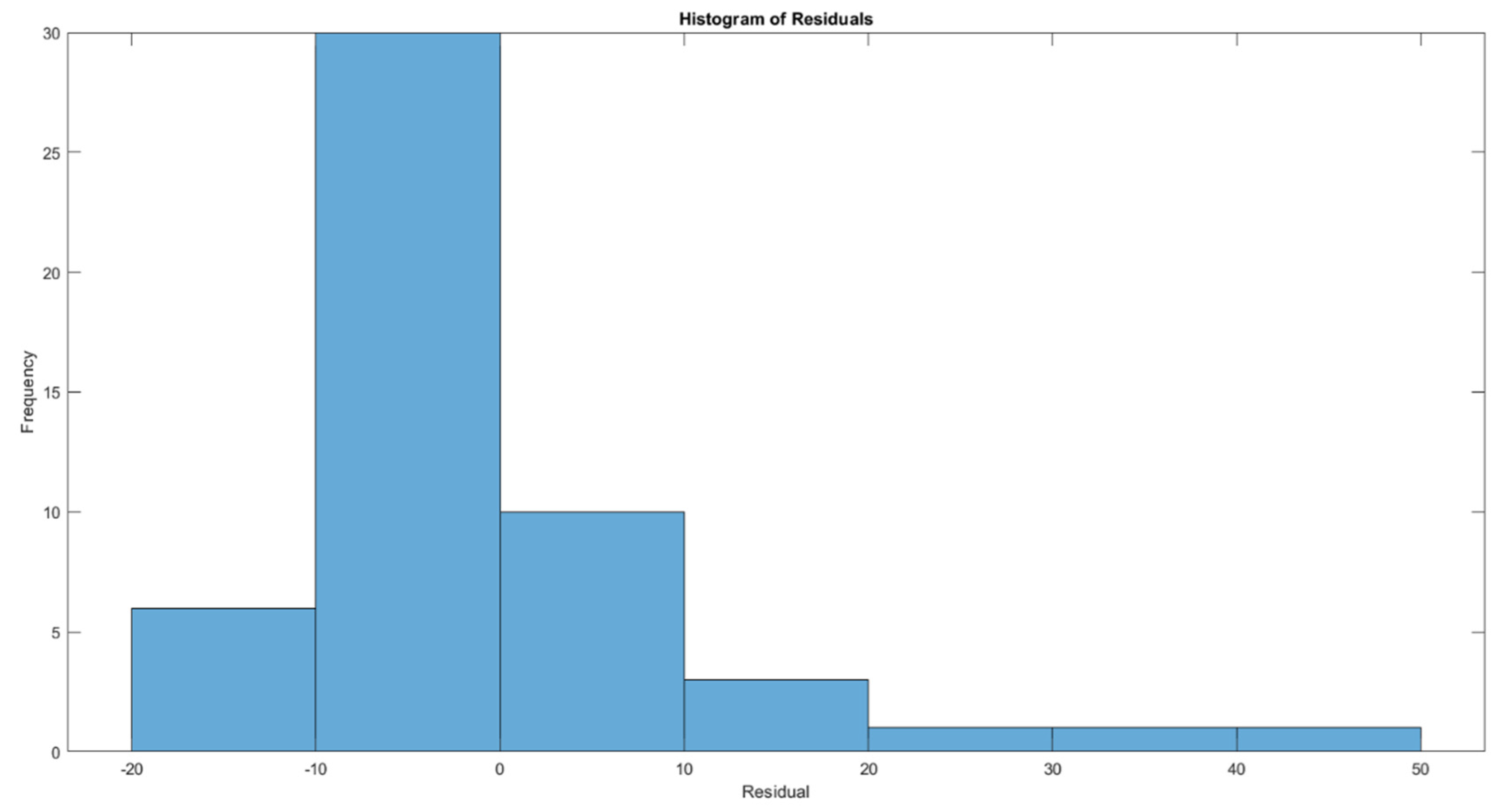
The histogram of residuals from Figure 9 provides a distribution of the errors between the predicted and actual values from the Random Forest model, aimed at predicting PM2.5 levels. The residuals are skewed to the right, indicating that the model tends to underpredict PM2.5 levels more frequently than overpredict. Most residuals cluster around 0, suggesting that the model's predictions are generally accurate, but there are notable instances where the model predictions deviate significantly from the actual values, as seen in the long tail towards higher positive values. This skewness and the presence of large residuals could imply that while the model is effective for typical scenarios, it struggles with accurately predicting higher levels of PM2.5, possibly during unusual pollution events or under specific environmental conditions not well-represented in the training data. Addressing this might require refining the model further, perhaps by incorporating more data points under extreme conditions or adjusting the model's sensitivity to outliers.
8. Conclusions
This study leveraged advanced machine learning techniques to predict PM2.5 levels at the University of Petroșani campus, emphasizing the critical role of air quality in environmental health and academic settings. By integrating local and regional data sources, including real-time IoT sensor readings and historical pollution data, we developed a comprehensive model that improves our understanding and ability to forecast air quality dynamics effectively.
Our findings underscore the significant influence of specific pollutants, notably nitrogen oxides (NO and NO2), ozone (O3), and carbon monoxide (CO), on PM2.5 concentrations. The Random Forest model, which demonstrated the highest predictive accuracy with an R2 score of 0.82764, highlighted the importance of these pollutants in predicting PM2.5 levels. Notably, NO emerged as the most influential predictor, suggesting vehicular and industrial emissions as major contributors to particulate matter levels in the area. This insight is particularly valuable, providing a targeted avenue for mitigation strategies focused on reducing emissions from these sources.
From a practical standpoint, this research provides a robust framework for air quality management at the University of Petroșani and can be adapted to similar environments with unique air quality challenges.
The novelty of the research lies in the integration of advanced machine learning techniques, particularly ensemble method like Random Forest, combined with real-time data collection from IoT sensors for predicting PM2.5 levels. This approach allows for a more dynamic and precise modeling of air quality influenced by a mix of pollutants, relative humidity, and temperature. The innovative aspect is not just the prediction of PM2.5 itself but the detailed examination of how various pollutants and environmental factors interact and influence these predictions, tailored to a specific setting like a university campus. This methodology extends beyond traditional static models by incorporating real-time environmental data and leveraging complex machine learning frameworks to enhance prediction accuracy and responsiveness to changes in air quality.
The approach of using machine learning to predict PM2.5 levels, compared to direct measurement with sensors, offers several advantages. Firstly, predictive modeling can provide insights before actual high pollution events occur, allowing for preemptive actions to mitigate adverse effects. This is particularly beneficial in urban planning and public health advisories. Additionally, machine learning models can integrate a variety of data sources including historical data, real-time IoT sensor data, weather conditions, and pollutant levels, making the predictions more comprehensive and accurate. This method also helps in understanding complex interactions between multiple variables, which is often challenging with direct measurements alone. Furthermore, predictive models can be cost-effective by reducing the need for extensive sensor networks, especially over large areas or in resource-limited settings.
To date, specific research focused on developing PM2.5 prediction models exclusively within university campus settings using machine learning approaches is not prominent in the literature. Most studies explore broader urban environments or apply their findings generally across multiple settings, including educational facilities. However, such studies do not explicitly center on university campuses as unique entities with distinct environmental dynamics and challenges. This highlights a significant research gap, emphasizing the need for targeted predictive models that cater to the specific conditions of university campuses that has been addressed by the present research. These models would be invaluable for effectively managing campus-specific air quality issues, potentially improving health and environmental conditions in these micro-environments.
One notable limitation of our research is the potential for model bias due to the finite scope and heterogeneity of the dataset used, which primarily focuses on the University of Petroșani and its immediate environment. While the model incorporates a range of pollutants and meteorological factors, the exclusion of other influential variables such as finer-scale traffic data, industrial emissions specifics, and broader geographical environmental factors might limit the comprehensiveness of the predictions. Additionally, the use of machine learning models, particularly those reliant on large amounts of historical data, introduces the risk of overfitting, especially when applied to predict conditions under atypical circumstances not well-represented in the training data. The reliance on historical data also assumes that past conditions accurately predict future states, which may not account for sudden changes in emission patterns or meteorological conditions. These limitations highlight the need for continuous model updating and validation against real-time data to ensure the accuracy and relevance of the predictive outcomes in changing environmental conditions.
To enhance the predictive capabilities and robustness of air quality models, future research should aim to integrate a broader spectrum of environmental and temporal data, particularly focusing on dynamic factors that significantly impact pollutant behavior. Incorporating additional variables such as wind speed, humidity levels beyond relative humidity, and atmospheric pressure could significantly refine the accuracy of PM2.5 predictions. These meteorological factors play crucial roles in the dispersion and concentration of airborne pollutants and can provide deeper insights into the daily and seasonal variability of air quality. Additionally, integrating traffic data, especially in urban or semi-urban settings like university campuses, could help correlate vehicular emissions directly with observed pollution levels, offering a more nuanced understanding of primary pollution sources.
Moreover, advancing the methodological approach by incorporating time-series analysis would leverage the temporal data to uncover trends, seasonal patterns, and cyclical behaviors of pollutants. This approach could transform reactive air quality management into a more proactive strategy, enabling the prediction of pollution peaks and troughs which is vital for effective planning and intervention. Employing sophisticated machine learning techniques that adeptly handle non-linear relationships—such as advanced ensemble methods or deep learning models—could further enhance model performance. Ensuring robust model validation through comprehensive cross-validation techniques will also be crucial. This process, involving the iterative training and testing of the model on various data subsets, helps in safeguarding against overfitting, thereby enhancing the model's generalizability and reliability across different environmental conditions and geographical settings. Such enhancements not only promise to elevate the precision of air quality forecasting but also bolster the overall utility of predictive models in public health and environmental policy frameworks.
Author Contributions
Conceptualization, A.I., M.L. and F.A.P.; methodology, A.I.; software, M.L. and M.W.; validation, C.R., F.A.P. and M.W.; formal analysis, M.L.; investigation, C.R.; resources, A.I. and M.L.; data curation, F.A.P. and M.W.; writing—original draft preparation, A.I. and M.L.; writing—review and editing, C.R.; visualization, M.L.; supervision, A.I.; project administration, M.L.; funding acquisition, F.A.P. All authors have read and agreed to the published version of the manuscript.
Conflicts of Interest
The authors declare no conflicts of interest.
References
- University of Cambridge. Cambridge Green Challenge. Available online: https://www.msm.cam.ac.uk/cambridge-green-challenge (accessed on 3 July 2024).
- University of Leeds. Living Lab for Air Quality. Available online: https://sustainability.leeds.ac.uk/the-living-lab/airquality/(accessed on 3 July 2024).
- Just Transition. Available online: https://theclimatevertical.com/just-transition-in-valea-jiului/(accessed on 3 July 2024).
- IQAir air quality monitoring platform. Available online: https://www.iqair.com/romania/hunedoara/petrosani (accessed on 15 July 2024).
- Tang, D., Zhan, Y., & Yang, F. (2024). A review of machine learning for modeling air quality: Overlooked but important issues. Atmospheric Research, 107261. [CrossRef]
- Zhang, Z., Zhang, S., Chen, C., & Yuan, J. (2024). A systematic survey of air quality prediction based on deep learning. Alexandria Engineering Journal, 93, 128-141. [CrossRef]
- Meena, K. K., Bairwa, D., & Agarwal, A. (2024). A machine learning approach for unraveling the influence of air quality awareness on travel behavior. Decision Analytics Journal, 11, 100459.
- Liu, Q., Cui, B., & Liu, Z. (2024). Air Quality Class Prediction Using Machine Learning Methods Based on Monitoring Data and Secondary Modeling. Atmosphere, 15(5), 553. [CrossRef]
- Dey, P., Dev, S., & Phelan, B. S. (2024). Predicting Multivariate Air Pollution: A Gaussian-Mixture Nested Factorial Variational Autoencoder Approach. IEEE Geoscience and Remote Sensing Letters. [CrossRef]
- Ansari, M., & Alam, M. (2024). An intelligent IoT-cloud-based air pollution forecasting model using univariate time-series analysis. Arabian Journal for Science and Engineering, 49(3), 3135-3162.
- Aram, S. A., Nketiah, E. A., Saalidong, B. M., Wang, H., Afitiri, A. R., Akoto, A. B., & Lartey, P. O. (2024). Machine learning-based prediction of air quality index and air quality grade: a comparative analysis. International Journal of Environmental Science and Technology, 21(2), 1345-1360. [CrossRef]
- Mishra, A., & Gupta, Y. (2024). Comparative analysis of Air Quality Index prediction using deep learning algorithms. Spatial Information Research, 32(1), 63-72. [CrossRef]
- Essamlali, I., Nhaila, H., & El Khaili, M. (2024). Supervised Machine Learning Approaches for Predicting Key Pollutants and for the Sustainable Enhancement of Urban Air Quality: A Systematic Review. Sustainability, 16(3), 976. [CrossRef]
- Shoukry, F., Raafat, R., Tarabieh, K., & Goubran, S. (2024). Indoor Air Quality and Ventilation Energy in University Classrooms: Simplified Model to Predict Trade-Offs and Synergies. Sustainability, 16(7), 2719. [CrossRef]
- Peng, H. (2015). Air quality prediction by machine learning methods (Doctoral dissertation, University of British Columbia).
- Yang, Y., Zheng, Z., Bian, K., Song, L., & Han, Z. (2017). Real-time profiling of fine-grained air quality index distribution using UAV sensing. IEEE Internet of Things Journal, 5(1), 186-198. [CrossRef]
- Tiwari, A.; Aljoufie, M. Modeling Spatial Distribution and Determinant of PM2.5 at Micro-Level Using Geographically Weighted Regression (GWR) to Inform Sustainable Mobility Policies in Campus Based on Evidence from King Abdulaziz University, Jeddah, Saudi Arabia. Sustainability 2021, 13, 12043. https://doi.org/10.3390/su132112043. [CrossRef]
- Gaman, A. N., Simion, A., & Simion, S. (2024). Air quality monitoring in the eastern Jiul Valley. In MATEC Web of Conferences (Vol. 389, p. 00044). EDP Sciences. [CrossRef]
Figure 1.
Research methodology.
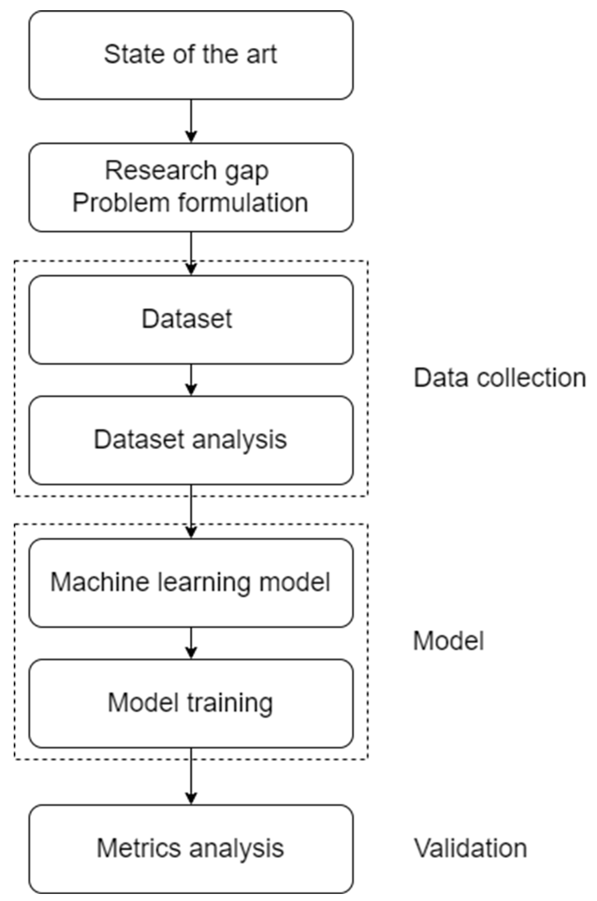
Figure 2.
Boxplot for input variables.
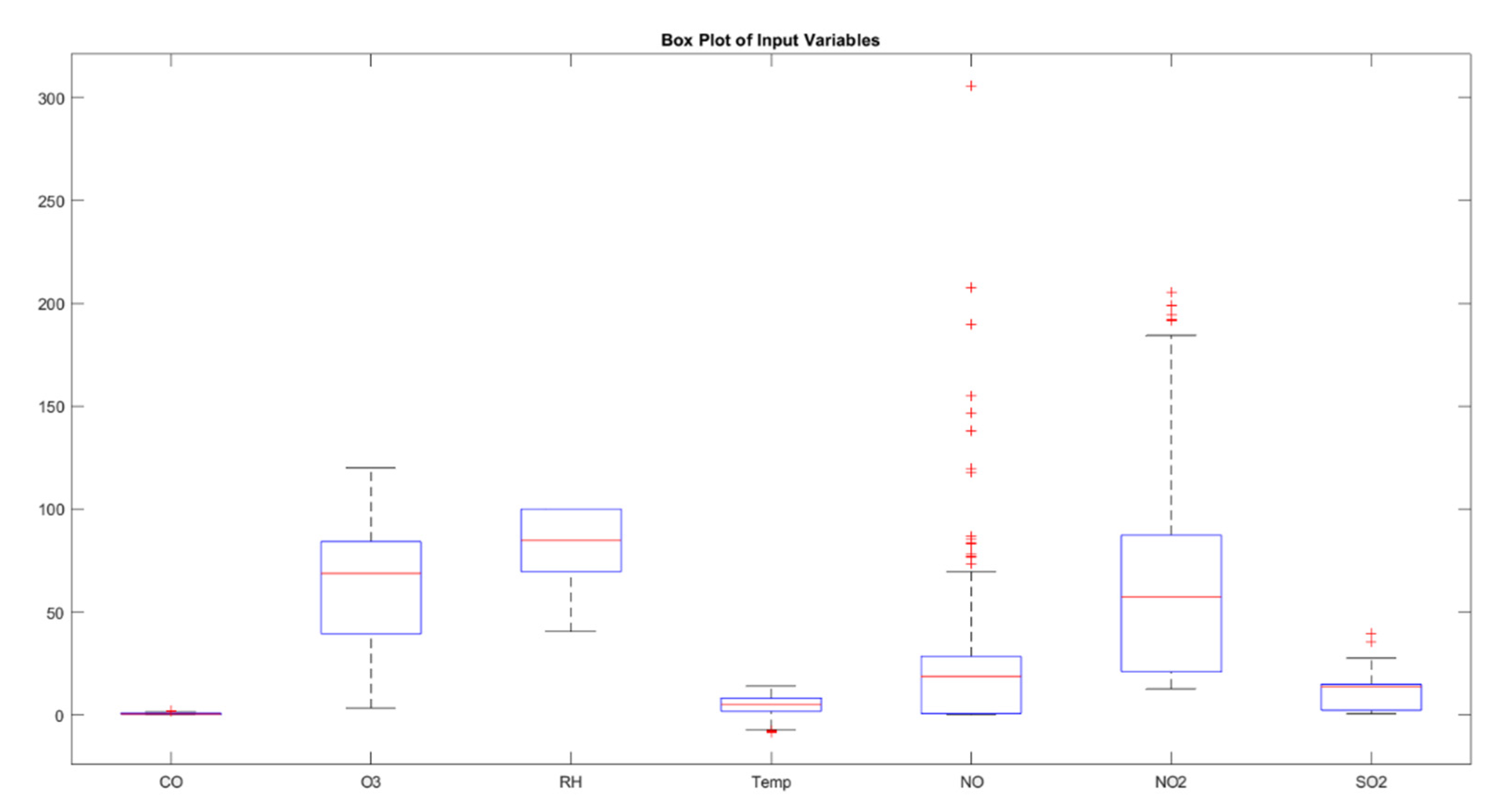
Figure 3.
Variables histograms.
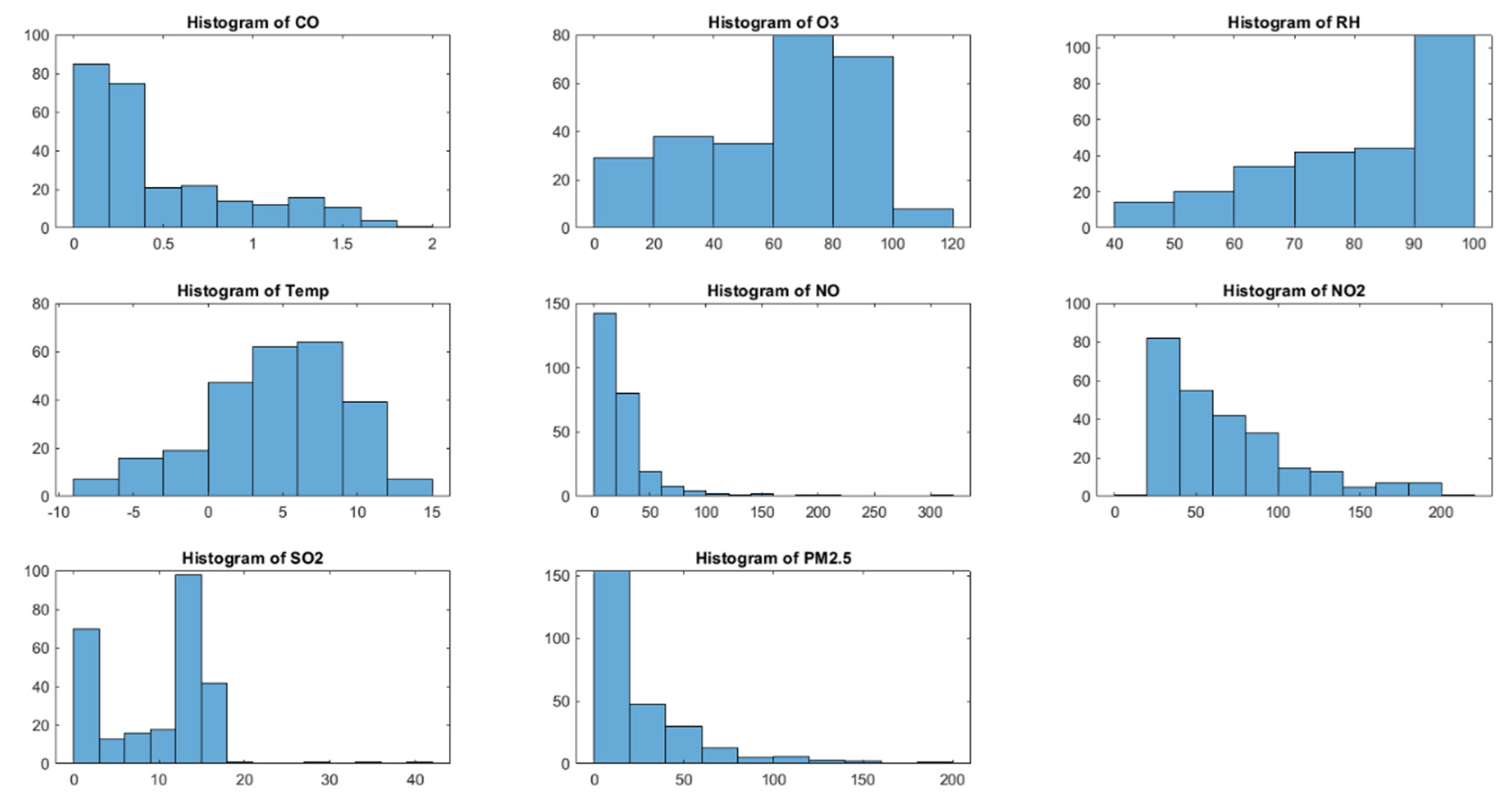
Figure 4.
Correlation matrix.
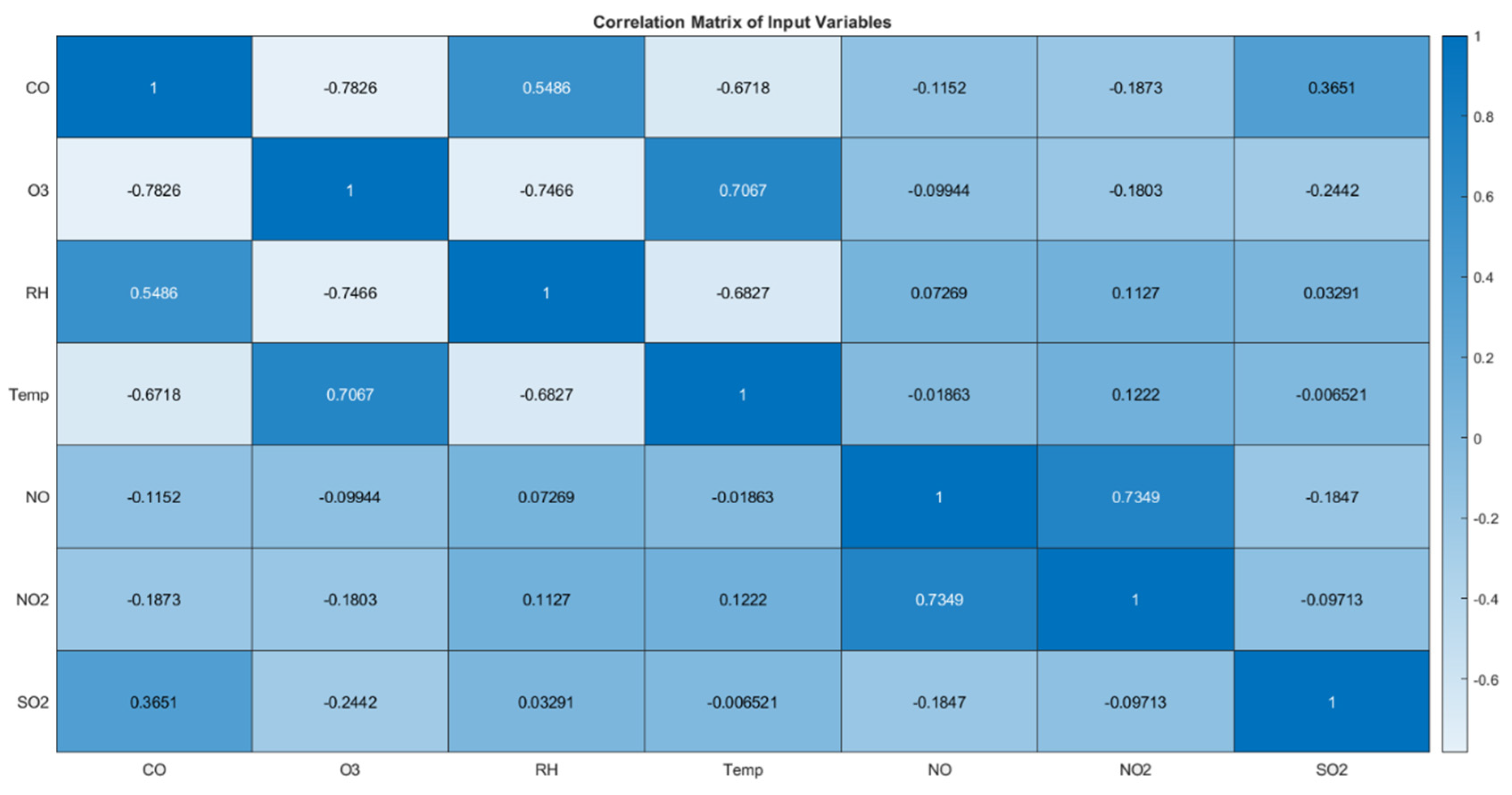
Figure 5.
Output correlations.
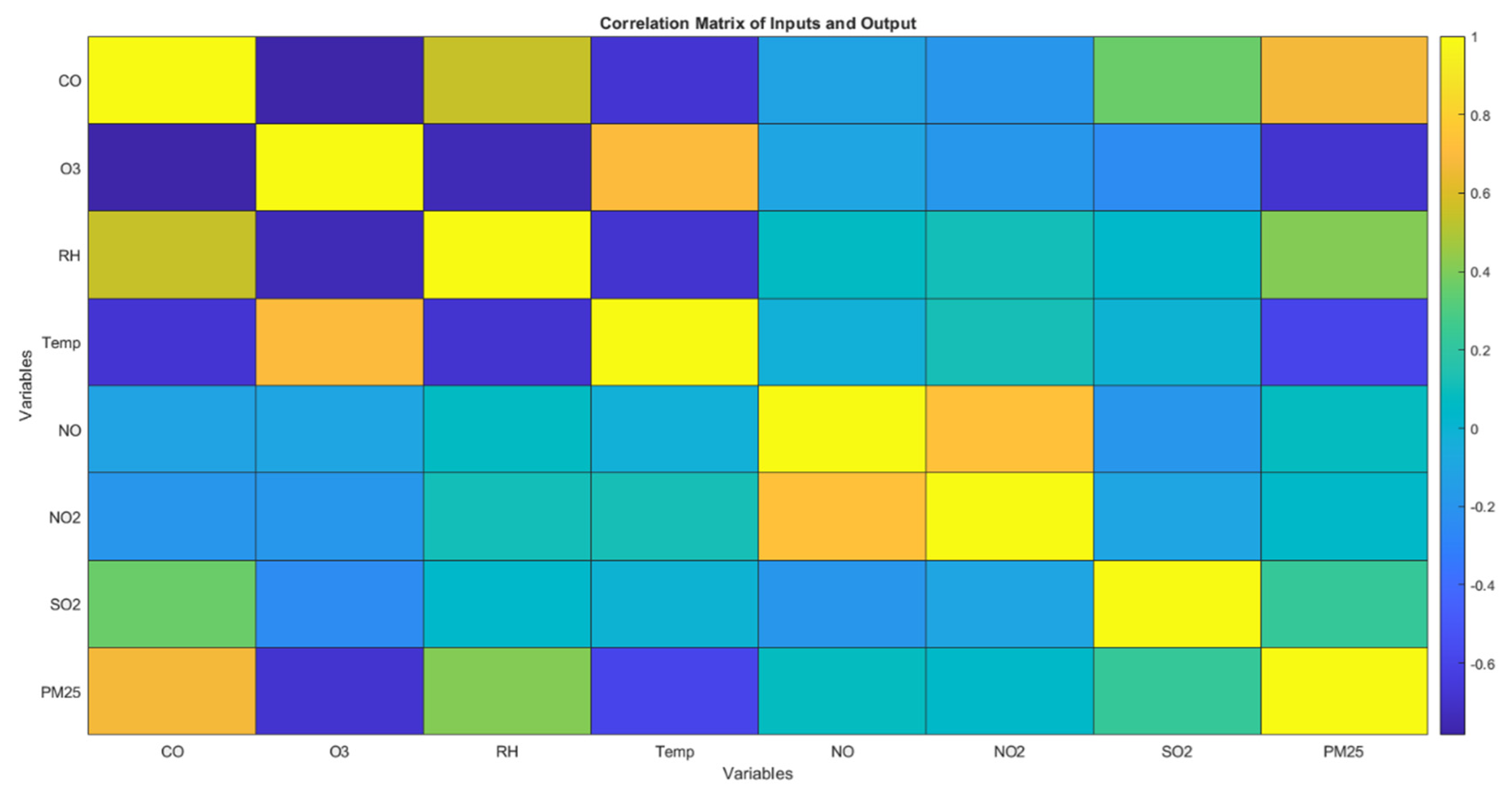
Figure 6.
R2 comparison for different models.
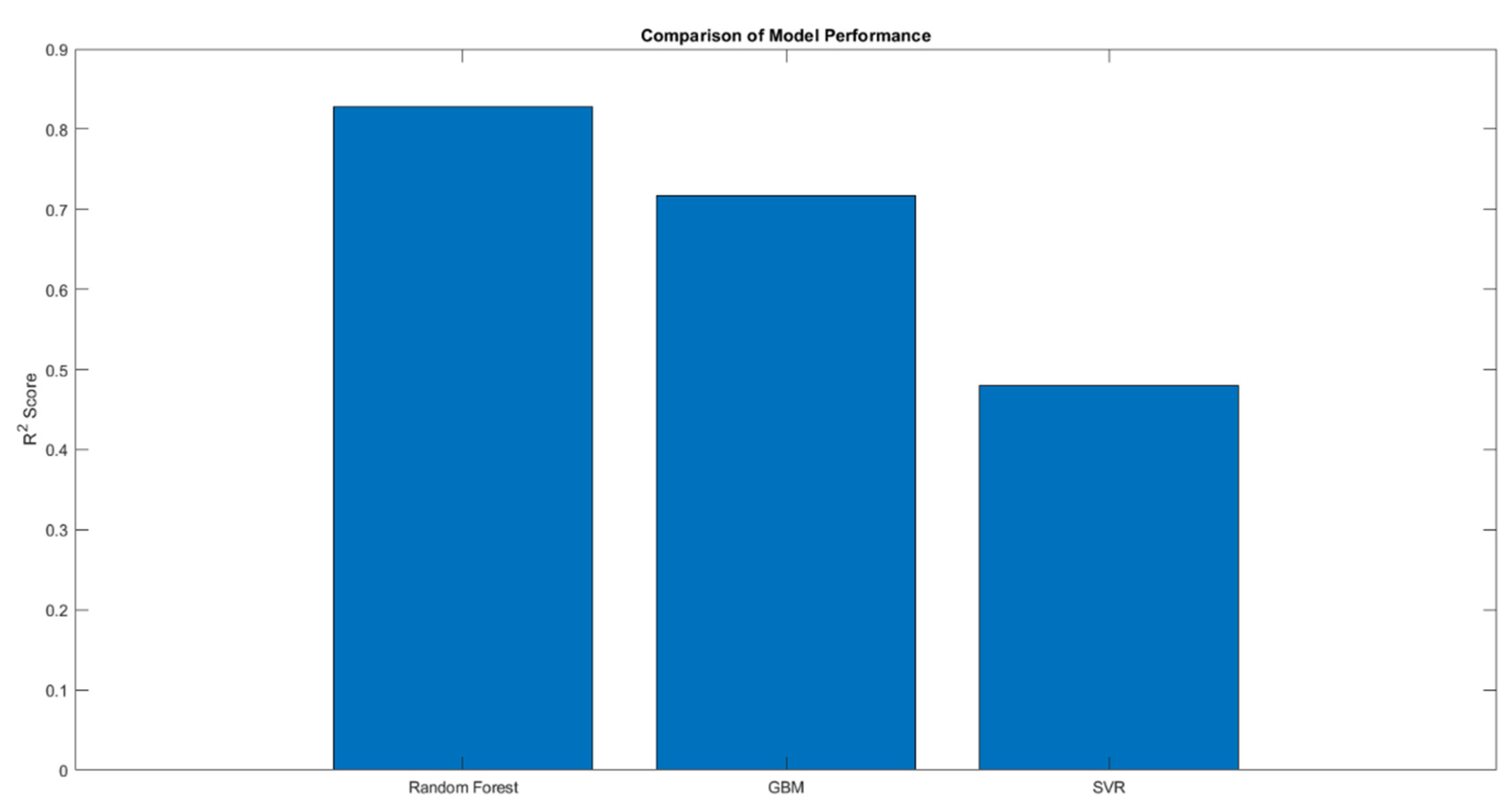
Figure 7.
Feature importance.
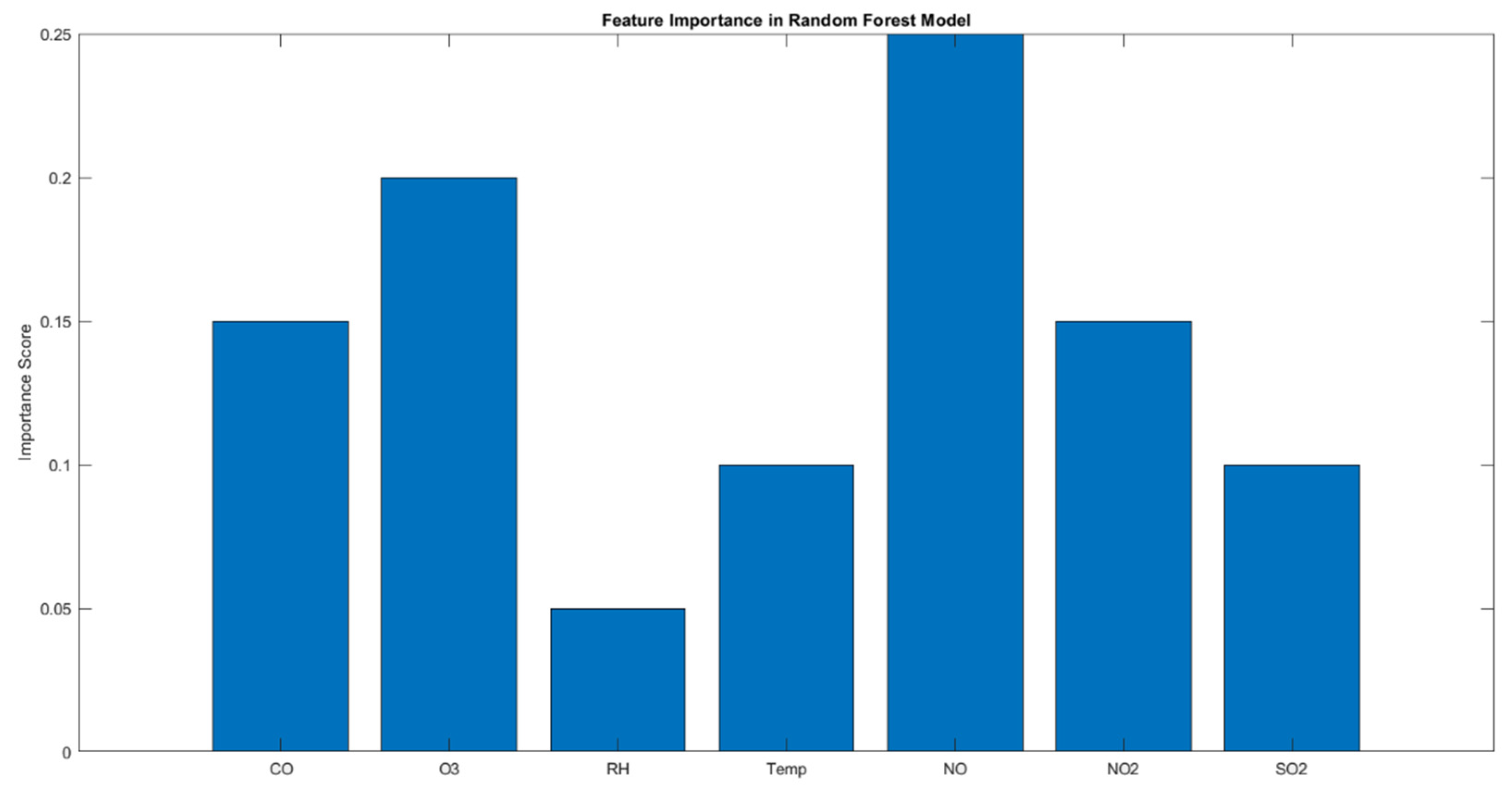
Figure 8.
Parameter impact.
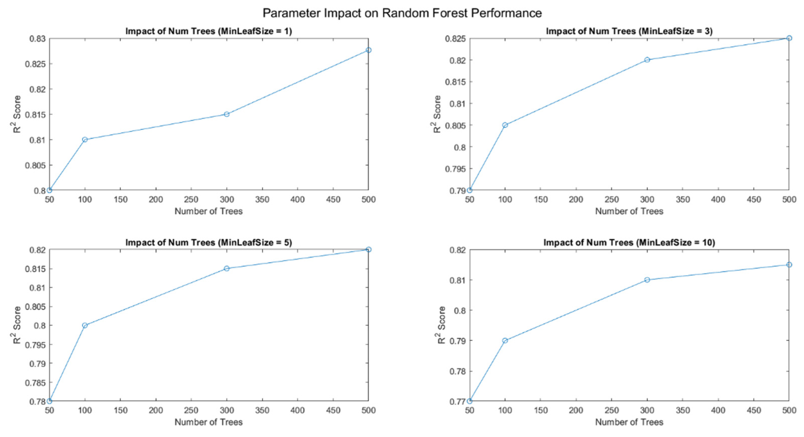
Figure 9.
Histogram of residuals.
Disclaimer/Publisher’s Note: The statements, opinions and data contained in all publications are solely those of the individual author(s) and contributor(s) and not of MDPI and/or the editor(s). MDPI and/or the editor(s) disclaim responsibility for any injury to people or property resulting from any ideas, methods, instructions or products referred to in the content. |
© 2024 by the authors. Licensee MDPI, Basel, Switzerland. This article is an open access article distributed under the terms and conditions of the Creative Commons Attribution (CC BY) license (http://creativecommons.org/licenses/by/4.0/).
Copyright: This open access article is published under a Creative Commons CC BY 4.0 license, which permit the free download, distribution, and reuse, provided that the author and preprint are cited in any reuse.


