
Submitted:
06 December 2024
Posted:
10 December 2024
You are already at the latest version
Abstract
This study aims to determine the optimal frequency for monitoring airborne pollutants in densely populated urban areas to effectively capture their temporal variations. While environmental organizations worldwide typically update air quality data hourly, there is no global consensus on the ideal monitoring frequency to adequately resolve pollutant (Particulate Matter) time series. By applying temporal variogram analysis to particulate matter (PM) data over time, we identified specific measurement intervals that accurately reflect fluctuations in pollution levels. Using January 2023 air quality data from the Joppa neighborhood of Dallas, TX, Temporal Variogram analysis was conducted on three distinct days with varying PM2.5 pollution levels. For the most polluted day, the optimal sampling interval for PM2.5 was determined to be 12.25 seconds. This analysis shows that highly polluted days are associated with shorter sampling intervals, highlighting the need for highly granular observations to accurately capture variations in PM levels. Using the variogram analysis results from the most polluted day, we trained Machine Learning models that can predict the sampling time using meteorological parameters. Feature importance analysis revealed that humidity, temperature and wind speed could significantly impact the measurement time for PM2.5. The study also extends to the other size fractions measured by the air quality monitor. Our findings highlight how local conditions influence the frequency required to reliably track changes in air quality.
Keywords:
Environmental Research
; Particulate Matter
; Air Quality
; Statistics
; IOT
; Variogram
; Optimization
; Data Science
; Machine Learning
; Big Data
; Sensors
1. Introduction
The objective of this study is to determine the optimal sampling frequency for various PM size fractions and to assess the influence that meteorological parameters have on the required sampling frequency. The study focuses on the temporal fluctuations of airborne particle content [1,2,3,4,5,6,7] within a specific neighborhood. Due to the typical Environmental Agencies’ practice of reporting airborne particulate concentration just once every hour, short-duration large exposures easily go unresolved with a temporal measurement resolution of an hour. Moment-to-moment fluctuations in airborne particulate concentrations are influenced by a complex interplay of factors. Variations in the sources of particulates [8,9,10], such as emissions from vehicles, industrial activities, construction sites, and natural phenomena such as wildfires and volcanic eruptions, play an important role. These fluctuations are further compounded by changing meteorological conditions, including wind patterns, temperature, atmospheric pressure, and humidity, which affect how particulates spread or dilute. In addition, airborne particulates can undergo chemical reactions, transforming in composition and concentration. Physical processes such as deposition and resuspension [11] also contribute to variability, as particles settle out of the air or are stirred back into the air. Human activities, with their variable nature, significantly affect particulate levels through changes in traffic flow, industrial output, and construction activities. Furthermore, local terrain, such as the presence of valleys, street canyons, or other urban structures, can influence the dispersion and concentration of particles. All of these factors together result in the observed fluctuations in airborne particulate matter over short time periods.
Variograms are useful for objectively characterizing the appropriate frequency at which to make air quality observations. The range parameter of the variogram is used to determine the temporal fluctuation of the PM concentration. These fluctuations are computed daily, weekly, monthly, and even yearly. In the latter part of the study, we will consider the impact of the meteorological parameters on the sampling time for the most polluted day. For our preliminary investigation, we examine three specific days in January 2023 that have different degrees of pollution.
2. Materials and Methods
2.1. Sensors Overview
Environmental agencies report the concentration of airborne particles every hour, which means that changes in PM concentrations on shorter time scales will not be captured. So, we use the Central Node, which is a powered stationary sensor system. This monitor was designed by Dr. Lakitha Wijeratne of the MINTS lab at UT Dallas. MINTS stands for the Multiscale Integrated Sensing and Simulation Lab that works in developing intelligent sensing systems. The Central Node is one of these sensing systems. It is a 24/7 distributed sentinel that monitors and posts environmental data frequently and consistently. This node is equipped with an array of sensor systems designed to monitor various environmental parameters, including PM levels recorded every second throughout the day.
This research focuses specifically on the IPS7100, BME280, and AirMar sensors within the MINTS Central Node [12,13,14]. Using the variogram model, our aim is to determine the optimal sampling interval for each PM size fraction measured by the IPS7100. Meteorological parameters play a critical role in influencing ambient PM concentrations, as demonstrated in numerous studies [15,16,17,18] showing how these parameters affect PM formation, dispersion, and removal. Consequently, we incorporate climate data from the BME280 and AirMar sensors to analyze the relationship between PM sampling intervals and meteorological conditions.
The data for this study are sourced from the Central Node located in the Joppa neighborhood of the Dallas-Fort Worth Metroplex, a region heavily impacted by industrial encroachment and severe pollution.
The following are the sensors from the Central Node Air module that were utilized for this research work:
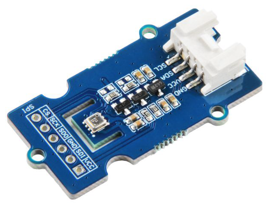
2.1.1. IPS7100
Intelligent Particle Sensor (IPS) [19] is an optical counter which detects particulate matter size fractions ranging from to . It outputs both the particle count and the concentration for each size fraction. It separates the data into 7 bins, one for each size fraction. So we have 14 values as the output. The IPS7100 monitors common size fractions for air quality, such as ( includes all particles with an aerodynamic diameter m, with similar definitions applied to other size fractions), , and . In addition, it measures size fractions such as , , , and . It is compatible with the UART and C protocols. In our design, we make use of the C protocol. The IPS sensor can run at 65 mA and 5V, making it ideal for low-power applications. The Central Node air module detects the PM concentration and counts with a high granularity of 1 second. Hence, this data are suitable to resolve the time series.
Figure 1.
IPS7100.

2.1.2. BME280
The Bosch BME280 sensor [20] measures the climate data (temperature, pressure, and humidity, respectively). It operates on a voltage range of 1.71 V to 3.6 V. It supports the C and SPI protocols. In our design, we employ the C protocol. The temperature, pressure, and humidity data are collected at a granularity of 10 seconds. BME280 provides a quick response rate with accuracy and resolution, while keeping noise at a minimum.
Figure 2.
BME280.
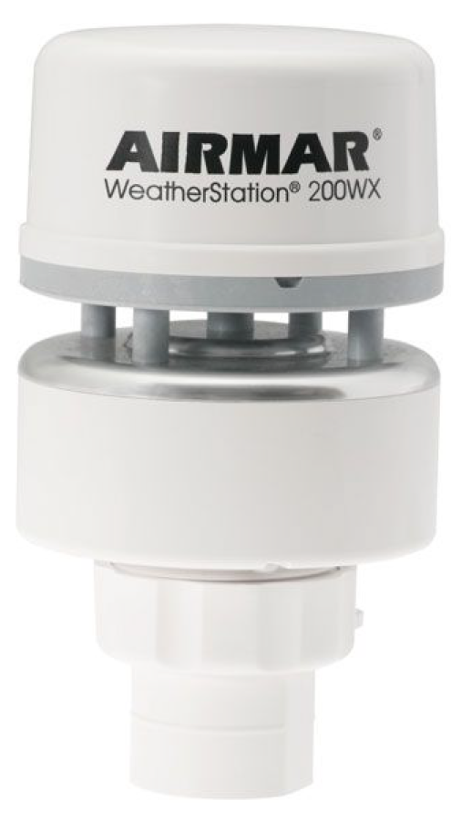
2.1.3. AirMar Weather Station
The AirMar Weather Station [21] is a reference sensor designed to measure a range of parameters including air temperature, barometric pressure, relative humidity, wind speed, etc. It uses ultrasonic technology for wind measurement. Hence, improving accuracy without the need for moving parts. We collect the wind speed data every 10 seconds.
Figure 3.
AirMar Weather Station.
2.2. Data Collection
The data collected for this study span from January 1 2023, 06:00:00 UTC, to February 1, 2023, 05:59:59 UTC, and include measurements from the IPS7100, BME280 and AirMar sensors. The time stamp of the data collected is in UTC, and it will be later converted to the designated local time zone. The data for each sensor are collected as daily CSV files and later processed.
The PM data was captured at a fast sampling rate of 1 second for IPS7100. The 10 second interval for the meteorological sensors (BME 280 and AirMar) was specifically chosen to prevent latency issues that could arise from having multiple sensors communicating on the same bus to guarantee efficient data collection.
The sensors used in the study are prone to measurement errors. So the data collected for this study will be checked based on the measurement range for each sensor. Table 1 below provides details of the sensors, including their parameters, units, measurement ranges, and resolution/frequency of measurements.
2.3. Variogram Analysis
2.3.1. Temporal Variogram Equation
Based on the variogram analysis [22,23,24,25,26,27,28,29,30,31] of the collected PM data, we can characterize the frequency with which airborne particulate observations should be made to adequately resolve the PM time series. We utilize Semi-Variograms (also known as Variograms), a Geo-Statistical model that calculates the autocovariance of the points in a sample. This method is used to identify the temporal fluctuations that occurred over a period of 24 hours. We do the analysis for each of three distinctly polluted days separately. This allows us to better understand how the sampling period for each of the PM size fractions change over time.
The variogram is calculated as the average squared difference between points separated by a specific distance (time lag). The semivariogram is half of the variogram, though the terms are often used interchangeably. The equation for a general temporal semivariogram for the PM data takes the form
: represents the Semi-Variogram as a function of time lag.
N: represents the total number of data point pairs for which the Variogram is constructed.
: the PM Concentration measured for time,
: the PM Concentration measured before or after a time lag of from the time.
2.3.2. Key Elements of a Variogram
The Nugget, Sill, and Range are the three primary elements that make up a variogram. The Nugget is the y-intercept of the semi-variogram vs lag time plot. It can also be defined as the value of the variogram, , as approaches 0. Ideally, when there are two simultaneous PM observations, they should have the same value. This would result in a nugget value of zero. However, in reality, this is often not the case. Measurement errors inherent to the sensor during sampling or temporal variations of PM at time gaps smaller than the sampling intervals introduce some randomness. This randomness causes slight differences between values that would otherwise be identical. As a result, the nugget is non-zero. This phenomenon is known as the Nugget Effect [32].
The Sill is the point on the y-axis of the semi-variogram vs lag time plot, where the variogram starts to level off to a near-constant value. The leveling indicates that beyond that lag distance or time lag , the points become uncorrelated.
The Range is the distance beyond which the Variogram flattens out. Here, it is used to identify the temporal scale beyond which the data is no longer correlated. To obtain it, we find the x coordinate on the semi-variogram vs lag time plot that corresponds to 95% of the sill.
Among the attributes described above, range is of particular interest. When determining the range for each time step, sliding windows are an effective tool to use. For each time step and for a sliding window of specific size, we find the temporal scale beyond which the correlation between measurements diminishes. To determine the range of our variograms, we first fit an empirical variogram to a theoretical model. We then identify the point on this theoretical variogram curve where the correlation effectively reaches zero (or plateaus). The x-coordinate corresponding to this point is defined as the Range of the variogram.
Here, the Theoretical Variogram model used for fitting is an exponential model. Exponential Variogram’s [33] have been useful in capturing high variability which is commonly seen in PM data due to localized sources of pollution. It follows the equation:
where is the semivariance in the lag time . is the Nugget. C is the Sill minus the Nugget. a is the Range. h is the lag time (in our case it varies from 0 to 5 minutes).
The model accuracy can be found using the Mean Squared Error (MSE) which is the averaged squared difference between the actual value and the predicted value. The lower the MSE, the better the model will be, indicating smaller errors. The MSE is given by:
The goodness of fit of the empirical variogram with theoretical model, can also be assessed using the Coefficient of Determination (). This helps in estimating the model performance. The value can range from 0 to 1, with values closer to 1 indicating a better fit. The score is calculated as:
- is the Residual Sum of Squares (RSS),
- is the Total Sum of Squares (TSS),
- represents the Empirical value,
- represents the Theoretical value,
- is the mean of all Empirical values.
2.3.3. Rolling Temporal Variogram
To determine the variability of the PM measurement time throughout the day at a high granularity, we calculate the Range for each 1 second time step. To do that, we use sliding windows of 15 minutes and a time lag of 5 minutes. Starting from the first second of the day, we create a rolling temporal variogram using the equation:
The above equation employs a 15 minute sliding window that traverses the entire day, week, month, or year of the data at a time step of 1 second. The goal here is to obtain a range value for the shortest resolution possible. Here i is the variable that defines the width of the window (15 x 60s = 900s). j is the variable that decides the duration for which the window must traverse. It helps in generating the moving variogram. It starts off at 1 s and allows our algorithm to generate variograms over each pair of points in time that are 900 seconds apart (e.g. (1, 901), (2, 902), (3, 903), and so on). N is the total number of pairs of concentrations of PM across which the variogram is constructed. M represents the first value of the last sliding window. This will be equal to the time duration for which PM levels are measured minus the width of one sliding window (15 minutes). For a day’s data, it will be equivalent to
used in our study is 5 minutes. is the PM data measured for time. is the PM data measured after a time delay of from the time (because we are considering a forward traversing rolling temporal variogram).
2.4. Machine Learning Setup
The temporal variogram is applied to obtain the measurement time for all PM concentrations (from to ) for the month of January 2023. After estimating the PM measurement time for each size fraction, we proceed to assess the impact of various meteorological parameters on this measurement time. For this part of the study, we used parameters such as Temperature, Atmospheric Pressure (referred to as Pressure), Humidity, and Wind Speed, all of which were recorded by the Central Node. Nonlinear and nonparametric regression models were used to estimate the measurement time for each size fraction [34,35,36], using meteorological parameters as input. Wind speed, humidity, temperature, and pressure data from the Central Node were recorded at 10-second intervals. The estimated measurement time for each size fraction is considered as the target variable. We will develop seven models corresponding to each of the seven size fractions, using measurement time as the target variable and meteorological parameters as predictors.
For modeling purposes, we use ensemble learning methods like Random Forest [37]. Random forests are often known for their versatility and flexibility. It is widely used in air quality monitoring because they are good at handling high-dimensional data and are robust to noise. They also produce accurate and interpretable results. Random forests use decision trees, also known as Classification And Regression Trees (CART), as their base learners. Individual decision trees are prone to over-fitting as they may create individual leaf nodes for each observation. In Random Forest, each tree is fitted using a bootstrapped sample from the original data, and the results are averaged later. This approach is known as Bagging. Random forests also use random subsets of features to split each tree, preventing important features from appearing at the top of each decision tree. This reduces the overfitting and the correlation between trees.
The best Random Forest Regression model will be chosen after hyperparameter [38,39] optimization through Random Search CV. Random Search CV combines Random Search and Cross Validation. Instead of testing all possible values for each hyperparameter, it randomly chooses a subset of combination to evaluate. This approach is useful when multiple hyperparameters are involved. The cross validation part in Random Search CV helps in getting a generalized model. In cross-validation, we divide the entire data set into multiple folds. In each round, one fold is used for validation and the other folds are used for training. This process is repeated for each fold, and the results are averaged to obtain a reliable estimate of the model’s performance. The model with the best (or lowest MSE) value is chosen for the test. This helps in model performance when it comes to unseen data.
The feature importance ranking in Random Forest is a key aspect which helps us determine which features contribute the most to the model’s goodness-of-fit. Random Forest ranks its features based on average decrease in variance for regression when a feature is used to split the data. However, this becomes an issue when features are highly correlated, as Random Forest tends to distribute importance across these correlated features. Hence, we choose a model-agnostic feature ranking method such as permutation ranking [40,41]. Here, the performance of the model ( or MSE) is first calculated on the original data set. Now, for each feature, the values are randomly shuffled among that feature while keeping the other features and target value as is. The model performance is then evaluated using the shuffled feature. If there is a large performance drop, it shows that the feature is very important, while a small drop indicates that the feature is less relevant. If features are correlated to each other, then shuffling them will result in a smaller dip. This can help the model to rely on other correlated features to capture similar information.
3. Results
3.1. Preliminary Analysis
The raw data collected was consolidated into a single data set for each sensor. For each data set, the time stamp was converted to Central Time to align with the local timezone. Duplicate timestamps were identified and consolidated by averaging the values. Rows containing missing or NA values were removed to ensure data consistency. Invalid numerical values, such as any string-numerical columns in the dataset, were converted to numerical format. To maintain temporal consistency, the gaps in the timestamps (1-second intervals for the IPS7100 and 10-second intervals for the meteorological sensors) were imputed using forward and backward imputation methods. The cleaned data sets were then verified to ensure that they contained the correct number of records per day - 86,400 records per day for the IPS7100 and 8,640 records per day for the BME280 and AirMar sensors. Finally, the cleaned data were stored as CSV files, with timestamps and categorization based on the relevant sensor, ready for analysis.
For the initial analysis, we will compare the PM concentration levels for each day in January 2023. This analysis utilizes the calendar plot functionality provided by the openair package in R, a comprehensive toolkit designed to analyze air quality and atmospheric data. The calendar plot function effectively visualizes Joppa PM data by displaying daily average concentrations in a clear and intuitive calendar format, making it easier to identify patterns and trends throughout the month. For ease of explaining the model in the upcoming section, we will focus specifically on the calendar plots for concentration.
The calendar plot below shows the daily average Concentration of Joppa for January 2023.
Figure 4.
Variation of Daily Average Concentration Across January 2023.
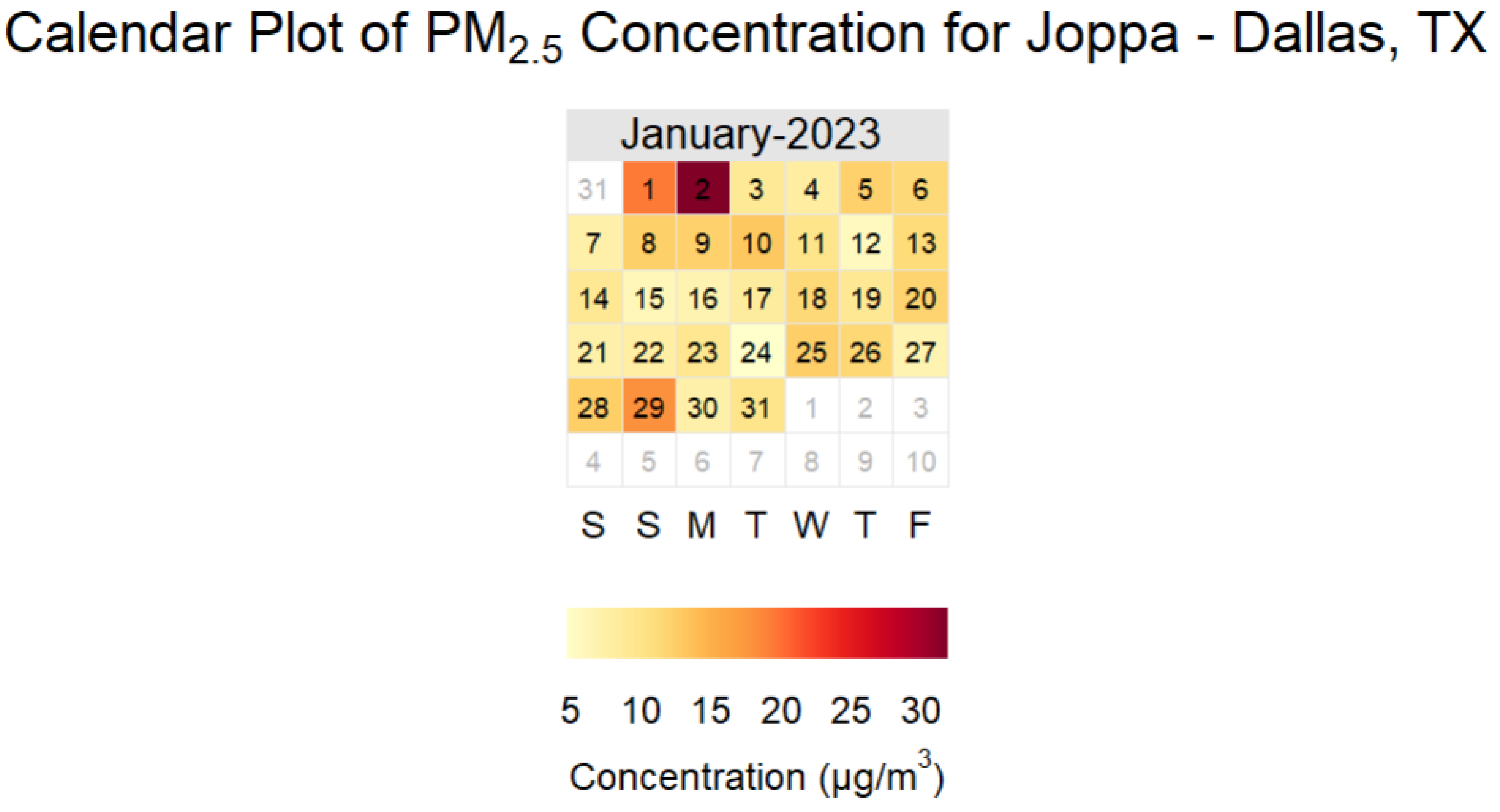
The above plot allows visualization of the variations in daily average concentration through distinct color tones representing concentration levels. Lighter colors such as yellow indicate lower pollution levels, whereas darker colors such as orange and red signify higher pollution levels.
We choose the three distinctly polluted days from the calendar plot and compare them with the global PM standards set by various environmental agencies.
The following three days were selected and ranked according to their daily mean concentrations:
- Most Polluted - January 2nd ()
- Intermediately Polluted - January 29th ()
- Least Polluted - January 24th ()
The EPA is the United States Environmental Protection Agency. The Environmental Protection Agency (EPA) monitors and measures PM levels with diameters of 2.5 micrometers or less () and 10.0 micrometers or less (). Similarly, the World Health Organization (WHO) and the European Union (EU) have defined precise standards for PM. Their standards are as follows [42,43,44]:

Table 2.
Global Air Quality Standards for and .
| Pollutant | Standard | Daily Limit () | Annual Limit () |
|---|---|---|---|
| EPA | 35 | 9 | |
| EU | 25 | 10 | |
| WHO | 15 (for 3-4 days) | 5 | |
| EPA | 150 | None | |
| EU | 45 | 20 | |
| WHO | 45 | 15 |
To visualize the comparison effectively, we will create time series plots for the selected days, overlaying the global PM standards for reference. These plots will be generated using Julia, which is chosen for its high performance as a compiled language. Julia’s speed and efficiency make it particularly suitable for computationally intensive tasks, outperforming other popular computational languages such as Python and R. This choice aligns with the methodology and computational framework need for the subsequent study(temporal rolling variogram analysis), which will also utilize Julia [45]. The Julia computations are performed in Europa [46], the HPC resource provided by UTD’s OIT.
For these days, plots are created at an hourly resolution and a second-wise resolution.
The plots include legends representing the daily average concentration limits set by the Environmental Protection Agency (EPA), the World Health Organization (WHO), and the European Union (EU).
The daily average concentration limits for each organization, along with their corresponding legend color codes, are as follows:
- EPA Standard - Daily average Concentration is (indicated by red dash)
- EU Standard - Daily average Concentration is (indicated by blue dash)
- WHO Standard - Daily average Concentration is (indicated by green dash)
The hourly time series for January 2nd (Figure 5(a)) shows regions that slightly exceed the air quality standards. However, the higher-resolution data for January 2nd (Figure 5(b), one reading per second) reveals frequent spikes, reaching 10 to 30 times above the thresholds. A similar trend is observed for January 29th, where the in Figure 5(c) slightly exceeds the EPA cutoff, while the in Figure 5(d) reaches up to three times above the EPA cutoff. These findings are supported by the maximum values for these days as presented in Table 3. This highlights the need for granular temporal analysis of concentrations.
3.2. Case Study 1: Estimating the PM Measurement Time Using Rolling Temporal Variograms
3.2.1. Analyzing Temporal Variograms for Different Windows of Concentration Across Three Distinctly Polluted Days
Figure 6 shows the variograms for two different windows (the 10th and 50,000th) of pollution on three distinctly polluted days in January 2023. The window duration is 15 minutes, and the maximum time delay is 5 minutes. For each of the days, The blue points/lines in Figure 6 represent the Empirical Variogram and the yellow dotted line represents the Exponential Variogram (Theoretical Model). The graphs display the Sill, Range, Nugget, and along with the fitted model. For each of the Variogram plots from Figure 6, the coordinates of the point indicated by the cross are used to find the sill and the range. The cross defines the point where the correlations stops. For the various windows we can see that the correlation stops at different values of time lag. If we consider the 50,000th window in Figure 6 ((b),(d), and (f)), we can see that the range of the Variogram are 40.9 , 76.3, and 193.8 seconds respectively. These are the time scales at which concentration must be measured during the 50,0000th window for the highest, intermediate, and least polluted days to capture all the variations. Similarly, we can find the measurement time of concentration across these days, for all windows (85500 windows for each day) . Apart from the range and sill, the plots also show the nugget. We notice that the nuggets are very close to zero indicating a low tolerance or error in the measured concentration. We have also noted the value (Coefficient of Determination) for the various windows across the day. Across the different windows shown in Figure 6, the lower bound of is 0.6 and the upper bound is 0.9 . This indicates that the theoretical model (Exponential Variogram) has fitted decently with most of the Empirical Variogram data.
3.2.2. Identifying the Optimal Measurement Times for Concentration on Days with Varying Pollution Levels
Based on the Rolling Variogram analysis across 85500 windows, for each day selected in the study, a Probability Density Function was plotted for the measurement time as shown in Figure 7. This helps us to find the most frequent measurement time for . This is the x coordinate (mode) corresponding to the peak y value of the PDF. It tells us, on average, how quickly the sensor has to measure/sample the concentration data in a neighborhood to capture all the variations. Since we are considering days with different levels of pollution, we can expect that the highest polluted day will have the lowest peak measurement time; in other words, the concentration should have been measured at a faster rate on January 2nd. Similarly, the least polluted day will have the highest peak measurement time, and the intermediate polluted day will have a peak measurement time somewhere in between the least and the highest polluted days. Peak measurement time estimated for each of these days can be considered as the optimal sampling time of for the respective days. As expected, from Figure 7 we can see that the peak time or the maximum measurement time for the selected days are in the following order (as shown in Table 4)
Jan 2nd < Jan 29th< Jan 24th
3.3. Case Study 2: Estimating PM Measurement Time for January 2023’s Most Polluted Day Using Ensemble Machine Learning Models
The input features for this study comprise of the meteorological measurements, such as temperature, humidity, pressure, and wind speed, recorded by the Central Node in Joppa during January 2nd, 2023. The target variables denote the PM measurement intervals in minutes for various size fractions, spanning from m to m which were estimated using the Temporal Variogram model. The measurement intervals are in minutes instead of seconds to reduce variance and overfitting. The best performance was attained through the utilization of ensemble Machine Learning (ML) model called the Random Forest Regressor (RFR). Since the resolution of the meteorological parameters were 10 seconds, the number of data points that were chosen was under 8640 (86400s/10). The train test split used was 80:20. We used Python’s scikit-learn learn [47] library to implement the Random Forest Regression. To optimize the model performance and identify the best performing model, hyperparameters were tuned by Random Search with 5 fold cross-validation.
The following hyper parameters from scikit-learn’s Random Forest Regressor were considered for tuning:
- n_estimators: The number estimators (or trees) were chosen to range between 100, and 500.
- max_features: This is the maximum number of features to be considered at each split. We selected between sqrt, or log2. This was done to reduce over fitting.
- max_depth: The Maximum depth of each tree could be 10, 20, 30, 40, or None. Here None indicates unrestricted depth, which means all nodes are expanded until all leaves are pure or until they contain fewer than the minimum number of samples required for a split.
- min_samples_split: This is the minimum number of samples required to split a node, it has a default value of 2. Here, the optimization method could choose from 2, 5, or 10.
- min_samples_leaf: This is the minimum number of samples required to be at the leaf node. By default it is 1; here for tuning purposes, it was chosen from 1, 2, or 4.
After tuning we found that the same hyperparameters yielded the best results for all the RFR models. The optimal hyperparameters are as follows:
- n_estimtors: 300
- max_features: log2
- max_depth: None
- min_samples_split: 2
- min_samples_leaf: 1
Figure 8 shows the results of the hyperparameter optimized RFR models. The x axis for each plot shows the Actual PM Measurement Time estimated by the Variogram Model, while the y axis represents the Predicted values from the RFR model. For a perfect fit the scatter plot will be a straight line with a slope of 1 as represented by the 1:1 line. From the panels (a) through (g) we can see that our model has performed very well. The blue dots are the data (80% of values) we used to train the RFR model and the orange dots are the independent validation data (20% of values) we used to test the RFR model.
The distributions on either axis of the scatter plot from Figure 8 represent the marginal distributions of the Predicted PM Measurement Time and the Actual PM Measurement time. These distributions are independent of each other and provide an insight into the spread and frequency of values for both the training and test set. As seen from the scatter plots for all PM size fractions measurement time, the actual test values (y) and the predicted test sets () show similar distributions and spread. This similarity indicates that the model has fitted the data well. The count of each size fractions train test split is provided in the legend, along with the goodness of fit ( value).
Figure 9 shows the Feature Importance Ranking using Permutation Importance for each of the size fraction (Panels (a) to (g)). The bar plots for the feature importance metric are sorted in decreasing order of importance, indicating the the most important feature for the model is at the top, followed by the second most important feature and so on. From the panels for each size fraction it can be observed that for all the size fraction less than 2.5m the top features ( Panels(a) to (d)) are temperature, humidity, and pressure (atmospheric pressure). However, as the particle size increases, wind speed begins to gain importance (Panels(e) to (g)). This may be associated with process like saltation [48,49] where the higher wind speeds may generate sufficient kinetic energy to force larger particles to lift off from the ground , travel a short distance and then fall back down.
Table 5 shows the Results of the Evaluation Metrics for each model. We can observe that the testing data perform really well, with the values close to those of training data, though slightly less. The slight difference suggests a good fit and it shows that the models generalize well and captures all the variations effectively for each size fraction. The lower MSE of the models for both training and testing suggest that the models have minimal errors.
4. Discussion
The variability of particulate matter (PM) concentrations at the neighborhood scale highlights critical challenges in environmental monitoring and public health protection. Traditional air quality monitoring methods, which often rely on fixed hourly observation windows, are insufficient to capture the inherent temporal fluctuations in PM concentrations. This can be observed from the time series plots (Figure 5) from the Preliminary Analysis. Variogram analysis in Case Study 1 reveals that such coarse observation intervals can miss critical short-term variations in air quality, as evidenced by high standard deviation values in PM concentration data for January 2nd and January 29th (refer to Table 3 from Preliminary Analysis). This finding aligns with studies by Harrison et al. [30,31] from MINTS Lab, which emphasize the need for finer spatial and temporal resolutions in neighborhood-scale air quality monitoring. Additionally, the work of Liu [50] highlights the importance of high-resolution temporal data in improving our understanding of the variability and dynamics of airborne particulates. Liu emphasizes that the spatial and temporal resolution of observations must be sufficient to capture the critical characteristics of the variables being studied. However, he also warns that excessively high resolution can present notable challenges, such as increased data storage requirements and higher bandwidth demands for data transfer. This implies that a one-second resolution from the central node may not be the most efficient approach. Instead, the temporal variogram result from our analysis suggests a 12.25 second sampling interval, which is significantly more practical. Adopting this approach can also help reduce the central node’s power consumption by 2 hours. The public health significance of this issue is further supported by Wijeratne [51], who advocates for low-latency air quality data to empower individuals to make informed decisions. For instance, consider a scenario where a neighborhood experiences a 10-minute fire outbreak. If air quality is monitored only once per hour, this short-lived but potentially hazardous event might go unrecorded in government reports. Consequently, an asthma patient relying on such hourly data might mistakenly believe it is safe to go outdoors, unaware of lingering harmful particulates in the air. In addition to this Dr.Wijeratne has also mentioned the need to measure the meteorological parameters to calibrate these high resolution low cost particulate sensors. A similar approach is used in our study to identify the meteorological parameters associated with PM variability. In our approach we use Random Forest Regression models to estimate sampling time for PM using temperature, atmospheric pressure, humidity, and wind conditions. The RFR models indicate that for particles m and smaller, temperature, atmospheric pressure, and humidity significantly influence sampling intervals, while wind speed becomes more critical for larger particle sizes. Hence requiring particle specific monitoring needs. These findings indicate the complex interaction between meteorological conditions and PM variability, consistent with other studies using ML to estimate PM levels from meteorological data [12,13]. An interesting observation from our analysis is the influence of meteorological events, such as rainfall, on daily PM variability. For instance, January 24th, one of the least polluted days in our dataset, experienced morning rainfall, which likely reduced airborne particulates by washing them out of the atmosphere. This aligns with studies showing that precipitation can effectively remove pollutants and influence daily PM concentrations [52,53].
Despite the promising findings, our study has certain limitations and identifies avenues for future research. The fluctuating environmental conditions and inherent noise associated with the sensor reading pose challenges to data accuracy. For example,the IPS7100 can only measure up to for particles ≤ m, with a sampling interval of 1 second. In addition to that, the nugget calculated by the temporal variogram is not always zero indicating potential measurement errors or temporal variability for a resolution smaller than the IPS7100 measurement interval of 1 second. Similarly, for the BME280 climate data may get noisy if the sampling rate is below 100 ms. Additionally, the AirMar sensor measures wind speed with an uncertainty of ± 0.5 m/s at 10 m/s , with the error scaling proportionately for other wind speed. The rolling temporal variograms and ML models developed in this study are specific to the Joppa neighborhood of Dallas, Texas, reflecting its unique weather conditions, industrial activities, and traffic patterns. Consequently, these findings cannot be generalized to other neighborhoods without further investigation.
Future research will extend this analysis by examining multiple months of PM data to establish a robust understanding of optimal measurement intervals. Additionally, we aim to back track the polluted air in the study area to identify pollution origins and assess their influence on PM sampling intervals. Further investigations will also analyze counts of various PM size fractions to provide deeper insights into variability across particle sizes.
5. Conclusion
In this research, we focus on finding the best temporal resolution for days with varying levels of pollution in a neighborhood. The results of our first case study suggest that on highly polluted days in the Joppa neighborhood, should be observed at intervals of at least every 12.25 seconds to adequately capture the short-term variations. This analysis highlights the importance of high-frequency observations on highly polluted days to capture rapid variations in PM concentrations, ensuring more accurate air quality assessments.
The second case study highlights how this measurement time/sampling time can be dynamically estimated for each PM size fraction using the meteorological parameters such as temperature, air pressure, humidity, and wind speed. For the most polluted day in the dataset, the measurement interval for PM size fractions from m to m was primarily influenced by variations in humidity, temperature, and atmospheric pressure. The influence of humidity can be attributed to the hygroscopic nature of smaller particles, which absorb moisture and increase in size under high humidity. Additionally, higher temperatures can intensify chemical reactions, increasing the concentration of smaller particles. Warmer air tends to trap pollutants more effectively, worsening pollution levels. Furthermore, smaller particles often accumulate more in high-pressure environments because the air is more stagnant, giving pollutants less chance to spread out[54,55,56]. For and above, wind plays a significant role by transporting these particles through processes like saltation, leading to fluctuations in pollution levels and affecting the required measurement intervals. Meteorological events such as rainfall also significantly impact PM concentrations by efficiently removing particulates from the atmosphere. This was evident on January 24th, a day with notably low pollution levels, likely due to morning rainfall, which reduced airborne particulates and resulted in longer optimal measurement intervals.These findings from the second case study underscore the complex interactions between pollution levels, meteorological conditions, and sampling frequency, emphasizing the importance of adaptive monitoring strategies.
Together, these findings provide a scalable approach for low-cost air quality systems to dynamically adapt to pollution levels, enhancing urban air quality monitoring while conserving power through more precise and granular PM data collection. This approach aligns with the principles of community-based air quality monitoring [57,58] which emphasize the importance of high temporal resolution to identify neighborhoods disproportionately affected by air pollution from transportation and industrial sources. To address these challenges, low-cost high-frequency air quality monitoring systems and dashboards are recommended to track air quality metrics in pollution hot spots [59,60].
Author Contributions
Conceptualization, D.J.L.; Methodology, G.B., L.O.H.W., J.W., P.H.M.D, M.I., R.P., A.A., S.L., V.A. and D.J.L.; Supervision, D.J.L.; Project administration, D.J.L.; Funding acquisition, D.J.L. All authors have read and agreed to the published version of the manuscript.
Funding
The following grants were helpful in this work: The US Army (Dense Urban Environment Dosimetry for Actionable Information and Recording Exposure, US Army Medical Research Acquisition Activity, BAA CDMRP Grant Log #BA170483. The Texas National Security Network Excellence Fund Award for Environmental Sensing Security Sentinels. EPA 16th annual P3 Awards Grant Number 83996501, entitled Machine Learning-Calibrated Low-Cost Sensing. SOFTWERX award for Machine Learning for Robotic Teams. TRECIS CC* Cyberteam (NSF #2019135); NSF OAC-2115094 Award; and EPA P3 grant number 84057001-0.
Institutional Review Board Statement
Not Applicable
Informed Consent Statement
Not Applicable
Data Availability Statement
The original data used for this study will be made available by the authors upon request.
Acknowledgments
The authors highly acknowledge the support that was received from the University of Texas at Dallas Office of Sponsored Programs, Dean of Natural Science and Mathematics of the University, and Chair of the Physics Department.
Conflicts of Interest
The authors declare no conflict of interest.
Abbreviations
The following abbreviations are used in this manuscript:
| PM | Particulate Matter |
| EPA | Environmental Protection Agency |
| WHO | World Health Organization |
| EU | European Union |
| IPS | Intelligent Particle Sensor |
| ML | Machine Learning |
| RFR | Random Forest Regression |
| MSE | Mean Square Error |
References
- Brook, R.D.; Rajagopalan, S.; Pope III, C.A.; Brook, J.R.; Bhatnagar, A.; Diez-Roux, A.V.; Holguin, F.; Hong, Y.; Luepker, R.V.; Mittleman, M.A.; et al. Particulate matter air pollution and cardiovascular disease: an update to the scientific statement from the American Heart Association. Circulation 2010, 121, 2331–2378. [Google Scholar] [CrossRef] [PubMed]
- Brook, R.D.; Bard, R.L.; Kaplan, M.J.; Yalavarthi, S.; Morishita, M.; Dvonch, J.T.; Wang, L.; Yang, H.y.; Spino, C.; Mukherjee, B.; et al. The effect of acute exposure to coarse particulate matter air pollution in a rural location on circulating endothelial progenitor cells: results from a randomized controlled study. Inhalation toxicology 2013, 25, 587–592. [Google Scholar] [CrossRef] [PubMed]
- Brook, R.D.; Xu, X.; Bard, R.L.; Dvonch, J.T.; Morishita, M.; Kaciroti, N.; Sun, Q.; Harkema, J.; Rajagopalan, S. Reduced metabolic insulin sensitivity following sub-acute exposures to low levels of ambient fine particulate matter air pollution. Science of the Total Environment 2013, 448, 66–71. [Google Scholar] [CrossRef] [PubMed]
- Pope, C.A.; Brook, R.D.; Burnett, R.T.; Dockery, D.W. How is cardiovascular disease mortality risk affected by duration and intensity of fine particulate matter exposure? An integration of the epidemiologic evidence. Air Quality, Atmosphere & Health 2011, 4, 5–14. [Google Scholar]
- Ballester, F.; Medina, S.; Boldo, E.; Goodman, P.; Neuberger, M.; Iñiguez, C.; Künzli, N. Reducing ambient levels of fine particulates could substantially improve health: a mortality impact assessment for 26 European cities. Journal of Epidemiology & Community Health 2008, 62, 98–105. [Google Scholar]
- Boldo, E.; Medina, S.; Le Tertre, A.; Hurley, F.; Mücke, H.G.; Ballester, F.; Aguilera, I.; on behalf of the Apheis group, D.E. Apheis: Health impact assessment of long-term exposure to PM 2.5 in 23 European cities. European journal of epidemiology 2006, 21, 449–458. [Google Scholar] [CrossRef]
- Boldo, E.; Linares, C.; Lumbreras, J.; Borge, R.; Narros, A.; García-Pérez, J.; Fernández-Navarro, P.; Pérez-Gómez, B.; Aragonés, N.; Ramis, R.; et al. Health impact assessment of a reduction in ambient PM2. 5 levels in Spain. Environment international 2011, 37, 342–348. [Google Scholar] [CrossRef]
- Pope III, C.A.; Dockery, D.W. Health effects of fine particulate air pollution: lines that connect. Journal of the Air & Waste Management Association 2006, 56, 709–742. [Google Scholar]
- Jacob, D.J.; Winner, D.A. Effect of climate change on air quality. Atmospheric environment 2009, 43, 51–63. [Google Scholar] [CrossRef]
- Xu, W.; Sun, J.; Liu, Y.; Xiao, Y.; Tian, Y.; Zhao, B.; Zhang, X. Spatiotemporal variation and socioeconomic drivers of air pollution in China during 2005–2016. Journal of environmental management 2019, 245, 66–75. [Google Scholar] [CrossRef]
- Carlton, A.; Turpin, B. Particle partitioning potential of organic compounds is highest in the Eastern US and driven by anthropogenic water. Atmospheric Chemistry and Physics 2013, 13, 10203–10214. [Google Scholar] [CrossRef]
- Dewage, P.M.; Wijeratne, L.O.; Yu, X.; Iqbal, M.; Balagopal, G.; Waczak, J.; Fernando, A.; Lary, M.D.; Ruwali, S.; Lary, D.J. Providing fine temporal and spatial resolution analyses of airborne particulate matter utilizing complimentary in situ IoT sensor network and remote sensing approaches. Remote Sensing 2024, 16, 2454. [Google Scholar] [CrossRef]
- Yu, X.; Lary, D.; Simmons, C.; Wijeratne, L. High Spatial-Temporal PM2.5 Modeling Utilizing Next Generation Weather Radar (NEXRAD) as a Supplementary Weather Source. Remote Sensing 2022, 14, 495. [Google Scholar] [CrossRef]
- Iqbal, M.; Wijeratne, L.O.H.; Waczak, J.; Dewage, P.M.; Balagopal, G.; Lary, D.J. IoT Based Sensing for Assessing Ambient Environmental Conditions and Air Quality Influences on Avian Vocal Behavior and Diversity 2024.
- Trivedi, D.K.; Ali, K.; Beig, G. Impact of meteorological parameters on the development of fine and coarse particles over Delhi. Science of the Total Environment 2014, 478, 175–183. [Google Scholar] [CrossRef] [PubMed]
- Hien, P.; Bac, V.; Tham, H.; Nhan, D.; Vinh, L. Influence of meteorological conditions on PM2.5 and PM2.5-10 concentrations during the monsoon season in Hanoi, Vietnam. Atmospheric Environment 2002, 36, 3473–3484. [Google Scholar] [CrossRef]
- Galindo, N.; Varea, M.; Gil-Moltó, J.; Yubero, E.; Nicolás, J. The influence of meteorology on particulate matter concentrations at an urban Mediterranean location. Water, Air, & Soil Pollution 2011, 215, 365–372. [Google Scholar]
- Zha, Y.; Gao, J.; Jiang, J.; Lu, H.; Huang, J. Monitoring of urban air pollution from MODIS aerosol data: effect of meteorological parameters. Tellus B: Chemical and Physical Meteorology 2010, 62, 109–116. [Google Scholar] [CrossRef]
- Pieras Systems. IPS Datasheet V1.0.2, 2021. Available online: https://pierasystems.com/wp-content/uploads/2021/03/IPS-Datasheet-V1.0.2.pdf (accessed on 11 November 2024).
- Bosch Sensortec. BME280 Datasheet, 2018. Available online: https://www.mouser.com/datasheet/2/783/BST-BME280-DS002-1509607.pdf (accessed on 11 November 2024).
- Airmar Technology Corporation. 110WX WeatherStation® Instrument for Land-Based Applications, 2021. Available online: https://www.airmarweb.com/uploads/brochures/110WX-LAND.pdf (accessed on 11 November 2024).
- Matheron, G. Principles of geostatistics. Economic geology 1963, 58, 1246–1266. [Google Scholar] [CrossRef]
- Bohling, G. Introduction to geostatistics and variogram analysis. Kansas Geological Survey 2005, 1, 1–20. [Google Scholar]
- Oliver, M.; Webster, R. A tutorial guide to geostatistics: Computing and modelling variograms and kriging. Catena 2014, 113, 56–69. [Google Scholar] [CrossRef]
- Chiles, J.P.; Delfiner, P. Geostatistics: Modeling Spatial Uncertainty; John Wiley & Sons: Hoboken, NJ, USA, 2012; Vol. 713. [Google Scholar]
- Song, W.; Jia, H.; Li, Z.; Tang, D. Using geographical semi-variogram method to quantify the difference between NO2 and PM2. 5 spatial distribution characteristics in urban areas. Science of the Total Environment 2018, 631, 688–694. [Google Scholar] [CrossRef]
- Cressie, N.; Hawkins, D.M. Robust estimation of the variogram: I. Journal of the international Association for Mathematical Geology 1980, 12, 115–125. [Google Scholar] [CrossRef]
- Genton, M.G. Highly robust variogram estimation. Mathematical geology 1998, 30, 213–221. [Google Scholar] [CrossRef]
- Abzalov, M. Introduction to Geostatistics. Applied Mining Geology, 2016; 233–237. [Google Scholar]
- Harrison, W.A.; Lary, D.; Nathan, B.; Moore, A.G.; et al. The neighborhood scale variability of airborne particulates. Journal of Environmental Protection 2015, 6, 464. [Google Scholar] [CrossRef]
- Harrison, W.A.; Lary, D.J.; Nathan, B.J.; Moore, A.G. Using remote control aerial vehicles to study variability of airborne particulates. Air, soil and water research 2015, 8, ASWR–S30774. [Google Scholar] [CrossRef]
- Shi, Y. Evaluation method of continuous compaction quality of highway water stable base. In Proceedings of the Journal of Physics: Conference Series. IOP Publishing, 2021, Vol. 1983, p. 012020.
- Benavides-Bravo, F.G.; Soto-Villalobos, R.; Cantú-González, J.R.; Aguirre-López, M.A.; Benavides-Ríos, Á.G. A Quadratic–Exponential Model of Variogram Based on Knowing the Maximal Variability: Application to a Rainfall Time Series. Mathematics 2021, 9, 2466. [Google Scholar] [CrossRef]
- Wijeratne, L.O.; Kiv, D.R.; Aker, A.R.; Talebi, S.; Lary, D.J. Using machine learning for the calibration of airborne particulate sensors. Sensors 2019, 20, 99. [Google Scholar] [CrossRef]
- Ruwali, S.; Fernando, B.; Talebi, S.; Wijeratne, L.; Waczak, J.; Madusanka, P.M.; Lary, D.J.; Sadler, J.; Lary, T.; Lary, M.; et al. Estimating Inhaled Nitrogen Dioxide from the Human Biometric Response. Advances in Environmental and Engineering Research 2024, 5, 1–12. [Google Scholar] [CrossRef]
- Ruwali, S.; Talebi, S.; Fernando, A.; Wijeratne, L.O.; Waczak, J.; Dewage, P.M.; Lary, D.J.; Sadler, J.; Lary, T.; Lary, M.; et al. Quantifying Inhaled Concentrations of Particulate Matter, Carbon Dioxide, Nitrogen Dioxide, and Nitric Oxide Using Observed Biometric Responses with Machine Learning. BioMedInformatics 2024, 4, 1019–1046. [Google Scholar] [CrossRef]
- Breiman, L. Random forests. Machine Learning 2001, 45, 5–32. [Google Scholar] [CrossRef]
- Feurer, M.; Hutter, F. Hyperparameter optimization. Automated Machine Learning: Methods, Systems, Challenges, 2019; 3–33. [Google Scholar]
- Probst, P.; Wright, M.N.; Boulesteix, A.L. Hyperparameters and tuning strategies for random forest. Wiley Interdisciplinary Reviews: data mining and knowledge discovery 2019, 9, e1301. [Google Scholar] [CrossRef]
- Altmann, A.; Toloşi, L.; Sander, O.; Lengauer, T. Permutation importance: a corrected feature importance measure. Bioinformatics 2010, 26, 1340–1347. [Google Scholar] [CrossRef] [PubMed]
- Waczak, J.; Aker, A.; Wijeratne, L.O.; Talebi, S.; Fernando, A.; Dewage, P.M.; Iqbal, M.; Lary, M.; Schaefer, D.; Lary, D.J. Characterizing water composition with an autonomous robotic team employing comprehensive in situ sensing, hyperspectral imaging, machine learning, and conformal prediction. Remote Sensing 2024, 16, 996. [Google Scholar] [CrossRef]
- (EPA), U.E.P.A. Reconsideration of the National Ambient Air Quality Standards for Particulate Matter. 2024. Available online: https://www.federalregister.gov/documents/2024/03/06/2024-02637/reconsideration-of-the-national-ambient-air-quality-standards-for-particulate-matter (accessed on 8 November 2024).
- Organization, W.H. What are the WHO Air Quality Guidelines? 2021. Available online: https://www.who.int/news-room/feature-stories/detail/what-are-the-who-air-quality-guidelines (accessed on 8 November 2024).
- Filters, S.A. Global Air Quality Standards for PM2.5 & PM10. 2024. Available online: https://smartairfilters.com/en/blog/global-air-quality-standards-pm2-5-pm10/ (accessed on 8 November 2024).
- Bezanson, J.; Karpinski, S.; Shah, V.B.; Edelman, A. Julia: A fast dynamic language for technical computing. arXiv preprint arXiv:1209.5145, 2012; arXiv:1209.5145 2012. [Google Scholar]
- Center for Institutional Research Computing (CIRC). User Guide for CIRC Systems. 2024. Available online: https://docs.circ.utdallas.edu/user-guide/systems/index.html (accessed on 11 November 2024).
- Jolly, K. Machine Learning with Scikit-Learn Quick Start Guide: Classification, Regression, and Clustering Techniques in Python; Packt Publishing Ltd, 2018.
- Shao, Y.; Wyrwoll, K.H.; Chappell, A.; Huang, J.; Lin, Z.; McTainsh, G.H.; Mikami, M.; Tanaka, T.Y.; Wang, X.; Yoon, S. Dust cycle: An emerging core theme in Earth system science. Aeolian Research 2011, 2, 181–204. [Google Scholar] [CrossRef]
- Yang, X.; Zhou, C.; Yang, F.; Meng, L.; Huo, W.; Mamtimin, A.; He, Q. Saltation Activity on Non-Dust Days in the Taklimakan Desert, China. Remote Sensing 2022, 14, 2099. [Google Scholar] [CrossRef]
- Liu, X. Physical Studies of Airborne Pollen and Particulates Utilizing Machine Learning. PhD thesis, The University of Texas at Dallas. 2019. Available online: https://utd-ir.tdl.org/items/270f88c6-f502-438c-8089-ecceb4f6fe97 (accessed on 11 November 2024).
- Wijeratne, L. Coupling Physical Measurement With Machine Learning for Holistic Environmental Sensing. PhD thesis, The University of Texas at Dallas, 2021. Available online: https://utd-ir.tdl.org/items/5550059c-4af4-4da8-97a3-c5050baec902 (accessed on 24 November 2024).
- Guo, L.C.; Zhang, Y.; Lin, H.; Zeng, W.; Liu, T.; Xiao, J.; Rutherford, S.; You, J.; Ma, W. The washout effects of rainfall on atmospheric particulate pollution in two Chinese cities. Environmental pollution 2016, 215, 195–202. [Google Scholar] [CrossRef]
- Zhao, X.; Sun, Y.; Zhao, C.; Jiang, H. Impact of precipitation with different intensity on PM2. 5 over typical regions of China. Atmosphere 2020, 11, 906. [Google Scholar] [CrossRef]
- Zhang, L.; Cheng, Y.; Zhang, Y.; He, Y.; Gu, Z.; Yu, C.; et al. Impact of air humidity fluctuation on the rise of PM mass concentration based on the high-resolution monitoring data. Aerosol and Air Quality Research 2017, 17, 543–552. [Google Scholar] [CrossRef]
- Emekwuru, N.; Ejohwomu, O. Temperature, humidity and air pollution relationships during a period of rainy and dry seasons in Lagos, West Africa. Climate 2023, 11, 113. [Google Scholar] [CrossRef]
- Sindosi, O.; Katsoulis, B.; Bartzokas, A. An objective definition of air mass types affecting Athens, Greece; the corresponding atmospheric pressure patterns and air pollution levels. Environmental technology 2003, 24, 947–962. [Google Scholar] [CrossRef]
- MINTS Lab, U.o.T.a.D. SharedAirDFW Project. 2021. Available online: https://mints.utdallas.edu/2021/01/01/sharedairdfw/ (accessed on 24 November 2024).
- Center, G.C. Community-Based Air Quality Monitoring: A Tool for Equitable Climate Policy. 2024. Available online: https://www.georgetownclimate.org/articles/community-based-air-quality-monitoring-equitable-climate-policy.html (accessed on 27 November 2024).
- MINTS Lab, U.o.T.a.D. Central Node Demo Dashboard. 2024. Available online: http://mdash.circ.utdallas.edu:3000 (accessed on 24 November 2024).
- SharedAirDFW. SharedAirDFW: Air Quality Monitoring in Dallas-Fort Worth. 2024. Available online: https://www.sharedairdfw.com/ (accessed on 24 November 2024).
Figure 5.
Figures (a), (c), and (e) show the hourly of concentration for the most polluted, intermediate, and least polluted days in January 2023. Figures (b), (d), and (f) display the concentration at one-second intervals for the most, intermediate, and least polluted days in January 2023.
Figure 5.
Figures (a), (c), and (e) show the hourly of concentration for the most polluted, intermediate, and least polluted days in January 2023. Figures (b), (d), and (f) display the concentration at one-second intervals for the most, intermediate, and least polluted days in January 2023.
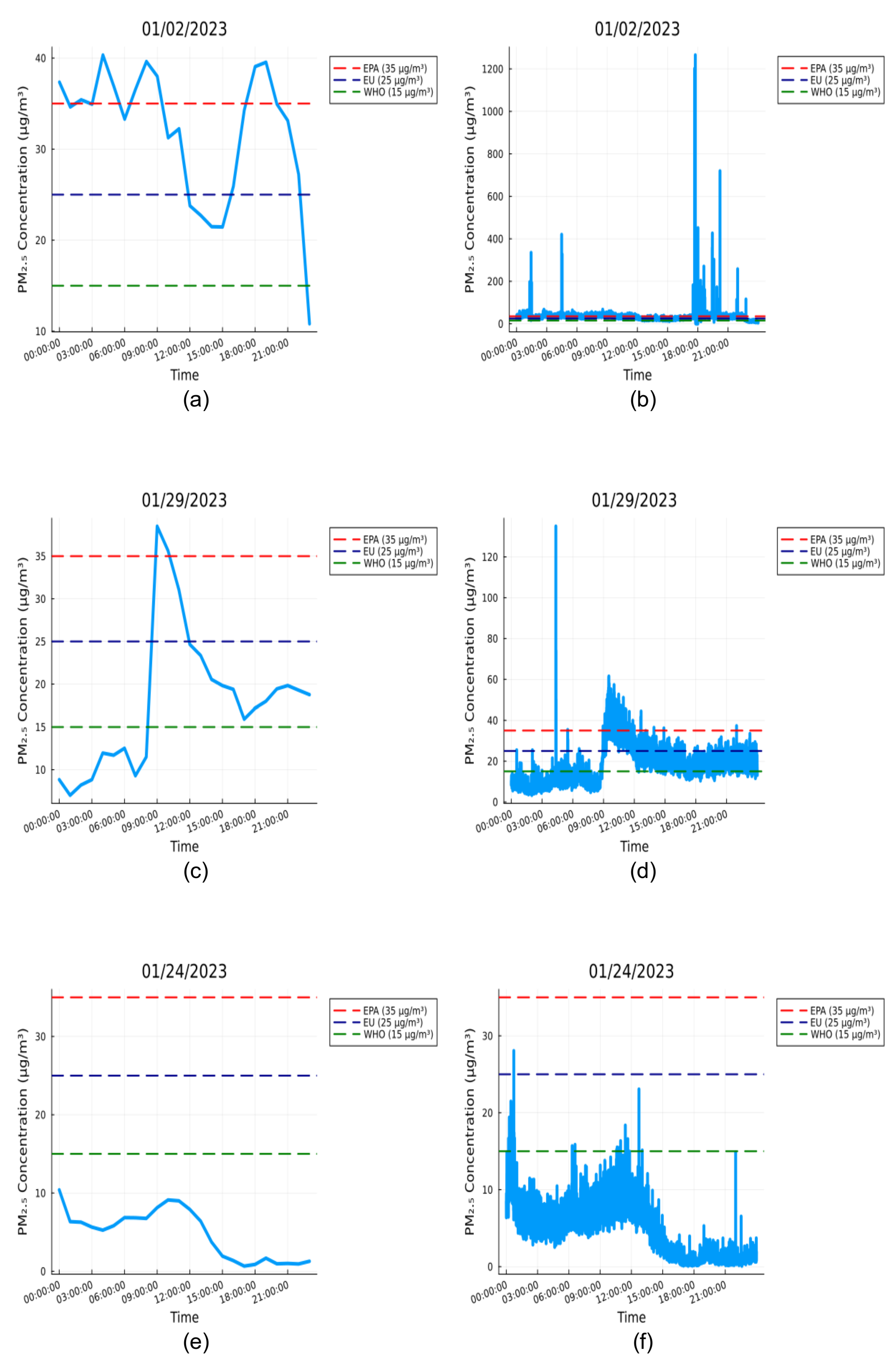
Figure 6.
Variogram plots of Concentration in decreasing order of pollution ( January 2nd January 29th, and January 24th). Figures (a), (c), and (e) represent Window Number 10 for the above mentioned days, while figures (b), (d), and (f) represent Window Number 50,000 for the same days.
Figure 6.
Variogram plots of Concentration in decreasing order of pollution ( January 2nd January 29th, and January 24th). Figures (a), (c), and (e) represent Window Number 10 for the above mentioned days, while figures (b), (d), and (f) represent Window Number 50,000 for the same days.
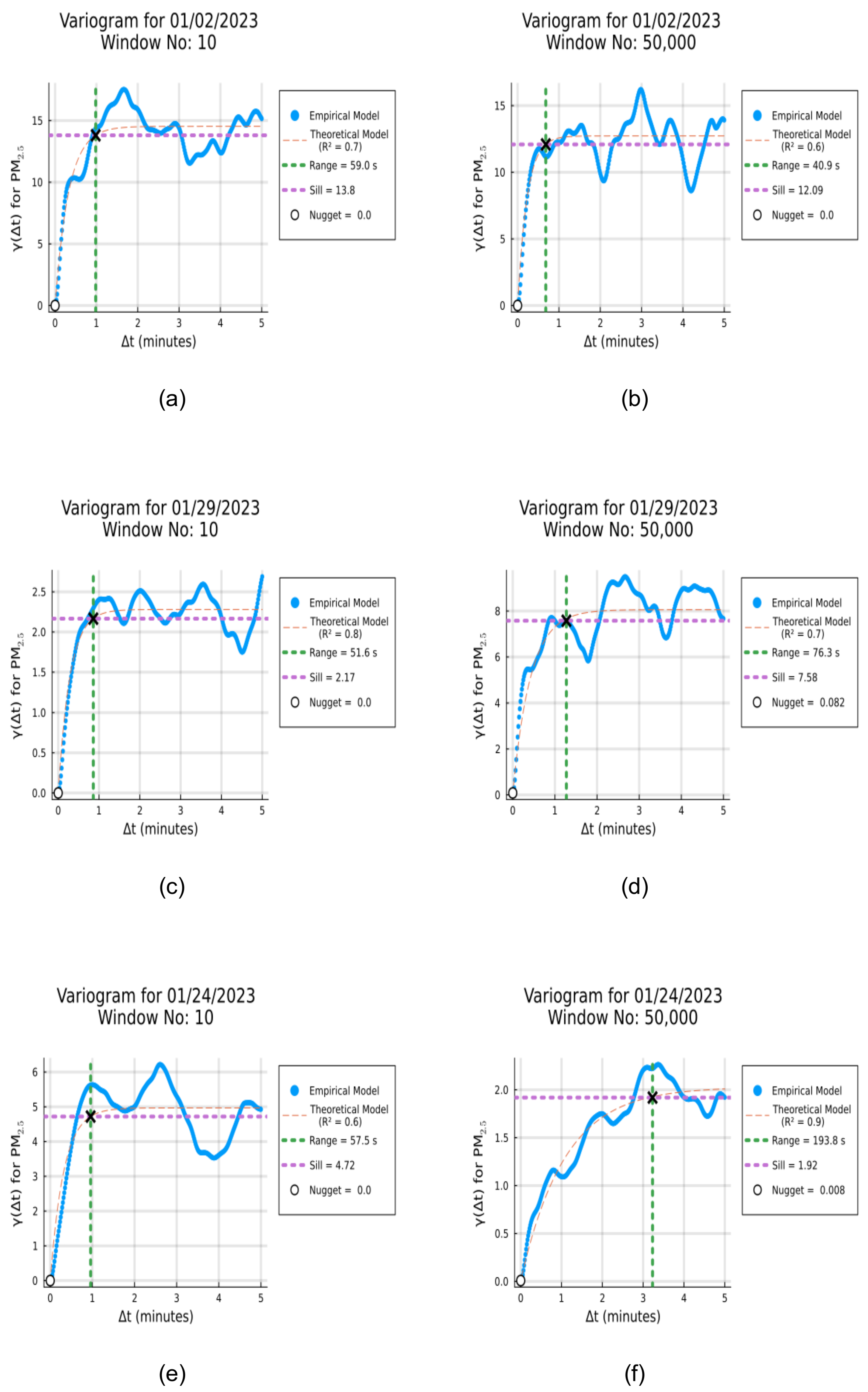
Figure 7.
Probability Density Plot of Measurement Time across 3 distinctly polluted days of January 2023.
Figure 7.
Probability Density Plot of Measurement Time across 3 distinctly polluted days of January 2023.
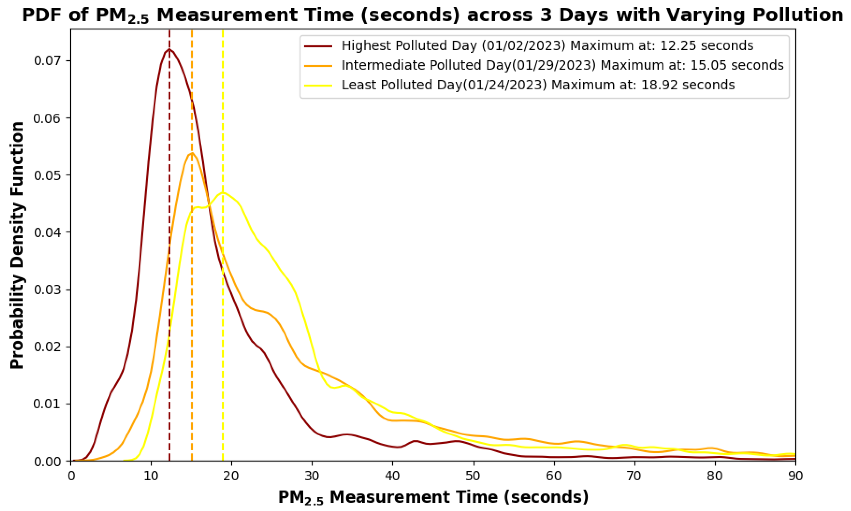
Figure 8.
Scatter plots of the Hyperparameter-Optimized Random Forest Regression Models of PM Measurement Time (minutes). The plot displays RFR models of various PM size fractions, with Panels a-g representing , ,, , , , and respectively
Figure 8.
Scatter plots of the Hyperparameter-Optimized Random Forest Regression Models of PM Measurement Time (minutes). The plot displays RFR models of various PM size fractions, with Panels a-g representing , ,, , , , and respectively
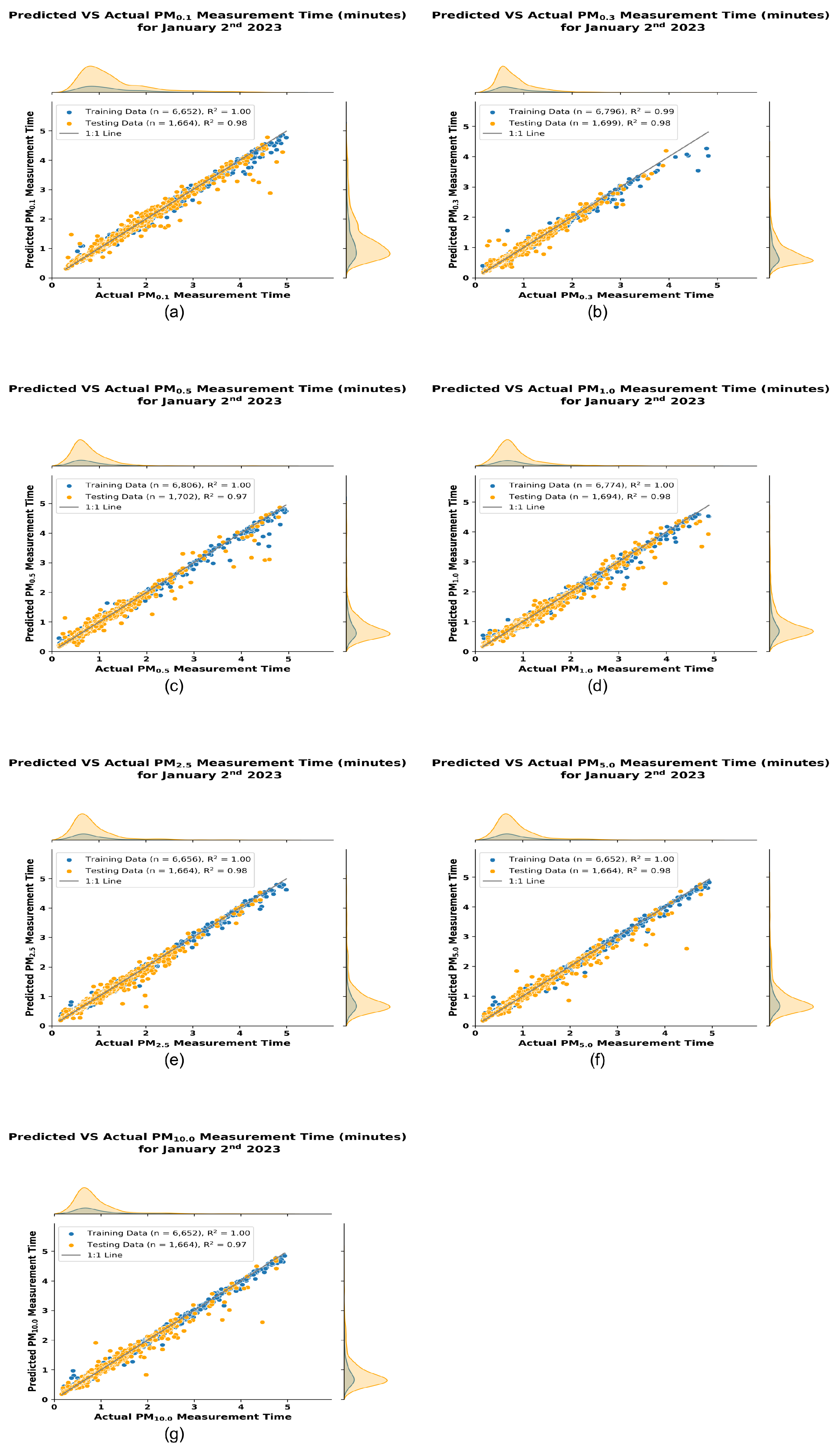
Figure 9.
Permutation Ranking of Features for the Hyperparameter Optimized Random Forest Regression Models of PM Measurement Time (minutes). The plot displays various PM size fractions, with Panels a-g representing , ,, , , , and respectively.
Figure 9.
Permutation Ranking of Features for the Hyperparameter Optimized Random Forest Regression Models of PM Measurement Time (minutes). The plot displays various PM size fractions, with Panels a-g representing , ,, , , , and respectively.
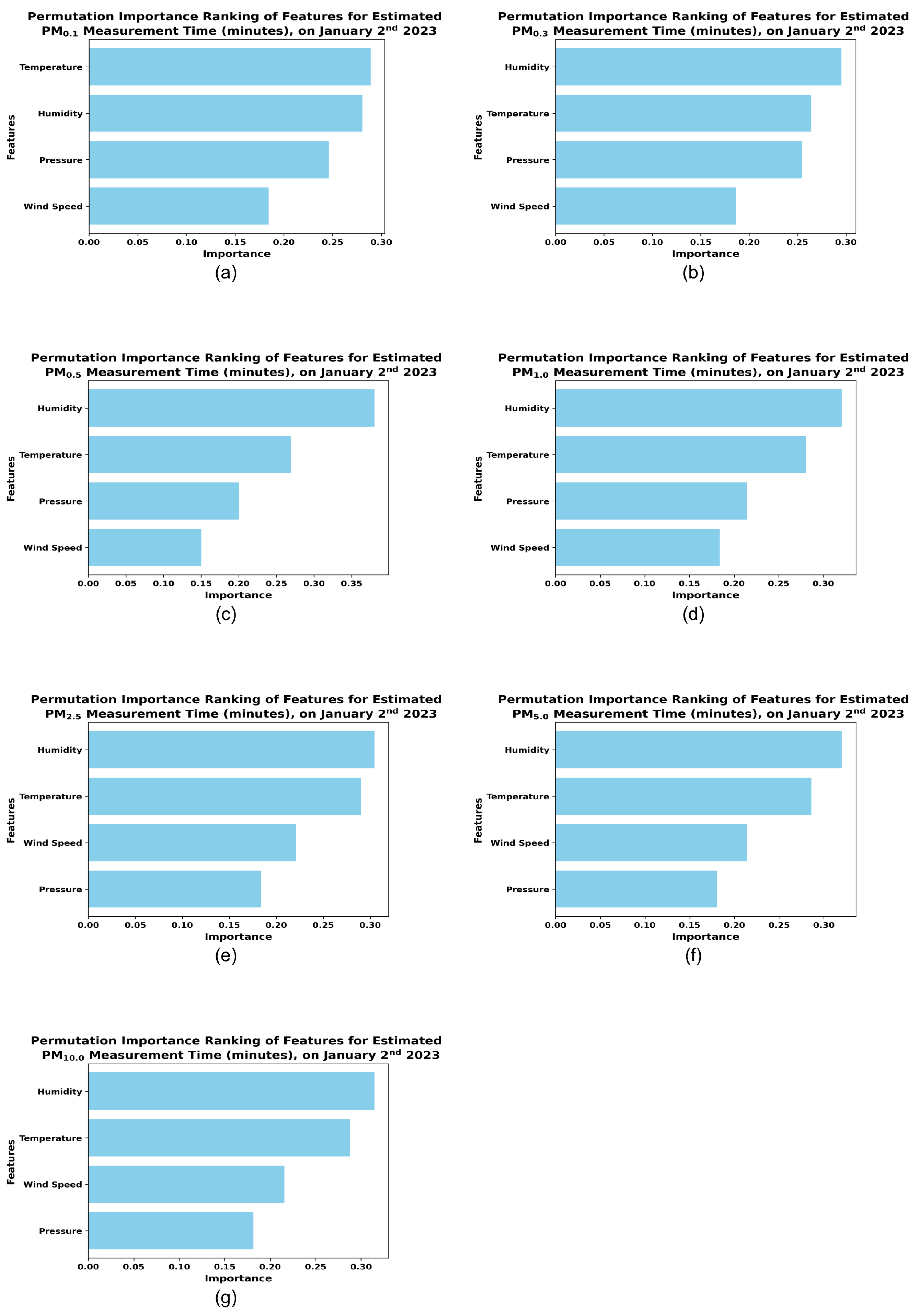
Table 1.
Sensor Specifications and Parameters Considered for the Study.
| Sensors | Parameters | Unit | Measurement Range | Resolution (seconds) |
|---|---|---|---|---|
| IPS7100 | ≤ 0.1 | 1 | ||
| ≤ 0.3 | 1 | |||
| ≤ 0.5 | 1 | |||
| ≤ 1.0 | 1 | |||
| ≤ 2.5 | 1 | |||
| ≤ 5.0 | 1 | |||
| ≤ 10.0 | 1 | |||
| BME280 | Temperature | °C | -40 – 85 | 10 |
| Atmosphric Pressure | hPa | 300 – 1100 | 10 | |
| Humidity | % | 0 – 100 | 10 | |
| AirMar | Wind Speed | m/s | 0 – 30 | 10 |
Table 3.
Statistical Summary of Concentration for the selected days.
| Dates | January 2nd | January 29th | January 24th |
|---|---|---|---|
| Count | 86400 | 86400 | 86400 |
| Mean | 31.87 | 17.97 | 4.80 |
| Std Dev | 21.91 | 8.93 | 3.35 |
| Min | 0.00 | 3.29 | 0.07 |
| 25% | 25.40 | 10.62 | 1.34 |
| 50% | 31.23 | 17.23 | 5.18 |
| 75% | 36.90 | 22.04 | 7.19 |
| Max | 1265.41 | 135.04 | 28.06 |
Table 4.
Estimated Sampling Time for 3 Distinctly Polluted Days in Increasing Order.
| Day | Peak Measurement Time (seconds) |
|---|---|
| Jan 2nd | 12.25 |
| Jan 29th | 15.05 |
| Jan 24th | 18.92 |
Table 5.
Coefficient Determination () and Mean Squared Error (MSE) for the Machine Learning Models.
| PM Measurement Time | Training | MSE Training | Testing | MSE Testing |
|---|---|---|---|---|
| 1.00 | 0.0015 | 0.98 | 0.0118 | |
| 1.00 | 0.0011 | 0.98 | 0.0051 | |
| 1.00 | 0.0012 | 0.97 | 0.0091 | |
| 1.00 | 0.0011 | 0.98 | 0.0102 | |
| 1.00 | 0.0009 | 0.98 | 0.0061 | |
| 1.00 | 0.0009 | 0.98 | 0.0085 | |
| 1.00 | 0.0009 | 0.97 | 0.0087 |
Disclaimer/Publisher’s Note: The statements, opinions and data contained in all publications are solely those of the individual author(s) and contributor(s) and not of MDPI and/or the editor(s). MDPI and/or the editor(s) disclaim responsibility for any injury to people or property resulting from any ideas, methods, instructions or products referred to in the content. |
© 2024 by the authors. Licensee MDPI, Basel, Switzerland. This article is an open access article distributed under the terms and conditions of the Creative Commons Attribution (CC BY) license (http://creativecommons.org/licenses/by/4.0/).
Copyright: This open access article is published under a Creative Commons CC BY 4.0 license, which permit the free download, distribution, and reuse, provided that the author and preprint are cited in any reuse.


