
Submitted:
24 April 2025
Posted:
27 April 2025
You are already at the latest version
Abstract
Air pollution, particularly PM10 particulate matter, poses significant health risks including respiratory and cardiovascular diseases as well as cancer. Accurate identification of PM10 reduction factors is therefore essential for developing effective sustainable development strategies. This study evaluated the performance of three machine learning algorithms - Decision Trees (CART), Random Forest, and Cubist Rule - in predicting PM10 concentrations and estimating long-term trends following meteorological normalisation. The research focused on Tarnów, Poland (2010-2022), with comprehensive consideration of meteorological variability. Results demonstrated superior accuracy for the Random Forest and Cubist models (R² ~0.88-0.89, RMSE ~14 μg/m³) compared to CART (RMSE 19.96 μg/m³). Air temperature and boundary layer height emerged as the most significant predictive variables across all algorithms. The Cubist algorithm proved particularly effective in detecting the impact of policy interventions, making it valuable for air quality trend analysis. While the study confirmed a statistically significant annual PM10 decrease (0.83-1.03 μg/m³), concentrations persistently exceeded both updated EU air quality standards (2024) and WHO guidelines (2021).
Keywords:
PM10 particulate matter
; meteorological normalisation
; machine learning
; air quality
; air pollution trends
1. Introduction
PM10 contamination in the air has a strong impact on human health. According to the International Agency for Research on Cancer (IARC), air pollution is considered a mixture of potentially carcinogenic substances. PM10 particles can penetrate deep into the lungs, contributing to respiratory and cardiovascular problems. This impact is comparable to other significant health risks, such as tobacco smoking or an unhealthy diet. Long-term exposure is associated with reduced lung function, worsened asthma symptoms, and respiratory infections, especially in children. Among adults, the risk of ischemic heart disease and stroke increases—both of which are major causes of premature death linked to air pollution. In Poland, the number of premature deaths caused by particulate pollution was approximately 44,000 in 2012 and 43,000 in 2019.
An effective assessment of air pollution concentration trends is possible through the application of meteorological normalisation. This method was developed by Stuart K. Grange and David C. Carslaw [1,2]. This method makes it possible to eliminate the influence of meteorological conditions from the time series of air pollution concentrations. Meteorological normalisation (also known as deweathering) involves generating multiple concentration forecasts for random meteorological scenarios using developed supervised learning models, with the resulting values being averaged. As a result, it becomes possible to estimate non-parametric trend values of air pollution concentrations corresponding to averaged meteorological conditions. Meteorological normalisation is a relatively new method that has been used by many researchers for various scientific purposes in different regions of the world [1,2,3,4,5,6,7,8,9,10,11,12,13,14,15,16,17].
The Random Forest (RF) algorithm is commonly used in meteorological normalisation due to its robustness to missing data, multicollinearity among explanatory variables, and the relative simplicity of hyperparameter tuning [2,3,8]. Besides RF, the Gradient Boosted Regression Model (GBM) algorithm has also often been used for meteorological normalisation. [4,6]. These two algorithms are most often compared to each other because both are characterised by high prediction accuracy and low bias [1,5,9,16]. Mallet (2021) [16] testował the above methods. The GBM was able to explain 46% of the predicted variable (PM10). In the case of the Random Forest model, the coefficient of determination (R²) was 0.59, indicating that this model explained 59% of the variance in the predicted variable. Comparing the RF and GBM models in terms of NOx predictions, the values of the coefficient of determination were 0.73 and 0.76, respectively [9]. Moreover, it was shown that the Random Forest algorithm is characterised by lower systematic errors. Lovric et al. (2022) [5] compared the Random Forest algorithm (RF) and the Gradient Boosting Method (LightGBM) for predicting concentrations of particulate matters. In this case, they obtained similar results from the above models. RF achieved an R2 value of 0.78 and LightGBM a value of 0.77. The study conducted in London showed that the Random Forest algorithm has varying accuracy depending on the predicted substance (SO2, NO2 and NOx). For NOx and NO₂ on Marylebone Road, R² values of 0.82 and 0.83 were achieved, respectively. However for SO₂, the R² results were significantly lower, ranging from 0.63 to 0.67 [1]. This means that the methods under consideration have varying accuracy depending on the location of the study and the predicted substance. This is also confirmed by the studies carried out for 3 Chinese mega cities, where for many substances (PM2.5, PM10, NO2, SO2, CO, O3) R2 values ranging from 0.7 to 0.86 were obtained using the Random Forest algorithm [8].
The aim of this study was to compare the effectiveness of three machine learning models (decision trees, random forests, and Cubist Rules) in forecasting and estimating trends in PM10 concentrations based on normalised data. This task was undertaken due to the lack of comprehensive comparative analyses of various supervised learning algorithms regarding their impact on nonparametric estimation of pollution trends. In the study, boosted methods (GBM, LightGBM) were intentionally omitted, as the literature [1,5,16] indicates that they demonstrate comparable or lower accuracy compared to the Random Forest. Only Gagliardi and Andenna (2021) [9] observed slightly higher R2 (0.76 vs 0.73) for GBM; however, other metrics did not confirm its superiority. It was decided to use the Cubist Rules algorithm [18,19], which—unlike other ensemble methods—has not yet been used in meteorological normalisation. Its advantage is the better interpretability of the results and the ability to generate transparent decision rules while maintaining high accuracy. It is an ensemble algorithm that combines a tree-based approach with rule generation. The conducted analyses enabled the identification of the most effective algorithms for modelling normalised PM10 concentrations, which in turn allows for reliable trend estimation and assessment of the effectiveness of remedial actions.
2. Materials and Methods
2.1. Research Area
The location of the research area, along with the air quality monitoring station and the meteorological station, is shown in Figure 1. The city of Tarnów is located in the eastern part of the Małopolska voivodeship in Poland. It is located on the Tarnów Plateau at the boundary between the Sandomierz Basin and the Carpathian Foothills. The city is inhabited by 103,130 people (data for the year 2023). The area of the city is 72.38 km2.
The analysed period covered the years 2010–2022. During this time, a significant improvement in air quality was observed in terms of PM10 concentrations. The current allowable average annual level of PM10 concentration is 40 μg/m3. This limit was exceeded in the first three analysed years. The year 2013 was omitted due to data completeness being less than 50%. A decrease in PM10 concentrations was observed from 41.9 μg/m3 (2010) to 23.7 μg/m3 (2022) (Figure 2). Despite the 43.4% reduction through the years, average annual PM10 concentrations are still higher than the values set out in the recommendations issued by the WHO in 2021 (15 μg/m3) and the new guidelines adopted by the Council of the European Union in November 2024 (20 μg/m3). It was also found that the daily average standard was not met during the years 2010–2021 (Figure 3). Currently, it is permissible for air quality standards to be exceeded on 35 days per year, but the revised EU regulations [18] reduce this number to 18. Over these 12 years, two of them (2010 and 2012) exceeded the annual limit and only four (2015, 2019, 2020 and 2020) had fewer than thirty-five days per year on which the daily limit was exceeded.
2.2. Data Sources and Computational Methods
The data of hourly PM10 concentration for the period 2010 – 2022 were obtained from the database of the Chief Inspectorate of Environmental Protection [19], while meteorological data such as wind speed (ws), wind direction (wd), relative humidity (rh), air temperature (tt) and atmospheric pressure (pres) were obtained from the archives of the Institute of Meteorology and Water Management [20]. Boundary layer height (blh), Cloud base height (cbh) and surface net solar radiation (ssr) was obtained from reanalysis for the global climate and weather ERA5 [21].
The study compared three supervised learning algorithms classified as ensemble methods: Decision Tree (cart) [22], Random Forest (ranger) [23,24], and Cubist Rules (cubist) [25]. Based on the date, auxiliary variables were created, such as Julian day (jday), day of the week (wday), and hour of the day (hour), representing typical periods of changes in air pollution emissions due to anthropogenic activities. The date variable was converted into a numerical format of the date to reflect the trend. The dataset was divided into a training (80% of samples used to adjust the model parameters) set, and test (20% of samples used to evaluate the model performance) set. From the training set, a validation set was created for the purpose of applying the resampling method (10-fold cross-validation). The use of this method provides a reasonable estimation of model accuracy assessment parameters at a level similar to the test set during the hyperparameter tuning stage of individual algorithms. For hyperparameter optimisation, a racing method was applied based on the statistical significance of the configurations of individual algorithms from the ANOVA model [26]. The application of this method allowed for a reduction in computation time by approximately 20%. The best-performing algorithms were evaluated on the test set. The evaluation of the model was carried out using basic statistical metrics, i.e., FAC2 (fraction of predictions within a factor of two), MB (mean bias), MGE (mean gross error), NMB (normalised mean bias), NMGE (normalised mean gross error), RMSE (root mean squared error), r (Pearson correlation coefficient), COE (Coefficient of Efficiency), and IOA (Index of Agreement based on Willmott) [27].
In order to determine the importance of predicted variables, EMA (Exploratory Model Analysis) was conducted. The identification aimed to determine which meteorological data has the greatest impact on PM10 concentration. This method demonstrated how the model's performance would change when one of the variables was removed. The significance was presented as RMSE values. The higher the metric, the greater the importance of the explanatory variable. The use of RMSE as a consistent metric enabled uniform comparisons of the applied supervised learning algorithms [28].
The developed models were used to carry out meteorological normalisation of particulate matter (PM10). For this purpose, we used bootstrap [29] with the number of repetitions equal to 200 for each data record. Based on normalised data determined using three models (cart, ranger, cubist), the PM10 trend was identified using the Theil-Sen robust linear regression estimator [30].
3. Result and Discussion
3.1. Evaluating the Accuracy of Machine Learning Algorithms
Figure 4 shows a comparison of observations with modelling results based on the applied algorithm. Three reference lines were added to the plot. One of them represents perfect mapping, while the other two indicate the error margin corresponding to a twofold overestimation or underestimation. All models accurately predict PM10 concentrations below 100 µg/m3, as evidenced by the high density of observations along the ideal model line. Nonetheless, regardless of the applied algorithm, there are instances of twofold overestimations and underestimations of PM10 concentrations. According to FAC2 values (shown in Table 1), the frequency did not exceed 10% when using the Random Forest (ranger) and Cubist Rules (cubist). In the case of the decision tree algorithm (cart), the frequency was almost twice as high. It is worth noting that the obtained FAC2 values for the Random Forest and Cubist Rules are comparable to those reported in other studies. Lv et al. (2022) [8], using the Random Forest model for PM10, achieved a FAC2 value of 0.91.
Table 1 summarises the statistical metrics used to assess the accuracy of models based on the machine learning algorithm. For the Ranger and Cubist algorithms, similar accuracy metric values were obtained. The values of the normalised mean gross error (NMGE), the coefficient of efficiency (COE), and the Index of Agreement (IOA) are the same. Ranger reached the highest value of correlation coefficient (r): 0.89, Cubist had a slightly lower score: 0.88. The models differed by RMSE by 0.03 μg/m³. The models had opposite values of mean bias (MB). For Ranger, the parameter assumed a positive value, which indicates a tendency to overestimate the results. The negative result obtained for CART and Cubist indicates a tendency to underestimate the results. For all three models, the normalised mean bias (NMB) value hovered around zero, indicating that no model had a significant tendency to overestimate or underestimate. The statistics for the CART algorithm significantly deviate from those of the other two models. RMSE reached its highest value of 19.96 μg/m³. NMGE indicated that the uncertainty of the Ranger algorithm's forecasts occurs at a level of 39% of the mean value.
Compared to other studies, the machine learning models applied in this analysis exhibit varied effectiveness. Lv et al. (2022) [8] achieved a higher mean systematic error (MB ~0.11) with lower NMB and NMGE values, while the Random Forest model developed by Lovrića et al. (2022) [5] demonstrated a lower RMSE (10.47) compared to Mallet’s (2021) [16] result of 19.5. The best accuracy in terms of RMSE (5.39 µg/m³) was demonstrated by Gagliardi and Andenna (2021) [9], which maintained the same IOA value (0.76) and slightly lower R² (0.73). However, it pertained to nitrogen oxides (NOx) concentrations. In terms of the coefficient of determination R², the presented Random Forest (RF) model outperforms Mallet (2021) [16] (0.49-0.59), Grange and Carslaw (2019) [1] (0.54-0.71), and Gagliardi and Andenna (2021) [9], approaching to results achieved by Lv et al. (0.81-0.94) and Wu et al. (2022) [17] (0.52-0.94). These findings confirm that the effectiveness of models depends both on the applied algorithm and the specificity of the analysed environmental data. Additionally, the appropriate selection of parameters and consideration of the local context are crucial for accurate air quality modelling.
3.2. Importance Variable
The plot of the evaluation of the importance of an explanatory variable is shown in Figure 5. Boxplots demonstrate the change of RMSE value after deleting individual variables [31,32]. The line inside the box indicates the median for the series of permutations, while the grey dots represent outlier values. The dashed vertical lines denote the loss function values for each model. The value of the loss function is constant and depends on model structure. It reflects error in the absence of predictive variables. For CART, the value is 16.69 μg/m³, for Ranger 10.03 μg/m³, and for Cubist 9.29 μg/m³. The value of the loss function were similar for Ranger and Cubist. In all the applied algorithms, air temperature (tt) turned out to be the variable with the greatest impact on PM10 concentrations. The median error after removing this variable was 23.9 μg/m³ (ranger), 21.5 μg/m³ (cubist) and 31.6 μg/m³ (cart). The significant impact of temperature likely stems from its association with the seasonal variability of emissions in the municipal and residential sector [33] and the deterioration of the conditions of dispersion of pollutants in winter, associated with the frequent occurrence of stable atmospheric layers [34]. It is worth noting that the decision tree algorithm (cart) showed a particularly strong dependence on the variable temperature compared to other models. This is a consequence of the collinearity of explanatory variables. In this case, the tuning process focused on one variable (tt), which is highly correlated with the dependent variable (PM10).
Other variables affecting the result were boundary layer height (blh), date (date), and the day of the year from Julian calendar (jday). In the case of the Ranger algorithm, removing the blh variable increased the median RMSE to 21.7 μg/m³, while for Cubist the median increased to 19.1 μg/m³, and for CART to 26.1 μg/m³. Boundary layer height is associated with surface temperature inversion. This phenomenon at low elevation negatively affects the dispersion of pollutants. During weak air mass movements, PM10 concentrations accumulate at ground level [35,36]. The variable numerically defining the date is significant because it reflects changes in pollutant emissions. After removing the "date" variable, RMSE increased to 16.9 μg/m³ in Ranger, in Cubist to 18.0 μg/m³, and in CART to 22.0 μg/m³. For decision trees, the least significant variable turned out to be the one representing the day of the week (wday). Its removal resulted in an RMSE increase of only 0.2 μg/m³ compared to the value of the loss function for this model. The second variable that slightly impacts the prediction quality is cloud base height (cbh). The increase in RMSE for this parameter was only 0.6 μgm−3 compared to the value of the loss function. Calculations performed on the cubist model indicated a low impact of the direction of wind (wd_cut) and the variable representing the hour of measurement during the day (hour). For both variables, RMSE increased by just 1 μg/m³ compared to the value of the loss function.
In each model, the temperature (tt) and the boundary layer height (blh) were the most important. The results obtained are not always consistent with earlier studies on other types of pollution and localisation. For example, studies conducted in the Alps focusing on nitrogen dioxide (NO₂) revealed that the most important explanatory variable was temperature, while the second most significant variable was the Julian day (jday) [10]. The high importance of jday resulted from the fact that studies conducted in the Alps did not consider the blh variable, focusing solely on the temperature gradient.
On the other hand, studies conducted in Australia on PM10 revealed that the intensity of fires, trend, and temperature were more significant compared to wind speed and the boundary layer height. Other studies conducted in England on SO₂, NO₂ and NOx provided evidence of the high significance of wind speed (ws) compared to temperature [1]. This stands in opposition to the obtained research findings, though it relates specifically to gaseous air pollutants. However, as in the present study, variables such as Julian day (jday), hour (hour) or wind direction (wd_cut) were of little importance. Research conducted in southern Italy on NOx showed that the most significant variable was wind direction (wd_cut). This contrasts sharply with the findings of the presented studies, where this was typically a variable of little importance. It is essential to emphasise that the interpretation of the significance of explanatory variables depends on the type of substance and the location. The high importance of wind direction may be due to the location of the station, which is strongly influenced by emission sources located in a specific direction from the station. Caution should be exercised if results differ significantly from other studies. It is also important to consider the selection of an appropriate number of explanatory variables, as each of the aforementioned studies used non-standard quantities of explanatory variables.
3.3. Comparison of Particulate Matter Trends
The results of PM10 concentration trends are presented in Figure 6. The solid red line shows the trend estimate and the dashed red lines show the 95% confidence intervals for the trend based on resampling methods. For CART, the trend is -0.83 (0.89 – 0.78) μg/m³, for Cubist -1.03 (1.11 – 0.94) μg/m³, and for Ranger -0.97 (1.04 – 0.9) μg/m³. The trend line for each model has a negative slope coefficient despite discrepancies in the accuracy assessment results (see Section 3.1). It should be noted that the 95% confidence intervals of the trend obtained from the Cubist and Ranger algorithms overlap. This indicates that they are not statistically significantly different at the 95% confidence level. Therefore, we can conclude that regardless of the applied algorithm (ranger or cubist), the differing importance of individual variables yields a similar trend value. Moving forward, when obtaining similar accuracy assessment results, a statistically comparable trend value is achieved. However, referring to the trend result obtained for the CART model, it was found to be statistically significantly different from the other algorithms. Furthermore, the mean value of the obtained trend was lower by approximately 0.14 – 0.20 μg/m³. This indicates that choosing the decision tree model, which is characterised by distinctly lower evaluation parameters, tends to underestimate the PM10 trend level.
The variability of monthly average normalised concentrations, presented in Figure. 6, indicates that in the case of the CART model, it is not possible to detect interventions, thus limiting the application of the normalisation algorithm [1]. On the other hand, two distinct interventions were identified in the case of the other algorithms, where the cubist model proved to be more sensitive. This suggests that it may be significantly more useful for identifying the effects of remedial actions introduced. Mallet (2021) [16] also conducted an analysis of PM10 concentration trends using the Random Forest and Gradient Boosted Regression models. The results obtained from both models were very close (the difference was only 0.1 μg/m³) and accurately reflected actual data. Similarly to our research, they did not show statistically significant differences as their confidence intervals overlapped. This indicates that models with similar accuracy, but not necessarily consistent structures (e.g., in terms of variable importance), can yield statistically similar results in trend analysis.
4. Conclusions
The comparison of three algorithms reveals that the Random Forest (ranger) and Cubist Rules models achieved very similar accuracy in predicting PM10 concentrations. Ranger demonstrated a slightly higher Pearson correlation coefficient (0.89 vs 0.88 for Cubist), while cubist had a marginally lower RMSE (14.06 vs 14.09 μg/m³). Both models had identical values for the coefficient of efficiency (0.52) and Willmott's index of agreement (0.76). The CART model exhibited noticeably worse results across all metrics (RMSE: 19.96 μg/m³, COE: 0.33).
The variable importance analysis demonstrated that air temperature (tt) and boundary layer height (blh) were the most significant predictors across all models. Removing the temperature variable led to an increase in RMSE to over 20 μg/m³ (median: 23.9 for Ranger, 21.5 for Cubist, and 31.6 for CART), while removing blh resulted in an RMSE exceeding 19 μg/m³. Temporal variables, such as date and day of the year, also had a significant impact, whereas parameters like the day of the week or cloud base height proved to be of little importance.
Meteorological normalisation results demonstrated statistically significant downward PM10 trends across all models. The cubist model indicated the largest average annual decrease (-1.03 μg/m³), while the CART model showed the smallest (-0.83 μg/m³). It is important to note that the confidence intervals for cubist and ranger overlapped, signifying no significant difference between these models. The Cubist model proved particularly effective in identifying the impact of political interventions on air quality.
Despite the observed improvement in air quality (a 43.4% reduction in PM10 concentrations between 2010 and 2022), the annual average concentrations in Tarnów still exceed both WHO guidelines (15 μg/m³) and the new EU standards (20 μg/m³). These results emphasise the need for further remedial actions in air protection. This demonstrates that municipal interventions, such as emission reduction programs aimed at achieving the required air quality standards, are yielding benefits. While air quality in Tarnów is improving, continued mobilisation by the local government and residents is essential to strive for the achievement of the new, lower permissible PM10 concentration levels and other air pollution standards established by the European Parliament and the Council of the European Union.
Author Contributions
Conceptualization, M.R.; methodology, M.R.; software, K.G.; validation, K.G.; formal analysis, M.R. and K.G.; investigation, M.R. and K.G.; resources, M.R. and K.G.; data curation, K.G.; writing—original draft preparation, M.R. and K.G.; writing—review and editing, M.R. and K.G.; visualisation, K.G.; supervision, M.R.; project administration, M.R.; funding acquisition, M.R. K.G. 50% and M.R. 50 %
Funding
The work was carried out as part of research associated with the Ministry of Science and Higher Education (Poland) subsidy for AGH University of Krakow to maintain scientific potential (Contract no. 16.16.150.545) and “Excellence initiative – research university” program for AGH University of Krakow.
Institutional Review Board Statement
Not applicable.
Informed Consent Statement
Not applicable.
Data Availability Statement
The datasets of this study are not publicly available. However, they may be made available upon reasonable request by the author.
Conflicts of Interest
The authors declare no conflicts of interest.
Abbreviations
The following abbreviations are used in this manuscript:
| EU | European Union |
| WHO | World Health Organization |
| PM10 | Particulate matter |
| NOx | Nitrogen oxide |
| NO2 | Nitrogen dioxide |
| SO2 | Sulfur dioxide |
| CO | Carbon monoxide |
| O3 | Ozone |
| RF | Random Forest |
| GBM | Gradient Boosted Regression Model |
| ws | Wind speed |
| wd_cut | Wind direction |
| rh | Relative humidity |
| tt | Air temperature |
| pres | Atmospheric pressure |
| blh | Boundary layer height |
| cbh | Cloud base height |
| ssr | Surface net solar radiation |
| cart | Decision Tree Model |
| ranger | Random Forest Model |
| cubist | Cubist Rules Model |
| jday | Julian day |
| wday | Day of the week |
| hour | Hour of the day |
| FAC2 | Fraction of predictions within a factor of two |
| MB | The mean bias |
| MGE | The mean gross error |
| NMB | The normalised mean bias |
| NMGE | The normalised mean gross error |
| RMSE | The root mean square error |
| r | The Pearson correlation coefficient |
| COE | The Coefficient of Efficiency |
| IOA | The Index of Agreement based on Willmott |
| R2 | The coefficient of determination |
| EMA | Exploratory Model Analysis |
References
- Grange, S.K.; Carslaw, D.C. Using Meteorological Normalisation to Detect Interventions in Air Quality Time Series. Science of the Total Environment 2019, 653, 578–588. [CrossRef]
- Grange, S.K.; Carslaw, D.C.; Lewis, A.C.; Boleti, E.; Hueglin, C. Random Forest Meteorological Normalisation Models for Swiss PM10 Trend Analysis. 2018, 6223–6239.
- V. Vu, T.; Shi, Z.; Cheng, J.; Zhang, Q.; He, K.; Wang, S.; M. Harrison, R. Assessing the Impact of Clean Air Action on Air Quality Trends in Beijing Using a Machine Learning Technique. Atmos Chem Phys 2019, 19, 11303–11314. [CrossRef]
- Ceballos-Santos, S.; González-Pardo, J.; Carslaw, D.C.; Santurtún, A.; Santibáñez, M.; Fernández-Olmo, I. Meteorological Normalisation Using Boosted Regression Trees to Estimate the Impact of COVID-19 Restrictions on Air Quality Levels. International Journal of Environmental Research and Public Health 2021, Vol. 18, Page 13347 2021, 18, 13347. [CrossRef]
- Lovrić, M.; Antunović, M.; Šunić, I.; Vuković, M.; Kecorius, S.; Kröll, M.; Bešlić, I.; Godec, R.; Pehnec, G.; Geiger, B.C.; et al. Machine Learning and Meteorological Normalization for Assessment of Particulate Matter Changes during the COVID-19 Lockdown in Zagreb, Croatia. International Journal of Environmental Research and Public Health 2022, Vol. 19, Page 6937 2022, 19, 6937. [CrossRef]
- Munir, S.; Coskuner, G.; Jassim, M.S.; Aina, Y.A.; Ali, A.; Mayfield, M. Changes in Air Quality Associated with Mobility Trends and Meteorological Conditions during COVID-19 Lockdown in Northern England, UK. Atmosphere 2021, Vol. 12, Page 504 2021, 12, 504. [CrossRef]
- Petetin, H.; Bowdalo, D.; Soret, A.; Guevara, M.; Jorba, O.; Serradell, K.; Pérez García-Pando, C. Meteorology-Normalized Impact of the COVID-19 Lockdown upon NO2 Pollution in Spain. Atmos Chem Phys 2020, 20, 11119–11141. [CrossRef]
- Lv, Y.; Tian, H.; Luo, L.; Liu, S.; Bai, X.; Zhao, H.; Lin, S.; Zhao, S.; Guo, Z.; Xiao, Y.; et al. Meteorology-Normalized Variations of Air Quality during the COVID-19 Lockdown in Three Chinese Megacities. Atmos Pollut Res 2022, 13, 101452. [CrossRef]
- Gagliardi, R.V.; Andenna, C. Machine Learning Meteorological Normalization Models for Trend Analysis of Air Quality Time Series. International Journal of Environmental Impacts 2021, 4, 375–387. [CrossRef]
- Falocchi, M.; Zardi, D.; Giovannini, L. Meteorological Normalization of NO2 Concentrations in the Province of Bolzano (Italian Alps). Atmos Environ 2021, 246, 118048. [CrossRef]
- Zheng, H.; Kong, S.; Zhai, S.; Sun, X.; Cheng, Y.; Yao, L.; Song, C.; Zheng, Z.; Shi, Z.; Harrison, R.M. An Intercomparison of Weather Normalization of PM2.5 Concentration Using Traditional Statistical Methods, Machine Learning, and Chemistry Transport Models. npj Climate and Atmospheric Science 2023 6:1 2023, 6, 1–10. [CrossRef]
- Ali-Taleshi, M.S.; Riyahi Bakhtiari, A.; K. Hopke, P. Meteorologically Normalized Spatial and Temporal Variations Investigation Using a Machine Learning-Random Forest Model in Criteria Pollutants across Tehran, Iran. Urban Clim 2024, 53, 101790. [CrossRef]
- Kamińska, J.A. A Random Forest Partition Model for Predicting NO2 Concentrations from Traffic Flow and Meteorological Conditions. Science of The Total Environment 2019, 651, 475–483. [CrossRef]
- Kamińska, J.A. The Use of Random Forests in Modelling Short-Term Air Pollution Effects Based on Traffic and Meteorological Conditions: A Case Study in Wrocław. J Environ Manage 2018, 217, 164–174. [CrossRef]
- Cole, M.A.; Elliott, R.J.R.; Liu, B. The Impact of the Wuhan Covid-19 Lockdown on Air Pollution and Health: A Machine Learning and Augmented Synthetic Control Approach. Environ Resour Econ (Dordr) 2020, 76, 553–580. [CrossRef]
- Mallet, M.D. Meteorological Normalisation of PM10 Using Machine Learning Reveals Distinct Increases of Nearby Source Emissions in the Australian Mining Town of Moranbah. Atmos Pollut Res 2021, 12, 23–35. [CrossRef]
- Wu, Q.; Li, T.; Zhang, S.; Fu, J.; Seyler, B.C.; Zhou, Z.; Deng, X.; Wang, B.; Zhan, Y. Evaluation of NOx Emissions before, during, and after the COVID-19 Lockdowns in China: A Comparison of Meteorological Normalization Methods. Atmos Environ (1994) 2022, 278, 119083. [CrossRef]
- European Parliament; of the European Union, C. Directive (EU) 2024/2881 of the European Parliament and of the Council of 23 October 2024 on Ambient Air Quality and Cleaner Air for Europe. Official Journal of the European Union 2024, L series, 1–30.
- Chief Inspectorate of Environmental Protection (GIOS) Air Quality Monitoring Archive 2025.
- Institute of Meteorology; (IMGW-PIB), W.M. Public Data Portal 2025.
- Hersbach, H., Bell, B., Berrisford, P., Biavati, G., Horányi, A., Muñoz Sabater, J., Nicolas, J., Peubey, C., Radu, R., Rozum, I., Schepers, D., Simmons, A., Soci, C., Dee, D., Thépaut, J.-N. ERA5 Hourly Data on Single Levels from 1979 to Present (accessed on 27 September 2021).
- Rokach, L.; Maimon, O. Decision Trees. In Data Mining and Knowledge Discovery Handbook; Rokach, L., Maimon, O., Eds.; Springer: Boston, MA, 2005; pp. 165–192 ISBN 038725465X.
- Breiman, L. Random Forests. Mach Learn 2001, 45, 5–32. [CrossRef]
- Wright, M.N.; Ziegler, A. Ranger: A Fast Implementation of Random Forests for High Dimensional Data in C++ and R. J Stat Softw 2017, 77, 1–17. [CrossRef]
- Quinlan, J.R. Combining Instance-Based and Model-Based Learning. International Conference on Machine Learning 1993, 236–243. [CrossRef]
- Kuhn, M.; Wickham, H. Tidymodels: A Collection of Packages for Modeling and Machine Learning Using Tidyverse Principles Available online: https://www.tidymodels.org (accessed on 20 May 2024).
- Carslaw, D.C.; Ropkins, K. Openair - An r Package for Air Quality Data Analysis. Environmental Modelling and Software 2012, 27–28, 52–61. [CrossRef]
- Biecek, P.; Burzykowski, T. Explanatory Model Analysis; Chapman and Hall/CRC: New York, 2021; ISBN 9780367135591.
- Kunsch, H.R. Annals of Statistics. The jackknife and the bootstrap for general stationary observations 1989, 17, 1217–1241.
- Wang, X.; Yu, Q. Unbiasedness of the Theil–Sen Estimator. J Nonparametr Stat 2005, 17, 685–695. [CrossRef]
- Biecek, P.; Burzykowski, T. Explanatory Model Analysis; Chapman and Hall/CRC, New York, 2021;
- Biecek, P. DALEX: Explainers for Complex Predictive Models in R. Journal of Machine Learning Research 2018, 19, 1–5.
- Szulecka, A.; Oleniacz, R.; Rzeszutek, M. Functionality of Openair Package in Air Pollution Assessment and Modeling — a Case Study of Krakow. Environmental Protection and Natural Resources 2017, 28, 22–27. [CrossRef]
- Oleniacz, R.; Bogacki, M.; Szulecka, A.; Rzeszutek, M.; Mazur, M. Assessing the Impact of Wind Speed and Mixing-Layer Height on Air Quality in Krakow ( Poland ) in the Years 2014-2015. Journal of Civil Engineering, Environment and Architecture 2016, XXXIII, 315–342. [CrossRef]
- Foskinis, R.; Gini, M.I.; Kokkalis, P.; Diapouli, E.; Vratolis, S.; Granakis, K.; Zografou, O.; Komppula, M.; Vakkari, V.; Nenes, A.; et al. On the Relation between the Planetary Boundary Layer Height and in Situ Surface Observations of Atmospheric Aerosol Pollutants during Spring in an Urban Area. Atmos Res 2024, 308, 107543. [CrossRef]
- Du, C.; Liu, S.; Yu, X.; Li, X.; Chen, C.; Peng, Y.; Dong, Y.; Dong, Z.; Wang, F. Urban Boundary Layer Height Characteristics and Relationship with Particulate Matter Mass Concentrations in Xi’an, Central China. Aerosol Air Qual Res 2013, 13, 1598–1607. [CrossRef]
Figure 1.
Graphical representation of the location of measurement stations.
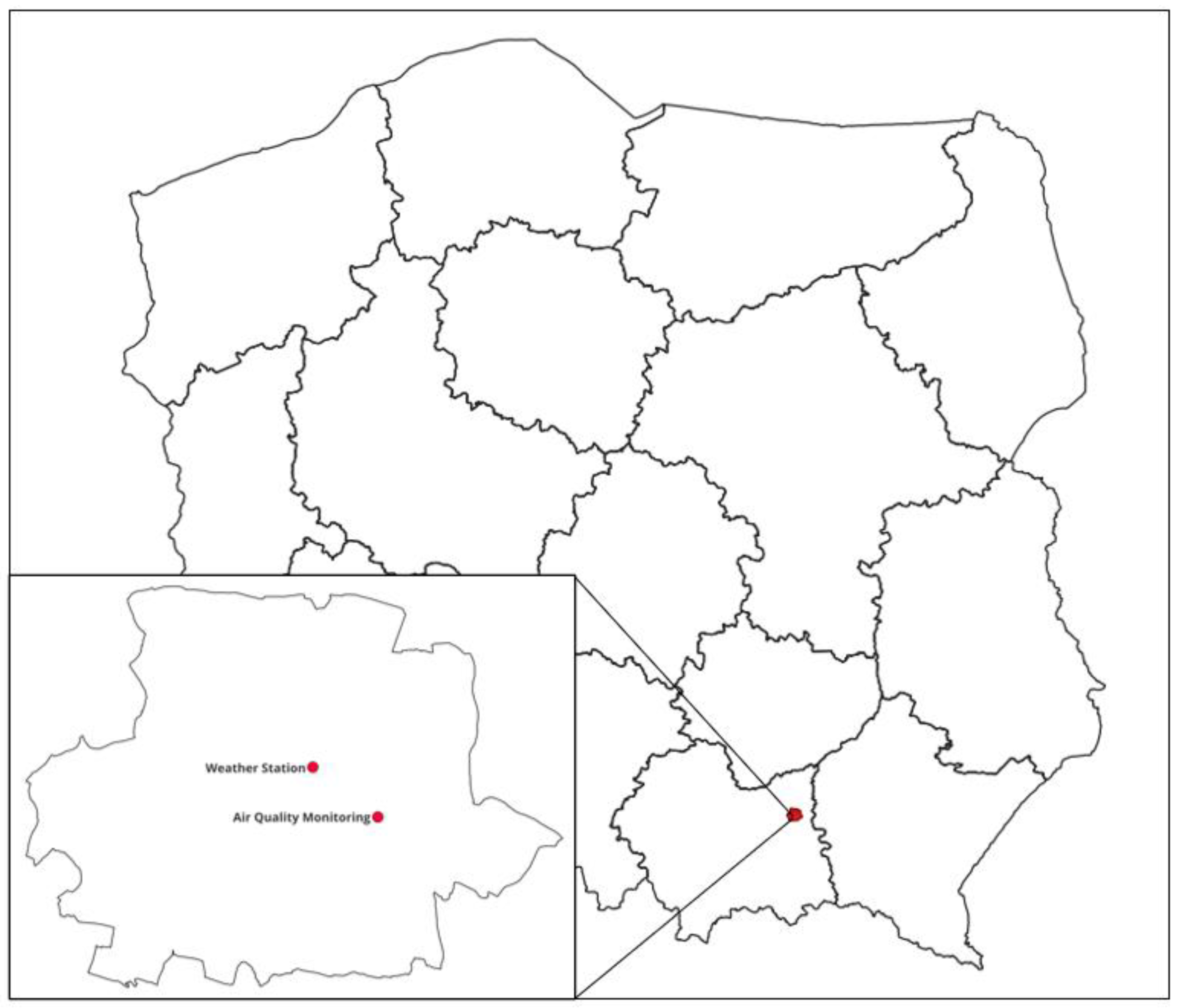
Figure 2.
Distribution of average annual PM10 concentrations.
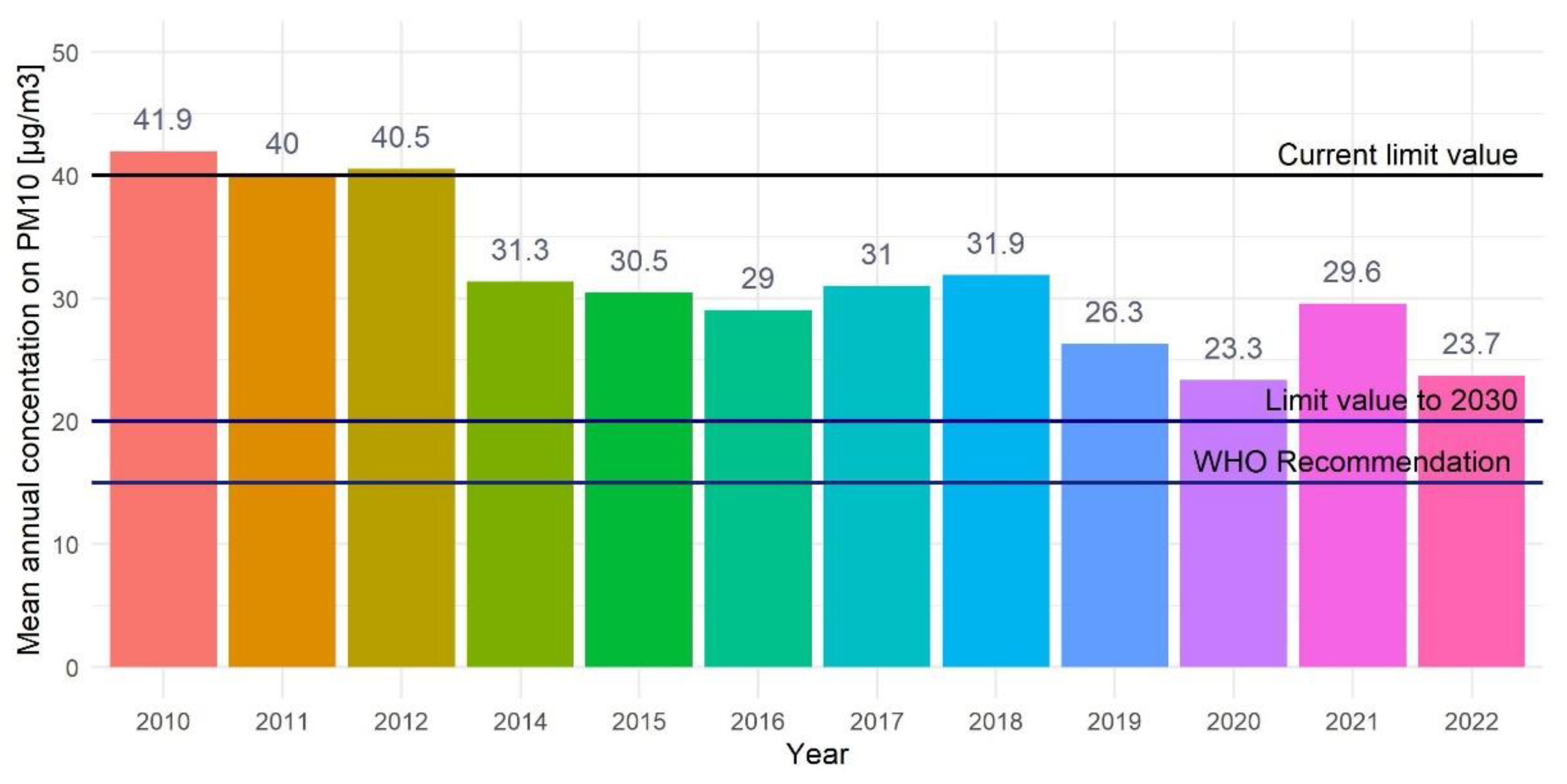
Figure 3.
Distribution of days in year when the daily average air quality standard for PM10 was exceeded.
Figure 3.
Distribution of days in year when the daily average air quality standard for PM10 was exceeded.
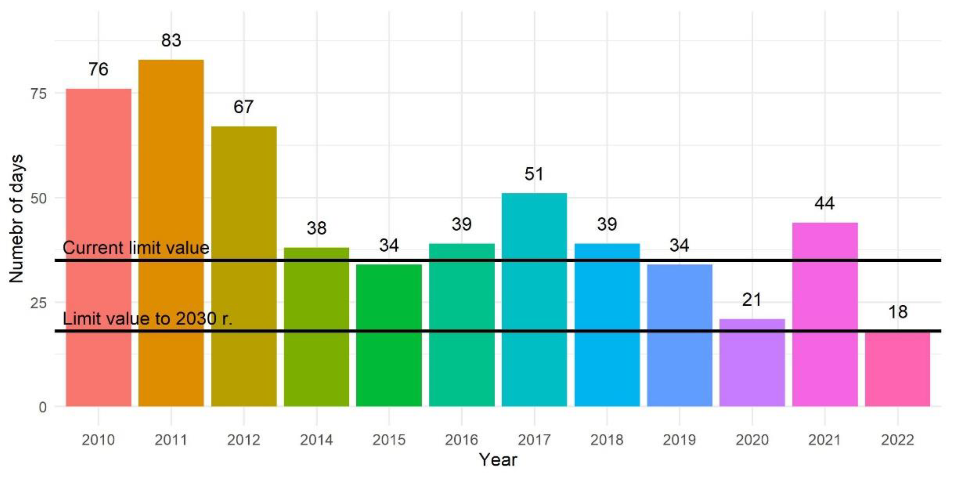
Figure 4.
Scatterplot of the comparison of PM10 observations with modelling results on the test dataset for three machine learning algorithms.
Figure 4.
Scatterplot of the comparison of PM10 observations with modelling results on the test dataset for three machine learning algorithms.
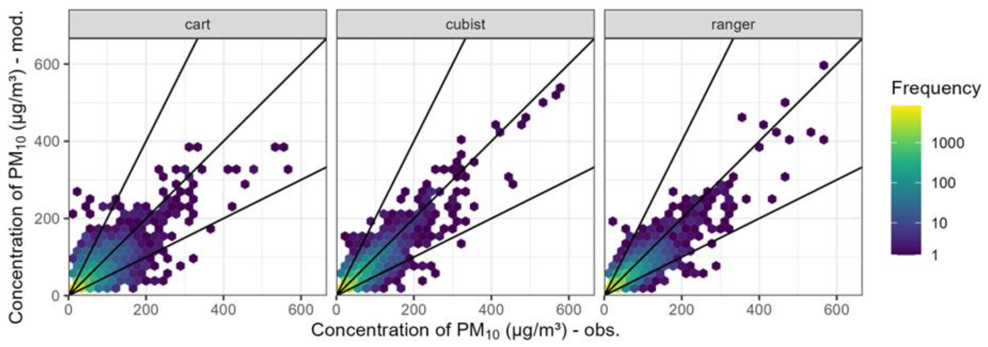
Figure 5.
Measure of importance of predictor variables for three machine learning algorithms.
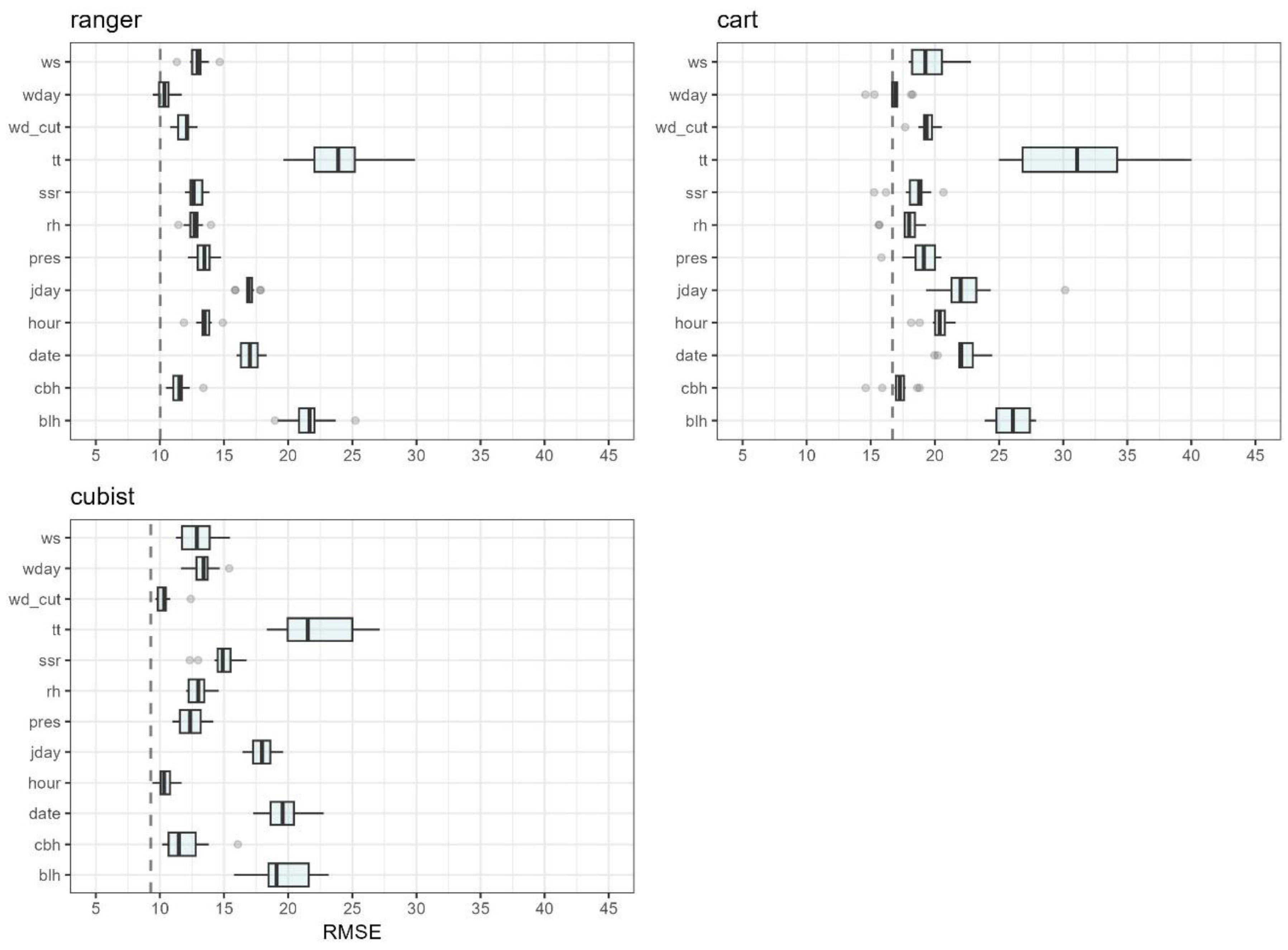
Figure 6.
Graphical representation of the PM10 concentration trend with 95% confidence intervals, determined using three machine learning algorithms.
Figure 6.
Graphical representation of the PM10 concentration trend with 95% confidence intervals, determined using three machine learning algorithms.
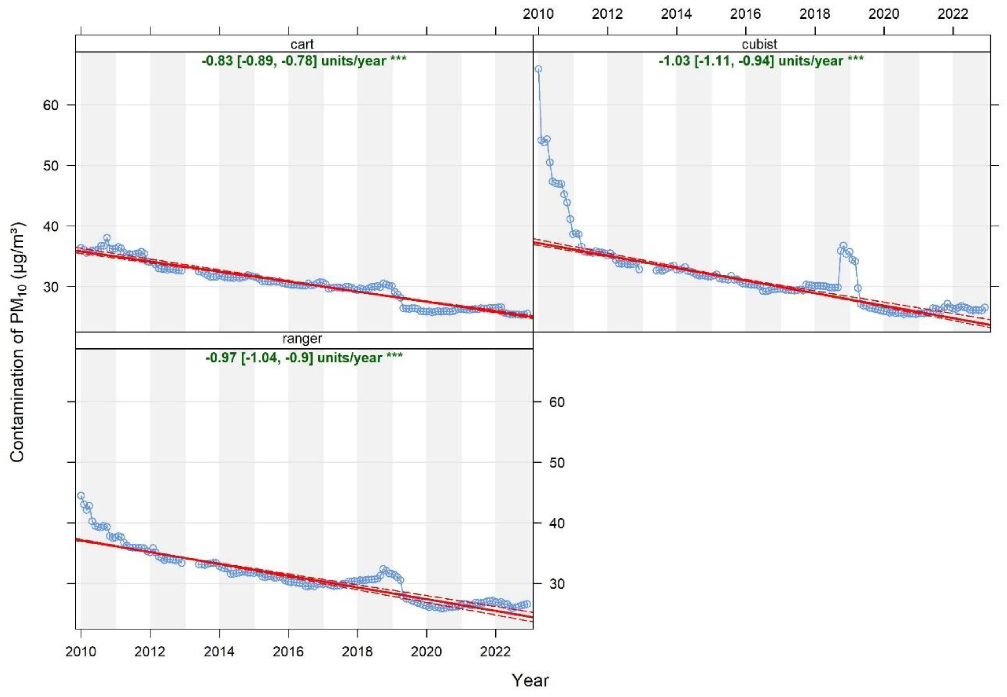

Table 1.
Summary of model accuracy metrics depending on the supervised learning algorithm used.
| Model | FAC2 | MB | MGE | NMB | NMGE | RMSE | r | COE | IOA |
| Cart | 0.82 | -0.14 | 11.94 | -0.001 | 0.39 | 19.96 | 0.75 | 0.33 | 0.66 |
| Cubist | 0.90 | -0.11 | 8.52 | -0.040 | 0.28 | 14.06 | 0.88 | 0.52 | 0.76 |
| Ranger | 0.91 | 0.11 | 8.46 | 0.004 | 0.28 | 14.09 | 0.89 | 0.52 | 0.76 |
Disclaimer/Publisher’s Note: The statements, opinions and data contained in all publications are solely those of the individual author(s) and contributor(s) and not of MDPI and/or the editor(s). MDPI and/or the editor(s) disclaim responsibility for any injury to people or property resulting from any ideas, methods, instructions or products referred to in the content. |
© 2025 by the authors. Licensee MDPI, Basel, Switzerland. This article is an open access article distributed under the terms and conditions of the Creative Commons Attribution (CC BY) license (http://creativecommons.org/licenses/by/4.0/).
Copyright: This open access article is published under a Creative Commons CC BY 4.0 license, which permit the free download, distribution, and reuse, provided that the author and preprint are cited in any reuse.


