Submitted:
18 October 2024
Posted:
21 October 2024
Read the latest preprint version here
Abstract
This paper discusses the problem of the fastest motion of an object in a curved earth tunnel. By establishing a mathematical model and applying the Python visualization toolkit, the analytical expression of the brachistocentre is derived, and the physical meaning of the integral constant C is analyzed . The study found that under certain conditions, a curved tunnel can provide a shorter travel time than a straight tunnel, which challenges intuitive cognition . At the same time, this research method that combines mathematical software and physical models can help students better expand their thinking about physical models, making complex expanded physical models easy to understand and master .
Keywords:
Earth tunnel
; fastest motion
; Python visualization toolkit
The Earth Tunnel Problem, as a widely discussed model, has been discussed in many studies [1,2,3,4,5,6,7,8], and many literary and film works have also proposed their own corresponding ideas. For example, Jules Verne's famous science fiction work "Journey to the Center of the Earth" imagines a hypothetical tunnel that passes through the center of the earth and runs through the two ends of the earth - people can go through this tunnel directly to the two ends of the earth and enjoy the fantastic beauty of the center of the earth along the way; "Total Recall" and "Earth Cannon" "realized" Verne's dream. However, the discussion so far is limited to the case where the shape of the tunnel is set to a straight line. So, if the Earth tunnel between any two points on the surface of the earth is not limited in shape, is the fastest travel time still 42 minutes? In this article , the author will take this as the starting point, and with the help of the Python visualization toolkit, clarify what kind of analytical curve must be followed to open a fastest Earth tunnel (regardless of shape) between any two points on the surface of the earth, and what related properties of this curve.
1. Model Establishment
To solve the problem of curved earth tunnels, we first establish a model : assume that the earth is a uniform sphere with a radius of R , a mass of M , and a density of ρ , then dig a (curved) tunnel of unlimited shape, regard any object in the tunnel as a mass point m , r is the distance between the mass point and the center of the earth , and establish a polar coordinate system with the center of the earth as the origin (as shown in Figure 1) . Ignore the centrifugal inertia of the earth's rotation , the Coriolis force , the size of the tunnel, the friction in the tunnel, etc. , and discuss the movement of the mass point under the condition of only considering the action of universal gravitation .
2. Python Visualization Toolkit Analysis Modeling
2.1. Theoretical Modeling Process
According to Gauss's theorem, take any point (r,θ ) inside the earth , then the gravity of the particle at that point points to the center of the sphere, and the magnitude is
Let , assuming that the infinite distance outside the earth is the potential energy zero point, then the gravitational potential energy of a point (r,θ) inside the earth is:
Then, the energy conservation equation for the process of moving from a point on the earth's surface to a point inside the earth (r0 ,θ0) is listed as follows:
It can be solved
At the same time, according to the representation of velocity in polar coordinate system
the time T required to travel from one point A on the Earth's surface to another point B on the Earth's surface.
To find out where the minimum value of T is obtained, let (where ) , that is, to solve the minimum point (extreme point) of f (r) . According to the Euler-Lagrange equation, if the function T is required to obtain an extreme value, the function f (r) needs to satisfy the equation
To solve the differential equation more simply, we can use it to transform it into
Convert to
Assuming that θ 0 is the direction angle of the particle at the initial moment, then solving the transformed differential equation, we can finally obtain the analytical expression of the fastest descent line inside the earth in the polar coordinate system:
① ( )
② ( , are the endpoint values of the fastest curve )
Due to the domain of the inverse sine function, the premise for the analytical expression ① to be meaningful is
That is
2.2. Python Visualization Code
2.2.1. Visual Code Design Ideas
(1)Functionthetar
This function is used to calculate a certain θ under a certain r and the angle value θ 0 of the direction where the particle is located at the initial moment according to the analytical formula of the fastest curve ① . The input parameters are r , R , C and θ0 are calculated and output in two cases :
①At that time ,
② Otherwise , still according to the calculation
(2) Function plot_q
This function is used to draw the fastest curve when C is a specific value . The thetar function needs to be called to calculate the coordinates of each point required to draw the graph.
(3) Main program
Set R (for the convenience of drawing, set R to 1) and the angle value θ 0 of the direction where the particle is located at the initial moment , and call the function plot_q to draw the fastest curve under different C values .
For each C value, the plot_q function is called to draw the corresponding curve and set the legend. Finally, plt.show() is used to display a series of images of the fastest curves under different C values .
2.2.2. Visualization Code and Visualization Results
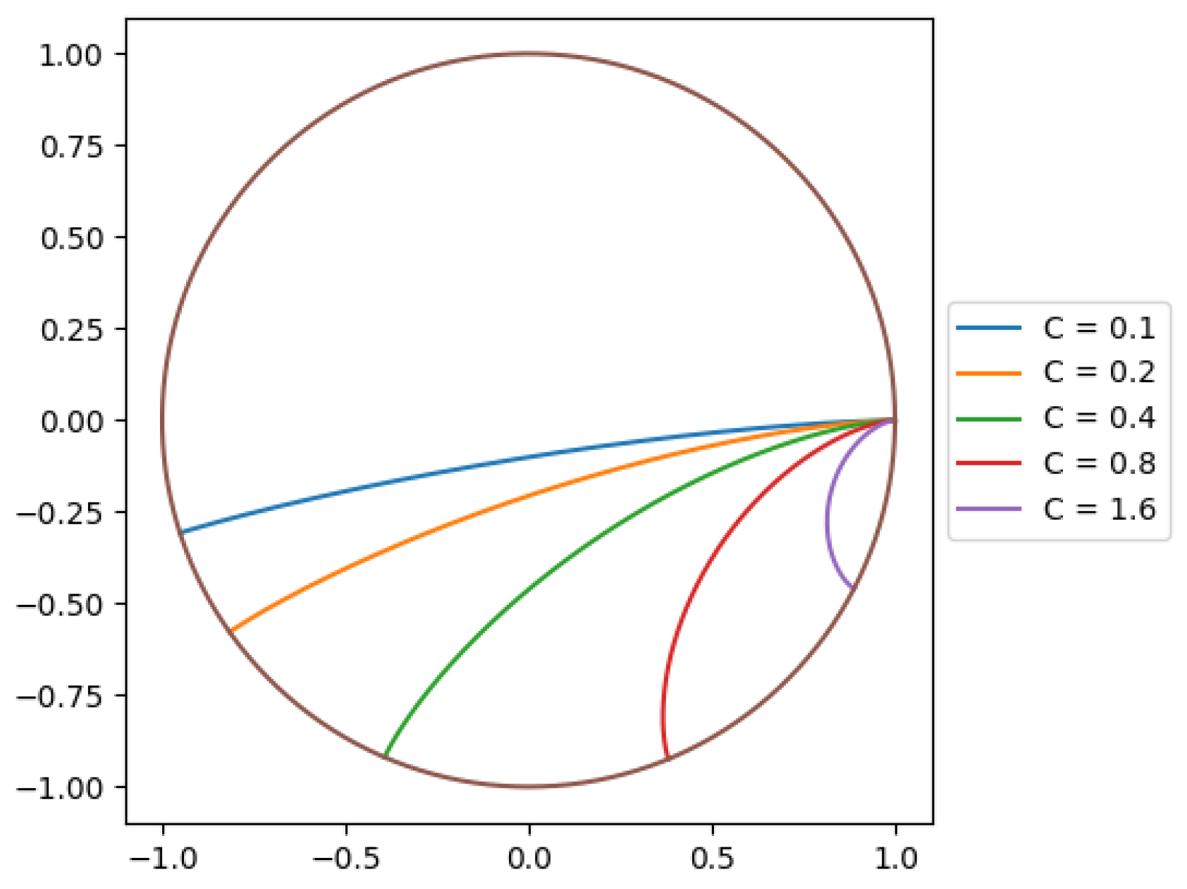
According to the design ideas described in Section 2.2.1 , the visualization code is shown above (which is also shown in Figure 2), and the visualization result is shown in Figure 3 .
import matplotlib.pyplot as plt
import math
def thetar(r,R,C,theta_0):
if abs(C*math.sqrt(R**2/r**2-1)-1)<1.0e-15:
return theta_0-math.pi/2*(1-C/math.sqrt(C**2+1))
else:
return theta_0-math.asin(C*math.sqrt(R**2/r**2-1))+C/math.sqrt(C**2+1)*math.atan(math.sqrt(C**2+1)/C*math.tan(math.asin(C*math.sqrt(R**2/r**2-1))))
def plot_q(R,C,theta_0):
rlist=[];thetalist=[];xlist=[];ylist=[]
for i in range(1001):
theta=thetar(R-i*(R-R/math.sqrt(1+1/C**2))/1000,R,C,theta_0)
rlist.append(R-i*(R-R/math.sqrt(1+1/C**2))/1000)
thetalist.append(theta)
xlist.append((R-i*(R-R/math.sqrt(1+1/C**2))/1000)*math.cos(theta))
ylist.append((R-i*(R-R/math.sqrt(1+1/C**2))/1000)*math.sin(theta))
for i in range(len(rlist)):
theta=-thetalist[len(thetalist)-1-i]-math.pi*(1-C/math.sqrt(C**2+1))+2*theta_0
xlist.append(rlist[len(rlist)-1-i]*math.cos(theta))
ylist.append(rlist[len(rlist)-1-i]*math.sin(theta))
plt.gca().set_aspect('equal',adjustable='box');plt.plot(xlist,ylist,label=f'C = {C}')
R=1;theta_0=0
Clist=[0.1,0.2,0.4,0.8,1.6]
for C in Clist:
plot_q(R,C,theta_0)
plt.legend(loc='center left',bbox_to_anchor=(1,0.5))
def c(R):
x=[];y=[]
for i in range(1001):
x.append(R*math.cos(i*2*math.pi/1000))
y.append(R*math.sin(i*2*math.pi/1000))
return x,y
cx,cy=c(R)
plt.plot(cx,cy)
plt.show()
3. Python Visualization Result Analysis
As can be seen from Figure 3, the smaller C is, the longer the distance the particle moves inside the earth, and the closer the brachistocentre line is to a straight line. When θ 0 is fixed, given an integral constant C , there is only one brachistocentre line. Here we can calculate the time required for the particle to move from the initial point to the end point along this brachistocentre line:
From Section 2.1, we can see
Substituting into the above formula, we can get
Substituting the upper and lower limits of the integral at points A and B , we get
Next, let's consider the actual physical meaning of the integral constant C. Assume that the angular coordinate of the particle leaving the earth tunnel is θ ex , then from the analytical expression of the fastest curve in 2.1, we know that
Assume that the difference in angular coordinates of the particle entering and exiting the earth tunnel is θ ab = θ 0 - θ ex ( θ ab ∈[0, π ]), then the magnitude of the integral constant C is
This formula gives the physical meaning of the integration constant.
Substituting the above formula back into the equation, we get
When θ ab = π , the problem is reduced to the case of digging a straight earth tunnel inside the earth. It can be seen from the above formula that digging a straight earth tunnel inside the earth does not actually make the time taken by the particle from point A to point B through the earth's interior the shortest, and in general, the straight tunnel is the path that takes the longest time.
4. Conclusion and Expectation
Python's strength lies in its ability to handle large datasets and to integrate with other data analysis tools. However, it requires a certain level of programming knowledge and can be overkill for simple visualization tasks,while students and teachers possibly do not have the knowledge that supports the visualization process in Python.Also,visualization results generated using Python can sometimes appear less smooth when the number of manually controlled sampling points is insufficient. This limitation arises because the quality and smoothness of a visualization are highly dependent on the density and distribution of the data points. With fewer sampling points, the visual representation may not accurately capture the underlying patterns or trends in the data. Additionally, the lack of sufficient sampling points can lead to jagged or discontinuous lines in plots, which can be misleading or difficult to interpret,which might confuse the thinking of students. Furthermore, this issue can also affect the ability to interact with the visualization in real-time. Real-time interaction typically requires a dynamic and responsive system that can update the visualization as the user manipulates the data or explores different aspects of the visualization. When the data is sparse or the sampling points are not optimally distributed, the system may struggle to provide a seamless and responsive user experience. This can result in delays or inaccuracies in the visualization updates, which can hinder the user's ability to explore the data effectively and make informed decisions based on the visual insights.
All in all,in this paper, we explored the problem of the fastest motion of an object in a curved earth tunnel by building a mathematical model and using the Python visualization toolkit. Through in-depth analysis of the model, we not only derived the analytical expression of the brachistocentric curve, but also revealed the physical meaning of the integral constant C , which is related to the difference in the angular coordinates of the particle entering and exiting the earth tunnel. Our results show that, contrary to intuition, a straight tunnel is not always the fastest path, and a curved tunnel can significantly reduce the time it takes for an object to traverse the earth in most cases . In addition, this research method that combines mathematical software and physical models can help students better expand their thinking about physical models. With the assistance of software tools, even complex extended physical problems can become easy to understand and master, which is of great significance for improving teaching effectiveness and students' learning efficiency.
References
- Cui Shengzhe, Jia Weiyao, Zhu Jianhui. Using the shell theorem to solve the earth tunnel problem[J]. Discussion on Physics Teaching, 2024, 42(03):73-76.
- Luo Shuyuan, Hu Nan, Cai Liudong. Analysis and discussion of several motion cycles[J]. Bulletin of Physics, 2024, (02): 148-150.
- Ouyang Zhihui, Chen Haixiu. 42 minutes in the earth tunnel[J]. Discussion on Physics Teaching, 2023, 41(03): 63-64.
- Wu Daizong, Liu Yuying. Movement of objects in earth tunnels[J]. Physics and Engineering, 2020, 30(01): 73-79.
- Miao Lihua, Han Dejun. The answer is 42 - there are many questions but only one answer [J]. Physics Teacher, 2005, (10): 36-37.
- Liang Zhiqiang. Tunnel through the earth[J]. Journal of Taian Teachers College, 1998, (06): 35-37.
- Wang Changming. Motion of a free particle in a smooth tunnel in the earth[J]. University Physics, 1990, (05): 4-6.
- Huang Shichu. Discussion on the motion of objects in a straight tunnel through the earth[J]. Journal of Anhui Institute of Technology, 1987, (Z1): 139-148.
Figure 1.
Schematic diagram of the curved earth tunnel model.
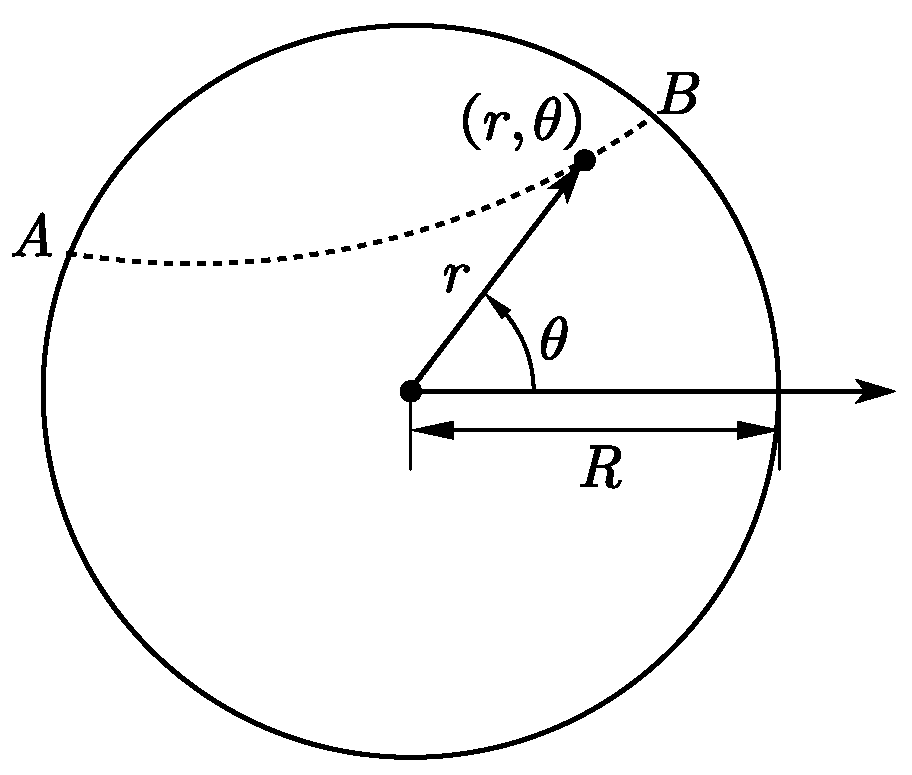
Figure 2.
Python Visualization Code.
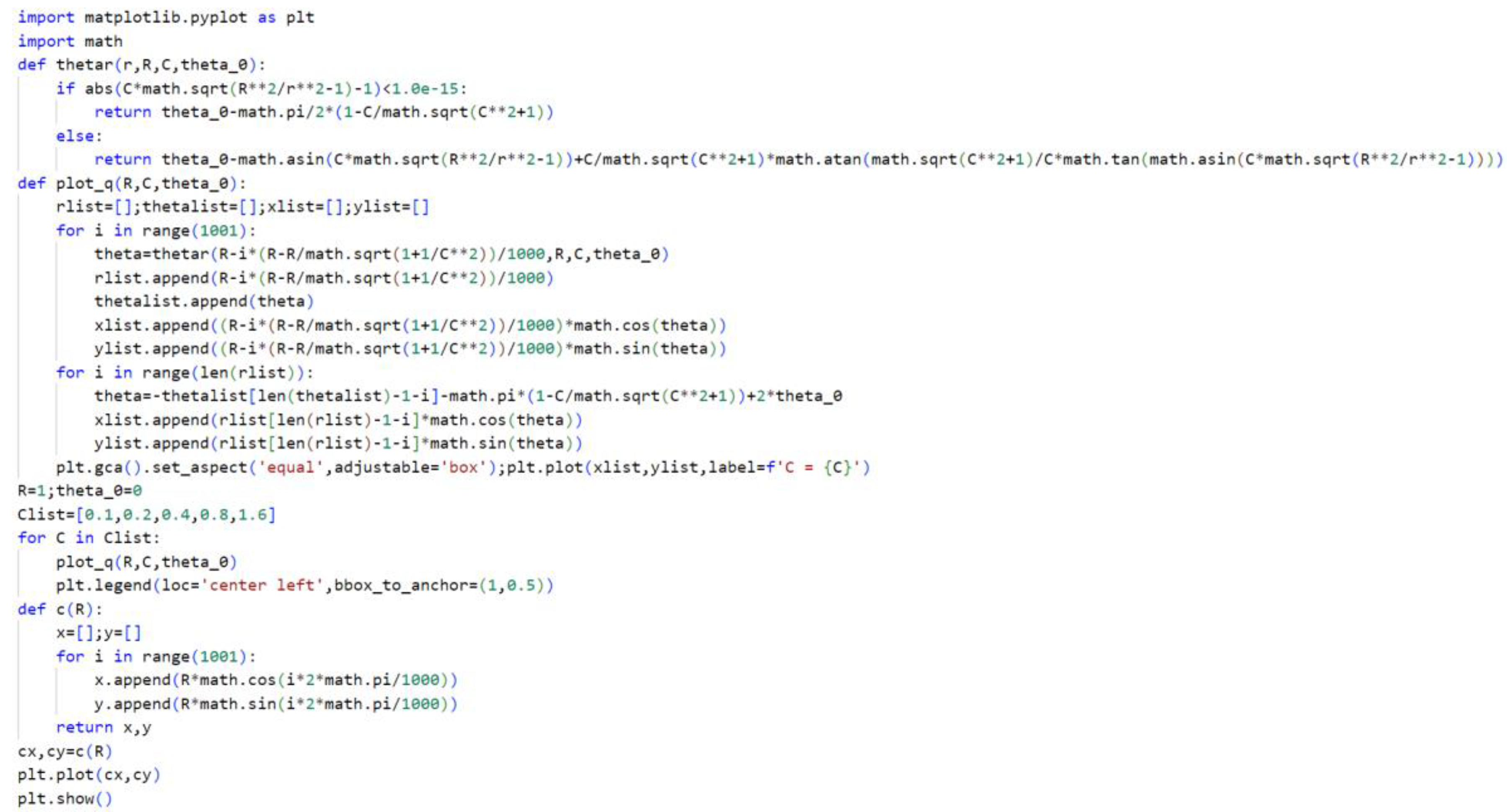
Figure 3.
Python Visualization Results.
Disclaimer/Publisher’s Note: The statements, opinions and data contained in all publications are solely those of the individual author(s) and contributor(s) and not of MDPI and/or the editor(s). MDPI and/or the editor(s) disclaim responsibility for any injury to people or property resulting from any ideas, methods, instructions or products referred to in the content. |
© 2024 by the authors. Licensee MDPI, Basel, Switzerland. This article is an open access article distributed under the terms and conditions of the Creative Commons Attribution (CC BY) license (http://creativecommons.org/licenses/by/4.0/).
Copyright: This open access article is published under a Creative Commons CC BY 4.0 license, which permit the free download, distribution, and reuse, provided that the author and preprint are cited in any reuse.


