Submitted:
22 July 2025
Posted:
22 July 2025
You are already at the latest version
Abstract
We present the idea that causal relations between system and environment can be explored through the lens of proto-cognitive properties. Basically, I propose that the notions of under-determination and self-determination can be attributed to autonomous dynamics, and that these may be measured through information metrics in the discrete case. After revising relevant theoretical concepts, I introduce some mathematical formulations in an attempt to capture these notions more formally. Then, I illustrate these ideas and exemplify the used of the formulations through a toy-experiment in the Game of Life (GoL) cellular automaton.
Keywords:
Agency
; Proto-cognition
; Causality
; Autopoiesis
; Autonomy
; Enaction
1. Introduction
Intuitively, agency can be portrayed as the capacity of a given system to determine, at least to some extent, its own behavioral trajectory (to `decide’ what to `do’). Or, in other words, to display some degree of causal decoupling from the world that both surrounds it and realizes it. Also intuitively, we often think of agency as an evolutionary trait or capacity that would have arisen at a relatively late stage, after complex adaptive properties were in place, but that, perhaps paradoxically, would be inherent to most forms of life. Unfortunately, however, beyond more or less agreed-upon intuitions, our actual scientific understanding of the underlying mechanisms supporting any real form of agency is still very unclear and has been a matter of increasing debate [1,2,3,4,5,6].
Within the framework of enactive cognitive science, insofar as life is considered to involve a teleological dimension stemming from a strive for subsistence, living beings are conceived as agents [7,8,9,10]. Roughly speaking, the idea is that the ever ongoing need for preservation in the context of dynamical environments imposes a delicate dialectic interplay, of openness to external energy sources for self-production, and of closure for self-individuation. Thus, essentially, organisms could not be blind or indifferent to their own system-environment coupling, because the risk of disintegration of their identity would entail a normative need for action, and therefore, a primeval valence on their own states, which would be irreducible to plain objective descriptions [11,12,13,14]. This idea, however, clashes with a growing literature which is more mechanistically biased and, in consequence, rather skeptical of the purported leap, especially given the necessary phenomenological association implied in this process [15,16,17,18,19,20].
Bearing this in mind, we propose a minimal approach to this problem, namely, to understand the basis of agency as the ongoing strife of a system against its environment, to determine its own behavior. More specifically, by taking a discrete perspective, here we explore the possibility of measuring, for each time step, the degree of coercion that the environment can impose over a given system, and the causal power that said system can exert upon itself.
To this end, we start by examining the problem from the perspective of selectivity, which can be understood as a causal property that determines variable degrees of response specificity (depending on the complexity of the system, the environmental circumstances and the relation between them). Starting from this basic notion, we develop the idea that although physically co-specified by environmental circumstances, system state transitions (i.e., enactions) in protocognitive systems can be characterized as more or less driven by an intrinsic `steering force’, according to the degree of causal influence that its organized sequential states can exert on its future self, under the adversarial influence coming from environmental circumstances.
This is to say that, while in fact both, the states of the environment and the system will determine the upcoming state of the system, these contributions may not always be equal (less even an exact half-and-half), therefore naturally posing the question about the dynamics of this relation. In this sense, active change may conceived as opposite to passively undergo viable transitions, in which case the dynamic persistence of the system will only depend on the environmental `good-will’. Furthermore, whereas the system’s ongoing behavior will always be determined by the environment to an extent, any minimal form of later agency will at least require a primitive capacity for self-determination, capable of overcoming the causal influence of the environment.
By self-determination, in this context, we simply mean to point out that if the influence of the system over its future state is higher than the influence of the environment, then the system can be said to be determining its future self. We posit this as a non-mental concept, purely as protocognitive traits modulating structural dynamics. As a logical counterpart, we can think of (environmental) underdetermination whenever the causal forces of the environment are not strong enough to completely specify the future of the system.
In brief, we first need an entity that is not the environment and that does not dissolve into it; an autonomous system. Secondly, we need a minimal form of asymmetry that can support the idea of agency in later stages; a latent form of agency which originates, or so we claim, at a protocognitive level as self-determination. Consequently, we deem the work presented in this manuscript to be an exploration of the protocognitive bases of agency.
The remainder of this manuscript is structured as follows: first, we review some necessary conceptual elements to present the notion of proto-cognitive self- and under-determination in terms of asymmetrical causal contributions that the system and the environment exert –in spite of their inseparable nature– over the upcoming state of the system. Then, we explore the possibility to formally approach a method for quantifying this using information measurements, and produce elemental instances that can be used in the discrete case. Later, we conceptually discuss the relation between causal determination and agency, to conclude that self-determination is a necessary, but insufficient property for agency and illustrate it through a toy-experiment in the Game of Life. Finally, we close with a brief summarizing discussion and some concluding remarks.
2. About Protocognition
There is a fundamental tension at the core of enactivism and much of the rest of cognitive science, concerning the relation between life, mind and cognition. In brief, the cause for this is the bioenactivist purported mental properties attributed to living systems, for intentionality, adaptivity or agency, in theory underpinned by their precarious nature and therefore their need for continuous gathering of energy sources for their dynamic realization [1,7,9,11,14,21].
At least from our point of view, even if this seems sensible, it also seems, as more radical positions put it, unnecessary and not properly justifiable if we limit ourselves to naturalist descriptions (i.e., by purely looking at the physical mechanisms present in their processes) [16,22,23]. It seems somehow to be a wish to endow life with meaning, or to bestow a phenomenological soul to living beings, from the valuation we as humans make from our wonder as we confront it.
In this sense, regarding the hypothetical relation between consciousness and mind, if by mind we understand someone or something that experience the very fact of its existence somehow, even if minimally; We believe that, given the current available knowledge, it is not only prudent, but also sensible to remain agnostic.
On the other hand, however, while the theoretical framework of the autopoietic approach to cognition seems to be, at least to us, the best option to build from, because of its emphasis on looking at cognitive processes as material coherences [18,23,24,25], by reducing cognition to any process of consistent structural dynamics, it conflates together properties that, from our perspective, require conceptual delimitation.
In our view, whatever life is, it is clearly something beyond autonomous dynamics and being so, it is not only fair but also correct to label the specific kind of intelligent behavior organisms exhibit as cognitive behavior, inasmuch as the processes they realize surpass by far simple system-environment coherence and consistent interpretation-response mappings [26,27,28,29,30,31]. It does not follow from this, however, that they can be said to have a mind (so sentient and purposeful control and regulation of their own states, less even of the environment in which they are embedded).
Similarly, to attribute intelligence only to living beings is excessively arbitrary. Moreover, it seems to us that, as many others have hinted or explicitly pointed out [32,33,34,35,36], this may be better understood as a mechanistic property arising spontaneously from natural laws, that leads to the formation of more intricate physico-chemical ensembles eventually leading to autonomous self-referent systems, and only much later to living systems as we know them.
As a matter of fact, a simple proof for this is the vast literature on artificial life and biologically inspired artificial intelligence, that has been able to emulate minimal cognitive-like behavior without the need of an organic motherboard, where its application in robotics is especially illustrative [37,38,39,40,41,42,43]. Few would doubt that the mechanisms underlying the behavior of the systems presented in these works give rise to intelligent behavioral patterns; whether this kind of intelligence is equivalent to that of biological systems (i.e., cognitive), we believe that the answer is no, because the different nature of the hardware will unavoidably lead to different computational specifications. In simple words, even if to some extent they may be solving the same problem –let’s say navigation–, they are poised differently; functionally speaking, the computational problem they specify isn’t entirely the same.
Along these lines, what we are suggesting is to distinguish as proto-cognitive properties the specific properties by which autonomous systems display intelligence, and by autonomy a self-referential property [44,45,46]. Therefore a particular kind of intelligent behavior which is determined by organizationally closed dynamics and which is non-mental and non-organic. Put differently, a kind of intelligence that is logically and evolutionarily prior to life, while still constrained by a recursive nature, so that the coherences that a system exhibit are not just transient or evanescent processes, but safeguarded by being encoded in the structure of the entity that remains (a minimal autonomous system).
Furthermore, the relation, or the leap between cognition as the specific kind of intelligence of living beings and the abstract notion of mind, which appears to be often the goal in cognitive science, seems somewhat premature as a research objective. For this reason, instead of moving from what we know from living beings towards more complex cognitive capacities, a better option may be trying to look for intelligent/computable properties already present before, thus underlying life.
3. Causality as Information
3.1. The Role of Selectivity
In general, systems can be described in terms of their state dynamics, so that from any particular state and set of environmental conditions, a system will transition into a second state (which in some case may be some previously visited state, or even the same as the first). This is the basic and more intuitive notion of a causal relation for how dynamical systems change.
In particular, autonomous systems belong to a specific kind of systems which are organizationally closed, meaning that their ongoing processes will recursively determine state transitions from valid (i.e., viable) states into further valid states, and where the whole set of transitions that a system can undergo without disintegrating (i.e., among valid states) is what defines its (autonomous) organization [24,44,47,48]. As such, their actions (their concatenated sequences of state-transitions) are a consequence of their own organizational constraints, together with its environmental interactions. We can express these changes in terms of structural transitions of the kind: , where and denote two consecutive states of the system, the state of the environment, and → a causal relation or mapping between them.
In this sense, enactions encode mappings, or, maybe better, they can be well represented as mappings, whereby the embodied machinery of the system specifies its upcoming states, depending on the influence from the environment. It follows from this that, as long as the autonomous system remains so, neither the system itself, nor the environment can fully specify its next state (of the system). Accordingly, we understand this process as a form of system-environment coupling that unfolds over time; the co-determination of the system’s behavioral trajectories.
This co-determination is dynamic, so much so that we know that a system can behave in the same way (i.e., perform the same state transition) even if the environmental conditions in which it is embedded are different, or, conversely, respond differently to identical external circumstances; these changes are not arbitrary and the underlying property we associate with these phenomena is the system’s selectivity. The reason is that selectivity depends on the specific structural characteristics of the system at the time of any given system-environment interaction, as this imposes limitations on the local interactions available to the parts of the system. In simple words, the physical state of the system (its shape, position, orientation, etc.) delimits/constrains what the system can perceive and do, hence making responses to the environment dependent on its own state. This is what [46] introduces as the interpretation that an autonomous system makes.
More concretely, the fact that different states of the environment elicit identical system state transition depending on the states of the system, entails that these environmental instances conform to categories, or sets of selectively equivalent environmental elements, such that:
Where every element denotes some specific environmental state that belongs to the set whereby the same state transition is enacted by the system. From now on, we will refer to these sets of causal and operationally equivalent system-environment interactions simply as equivalent categories.
We can more explicitly express an equivalent category as the set of environmental states by which the system transitions from a first state into a subsequent state , so that:
In this way, we can easily characterize the dynamic interpretations/enactions available to a minimal system through state transitions, even if every relatively complex system will presumably exhibit a high variety of transition types. Some very simple cases to illustrate these, would be:
For the first pair of transitions, the same environmental conditions will result in different subsequent states. In this case, the system’s selectivity given by different structural instantiations is the cause of diverse responses. For the second pair, however, different initial states of the system will map onto the same state under the same environmental conditions (a different state transition nonetheless). For this to happen, and assuming that , the environmental state has to be a part of both equivalent categories and even though the different states and entail . Put another way, although their responses are different, the target of their mappings is the same. The last two transitions characterize what would be a minimally recursive case, where in the absence of changes in the external conditions, the system will oscillate indefinitely between 2 states (but to exhibit a different selectivity as well). Indeed, this is a common case, for instance, in the Game of Life, where patterns such as blinkers or gliders oscillate between two configurations in the absence of perturbations.
The contrast between the cases up to this point depicts the conceptual role expressed by equivalent categories. Likewise, despite their simplicity, they are helpful to illustrate what we mean (minimally at least) by an enaction as an interpretation that is made by an autonomous system; a consistent categorization of system-environment coupled states through a coherent mapping of its own state transitions.
This implies that, on the one hand, all of the environmental conditions triggering, or co-specifying the same structural transition are, from the point of view of the system, the same enaction (insofar as maps into and is an element of the category ). On the other hand, the behavioral complexity of the system (the causal range of actions available to a systems at any time, given some state ) is then the direct consequence of the causal structure of the set of all the equivalent categories available to it, which can be better captured as a probability distribution. If, by abstracting away the effect of the environment, we consider the following open equivalent category:
Then, the sub-indices a, b, z will denote the possible future states of the system, , and , the corresponding equivalent categories, and the set of all the equivalent categories potentially available to the system in state . Further, considering that as long as the system can cope with external changes there might be as many environmental sets as the complexity of the organization of the system permits and, that the cardinality of these sets (given by the number of environmental states interpreted as equivalent) may differ greatly, then we can express the probability of the interpretation given by and enacted by a transition into a state , by the conditional probability distribution:
In this respect, an enaction is proto-cognitive, along the lines of this work, insofar as an intelligent action/response in a computational (albeit non-representational) sense. That is, a multiple realizable, intrinsically logical and consistent mapping of states, that can be represented through mathematical automated mechanisms and that does not require for the system to be sentient or alive to be performed, matching other minimal accounts characterizing cognitive-like properties exhibited by artificial systems, paradigmatically exemplified through Bittorio in [46], but described profusely in the artificial life literature, see for instance studies by [33,49,50,51,52] to mention some.
As a final note and as a preview of the following section, we shall mention that whilst enactions actively modulate the disposition of the system toward its environment, this is not the same –we argue – as saying that they actively modulate its environment. Essentially, whereas the former points to a modulation of the environment through a functional closure [53,54], the latter operation entails more sophisticated cognitive capacities, probably involving some form of symbolic or phenomenological kinds of content [16,55] that we would prefer to avoid in the current setup.
3.2. Intrinsic Information
Building on Bateson’s idea of “differences that make a difference” [56] and along similar lines about selectivity that we have examined until now, the Integrated Information Theory of Consciousness (IIT) [57,58,59,60] introduces the formal notion of intrinsic information, in order to quantify the causal effect a system, given its structure, has over itself. Roughly speaking, IIT claims that integrated information, a measure of emergent causality (often also expressed in terms of causal power), reflects the degree to which a given system intrinsically exists as such (so independent of external observation), hence, as a causally decoupled entity that becomes a phenomenological observer itself [61,62]. Technically, the goal of IIT is to provide a formal framework for quantifying consciousness, under the premise that the ontological existence of the system entails phenomenological existence [60,61], and under the broader paradigm of causal emergence [63,64].
Basically, intrinsic information is the idea that the causal sources of an irreducible system have to be self-contained. In turn, cause-effect information is the purported measure for the degree of causal-power exerted, within the system and over itself, by the very existence of its own mechanisms. This is calculated by looking at the state-transition probabilities from past- and to future states, from an incremental purview, starting from minimal mechanisms (units), up to the whole candidate system [60]. On these grounds, causality becomes fundamentally linked to selectivity, which is understood as informative (with a connotation of specificity), insofar as the state of a system and its mechanisms logically specify a finite set of possible past and future states while discarding others [59,60,65,66]. See Figure 1 for an intuitive depiction.
From there, integrated (intrinsic) information () is a second step; somehow an attempt to formally solve the combination problem [64,67] through the notion of a causally emergent unity, which would be the phenomenological experiencer. This, assuming that each of the elements of the system could have some degree of phenomenological experience on its own, but that they integrate into an irreducible physical/phenomenological mechanism. Simply put, the integration processes is a method to reveal the real system, from the many possible combinations among elements in a domain; the subsystem with the highest level of aggregation of intrinsic information.
Although the theory has gathered a lot of interest, it has also received its fair share of criticism; pointing to a lack of a principled justification for the leap from maximally integrated information to consciousness [68,69,70,71]; inconsistencies among different measures for integrated information [66]; unconvincing mechanism accounting for temporality, especially regarding the exclusion principle [72,73,74]; and the apparent impossibility of consistently apply its methods to more complex systems [75,76], among others.z In this respect, while we don’t commit to the axiomatic postulates of the IIT [59,60], nor believe there is a strong enough reason to accept the proposed causality-consciousness-existence identity, we do believe it has steered the discussion about consciousness into a scientific domain. Moreover, we believe that, as others have done by building on some of these ideas to approach particular problems, usually with respect to the linked notion of emergence [77,78], the application of the specific notion of intrinsic information may be quite fruitful in the context of our present investigation on agency, under a strict selectivity-causality interpretation. We will henceforth develop this idea.
To this end, we will make use of the concept of repertoire, by which the IIT represent the Markovian probability of every possible state transition, thereby producing two probability distributions; a cause (past-from-present) repertoire (the term ( in eq. (4)) and an effect (present-to-future) repertoire (the analog term in eq. (5)). From these we can obtain cause () and effect () information by doing:
Where the terms (past), (current) and (future) refer to the system states, considered in the context of subsequent timesteps (hence, equivalent to , and ). As mentioned, and stand for cause and effect information respectively, and for cause-effect information quantifying the causal power measurable from the system. EMD stands for the Earth Mover’s Distance [79,80] which is applied to compare cause/effect repertoires against non-intrinsically causal, unconstrained conditions (denoted by the superscript ) to provides a measure of how much the system determines its own behavior (state transitions) away from random changes or pure external determination, such as ordinary entropy decay. From these, cause-effect (intrinsic) information is obtained by taking the minimum between them: , which reflects the shared degree of causality that we can ascribe to its structure in both directions.
3.3. Cause-Effect Information in the Game of Life
Conway’s Game of Life is a cellular automaton and a zero-player game, in which the player can only choose the initial state of a grid of cells that can be alive or dead (represented by symbols like 1 and 0, or ON and OFF). Afterwards, the grid is automatically updated in discrete timesteps, by always applying the same rule to each of the cells on the grid. In simple words, the rules are the following: Reproduction: every dead cell surrounded by 3 active cells, comes to live. Overcrowding: every active cell surrounded by more than 3 active cells dies. Loneliness: Any living cell surrounded by less than 2 active cells dies. Sometimes rules and are also expressed as: living cells surrounded by 2 or 3 active cells remain alive, otherwise they die. For an illustration of different initial states and the updating rules, see Figure 2.
Moving onto our goal at hand, we will first test whether cause-effect information can be applied to approach a measure of causality (in the sense of latent agency we have discussed) by applying it to the simplest case to be found in Conway’s Game of Life; namely, a single cell with only two states and its environment, made of the surrounding 8 cells. This space, containing a central cell plus those at a Chebyshev distance equal to 1, is also known as the Moore neighborhood [82] and in this particular case can display different configurations ( for the environment). From the rules of the GoL [81,83,84] we know that a cell can only be `alive’ (active) if it is already active and there are 2 or 3 active cells in its Moore neighborhood (apart from the central self itself), otherwise, if not currently active, only if the sum of active cells in its surroundings is exactly 3. This can also be expressed as:
Where stands for the neighborhood (the Moore neighborhood minus the central cell) for a central cell () that follows a state transition . Note that the neighborhood in this case, corresponds to (the equivalent categories available to ) instead of (the actual environmental configurations), because for the central cell, the specific states do not make any difference, only their sum. And since there are: 28 combinations for , 56 combinations for and 172 combinations for the remaining non viable (i.e., deactivation) alternatives, we then have the following counts:
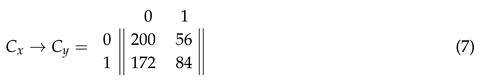
From where we can derive the probability matrices:
Now then, we can follow the IIT formulation (from equations (4)-(5)) and calculate information, by first computing cause and effect repertoires based on the current state of the cell. For the sake of the example, we will start with an active central cell at a given time t, :
Where and stand for cause and effect repertoires and the super-indices p and f refer to past and future states respectively.
We can also obtain the unconstrained (past) and (future) probability distributions through direct counting. First, by considering that represents the probabilities of the past state of the system without any knowledge of its current state (transition into if looking at the transition counts in (Section 3.3)), so unconstrained by it, which logically entail a uniform distribution.
Similarly, represents the probabilities of the future state of the system without any causal input from (or, again, unconstrained by) , which is the same as not having any knowledge about the current state of the system, hence a vertical sum of the elements in the transition matrix from Equation (Section 3.3).
Put differently, whereas the unconstrained past is formalized as a simple homogeneous distribution (assuming unconstrained outputs), the unconstrained future distribution is taken as independent of the current state of the system, although still dependent on its causal structure (i.e., as a system with unconstrained inputs). In this sense, the unconstrained repertoires represent the marginal probability mass in both directions. Formally, this can be concretely expressed as:
Moving on, cause and effect information are computed by comparing cause and effect repertoires against their unconstrained () reciprocal repertoires. Information is calculated in terms of distance (difference) between the compared distributions, using the EMD:
Thus . Which, leaving aside hypothetical connections to phenomenological properties of any kind, is basically an expression of the fact that our knowledge about the ON state of a single cell is informative to the extent it gives us an insight into its past and future states. From this it follows that, when put in terms of causality, cause-effect information may be interpreted as the constraints that the state of the ON cell places upon its state transitions, hence the degree of self-determination with respect to its environment (i.e., the rest of the Moore neighborhood, within the context of our example).
Then, by repeating the process for we obtain:
Then making . This, as might be expected, shows that active cells on the grid have a slight higher causal power () than non-active cells, which is reasonable considering the amount of transitions leading to ON and OFF states by the dynamics of the Game of Life.
As a recapitulation from our toy case example we can highlight some simple things; first, information is low, because from only knowing the value of one cell we don’t really have a lot of information about its past or future state, as this depends mostly on its neighborhood. Second, the highest and lowest information values correspond to the cause information for an active cell () and () respectively, meaning that in the context of the GoL, single active cells are the most informative and, conversely, non-active cells provide the least information when looking backwards, which fits in with what we know about its dynamics as well. Lastly, do note that the fact that the value of effect information is the same in both cases is not due to identical effect repertoires, but a result of the geometrical equivalent distance with respect to the unconstrained probability distribution for future states. Although these simple points may not really significant, they are helpful to emphasize the possibility of causal interpretation from the application of the IIT formulations, without further conceptual escalation into more uncertain matters.
As a final note in this respect, it may be important to mention that there is no need for further integration calculations, because the object of study we have selected (a single cell on the grid) is, by definition and by the dynamics of the GoL, the minimal possible (therefore irreducible) case. This is somehow similar to the notion of monad from IIT 4.0 [60].
4. An Alternative Approach to Information
In this section, we propose to apply the ideas on intrinsic information we have reviewed so far, to the concept of enaction. In particular, we argue for a conceptual switch from a single state-based unit, to an enaction (in the minimal sense used in Varela et al. [46]) as the object of examination and, hence, as the source of information. Along these lines, regarding the conceptual asymmetry required for agency, we propose to shift the traditional enactivist view of an agent as one that controls its environment, to one that controls its own upcoming states, in spite of the influence of the environment. We shall briefly discuss this now.
As noted above, the subjective interpretational dimension of autonomous systems stems from two intertwined features; their dynamic structural selectivity and their organizationally coherent state transitions. This is what underpins their proto-cognitive capacity for adaptation and, therefore, propels their consistent distinctions and actions. Neither selectivity, nor adaptivity, have a mental or even cognitive connotation in this context, of course, but they serve as mechanistic concepts to understand the dynamic evolution of a particular kind of system.
The reason that cognitive theories (or other approaches to cognitive phenomena, such as the IIT) stress the importance of selectivity is because, any reliable cognitive distinction made by a system will require a stable pattern of structural change that correlates with specific traits of the environment, as otherwise, in the absence of this minimal form of consistency, there would be no cognition and no observer whatsoever. Put differently, selectivity plays the role of a primordial mechanism, based only on the physical properties of a system, by which it can incrementally develop intrinsic regularities that correlate with the environment.
It follows from this, or at least so we argue, that in order to correctly account for what a proto-cognitive system does, we need to understand what it interprets, and vice-versa, in terms of enactions. Enactions, in effect, are proto-cognitive irreducible events, they merge the causal role of the system and the environment into a unique distinction-action operation which is structurally realized. This introduces two necessary changes to the information measurements we have described until now; first, it becomes necessary to determine the different causal contributions of system and environment to an enaction, for this, a good measure of information should provide us an insight on their causal weights. Secondly, given that enactions encompass an operation of structural transformation including two states, we believe that a better approach would be to characterize it as a process, to stress the point that, as such, it brings a minimal, inceptive temporal component that can not be discarded. More in detail, we may say that:
State transitions in autonomous organizations are not only causally related to action, but to both; perception and action as a single operation that is a material manifestation of some system-environment coherence (i.e., enactions). Enactions involve (in the minimal discrete case) a pair of system states, but also an environmental interaction that impels certain dynamics, and a consistent mapping function between them, which is encoded in the structure of the system itself. This is a process, instead of a state, therefore extended —even if minimally, in time.
Information-wise, autonomous systems are closed, or self-referential, where information has the connotation of instruction or specification [85,86]. In this sense, we can distinguish between two types of causal inputs, namely, one from the same system and one from the environment, which has to be interpreted by the system. The latter plays an equivalent functional role, but it depends on the selectivity of the system, it does not determine it.
Given that organizationally closed systems can only computationally (i.e., by means of mechanisms) specify their own states, whatever else they influence or are influenced by-, because of their material states and changes may be certainly causal, but it is not a proto-cognitive feature of the system, because information is confined to the organization itself. This is why we suggest that autonomous systems may actively control their upcoming states, but not those of their environment without representations; because they do not have any kind of access to what is beyond their own existence as a system. Similarly, the causal influence of the environment over the system only becomes a protocognitive feature once incorporated in its recursive dynamics.
The consistent mapping between the system/environment states and the resulting state of the system is the most basic form of coherence displayed continuously by an autonomous organization, however, for any primitive form of agency to arise, there must be some fundamental form of asymmetry between system and environment’s causal forces, by which, even if transiently, the system can overthrow the effect of the environment to some extent. Inasmuch as these mappings are not univocal, given the ongoing struggle between system and environment influences, they may be represented in a space which is better expressed through probability distributions.
At a proto-cognitive level, a primitive form of agency gives rise to a causal dissociation from the environment and that amplifies its degree of influence upon it self. From now on, we will refer to the former as environmental under-determination, and to the latter as causal self-determination, both underlying the operation of the system. We refer to this particular quality as being latent, to stress the fact that the exploitation of this increase of self- and under-determination will require higher order, representational or phenomenological properties to render such actions/responses meaningful to the a real agent.
In concrete, we will move away from the past-current-future view by examining only the two states of the system involved in an enaction. By recalling the formulation of repertoires from eqs. (4) and (5), we can express a single causal direction as:
Here, corresponds to the effect repertoire, which, while conceptually different, is formally the same as in eq. (5) (X represent the specific state of ). The notation has been modified to avoid unnecessary confusions further on.
In order to investigate possible asymmetric contributions, we need to conceptually delimit system-system and environment-system influences and try to formally disentangle them, for quantification.
Tentative starting points could have been the enactivist notion of intentional (in the sense of directedness) action [7,87] or interactional asymmetry [1,88]. However, we would like to avoid cognitive properties of higher order than the ones exhibited by minimal autonomous systems and a theoretical framework in which the fundamental asymmetry is characterized as system-to-environment. Essentially, this would depict a notion of agency that seems unfeasible, either without representational capacities (e.g., requiring a model of the world) or some minimal phenomenological attributions, by which some form of ex nihilo meaningful sense-making could drive the system modulation of the environment in accordance to its needs [8,15,16,18,74], which would implicitly entail that even minimal manifestations of agency are logically dependent on consciousness, or exclusive of higher order cognitive properties.
Being thus, we will leave aside from our constructs the future-environment component and incorporate the notion of asymmetry only in terms of the influence that the environment has over the system, in order to enable a formal method to later examine it in opposition to that of the system upon itself. To this end, we will introduce a second repertoire:
Where the term refers to the equivalent categories available to the system, to the state of the same system and X to some specific state. The argument is because is a weighted mapping of the equivalent category defined by and . Thus, it expresses the probability of the next state of the system, considering the interpretations that the system can make from the conditions of the environment. In other words, this is the effect of the environment over the system, given its particular structural selectivity; the proto-cognitive interpretation of the environment that the system makes.
Having both repertoires, we are now provided with the elements to examine causality by quantifying it in terms of information. Along these lines, the first step will be to compute the entropy of these individual repertoires, where entropy is defined as:
Entropy, in this context, can be understood as an indicator of causality, or maybe better, an indicator of the latent degree of causality allowed.
Later, along the lines of intrinsic information, we will make use of the EMD metric to compute the distance of the repertoires against ideal conditions (highest and lowest entropy cases respectively) and then between them. In this case, given that the Earth Mover’s Distance is a commutative metric, distance would reflect how far they are from each other, although without indicating which of the repertoires is causally stronger than the other. Being thus, we will apply EMD measurements three times: one to compare the environment-system influence () against a uniform distribution (which in theory would be the one more exploitable by a system). Another to compare the system-system repertoire () against a totally determined distribution, and a last one to measure the distance between the repertoires themselves, hence hinting at how stronger the causality is from one with respect to the other, which along with the rest of the measurements will give us a relatively good idea of the general picture. We will develop these ideas in detail in the next section.
5. Coming Back to GoL
5.1. The Minimal Case
Coming back to the minimal case of a single cell in the Game of Life and following from the descriptions given in the previous section, we can note that, whereas the objective environmental states conform a set encompassing all the possible configurations that the 8 cells in a neighborhood of the central cell can instantiate, the equivalent sets that the central cell can distinguish are only 3 and given by their sums. Hence, we can group these cases and get the number of combinations by applying a simple combination formula:
From where we obtain: and for transitions into active cells (so that and for the remaining cases. The symbol q refers to the rest of the sums: , whereby only transitions into non-active states are generated. From this, we can systematize transitions in terms of enactions as in Table 1.
We have previously examined this system on its own, hence, we now need to derive the possible transitions as a function of the environment (i.e., the environment-system component of the coupling). This is presented in Table 2.
After this, by making use of Table 2, we finally are in position to derive the environmental causal components as probability distributions (repertoires). As it can be inferred, the only environmental category that enables some degree of causal freedom to the system is , because for all cases in which the sum of the surroundings cells is 3, the subsequent state of the single cell in the centre will unavoidably be ON (), independently of its own state. Conversely, for any other case, the subsequent state of the single cell at hand will be OFF (). This exemplifies different degrees of causal environment-state determination and can be related to the entropy of these distributions (in bits):
Hence, illustrating the two extreme cases; the former shows how for some environmental categories, the selectivity of the coupling allows a degree of environmental under-determination that may be exploited by the system. Conversely, the other two cases totally preclude any kind of effective system-system determination, due to the strength of the environmental influence. In both cases the system there is a component of self-determination, the key difference is that in the latter case (for ) what actually determines the state transition (so the enaction) is the state of the system (; it is the difference that makes a difference.
The entropy of the correspondent distributions given by can be calculated accordingly:
Entropy, as an indicator of the uncertainty of the outcome given by the probability distribution (as it can be seen from the extreme cases of the entropies resulting from the environmental repertoires) has two important interpretations: Regarding the environment, as we have seen, entropy tell us the degree to which a system might be able to exert causal effects in its own future states, if any at all.
This seems intuitively easier to understand from the other way around (system-to-system); in this case, a probability distribution with very uncertain outcomes (like one close to a uniform distribution), would probably provide less chances for a system to influence its future states. Because, for this to occur, the system needs not only to encounter itself in circumstances of environmental under-determination, but also to be capable of exploiting them, and the more focused tendencies will result in lower entropy values. In this sense, at least generally speaking, likely ideal conditions would be high environmental interpretability and entropy, along with focused, so low, system entropy. In simple words; to have as many options as possible, but to strongly pursue only a few (hopefully one).
Given that totally determined and uniform probability distributions are the extreme cases for lowest and highest entropy values respectively, and considering that we’d like for the system-system and the environment-system cases to be as close as possible to said type of distributions; we can apply a distance information measure to see how far the actual repertoires are from the ideal ones, making use of the Earth Mover’s Distance measure [79,80].
We have decided to use EMD mainly for two reasons: first, other comparative information measures we approached, such as KL-divergence (which was our first option, due to its lack of geometrical symmetry and its non-commutativity) or Mutual Information (for which there is a vast literature regarding causality), suffer too much from multiple zero values, something that can frequently occur in this context, making them computationally unsuitable. Second, especially with respect to the comparison against ideal conditions, EMD gives a fairly intuitive interpretation in terms of how much work, or energy, would be needed to change some particular repertoire into the desired probability distributions.
Being so, for the first environmental case () we obtain:
Where stands for the discrete uniform distribution and for the difference to the ideal case (how far from total under-determination). Then, for the externally determined cases ( and we get:
Which, given the simplicity of the example at hand, can be interpreted directly like the ideal environment-system condition (hence, eventually allowing some form of cognitive agency) and the opposite scenario, respectively. It follows that, the lower the entropy value, the higher the degree of under-determination and the chances of effective self-determination. In other words, captures the degree to which environmental conditions constrain the future of the system, or how entangled the response of the system is with respect to the interpretation it does from the environment1.
Do note that, although the contrary is also true (the higher the distance value, the smaller the space for the system to act on its own), the value of this metric is not something fixed (, for example) because, given the EMD algorithm, it depends significantly on two features, the number of possible elements and the distance among the elements within the distributions themselves. This is actually particularly relevant for the comparisons of the system-system repertoires, as the totally determined system-system future state will be represented by one state being one, and the remaining being zero. Thus, the position of the value for which within the probability distribution will matter, insofar as it represents a difference between that state and the rest of the possible states of the system.
We reckon, however, that it is not necessary to incur an unfeasible number of calculations (like power-set permutations or something alike), but only to compare the repertoire against the totally self-determined case, in which the highest probability within the repertoire is taken as the only possible (i.e.,; , while all remaining elements are made zero). Note that this represents the minimum value for such a change to be possible and that it will be necessarily higher, and therefore less likely, for any other case, like, for example, a hypothetical one arising from intrinsic motivations corresponding to some other option.
Accordingly, we will denote this construction as (focused) and as the distance between the repertoire and . For the system repertoires we obtain:
Which basically indicate the difference (conceivable in terms of energy/work) that would be required to transform the state of the system into the ideal, most focused case possible (); simply put, the distance to the highest degree of self-determination.
Unlike the previous case (), for the interpretation may be a bit less straightforward; on the one hand, it provides a simple measure of the degree of protocognitive self-determination. On the other hand, however, it does not seem to leave a space for a phenomenological system to ingrain higher order motivations, at this at this level. It may be the case that the ideal distribution is far from , but also from , and therefore that an agent could be capable of meaningfully acting under particular conditions in which, for instance, a few options concentrate most of the probability mass, for which a slight difference from mechanisms, hypothetically amenable to phenomenological distinctions, could make a causally strong-enough difference, more along the lines of second order cybernetics [89]. Anyhow, this requires further elaboration that is out of the scope of this work, but we will briefly expand on this in the Discussion section.
Finally, as we anticipated, we can also apply EMD to compare between the repertoires. Given that we know that for and there’s no possible under-determination, we will just examine the case:
Once again, this can be easily related to the previous results and our knowledge of the minimal dynamics of the isolated cell in the GoL. And indeed, as expected from the above EMD comparisons, we see that the distance between the repertoire for and is less than for versus .
Whereas the numerical results we have seen until now are quite evident themselves, this will not always be the case, especially as the complexity of the systems being examined increases. The purpose of this work has been to showcase the minimal possible case in the most intuitive fashion, to develop a first assessment for these methods. In the following section, we will explore a more complex case, from the dynamics of emergent patterns in the Game of Life. The scope, nevertheless, remains the same and we will avoid unnecessary complications as much as possible.
5.2. A More Complex Case: Structural Transitions
Emergent patterns in GoL have different probabilities of maintaining their structural states, transitioning into new structures (as instances of the same organization), or disintegrating. All of these are consequences of the spontaneous dynamics of their interaction with the environment as emergent units, which has proven to be a good ground for toy models of autopoiesis and autonomy [84,90,91,92,93]. Because of this, and in order to further test our intuitions, we analyzed transitions among a set of different GoL patterns and applied the same measurements that we used for a single cell (the patterns we will discuss are presented in Figure 3).
To understand the transitioning behavior, we simulated all the possible transitions that these patterns could undergo (from to cases, depending on the number of environmental cells) and searched for occurrences of the same patterns in the grid codomain after transitions (i.e., the following time step). Firstly, the system and environment repertoires were built by computing the probability distributions from the counts. Then, I calculated the entropy of each individual distribution, while making comparisons between them using the EMD as we did for the single cell. Given the data of the transition counts, obtaining the system-system repertoires and entropy is quite a direct process. The results of these procedures are displayed in Table 3.
Further, to obtain a measure of the effect of the environment over the system, following the steps from the previous section, We first separated the possible state-environmental categories combinations, to then look for the subsets of these equivalent categories (the elements within each ) that could have been interpreted differently if the state of the system itself were to be different.
Thus, given some enaction , where , we want to find at least a set , for which an arbitrary (viable) state , under the same environmental circumstances , could have produced another enaction: , where and , and where the set describes all alternative interpretations for each of the n states of the system.
Furthermore, if there are no alternative transitions to some when varying the external conditions, then is being determined only by the environmental perturbation, because the system does not have a range of interpretation availability; the only possible transition is the one being examined. Therefore, we would like to find cases, where the recursive dynamics of the system will trigger divergent transitions for identical environmental conditions (by interpreting them as an element of a different equivalent category). Hence, where identical objective environmental states are not locally (i.e., behaviorally) equivalent and viceversa.
For instance, if we start by looking at the transitions between the 2 canonical states of the glider (denoted as `gliderA’ and `gliderB’ in Figure 3, and respectively from now on), we find that, for there is just one alternative () accounting only for 32 cases of a total of 32,800. Leading to .
Similarly, for the opposite state transition , we get: , which although higher due to more structural alternatives (including a recurrent case to ()), is still quite low compared to the entropy values of repertoires presented in Table 3. This, of course, is to be expected from a toy scenario such as GoL, especially taking into account the low level of complexity of the patterns at hand.
Ideally, as we have discussed above, we would like to encounter an entropy value as close to zero as possible for the repertoire (i.e., strongly focused) and, conversely, the highest possible for the entropy of the repertoire, close to a uniform distribution, which would imply that the system has as many responses for a given environmental case, as viable states. With this in mind, we would to examine cases along these lines.
As is visible from the results in Table 4, there is a general tendency towards lower values from environment-system entropy measures, along the lines we have discussed until now. As a matter of fact, the only case in which (i.e., that the environment-system potential influence is lower than than that of the reciprocal system-system influence), is for the tetrisL pattern, when transitioning into a blinker.
This does not mean that this GoL emergent pattern can display agency in the cognitive connotation of the term, nor that it is choosing to undergo that specific state-transition, which would presumably require representational, phenomenological or some other kind of properties which are alien to the mechanisms of minimal autonomous systems. Nevertheless, the point that we would like to make here is that there are more complex cases in which the system degree of causal power can take advantage of the under-determined milieu of the environment and specify its own upcoming state; its future state is mainly determined by its present state, hence the system exerts a protocognitive self-determination.
6. Conclusions and Further Work
We have proposed a slightly different approach to the problem of agency in the context of enactive cognitive science [1,5,94]; strictly in terms of causal influences, where the ongoing structural changes of a coupled system-environment are not assumed as uniform, therefore portraying an asymmetrical and dynamic account of system-environment co-determined behavior.
Following views of cognition that had cast doubts on the unspecified mechanisms by which traditional enactive hold the assumption of an ex nihilo phenomenological origin of adaptivity and agency [16,17,19,22,23,93,95], we have analytically explored the feasibility of a mechanistic source for a causal asymmetry between autonomous systems and environment.
Indeed, some of these accounts actually argue for an opposite belief; that autonomous systems are not capable of breaking from a physically based, causal symmetry (unless we invoke higher order cognitive processes, mediated by language or culture). We have described here, though, how this kind of asymmetry may be viable, without recurring to any kind of mental properties, representational or phenomenological, hence, in pure proto-cognitive terms.
Specifically, this would be the capacity of the system to specify its own future state of the system to a higher extent than environmental conditions causally influence it (the system upcoming state). We have the term under-determination to refer to the phenomenon, by which, the interpretation of the environmental conditions, given by the specific selectivity of the system, permits a broader range of system’s actions, corresponding to more a balanced of the probability mass. Conversely, we have used the term self-determination to refer to the causal power that the system exerts upon its own future state and, following from these, proposed that an incipient protocognitive form of agency occurs whenever the degree of self-determination overcomes the under-determined causal contribution from the environment.
It is our impression that, in this sense, an important feature regarding the origin of agency, insofar as a minimal property enabling self-determination, can be traced (logically and evolutionarily) to the mechanistic dynamics of autonomous organizations, hence prior to biological or mental phenomena. Along these lines, we suggest that this form of protocognitive basal agency is a necessary, albeit not sufficient condition for the development of observer-based notions of agency [5,89,96,97].
Further, in pure proto-cognitive terms (i.e., insofar as non mental, autonomous intelligent behavior), the specific self-persisting nature of autonomous systems would allow them to recurrently undergo multiple discontinuous events of latent agency, even if this is statistically uncommon as we saw in the latter case of GoL examples. This matches well with the proposed idea of flickering emergence [78], whereby a system may be conceived to be discontinuously emergent instead of in a binary emergent/non-emergent fashion. In the case presented here, this would be translated as a protocognitive capacity, sporadically enabling self-determination, only when some (environmental and systemic) conditions can be met.
Regarding limitations, while we have developed some formulations that can be applied in minimal discrete cases, we acknowledge that a more general formulation instead of a series of point-wise comparisons would be a great advance for understanding behavioral trajectories. Similarly, while cellular automaton may present a good terrain for clarity’s sake, it definitely put too strict limits on the exhibited behavior of the systems we would like to observe.
A more important issue we should address is the two-folded mapping we have developed. In this respect, we reckon that the first half of the overall idea is more robust than the second. More specifically, while under-determination as a consequence of an expanded set of available interpretations of environmental perturbations, makes it seemingly easier to define an ideal metric for comparison (the uniform distribution), the inverse case is not that evident. In fact, the purported requirement for its exploitation, that is, the statistical concentration of its potential responses into one, may be counterproductive when considered in the context of later exploitation by more complex systems. Put another way, it could well be the opposite case (i.e., a highly underdetermined output), or some kind of in-between concentration of the probability mass in a few alternatives, would facilitate exploitation in certain scenarios
Furthermore, this take us to a different but common conundrum, namely; while seemingly compatible, under careful consideration, self-determination and a more intuitive form of agency (i.e., motivation-based or decision-making-like) seem to be rather contradictory, insofar as the mechanisms enabling the former should preclude the latter.
Autonomous organizations, in this respect, operate as subordinating mechanisms by which the otherwise much wider domain of responses of every component becomes narrowed in order to produce increasingly coordinated global transitions (autopoiesis being the strongest case in this regard) [55,98]. Nevertheless, this type of ideal system, in which every action is realized automatically, would not leave space for decision making of any kind. Further work in this direction is necessary and could well include theories on hypothetical non-computational properties [5,51,95,99,100,101].
Along the lines of protocognitive capacities, more interesting further work could involve the exploration of under- and self-determination in small groups of minimal systems, first, to see whether they are capable of more effective environmental influence regulation and, more importantly, to explore the possibility of some form of collective exploitation for local/individual under-determination. In this case, group responses would promote locally favorable environmental conditions for some members, that could steer the global response of the whole group [102,103].
Moreover, this could provide insights into the ongoing strive between causal influences in top-down and bottom-up directions (i.e., system versus and components). Measurements of fluctuations of causal information in these different levels could be applied to intermediate cases of aggregation, like the Physalia physalis (Portuguese man-of-war) or other colonies, in which it is not clear whether the behavioral responses of the global system is really emergent, the result of the local individual responses, or some middle ground combination of them.
The incorporation of current developments in metrics of emergence [77,78,104,105] could certainly give us an important insight, and provide us with better and more detailed information about the dynamics of under- and self-determination. Notwithstanding, we believe that such information would still describe phenomena at the same level of analysis that we have done here, thus not yet of the kind that we expect for an account of agency in a fully cognitive sense. Having said that, we reckon that this would be the most productive branch for conceptual work, insofar as it could constitute a solid grounding for more exhaustive investigations and, in particular, because it may be the case that the dynamics of a system under sustained self-determined states will exhibit unexpected or unforeseen properties.
A final remark regarding limitations and further work: Although we have used the Game of Life as our ground for testing and building proof of concepts. This strategy, however, has a fundamental limitation that may have become evident as this point, namely, that the dynamics of the discrete state-transitions are too constrictive. Indeed, the core of the issue goes beyond the simultaneous update of the whole grid, but deeper, to the implicit idea that cognitive (and protocognitive) properties somehow have to mirror, or reproduce, the temporal logic that enables them.
What is more, it may be argued that many conceptual problems of enactivism can be traced back to a lack of a mechanistic explanation for the temporal dimension of cognition [93,106,107]. To some extent, this relates to ideas from the Free Energy Principle (FEP) and predictive processing, according to which an essential requirement for motivated behavior is the generation of a temporally deep model of the world [30,74,108,109,110]. In this sense, real agency seems to be unavoidably tied to phenomenology and to some sort of cognitive temporal handling of time, which may indicate that more complex protocognitive mechanisms rely on non-linear temporal dynamics.
Funding
This research received no external funding.
Data Availability Statement
The datasets presented in this article are not readily available due to technical limitations (large size of respective files). Requests to access the datasets should be directed to f.rodriguez-vergara@sussex.ac.uk. The original code for the datasets presented in the study are openly available at: https://github.com/dinosaurioinvisible/gol
Conflicts of Interest
The authors declare no conflicts of interest.
References
- Di Paolo, E.; Burhmann, T.; Barandarian, X. Sensorimotor Life: An enactive proposal; Oxford University Press, 2017.
- Potter, H.; Mitchell, K. Naturalasing agent causation. Entropy 2022, 24. [Google Scholar] [CrossRef]
- Baltieri, M.; Iizuka, H.; Witkowsi, O.; Sinapayen, L.; Suzuki, K. Hybrid Life: Integrating biological, artificial, and cognitive systems. WIREs Cognitive Science 2023, e1662. [Google Scholar] [CrossRef]
- Biehl, M.; Virgo, N. Interpreting systems as solving POMDPs: a step towards a formal understanding of agency. In Buckley, C.L., et al. Active Inference. IWAI 2022, Communications in Computer and Information Science, vol 1721.; Springer, Cham, 2023. [CrossRef]
- Froese, T. Irruption Theory: A Novel Conceptualization of the Enactive Account of Motivated Activity. Entropy 2023, 25, 748. [Google Scholar] [CrossRef]
- Seifert, G.; Sealander, A.; Marzen, S.; Levin, M. From reinforcement learning to agency: Frameworks for understanding basal cognition. BioSystems 2024, 235, 105107. [Google Scholar] [CrossRef]
- Weber, A.; Varela, F. Life after Kant: Natural purposes and the autopoietic foundations of biological individuality. Phenomenology and the Cognitive Sciences 2002, 1, 97–125. [Google Scholar] [CrossRef]
- Villalobos, M.; Ward, D. lived experience and cognitive science. Reappraising enactivism’s Jonasian turn. Constructivist Foundations 2016, 11, 802–831. [Google Scholar]
- Di Paolo, E.A.; Thompson, E.; Beer, R.D. Laying down a forking path: Tensions between enaction and the free energy principle. Philosophy and the Mind Sciences 2022, 3. [Google Scholar] [CrossRef]
- Rostowski, A. Freedom: An enactive possibility. Human Affairs 2022, 32, 427–438. [Google Scholar] [CrossRef]
- Thompson, E. Mind in life: biology, phenomenology and the sciences of mind; Cambridge MA: Harvard University Press, 2007. [Google Scholar]
- Kirchhoff, M.; Froese, T. Where There is Life There is Mind: In Support of a Strong Life-Mind Continuity Thesis. Entropy 2017, 19, 169. [Google Scholar] [CrossRef]
- Gallagher, S. 4E Cognition. Historical Roots, Key Concepts, and Central Issues. In Newen, A.; Bruin, L. de; Gallagher, S. (ed.), The Handbook of 4E Cognition; Oxford University Press: Oxford, 2018. [Google Scholar]
- Froese, T. To Understand the Origin of Life We Must First Understand the Role of Normativity. Biosemiotics 2021, 14, 657–663. [Google Scholar] [CrossRef]
- Hutto, D.; Myin, E. Radicalizing Enactivism. Basic minds without content.; MIT Press, 2012.
- Hutto, D.; Myin, E. Evolving Enactivism. Basic Minds Meet Content; MIT Press, 2017.
- Abramova, K.; Villalobos, M. The apparent (Ur-)Intentionality of Living Beings and the Game of Content. Philosophia 2015, 43, 651–668. [Google Scholar] [CrossRef]
- Villalobos, M.; Silverman, D. Extended functionalism, radical enactivism and the autopoietic theory of cognition: prospects for a full revolution in cognitive science. Phenomenology and the Cognitive Sciences 2018, 17, 719–739. [Google Scholar] [CrossRef]
- Tallis, R. Freedom: An impossible reality; Agenda Publishing Limited, 2021.
- Rodriguez, F. Inside looking out? Autonomy, phenomenological experience and integrated information. In Proceedings of the ALIFE 2022: The 2022 conference on artificial life. MIT Press; 2022. [Google Scholar]
- Di Paolo, E. Autopoiesis, adaptivity, teleology, agency. Phenomenology and the Cognitive Sciences 2005, 4, 429–452. [Google Scholar] [CrossRef]
- Maturana, H. Ultrastability... autopoiesis? Reflective response to Tom Froese and John Stewart. Cybernetics and Human Knowing 2011, 18, 143–152. [Google Scholar]
- Villalobos, M.; Palacios, S. Autopoietic theory, enactivism, and their incommensurable marks of the cognitive. Synthese 2021, 198, 571–587. [Google Scholar] [CrossRef]
- Maturana, H.; Varela, F. Autopoiesis: the organization of the living. [De maquinas y seres vivos. Autopoiesis: la organizacion de lo vivo]. 7th edition from 1994.; Editorial Universitaria, 1973.
- Maturana, H.; Varela, F. The tree of knowledge: The biological roots of human understanding; New Science Library/Shambhala Publications., 1987.
- Lyon, P. The biogenic approach to cognition. Cognitive Processing 2006, 7, 11–29. [Google Scholar] [CrossRef]
- Allen, M.; Friston, K. From cognitivism to autopoiesis: towards a computational framework for the embodied mind. Synthese 2018, 195, 2459–2482. [Google Scholar] [CrossRef]
- Lyon, P.; Keijzer, F.; Arendt, D.; Levin, M. Reframing cognition: getting down to biological basics. Phil. Trans. R. Soc. B 2021, 376, 20190750. [Google Scholar] [CrossRef]
- Levin, M.; Keijzer, F.; Lyon, P.; Arendt, D. Uncovering cognitive similarities and differences, conservation and innovation. Phil. Trans. R. Soc. B 2021, 376, 20200458. [Google Scholar] [CrossRef]
- Wiese, W.; Friston, K. Examining the Continuity between Life and Mind: Is There a Continuity between Autopoietic Intentionality and Representationality? Philosophies 2021, 6. [Google Scholar] [CrossRef]
- Lyon, P.; Cheng, K. Basal cognition: shifting the center of gravity (again). Animal Cognition 2023, 26, 1743–1750. [Google Scholar] [CrossRef]
- Newell, A.; Simon, H.A. Computer Science asEmpirical Inquiry: Symbols and Search. Communications of the ACM 1976, 19, 113–126. [Google Scholar] [CrossRef]
- Hanczyz, M.; Ikegami, T. Chemical basis for minimal cognition. Artificial Life 2010, 16, 233–243. [Google Scholar] [CrossRef]
- McGregor, S.; Virgo, N. Life and its Close Relatives. In Proceedings of the Kampis, G., Karsai, I., Szathmáry, E. (eds) Advances in Artificial Life. Darwin Meets von Neumann. ECAL 2009. Lecture Notes in Computer Science(), vol 5778. Springer, Berlin, Heidelberg, 2011.
- Dueñas-Díez, M.; Perez-Mercader, J. How Chemistry Computes: Language Recognition by Non-Biochemical Chemical Automata. From Finite Automata to Turing Machines. iScience 2019, 19, 514–526. [Google Scholar] [CrossRef]
- Egbert, M.; Hanczyc, M.M.; Harvey, I.; Virgo, N.; Parke, E.C.; Froese, T.; Sayama8, H.; Penn, A.S.; Bartlett, S. Behaviour and the Origin of Organisms. Origins of Life and Evolution of Biospheres 2023, 53, 87–112. [Google Scholar] [CrossRef]
- Brooks, R. Intelligence without representation. Artificial Intelligence 1991, 47, 139–159. [Google Scholar] [CrossRef]
- Cliff, D.; Husbands, P.; Harvey, I. Explorations in Evolutionary Robotics. Adaptive Behavior 1993, 2, 73–110. [Google Scholar] [CrossRef]
- Beer, R. The dynamics of adaptive behavior: A research program. Artificial Intelligence 1997, 20, 257–289. [Google Scholar] [CrossRef]
- Quinn, M. Evolving Communication without Dedicated Communication Channels. In Proceedings of the Kelemen, J., Sosík, P. (eds) Advances in Artificial Life. ECAL 2001. Lecture Notes in Computer Science(), vol 2159. Springer, Berlin, Heidelberg, 2001. [CrossRef]
- Baddeley, B.; Graham, P.; Husbands, P.; Philippides, A. A Model of Ant Route Navigation Driven by Scene Familiarity. PLoS Computational Biology 2012, 8, e1002336. [Google Scholar] [CrossRef]
- Egbert, M.; Barandiaran, X. Modeling habits as self-sustaining patterns of sensorimotor behavior. Frontiers in Human Neuroscience 2014, 8, 1–15. [Google Scholar] [CrossRef]
- Tani, J. Exploring Robotics Minds. Actions, Symbols, and Consciousness as Self-Organizing Dynamic Phenomena; Oxford University Press, 2017.
- Varela, F. Principles of Biological Autonomy; North Holland, 1979.
- Varela, F. Two Principles for Self-Organization. In Ulrich, H., Probst, G.J.B. (eds.) Self-Organization and Management of Social Systems; Springer Series on Synergetics, vol 26. Springer, Berlin, Heidelberg., 1984.
- Varela, F.; Thompson, E.; Rosch, E. The embodied mind: Cognitive science and human experience; The MIT Press, 1991.
- Maturana, H. The organization of the living: A theory of the living organization. International Journal of Man-Machine Studies 1975, 7, 313–332. [Google Scholar] [CrossRef]
- Varela, F. Patterns of life: Intertwining identity and cognition. Brain cognition 1997, 34, 72–87. [Google Scholar] [CrossRef]
- Husbands, P. Never Mind the Iguana, What About the Tortoise? Models in Adaptive Behavior. Adaptive Behavior 2009, 17, 320–324. [Google Scholar] [CrossRef]
- Virgo, N.; Harvey, I. Adaptive growth processes: a model inspired by Pask’s ear. In Proceedings of the Artificial Life XI; 2008. [Google Scholar]
- Sayama, H. Construction theory, self-replication, and the halting problem. Complexity 2008, 13, 16–22. [Google Scholar] [CrossRef]
- Beer, R. Bittorio revisited: Structural coupling in the Game of Life. Adaptive Behavior 2020, 28, 197–212. [Google Scholar] [CrossRef]
- Maturana, H. Autopoiesis, Structural Coupling and Cognition: A history of these and othe notions in the biology of cognition. Cybernetics and Human Knowing 2002, 9, 5–34. [Google Scholar]
- Villalobos, M.; Dewhurst, J. Enactive autonomy in computational systems. Synthese 2018, 195, 1891–1908. [Google Scholar] [CrossRef]
- Villalobos, M.; Ward, D. Living Systems: Autonomy, Autopoiesis and Enaction. Philosophy & Technology 2015, 28, 225–239. [Google Scholar]
- Bateson, G. Steps to an echology of mind: Collected essays in anthropology, psychiatry, evolution and epistemology; Jason Aronson, 1972.
- Tononi, G. An Information Integration Theory of Consciousness. BMC Neuroscience 2004, 5. [Google Scholar] [CrossRef]
- Balduzzi, D.; Tononi, G. Integrated Information in Discrete Dynamical Systems: Motivation and Theoretical Framework. PLoS Comput Biol. 2008, 4, e1000091. [Google Scholar] [CrossRef]
- Oizumi, M.; Albantakis, L.; Tononi, G. From the Phenomenology to the Mechanisms of Consciousness: Integrated Information Theory 3.0. PLOS Computational Biology 2014, 10. [Google Scholar] [CrossRef]
- Albantakis, L.; Barbosa, L.; Findlay, G.; Grasso, M.; Haun, A.M.; Marshall, W.; Mayner, W.G.P.; Zaeemzadeh, A.; Boly, M.; Juel, B.E.; et al. Integrated information theory (IIT) 4.0: Formulating the properties of phenomenal existence in physical terms. PLoS Computational Biology 2023, 19, e1011465. [Google Scholar] [CrossRef]
- Tononi, G.; Koch, C. Consciousness: here, there and everywhere? Philosophical Transactions of the Royal Society B 2015, 370. [Google Scholar] [CrossRef]
- Pautz, A. What is the Integrated Information Theory of Consciousness. A Catalogue of Questions. Journal of Consciousness Studies 2019, 26, 188–215. [Google Scholar]
- Yuan, B.; Zhang, J.; Lyu, A.; Wu, J.; Wang, Z.; Yang, M.; Liu, K.; Mou, M.; Cui, P. Emergence and Causality in Complex Systems: A Survey of Causal Emergence and Related Quantitative Studies. Entropy 2024, 26. [Google Scholar] [CrossRef]
- Cea, I. Integrated Information Theory of Consciousness is a Functionalist Emergentism. Synthese 2021, 199, 2199–2224. [Google Scholar] [CrossRef]
- Lombardi, O.; López, C. What does ’Information’ Mean in Integrated Information Theory. Entropy 2018, 20, 894. [Google Scholar] [CrossRef]
- Mediano, P.; Seth, A.; Barret, A. Measuring Integrated Information: Comparison of Candidate Measures in Theory and Simulation. Entropy 2018, 21, 17. [Google Scholar] [CrossRef]
- Chalmers, D. The Combination Problem for Panpsychism. In Brüntrup Godehard & Jaskolla Ludwig (eds.), Panpsychism; Oxford University Press, 2017.
- Tsuchiya, N.; Taguchi, S.; Saigo, H. Using category theory to asses the relationship between consciousness and integrated information theory. Neuroscience Research 2016, 107, 1–7. [Google Scholar] [CrossRef]
- Doerig, A.; Schurger, A.; Hess, K.; Herzog, M. The unfolding argument: Why IIT and other causal structure theories cannot explain consciousness. Consciousness and Cognition 2019, 72, 49–59. [Google Scholar] [CrossRef]
- Merker, B.; Williford, K.; Rudrauf, D. The Integrated Information Theory of consciousness: A case of mistaken identity. Behavioral and Brain Sciences 2021, May, 1–72. [Google Scholar] [CrossRef]
- Cea, I.; Negro, N.; Signorelli, C.M. The Fundamental Tension in Integrated Information Theory 4.0’s Realist Idealism. Entropy 2023, 25, 1453. [Google Scholar] [CrossRef]
- Singhal, I.; Mudumba, R.; Srinivasan, N. In search of lost time: Integrated information theory needs constraints from temporal phenomenology. Philosophy and the Mind Sciences 2022, 3. [Google Scholar] [CrossRef]
- Northoff, G.; Zilio, F. From Shorter to Longer Timescales: Converging Integrated Information Theory (IIT) with the Temporo-Spatial Theory of Consciousness (TTC). Entropy 2022, 24. [Google Scholar] [CrossRef]
- Rodriguez, F.; Husbands, P.; Ghosh, A.; White, B. Frame by frame? A contrasting research framework for time experience. In Proceedings of the ALIFE 2023: Ghost in the Machine: Proceedings of the 2023 Artificial Life Conference. MIT Press, 2023, p. 75. [CrossRef]
- Aguilera, M.; Di Paolo, E. Integrated information in the thermodynamic limit. Neural Networks 2019, 114, 136–149. [Google Scholar] [CrossRef]
- Mediano, P.; Rosas, F.; Bor, D.; Seth, A.; Barret, A. The strength of weak integrated information theory. Trends on Cognitive Sciences 2022, 26, 646–655. [Google Scholar] [CrossRef]
- De Rosas, F.; Mediano, P.; Jensen, H.; Seth, A.; Barret, A.; Carthart-Harris, R. Reconciling emergences: An information-theoretic approach to identify causal emergence in multivariate data. PLOS. Computational Biology 2020, 16. [Google Scholar] [CrossRef]
- Varley, T.F. Flickering Emergences: The Question of Locality in Information-Theoretic Approaches to Emergence. Entropy 2022, 25. [Google Scholar] [CrossRef]
- Rubner, Y.; Tomasi, C.; Guibas, J. A Metric for Distributions with Applications to Image Databases. In Proceedings of the Proceedings of the 1998 IEEE International Conference on Computer Vision, Bombay, India; 1998. [Google Scholar]
- Weng, L. What is Wasserstein distance? https:/lilianweng.github.io/posts/2017-08-20-gan/what-is-wasserstein-distance.
- Gardner, M. Mathematical Games: The Fantastic Combinations of John Conway’s New Solitaire Game ’Life’. Scientific American 1970, 223, 120–123. [Google Scholar] [CrossRef]
- Weisstein, E. Moore Neighborhood. From MathWorld–A Wolfram Web Resource. https://mathworld.wolfram.com/MooreNeighborhood.html.
- Berlekamp, E.; Conway, J.; Guy, R. Winning ways for your mathematical plays, vol. 2; New York: Academic Press, 1982. [Google Scholar]
- Beer, R. The Cognitive Domain of Glider in the Game of Life. Artificial Life 2014, 20, 183–206. [Google Scholar] [CrossRef]
- Dell, P. Understanding Bateson and Maturana: Toward a Biological Foundation for The Social Sciences. Journal of Marital and Family Therapy 1985, 11, 1–20. [Google Scholar] [CrossRef]
- Villalobos, M.; Dewhurst, J. Why post-cognitivism does not (necessarily) entail anti- computationalism. Adaptive Behavior 2017, 25, 117–128. [Google Scholar] [CrossRef]
- Kirchhoff, M. Autopoiesis, free energy, and the life-mind continuity thesis. Synthese 2018, 195, 2519–2540. [Google Scholar] [CrossRef]
- Barandiaran, X.; Di Paolo, E.; Rohde, M. Defining Agency: Individuality, Normativity, Asymmetry, and Spatio-temporality in Action. Adaptive Behavior 2009, 17, 367–386. [Google Scholar] [CrossRef]
- von Foerster, H. Understanding Understanding: Essays on Cybernetics and Cognition; Springer-Verlag, 2013.
- Beer, R. Autopoiesis and Cognition in the Game of Life. Artificial Life 2004, 10, 309–326. [Google Scholar] [CrossRef]
- Beer, R. Characterizing Autopoiesis in the Game of Life. Artificial Life 2015, 21, 1–19. [Google Scholar] [CrossRef]
- Beer, R. On the Origins of Gliders. In Proceedings of the Proceedings of the ALIFE 2018: The 2018 Conference on Artificial Life. ALIFE2018: The 2018 Conference on Artificial Life. Tokyo, Japan., 2018, pp. 67–74. [CrossRef]
- Rodriguez, F.; Husbands, P. A saucerful of secrets: Open-ended organizational closure in the Game of Life. In Proceedings of the ALIFE 2024: Proceedings of the 2024 Artificial Life Conference. [CrossRef]
- Buhrmann, T.; Di Paolo, E. The sense of agency - a phenomenological consequence of enacting sensorimotor schemes. Phenomenology and the Cognitive Sciences 2017, 16, 207–236. [Google Scholar] [CrossRef]
- Froese, T.; Taguchi., S. The Problem of Meaning in AI and Robotics: Still with Us after All These Years. Philosophies 2019, 4.
- Maturana, H. Everything said is said by an observer. In Thompson W. I. (ed.) Gaia: A way of knowing; Lindisfarne Press, New York:, 1987; pp. 65–82.
- Virgo, N.; Biehl, M.; McGregor, S. Interpreting Dynamical Systems as Bayesian Reasoners. In Kamp, M., et al. Machine Learning and Principles and Practice of Knowledge Discovery in Databases. ECML PKDD 2021. Communications in Computer and Information Science, vol 1524; Springer, Cham, 2021. [CrossRef]
- Lyon, P. Autopoiesis and Knowing: Reflections on Maturana’s Biogenic Explanation of Cognition. Cybernetics And Human Knowing 2004, 11, 21–46. [Google Scholar]
- Penrose, R. Shadows of the mind. A search for the missing science of consciousness; Oxford University Press, 1994.
- Longo, G. From exact sciences to life phenomena: Following Schrödinger and Turing on Programs, Life and Causality. Information and Computation 2009, 207, 545–558. [Google Scholar] [CrossRef]
- Louie, A.H.; Poli, R. The spread of hierarchical cycles. International Journal of General Systems 2011, 40, 237–261. [Google Scholar] [CrossRef]
- Ciaunica, A.; Shmeleva, E.V.; Levin, M. The brain is not mental! coupling neuronal and immune cellular processing in human organisms. Frontiers in integrative Neuroscience 2023, 17, 1057622. [Google Scholar] [CrossRef]
- lya Horiguchi.; Maruyama, N.; Shigeto, D.; Crosscombe, M.; Ikegami, T. Quantifying Autonomy in Ant Colonies Using Non-Trivial Information Closure. In Proceedings of the ALIFE 2024: Proceedings of the 2024 Artificial Life Conference. MIT Press, 2024. [CrossRef]
- Bertschinger, N.; Olbrich, E.; Ay, N.; Jost, J. Autonomy: An information theoretic perspective. BioSystems 2008, 91. [Google Scholar] [CrossRef]
- Williams, P.L.; Beer, R.D. Nonnegative Decomposition of Multivariate Information. ArXiv 2010, 1004.2515v1. [CrossRef]
- Korbak, T. Computational enactivism under the free energy principle. Synthese 2021, 198, 2743–2763. [Google Scholar] [CrossRef]
- Rubin, S. Cartography of the multiple formal systems of molecular autopoiesis: from the biology of cognition and enaction to anticipation and active inference. BioSystems 2023, 230. [Google Scholar] [CrossRef]
- Friston, K. Am I Self-Conscious? (Or Does Self-Organization Entail Self-Consciousness?). Frontiers in Psychology 2018, 9. [Google Scholar] [CrossRef]
- Seth, A. Being you: A new science of consciousness; Faber and Faber Ltd, 2021.
- Bogotá, J.D.; Djebbara, Z. Time-consciousness in computational phenomenology: a temporal analysis of active inference. Neuroscience of consciousness 2023, 2023, 1–12. [Google Scholar] [CrossRef]
| 1 | Given that the EMD is an unbounded metric, we have chosen to make comparisons in terms of proximity to zero, with the intention to have a better intuition. For example, for , the closer the values are to zero, the higher the chances are for a system to actively self-determine (and eventually, to purposely undergo). |
Figure 1.
A simple sketch representing the notion of cause and effect repertoires. The sets , , represent past, current and future states respectively. Arrows connecting these sets, assign probabilities to each of transitions from one state to other. In the present, the state of the system is known (Y), by combining this information with the selectivity of the system, probabilities can be assigned to the potential states of the system in the immediate past and future (assuming a deterministic case). The probability distribution for a repertoire’s causal power, in this sense, may be understood not so differently from weighted connections linking a pair of matrices, however, keeping in mind that the weights in this case, change along with the state examined as the present/current one.
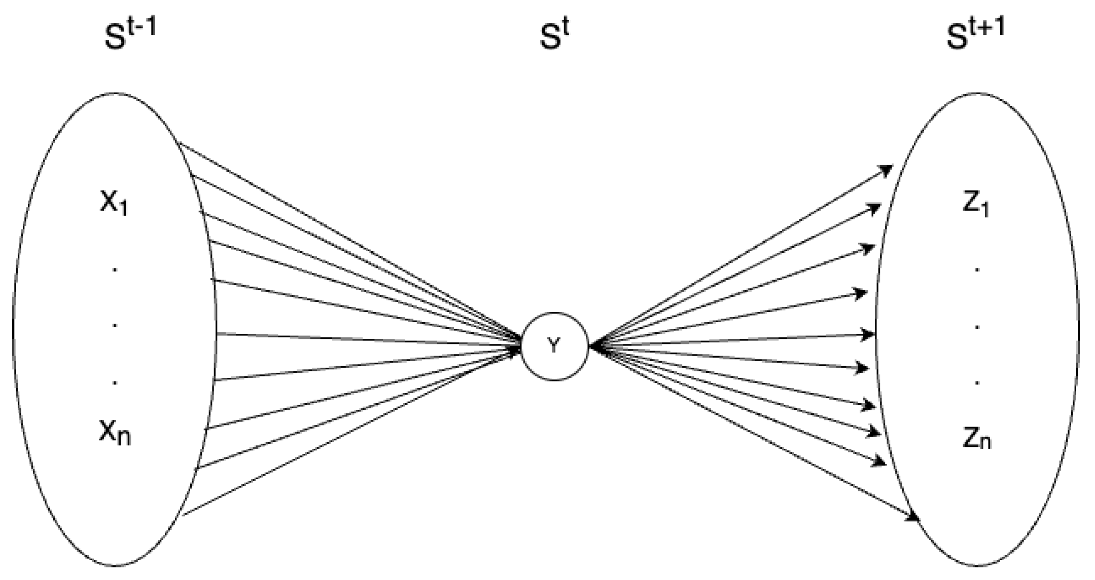
Figure 2.
Example of GoL grids evolution in time. Different initial states lead to different state transitions by the update of every cell on the grid at the same time. See text for further details. (Image taken from [81])
Figure 2.
Example of GoL grids evolution in time. Different initial states lead to different state transitions by the update of every cell on the grid at the same time. See text for further details. (Image taken from [81])
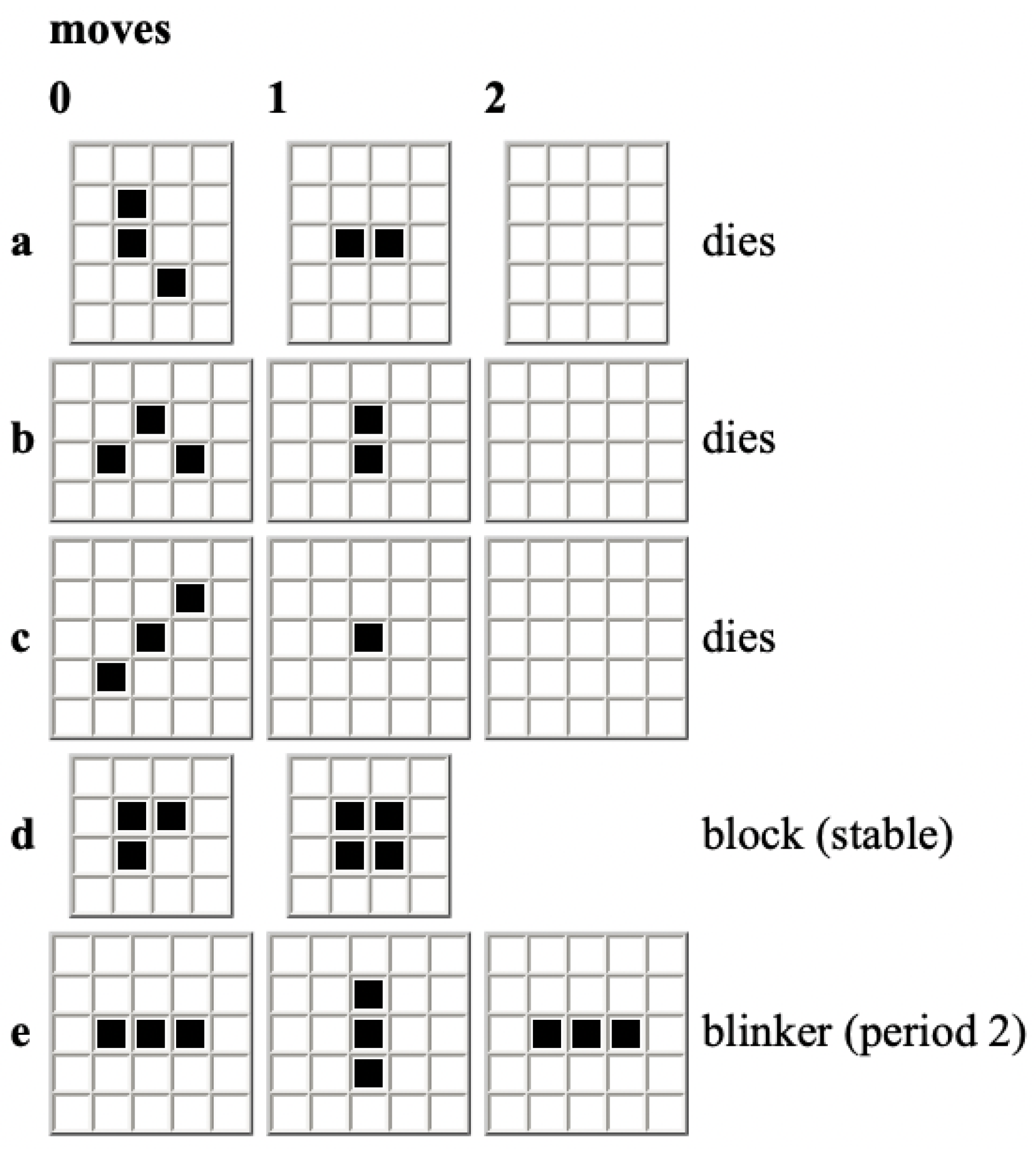
Figure 3.
Structural patterns in GoL that were investigated. Green represents active cells, black non-active cells acting as the `membrane’ of the system, whereas blue represent the environmental cells surrounding the system, which may be active or not.
Figure 3.
Structural patterns in GoL that were investigated. Green represents active cells, black non-active cells acting as the `membrane’ of the system, whereas blue represent the environmental cells surrounding the system, which may be active or not.
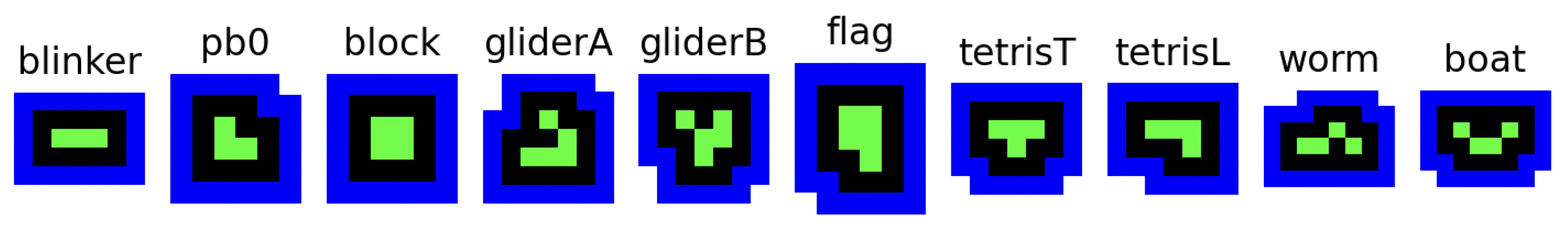

Table 1.
Table displaying the possible system-environment combinations and their resulting state transitions, for a single cell in the GoL.
Table 1.
Table displaying the possible system-environment combinations and their resulting state transitions, for a single cell in the GoL.
| Total | |||
| 28 | 0 | 28 | |
| 0 | 56 | 56 | |
| 172 | 0 | 172 | |
| 0 | 28 | 28 | |
| 0 | 56 | 56 | |
| 172 | 0 | 172 | |
| Total | 372 | 140 | 512 |
Table 2.
Table displaying only environmental states encountered before transitioning and their correspondent resulting states. Hence, as environment-to-system influence
Table 2.
Table displaying only environmental states encountered before transitioning and their correspondent resulting states. Hence, as environment-to-system influence
| Total | |||
| 2 | 28 | 28 | 56 |
| 3 | 0 | 112 | 112 |
| q | 344 | 0 | 344 |
| Total | 372 | 140 | 512 |
Table 3.
Entropy values obtained from the repertoires, measuring system-system influence. stands for , so for the entropy of such distributions.)
Table 3.
Entropy values obtained from the repertoires, measuring system-system influence. stands for , so for the entropy of such distributions.)
| blinker | pb0 | block | gliderA | gliderB | flag | tetrisT | tetrisL | worm | boat | entropy | |
| blinker | 0.091 | 0.337 | 0 | 0.073 | 0 | 0 | 0.018 | 0.085 | 0.178 | 0 | 1.969 |
| pb0 | 0 | 0.285 | 0.119 | 0 | 0.035 | 0.253 | 0.062 | 0 | 0 | 0 | 1.298 |
| block | 0 | 0.126 | 0.233 | 0 | 0 | 0.441 | 0 | 0 | 0 | 0 | 0.867 |
| gliderA | 0.285 | 0.282 | 0.022 | 0 | 0.020 | 0.020 | 0.090 | 0.071 | 0.017 | 0 | 1.948 |
| gliderB | 0.051 | 0.657 | 0.024 | 0 | 0 | 0 | 0.071 | 0.075 | 0.014 | 0.032 | 1.271 |
| flag | 0.182 | 0.185 | 0.045 | 0.001 | 0.001 | 0.164 | 0.071 | 0.165 | 0 | 0.015 | 1.914 |
| tetrisT | 0 | 0.612 | 0 | 0 | 0 | 0.248 | 0.140 | 0 | 0 | 0 | 0.830 |
| tetrisL | 0.120 | 0.429 | 0 | 0.005 | 0.003 | 0.014 | 0.096 | 0.019 | 0.032 | 0 | 1.544 |
| worm | 0.164 | 0.175 | 0 | 0 | 0.015 | 0.224 | 0 | 0 | 0.044 | 0 | 1.155 |
| boat | 0.324 | 0.288 | 0 | 0 | 0 | 0.102 | 0 | 0.036 | 0 | 0 | 1.217 |
Table 4.
Comparison of entropy values obtained from the repertoires correspondent to the GoL patterns from Figure 3. stands for the state of the system, while is short for , hence for the environment-system repertoires. The notation stands for `not found’. The subindices and refer to the next maximum entropy value for each (or the next after blinker and pb0, if lower) and minimum respectively (further details in the main text).
| blinker | 0.633 | 1.322 | tetrisL=0.381 | =0.030 |
| pb0 | 1.583 | block=0.389 | =0.089 | |
| block | 0.570 | flag=0.687 | block=0.133 | |
| gliderA | 0.235 | 1.251 | tetrisL=0.151 | =0.011 |
| gliderB | 0.767 | 1.340 | tetrisL=0.266 | =0.065 |
| flag | 0.644 | 0.949 | =0.352 | =0 |
| tetrisT | 2.060 | flag=0.591 | tetrisT=0.525 | |
| tetrisL | 1.352 | 1.853 | flag=1.139 | =0.120 |
| worm | 0.986 | 0.929 | worm=0.524 | =0.095 |
| boat | 1.445 | 1.314 | flag=0.740 | tetrisL=0.373 |
Disclaimer/Publisher’s Note: The statements, opinions and data contained in all publications are solely those of the individual author(s) and contributor(s) and not of MDPI and/or the editor(s). MDPI and/or the editor(s) disclaim responsibility for any injury to people or property resulting from any ideas, methods, instructions or products referred to in the content. |
© 2025 by the authors. Licensee MDPI, Basel, Switzerland. This article is an open access article distributed under the terms and conditions of the Creative Commons Attribution (CC BY) license (http://creativecommons.org/licenses/by/4.0/).
Copyright: This open access article is published under a Creative Commons CC BY 4.0 license, which permit the free download, distribution, and reuse, provided that the author and preprint are cited in any reuse.


