
Submitted:
29 September 2024
Posted:
30 September 2024
You are already at the latest version
Abstract
Wind power has emerged as a crucial substitute for conventional fossil fuels. The combination of advanced technologies such as the internet of things (IoT) and machine learning (ML) has given rise to a new generation of energy systems that are intelligent, reliable, and efficient. The wind en-ergy sector utilizes IoT devices to gather vital data, subsequently converting them into practical insights. The aforementioned information aids among others in the enhancement of wind turbine efficiency, precise anticipation of energy production, optimization of maintenance approaches, and detection of potential risks. In this context, the main goal of this work is to combine the IoT with ML in the wind energy sector by processing weather data acquired from sensors to forecast wind power generation. To this end, three different regression models are evaluated. The models under comparison include Linear Regression, Random Forest, and Lasso Regression, evaluated us-ing metrics such as coefficient of determination (R²), adjusted R², mean squared error (MSE), root mean squared error (RMSE), and mean absolute error (MAE). After examining a dataset from IoT devices that included weather data, the models provided substantial insights regarding their ca-pabilities and responses to preprocessing, as well as each model's reaction in terms of statistical performance deviation indicators. Ultimately, the preprocessing and the data analysis show that Random Forest regression is more suitable for weather condition datasets than the other two re-gression models. Both the advantages and shortcomings of the three regression models indicate that their integration with IoT devices will facilitate successful energy forecasting.
Keywords:
internet of things
; machine learning
; data analysis
; regression analysis
1. Introduction
Given the increasing environmental concerns and the need to shift to sustainable energy sources, wind power has emerged as a significant and feasible alternative to conventional fossil fuels [1]. Wind farms, comprised of a collection of wind turbines, have become essential structures in the worldwide effort to provide environmentally friendly and sustainable energy [2]. The increasing interest in wind energy coincides with a crucial phase in the energy sector, marked by the integration of advanced technologies like the IoT and ML. These state-of-the-art technologies are not simply enhancing the abilities of current energy systems; they are completely transforming them. They pledge to introduce a new era marked by intelligent, reliable, and extremely efficient energy systems that not only improve performance but also tackle urgent energy issues worldwide. The wind energy sector is progressively utilizing IoT devices to collect vital data, playing a key role in this technological transformation [3]. The features may encompass parameters like wind speed, wind direction, temperature, humidity, air pressure, and metrics related to the health of the turbine. These variables offer crucial insights into the elements that affect wind power output. Once gathered and examined, these data act as a catalyst for enhancing the effectiveness of wind turbines, precisely predicting energy generation, simplifying maintenance approaches, and identifying possible hazards. Furthermore, the instantaneous transfer of sensor measurements to distant control centers enables uninterrupted surveillance, although it presents certain difficulties, particularly with real-time control at the system and component levels. Currently, supervisory control and data acquisition (SCADA) systems offer advanced services and capabilities for wind energy conversion system (WECS) that go beyond basic monitoring and management of wind turbines, utilizing meteorological observations and weather data to forecast wind power generation [1].
This article provides foundational insights into IoT applications in wind energy systems, incorporating data analysis and ML through three different regression models. The preprocessing phase encompasses outlier removal, data transformation, correlation analysis, cross-validation, standardization and data splitting, all of which prepare the dataset for ML processing. To this end, an innovative approach is presented that involves preprocessing followed by Linear, Random Forest, and Lasso regression, yielding valuable results. The objective is to demonstrate how the utilization of these technologies can significantly enhance the efficiency, reliability, and ecological sustainability of wind energy systems, thereby facilitating the global transition towards a more sustainable and environmentally conscious energy sector.
In recent years, numerous scientific works have dealt with the deployment of IoT in wind energy and forecasting of energy output. The work in [3] examines the implementation of IoT in wind farms and the broader energy sector. It asserts that the incorporation of IoT into wind farms enhances the existing 743 GW worldwide wind power capacity to a sufficient level to provide 20% of the world’s electricity by 2030. In the same context, the obstacles related to the implementation of IoT in wind farms and the prospective role of blockchain technology and green IoT in energy systems are discussed as well. In [4], an IoT-based communication architecture is proposed to ensure reliable connection between wind turbines and the control center, utilizing repeat-accumulate coded communication to improve reliability. The numerical findings indicate that the suggested technique can accurately predict the condition of a wind turbine and greatly surpasses previous estimating methods. In [5], a set of multiobjective predictive models was developed employing various advanced ML algorithms, such as artificial neural networks (ANNs), recurrent neural networks (RNNs), convolutional neural networks (CNNs), and long short-term memory (LSTM) networks. According to the outcomes of this work, the LSTM, RNN, CNN, and ANN algorithms were effective in predicting wind power. The efficacy of these models was assessed by the integration of statistical metrics for performance deviation. In conclusion, the LSTM model is more effective in predicting wind power. In [6], long-term wind power forecasting was conducted utilizing daily wind speed data through five machine learning algorithms: LASSO regression, k-nearest neighbors (kNN) regression, xGBoost regression, random forest regression (RFR), and support vector regression (SVR).The findings of this work indicated that ML algorithms are capable of predicting long-term wind power values based on previous wind speed data and can be utilized in sites distinct from those used for model training. Among these algorithms, RFR had improved performance compared to the other approaches, while LASSO had the worst performance metrics due to its linear basis.
In all the aforementioned studies, the researchers concentrate their efforts either on IoT in wind energy or in wind power forecasting. Therefore, a key novel point of this work is the integration of IoT technology with wind energy systems and the comparison of fundamental ML algorithms to extract valuable information. To this end, this work initially examines the design and architecture of WESCS in wind energy, followed by an exploration of ML, particularly focusing on three regression models and their capabilities.
The rest of this paper is organized as follows: In Section 2, the incorporation of IoT in the wind energy sector is analyzed, and in particular the composition of WESC, the cyber-physical integration of a wind turbine, the SCADA systems, and machine to machine (M2M) for internet of everything (IoE)-enabled wind farms. Section 3 is focused on ML in wind energy forecasting. To this end, the data and preprocess steps are described, with an emphasis on regression analysis. In the same context, Linear, Random Forest, and Lasso models are then analyzed, with their basic characteristics and results on various key performance indicators (KPIs), including cross-validation results. In Section 4, KPIs’ performance is presented on the test set and cross-validation, concluding with the complexity and interpretability of the models. Finally, concluding remarks are outlined in Section 5.
2. IoT and Wind Energy
The efficacy and magnitude of wind technologies are advancing at a rapid pace. The energy specialists have ambitious goals for the future integration of wind energy into the industry. The primary challenge in the advancement of wind energy lies in the inherent unpredictability of these resources. Therefore, the real-time operation can make the necessary arrangements in the power system to counteract fluctuations without experiencing sudden changes in power output. Furthermore, the availability of real-time data sharing is essential for effective collaboration between energy storage facilities and wind units [7]. Figure 1 illustrates IoT’s contribution to the wind energy sector, using weather data as input and providing real-time, accurate information for energy forecasting.
Furthermore, the use of IoT technology in conjunction with information and communications technology (ICT) infrastructures enables wind farm operators to effectively implement precise predictive maintenance schedules, thereby mitigating the risk of incurring substantial losses. A timetable of this nature can be implemented through the utilization of ML and data mining methodologies. Timely maintenance can lower the levelized cost of energy (LCoE) index for wind assets [8]. The LCoE index quantifies the discounted value of the average cost of electricity over the whole operational lifecycle of the turbines. The indispensability of IoT in harnessing wind energy lies in the prompt collection and analysis of data pertaining to wind turbines and wind farms. Currently, the challenges of data transfer latency for offshore wind farms and the restricted capacity to transmit information to distant areas are two significant difficulties that need to be resolved. Hence, by gathering and examining crucial data in real-time, the process of making decisions, such as the prompt shutdown of a turbine to prevent further damages, can be expedited or even automated [4]. The integration of IoT technologies in the wind industry emphasizes the necessity for more holistic approaches to develop economical, secure, and reliable frameworks for the planning, operation, installation, and maintenance of wind farms and turbines.
Typically, wind farms are placed in distant areas, resulting in control centers being situated many hours away from the wind farms. Utilizing an IoT network, remote data transmission connectivity can enable control centers to effectively monitor the condition of a wind turbine and exert control over its operation [4]. Wind turbines, being located in remote areas, necessitate the use of wireless networks like cellular or satellite networks for IoT network access. Figure 2 illustrates a combined system consisting of wind turbines and a wireless IoT network.
2.1. Composition of WECS
Physical Layer in WECS: The wind energy conversion system comprises the following physical components: blades, rotor hub, nacelle, and tower foundations, as shown in Figure 3. The nacelle consists of several components, including shafts, gearbox, generator, and other electrical and mechanical systems. The various components are continuously monitored and regulated by a multitude of sensors and actuators [9]. The wind turbine is fitted with sensors that quantify multiple characteristics related to the functioning and state of each component. Simultaneously, the control system governs and manages the functioning of the wind turbine through a sequence of actuators.
Cyber Layer in WECS: The cyber layer in WECS incorporates a variety of hardware and software technologies that collaborate to accomplish shared goals [9]. The cyber layer typically comprises networking, SCADA, and content management systems (CMS) as illustrated in Figure 4.
Networking: Reliable communication networks between subsystems within a wind turbine are necessary for the successful deployment of WECS. Furthermore, it facilitates the connection of sophisticated machinery and intricately integrated devices across a wind farm. Networking essentially enables the efficient transmission of data and control signals among con-trollers, actuators, sensors, supervisory centers, and data storage stations [10]. When developing communication networks for wind farms, especially those located offshore, it is crucial to take into account many factors such as data transmission rates and network resilience.
Various sensors are integrated inside a wind turbine to measure its numerous components, such as the generated current, voltage, and rotor speed. Let be the measured state by the sensor of the wind turbine. We define by,
- : A vector of measurements with dimension , where is the number of components or parameters being measured by the sensor.
- : A matrix that represents the measurement or sensing data from sensor with dimensions where is the number of measurements or components observed by the sensor and n refers to the number of state variables of the system being observed by the sensors.
- : A vector contains the state variables that describe the system’s internal dynamics, such as electrical power generation, rotor speed, or internal parameters that are being monitored or controlled.
The matrix represents the measurement or sensing data from sensor , while represents the observed noise during the measurement at sensor . The measurement noise is modeled as Gaussian noise with zero-mean and covariance , similar to the process noise. The measured state is transmitted at regular intervals to the control center for the implementation of the necessary actions. As wind turbines are generally located in remote areas, there is frequently no direct communication link between a wind turbine and the control center. Normally, the transmitter of a wind turbine establishes a connection with a nearby base station, which subsequently transmits the message to the control center. The communication link between the base station and control center is assumed to be reliable, as it is part of a solid backbone network. However, the wireless communication link between the wind turbine and the base station encounters challenges in ensuring reliable data transmission [4]. Dependable communication is crucial for precise state estimates and control applications. The observed state is denoted as , where represents the measurement of the component of X obtained from the sensor. Every element of is transformed and discretized into K bits. The bit block that corresponds to the component is represented by , where . Next, a repeat-accumulate code is used on to produce a code word, where c refers to the encoded bits or codewords. The codewords are organized in a sequential manner to create . Once the is modulated onto the wireless carrier signal, the resulting carrier signal is transmitted from the wind turbine to the base station:
where represents the additive white gaussian noise (AWGN) with a mean of zero and a standard deviation of and is the fading component. After receiving , the receiver carries out the inverse procedure (such as demodulation, decoding, demapping, etc.) to create the observed state. Figure 5 depicts the communication architecture for wind turbines based on IoT sensors.
SCADA and CMS: Currently, SCADA systems offer advanced services and capabilities for WECS that go beyond basic monitoring and management of wind turbines. CMSs are essential systems that are seamlessly connected with SCADA systems. CMSs utilize a variety of methods to detect defects in wind turbines at an early stage. The incorporation of CMS has shown significant improvements in the functioning and upkeep of wind turbines. CMS systems commonly employ a greater number of sensors with higher sample frequencies, as opposed to SCADA systems [9]. CMSs provide significant advantages in data communication, calculation, and storage, in addition to increasing overall costs. Consequently, numerous proposals are put forward to utilize SCADA data for condition monitoring in order to decrease the expenses of wind energy conversion systems [11]. Nevertheless, a thorough examination of specialized CMS in comparison to SCADA-based configuration management (CM) reveals that CMS are considerably more expensive but possess more diagnostic capabilities due to their higher frequency of information.
2.2. Cyber Physical Integration of a Wind Turbine
Upon conducting a thorough analysis of the many components of WECS, it is evident that they can be classified as intricate technologies that incorporate embedded systems. The cooperation between WECS layers, as depicted in Figure 6 exhibits a significant degree of diversity and constitutes a characteristic cyber-physical system (CPS) [9]. Viewing WECS as CPS introduces additional levels of technology adaption and amplifies the capabilities of WECS to be seamlessly included into intelligent power grids and the IoE.
The advancement of CPS necessitates the creation of novel models and design approaches. The primary objective of these new models and methodologies is to strike a harmonious equilibrium between intricacy and practicality. Integrating all diverse components of the cyber and physical levels to model wind turbine systems poses a significant challenge. Various elements of characteristics must be taken into account when creating CPS compositional models, including functional, non-functional, physical, component interfaces, and interface coordination. Thus, the intricate and diverse nature of components in contemporary wind turbines necessitates the application of similar concerns to be extended to WECS. It is necessary to use comprehensive analysis and verification methods to guarantee the precise operation of control systems for different electrical and mechanical components. Moreover, it is important to furnish comprehensive models of wind resources and electrical loads that influence the operational conditions. In the same context, it is imperative to establish a framework to guarantee the continuous viability, protection, defense, and adaptability of WECS [11].
Verification techniques are necessary to assess the physical requirements, such as size, power, dynamics, and memory, of various computing and networking components used in wind turbines within the context of CPS. Additionally, there is a requirement for tools to verify the compatibility of various interfaces of SCADA, CMS, sensor nodes, and power electronics with control circuits [4]. Future WECS necessitate the implementation of unified techniques to enhance their extensibility, facilitate interaction with smart grids, and improve human-machine interfaces [7]. WECS models are expected to incorporate both continuous physical dynamics and discrete occurrences. There needs to be a consistent understanding of time across sensor nodes, network, and computing platforms. In addition, contemporary wind turbine technology incorporates computing systems that operate at varying speeds [12]. SCADA systems in wind facilities function at a low frequency to record performance data, whereas CMS operate at a high frequency to monitor components effectively. Moreover, it is imperative to depict the tangible movements of mechanical structures, the study of airflow around objects, the behavior of electrical parts, and the control of electrical power using descriptive programming abstractions. Therefore, it is becoming more and more necessary to combine conceptual computational and information flow models from sensor networks with physical mechanical and electrical models in wind turbines. Alternatively, black box approaches can be used, relying on system identification using real data obtained from wind facilities.
2.3. SCADA Systems and M2M for IoE-Enabled Wind Farms
Due to the harsh, expansive, and isolated nature of wind farm sites, SCADA systems must possess the ability to efficiently monitor and control operations. Furthermore, the intricate nature of a wind turbine necessitates the perception of wind farms as a collection of interconnected systems. Hence, it is imperative to enhance the existing SCADA systems employed for monitoring and controlling grids and power plants, including wind turbines, by including advanced multilayered interactive sensing, communication, and control functionalities. It is imperative to fulfill the requirements of upcoming industrial and energy needs [12]. Presently, energy providers are requiring the incorporation of wind farms SCADA systems into their asset management software, such as enterprise resource planning (ERP) and customer resource management (CRM). Figure 7 presents a concise overview of the responsibilities and objectives that upcoming SCADA systems for wind energy will encompass.
In the future, wind farms will require the use of CP SCADA systems that are implemented using IoT technology for their operation and management. The notion of the IoT is exemplified by the implementation of a wireless sensor network (WSN) for an industrial process, which allows for remote monitoring via the internet [11,13]. A customizable SCADA system with decentralized intelligence and decision-making capabilities is provided based on a CP model of a power system. The system comprises three primary elements: Intelligent machines, analytics, and operators. This concept is employed in a wind control platform to oversee the synchronization of wind turbines in a farm. The SCADA system is anticipated to leverage current advancements in computing and networking to offer monitoring and control services via the internet, aligning with the fundamental essence of the IoT. Efficiently processing large amounts of raw data requires the use of self-organizing CPS networks. Hence, CP wind farms necessitate the implementation of novel network standards, protocols, and infrastructures. M2M communications is an increasingly important component of the IoT [14]. M2M connections enable the transmission of information between intelligent equipment, business applications, and data servers. Anticipated developments in M2M technology will broaden the scope of connections beyond individualized interactions to a model where producers and consumers are interconnected. A planned infrastructure for M2M communications aims to enable smart wind farms to efficiently communicate measured data and enhance their intelligence among wind turbines. A proposed cloud based M2M telemetry system aims to efficiently handle and visually represent data for suppliers of renewable energy [15]. Furthermore, content management systems are getting more intelligent using M2M technology.
3. ML for Wind Energy Forecasting
This section delineates the procedures for data collecting, data pre-processing, and the implementation of machine learning algorithms.
Wind energy forecasting analysis jobs involve the processing and interpretation of large quantities of weather-related data to generate accurate estimates of future energy generation. These tasks employ a diverse range of analytical methodologies and tactics to enhance the precision of forecasts. The meteorological data, consisting of wind speed, wind direction, temperature, humidity, wind gusts, and dewpoint, is now accessible and can be utilized for power generation predictions, as Figure 8 shows [15]. Significant statistical connections can be identified between different meteorological factors and energy production. These correlations can be used to construct models that accurately represent the influence of certain weather conditions on the efficiency of wind turbines. The selection of features for forecasting models is determined by this examination. Selecting suitable machine learning techniques, like regression models, for predictive modeling depends on the unique demands of the forecasting issue and the features of the data.
3.1. Dataset and Preprocessing
The Wind Power Generation Data - Forecasting dataset was acquired from Kaggle (https://www.kaggle.com/datasets/mubashirrahim/wind-power-generation-data-forecasting/data) and uploaded to the Kaggle platform by MUBASHIR RAHIM. The meteorological equipment – IoT devices deployed at the site was used to meticulously gather the data. The meteorological apparatus measured temperature, humidity, dew point, and wind properties at predetermined elevations of 2 meters, 10 meters, and 100 meters. Concurrently, sensors were installed on wind turbines to monitor their efficiency and electricity production. The datasets consist of a detailed hourly log obtained from four distinct sites, spanning from January 2, 2017, 00:00:00, to December 31, 2021, 23:00:00. The data underwent rigorous quality checks to detect and rectify any anomalies or inconsistencies, ensuring a high level of data reliability. Regular equipment maintenance has consistently ensured the quality of data over time.
The following are the columns and weather parameters in the data:
- Time: The moment in the day when the measurements were made.
- temperature_2m: The temperature in degrees Fahrenheit at two meters above the surface.
- relativehumidity_2m: The proportion of relative humidity at two meters above the surface.
- dewpoint_2m: Dew point, measured in degrees Fahrenheit at two meters above the surface.
- windspeed_10m: The wind speed, expressed in meters per second, at 10 meters above the surface.
- windspeed_100m: The speed of the wind at 100 meters above sea level, expressed in meters per second.
- winddirection_10m: The wind direction at 10 meters above the surface is represented in degrees. (0-360).
- winddirection_100m: The direction of the wind at 100 meters above the surface, expressed in degrees (0–360).
- windgusts_10m: A wind gust is an abrupt, transient increase in wind speed at 10 meters.
- Power: The normalized turbine output, expressed as a percentage of the turbine’s maximum potential output, and set between 0 and 1.
The normal or Gaussian distribution that is indicated in Figure 9 represents the famous bell-shaped curve, which is characterized by the arithmetic mean μ and the standard deviation σ. The normal distribution is the most frequently employed probability and statistics distribution. Contemporary techniques like as linear regression, analysis of variance (ANOVA), and t-tests heavily depend on the assumption that the data follows a normal distribution. Because the dataset contains outliers, which indicate the accuracy of the sensors’ measurements, the curves do not have a well-defined shape [16].
Libraries: Python’s libraries for data analysis, visualization, and scientific computing are extensively utilized. They provide a comprehensive range of tools and features that make it easier to explore data and generate insights [17]. The libraries to be utilized in the preprocessing stage are as follows:
- Pandas is a robust Python package utilized for the manipulation and analysis of data. The software provides data structures such as DataFrames and Series, which facilitate the manipulation and analysis of organized data.
- NumPy is an essential library for scientific computation in Python, commonly referred to as “Numerical Python.” The software provides support for large, complex arrays and matrices, together with a collection of mathematical algorithms to effectively handle these arrays.
- Matplotlib is a flexible toolbox that enables the generation of static, interactive, and animated visualizations in the Python computer language. The pyplot module offers a MATLAB-like interface for producing plots and visualizations, simplifying the process of generating charts, histograms, scatter plots, and other graphical representations.
- Seaborn is a data visualization package that enhances the capabilities of matplotlib and provides a more sophisticated interface for creating visually appealing and meaningful statistical graphics. It streamlines the procedure of generating intricate visualizations and provides pre-installed themes and color palettes to increase the visual appeal of plots.
Dataset: There are four data frames, namely loc1, loc2, loc3, and loc4, that are all of equal size. All data in the datasets originates from the utilization of IoT devices to measure meteorological conditions with consistent precision. The number of rows in each data frame is 43800, and the number of columns is 10. This study centers on the examination carried out utilizing the loc1 dataset. The columns consist of the following variables: time, temperature, relative humidity, dewpoint, wind direction, wind speed, and wind gusts at 2, 10, and 100 meters, as shown in the first 5 rows of Figure 10. There are six variables of float64 data type, three variables of int64 data type, and one variable of object data type.
Since time is an object, it will be transformed to datetime before being used for analysis. The conversion is performed using the function (pd.to_datetime) from the Pandas package [17]. The subsequent tables and figures originate from the exploratory data analysis conducted at loc1. Based on the corresponding time values, in Table 1, organize the power-generating data into separate columns for year, month, and day.
Null values: A non-null value refers to any numerical, textual, or other type of value that is not null [18]. The data frame has 43,800 non-null values in each column, corresponding to the index range of 0-43799. By utilizing Python’s function .null().sum(), can determine the number of null values for each variable. Datasets do not contain any null values as described in Table 2. Determining influential and anomalous data points is essential as it will aid in future data collection and the proper utilization of existing knowledge.
Outliers: The degree to which a data point deviates from the mean in terms of standard deviations is measured statistically by the z-score [18]. The z-score can be calculated using the following formula:
In this context, x represents a specific data point, mean represents the average value of the dataset, and std represents the standard deviation of the dataset.
It appears that the dataset contains some outliers, as illustrated in Figure 11 Consequently, Table 3 shows the results of removing outliers to achieve improved outcomes.
The distribution of wind gusts in Figure 12 may show significant skewness due to extreme values, which can obscure the true underlying patterns. After outlier removal, the distribution typically becomes more normal, allowing for clearer insights and more accurate analyses.
Correlation: The dataset is currently accessible and prepared for utilization in deriving significant insights. Correlation study between measurements such as temperature, relative humidity, and wind speed will assist in selecting parameters for prediction [19]. These highly correlated metrics aid in forecasting the power generated by wind turbines. A correlation heatmap is a visual representation that presents the correlation between many variables in the form of a matrix, utilizing color codes. By utilizing the Python programming language and the seaborn library, it is possible to generate a helpful heatmap that displays the association between variables. The correlation coefficients for various variables are displayed in a correlation table.
Conventional clustering and correlation analysis face difficulties when dealing with the vast amount and low density of valuable information in big data. To improve energy forecasting, it is recommended to use big data-driven correlation analysis with clustering. Conducting correlation analysis among several measures such as temperature, dew point, relative humidity, wind direction, wind gusts, and wind speed will aid in the selection of forecast parameters. These strongly connected parameters contribute to the accurate prediction of the electricity produced by wind turbines.
The heatmap in Figure 13 displays the relationships between every conceivable combination of values. It is a potent tool for detecting and visualizing patterns in data, as well as condensing large amounts of data. A Python program, utilizing the Seaborn module, may generate a heatmap that visually represents the association between variables [16].
When preparing a dataset for ML models, preprocessing stages include data standardization and splitting. Consequently, all three regression models (linear regression, random forest regression, and lasso regression) follow this preprocessing phase.
Standardization: This procedure guarantees that the dataset’s features (or variables) have a mean of 0 and a standard deviation of 1 [20,21]. This phase is essential as numerous ML algorithms exhibit enhanced performance when the data is normalized or standardized. The StandardScaler is a prevalent technique that subtracts the mean and normalizes data to unit variance.
The standardization formula for each feature x is as follows:
- is the mean of the feature.
- is the standard deviation of the feature.
Splitting the data: This pertains to partitioning the dataset into training and testing (and occasionally validation) subsets [21]. The training set is utilized to develop the model, whereas the testing set is employed to assess its performance on novel data. The validation set is also employed to optimize the model without affecting the test set, particularly during hyperparameter optimization. This mitigates overfitting and guarantees the model generalizes effectively to novel inputs. The data is typically divided between 70% and 80% for training and 20% and 30% for assessment. The precise ratio is contingent upon the task at hand and the extent of the dataset. After completing the data purification procedure, the dataset (loc1) is now available and ready to be used for extracting meaningful insights.
3.2. Machine Learning and Wind Energy Forecast
ML algorithms have the capability to identify alterations in the surroundings and adjust their actions accordingly. Regression analysis refers to this specific subset of categorization [22,23]. The objective of this part is to structure the forecasting in the wind energy domain. Following the technique or data analysis, ML is employed to predict the power energy output. This extensive dataset provides valuable insights on the correlations between various weather patterns and the generation of wind energy. By using predictive models and analyzing meteorological data, it’s feasible to forecast power output.
Regression models are utilized to determine the correlation between alterations in one or more explanatory variables and alterations in the dependent variable. To determine the regression model that exhibits the greatest efficiency and the lowest mean square error (MSE), three regression models will be used and compared [24]. The comparison of linear regression, random forest regression, and lasso regression will yield valuable results and provide an opportunity to gain a more comprehensive comprehension of each regression model and the capabilities of each other.
Regression is extensively used in the field of big data to build predictive models. These models are designed to forecast certain outcomes for incoming data, rather than interpreting existing data. Regression analysis is a reliable method for identifying the variables that have an impact on a specific topic of interest [23]. Regression analysis allows for the accurate identification of the key aspects, the ones that may be ignored, and the correlations between these elements.
- Dependent Variable: The dependent variable is the primary factor that one seeks to anticipate or comprehend.
- Independent Variables: These variables are postulated to exert an influence on the dependent variable.
- The metrics included in the regression models are R2, Adjusted R2, MSE, RMSE, and MAE.
- R2 (Coefficient of Determination): Assesses the model’s efficacy in elucidating the variance of the target variable. Varies from 0 to 1, with proximity to 1 indicating a superior fit [24].
- Adjusted R2: Analogous to R2, although modified to account for the quantity of predictors in the model. Addresses overfitting; increases solely if additional predictors enhance the model.
- MSE: The mean of the squared deviations between expected and actual values. Imposes more penalties on larger faults compared to lesser ones.
- RMSE: The square root of the MSE. Denotes the mean error in the identical units as the target variable.
- MAE: The mean of the absolute discrepancies between expected and actual values. More robust to outliers than MSE or RMSE.
Overfitting in ML occurs when models are selected and hyperparameters are adjusted based on test loss, which challenges the assumption that the model’s performance is independent of the test set [25]. The ultimate classifier may exhibit high performance only on a certain sample of examples within the test set, especially when method designers evaluate numerous models on the identical test set [26]. K-fold cross-validation is used to assess the performance of predictive models. The dataset is partitioned into k folds, each of which is a subset. As shown in Figure 14, for each of the k training and assessment cycles, the model uses a distinct fold as the validation set. The model’s generalization performance is measured by calculating the average of the performance metrics obtained from each fold.
3.2.1. Linear Regression
Linear regression, sometimes known as LR, is a prevalent and extensively utilized modeling technique in the fields of statistics and machine learning. The objective outcome is to establish a linear relationship between the input and target variables. The model postulates a linear amalgamation of the input features to predict the continuous output variable. In order to calculate the coefficients of these input variables, several optimization approaches, such as least squares, are utilized [27]. LR is an excellent option when there are linear relationships between variables due to its simplicity and ease of comprehension. Multiple linear regression (MLR) is an appropriate form of linear regression for this particular situation. MLR produces equations that establish a connection between several input variables () and a target variable ().
Here, n represents the total number of input variables, denotes the coefficient for , and refers to the intercept. Regularization approaches, such as the inclusion of a penalty term on the model’s input variables, can restrict the freedom of the input variables during the learning process, hence improving the accuracy of predictions on data that was not used for training.
MLR is a statistical technique that estimates the value of a dependent variable based on multiple independent variables. The objective of MLR is to construct a precise mathematical model that accurately depicts the linear relationship between the independent variables () and the dependent variable () being studied [28]. The primary MLR model is described as:
- is the dependent variable.
- is the intercept.
- The coefficients represent the values assigned to the independent variables .
The intercept, often known as the “constant,” in a regression model signifies the average value of the response variable when all predictor variables in the model are set to zero. The intercept, denoted as , is the estimated value of y when all xi values are equal to zero. The baseline level of (dependent variable) is established when the explanatory variables have no influence. The coefficients represent the weights of each independent variable, indicating the extent to which each variable contributed to the prediction.
The implementation of the linear regression technique, along with cross-validation results, yielded the aforementioned metrics [24]:
- R2 (0.6199): This means that about 61.99% of the variance in the target variable can be explained by the model’s features. This indicates a moderately strong fit, but there is still 38% of variability in the target that the model does not explain.
- Adjusted R2 (0.6194): The Adjusted R2 is slightly lower than the R2 (0.6194 vs. 0.6199), which accounts for the number of predictors. It’s close to R2, suggesting that the added features are useful, but not overfitting.
- MSE (0.0312): The low value of 0.0312 of MSE indicates that the model’s predictions are generally close to the actual values, though it’s harder to interpret MSE without comparing it to the scale of the data.
- RMSE (0.1767): An RMSE of 0.1767 means that, on average, the model’s predictions are off by around 0.18 units from the actual values.
- MAE (0.1389): An MAE of 0.1389 means that, on average, the model is off by 0.14 units, which is slightly lower than the RMSE. This suggests the model is performing well with relatively small errors.
Cross-Validation Results (Mean ± Std): These results give insight into how the model performs across multiple data splits during cross-validation. They help confirm the robustness of the model.
- R2 (0.6299 ± 0.0082): The average R2 across cross-validation is 62.99%, slightly higher than the original R2. The standard deviation (±0.0082) indicates stable performance across different data splits.
- Adjusted R2 (0.6290 ± 0.0082): The adjusted R2 is 62.90% with minimal variability, confirming that the model generalizes well without overfitting.
- MSE (0.0303 ± 0.0007): The average error across cross-validation sets is 0.0303 with a small standard deviation (±0.0007), showing that the model is consistent.
- RMSE (0.1741 ± 0.0021): The average RMSE is 0.1741, meaning the average prediction error is about 0.174 units, with slight variability (±0.0021).
- MAE (0.1376 ± 0.0015): The average MAE is 0.1376, indicating that, on average, the model is 0.1376 units off. The small standard deviation (±0.0015) shows good consistency.
The cross-validation results validate the model’s stability, as the metrics consistently align across several data splits. Figure 15 displays the actual and predicted values, with residuals representing the differences between the actual and predicted values in a model.
3.2.2. Random Forest Regression
Leo Breiman [29] and Cutler Adele [30] proposed the Random Forest Regression (RFR) algorithm in 2001 as an ML method for both regression and classification tasks. Categorical regression tree (CART) techniques can be classified into two categories depending on the nature of the output variables: regression decision trees and categorical decision trees. It is a flexible ML technique employed for forecasting numerical values. In order to reduce overfitting and improve accuracy, it uses the predictions of many decision trees [31]. Python’s machine-learning modules facilitate the efficient optimization and implementation of this method.
Random forest regression involves adjustable parameters, similar to other ML techniques. Some of the factors that influence a regression tree include the minimum number of observations at each terminal node, the fraction of data to sample in each regression tree, the number of trees, and the number of predictor variables randomly picked at each node [32]. Cross-validation is employed to optimize these independent parameters. It is often recommended to set the number of decision trees to a high value in order to achieve a steady minimum for the prediction error, rather than making adjustments.
The equation for the generalization error and margin function in random forest is given as follows:
Where
The equation’s relevant term, , specifies the weighting of each tree’s vote to determine the final classification or regression output.
Let and represent random vectors. The margin function, mg, determines the average votes for the correct output compared to other outputs. The function I(.) is an indicator function, and represents the classifiers.
In Random Forest regression, RandomizedSearchCV is employed to optimize the model’s hyperparameters by exploring a spectrum of potential parameter values [33]. The get_param_grid method produces a dictionary of hyperparameters and their associated values for tuning in the Random Forest model. Each key in the dictionary signifies a hyperparameter (n_estimators: the number of trees in the forest, max_depth: the maximum depth of every tree in the forest, min_samples_split: the minimum number of samples required to split an internal node, min_samples_leaf: the minimum number of samples required to be at a leaf node) and the corresponding list comprises various values that RandomizedSearchCV will investigate.
The implementation of the RFR technique, along with cross-validation results, yielded the aforementioned metrics [34]:
- R2 (0.76087): An R2 of 0.76087 signifies that the model accounts for approximately 76.09% of the variance in the target variable, which is commendable. The model effectively catches most patterns within the data.
- Adjusted R2 (0.76060): Adjusted R2 is closely aligned with the R2, indicating that the model is appropriately fitted without superfluous complexity.
- MSE (0.01976): The MSE is notably low, signifying that the model’s prediction errors are minimal.
- RMSE (0.14057): An RMSE of 0.14057 implies that, on average, the model’s predictions diverge from the actual values by approximately 0.14 units, reflecting commendable performance, particularly relative to the data’s scale.
- MAE (0.10439): An MAE of 0.10439 indicates that, on average, the model’s predictions deviate by around 0.10 units. Given that MAE exhibits less sensitivity to outliers compared to MSE, it indicates that the model is continuously producing relatively minor mistakes.
Mean Cross-Validation Results: Better knowledge of how the model spans several subsets of the data comes from cross-valuation results. Often used against the single assessment on the test set, the “Mean” values show the average across several folds (splits) of the dataset.
- Mean Cross-Validation R2 (0.64517): With an average R2 value of 0.64517—lower than the test set R2—0.76087—over the cross-valuation folds. This implies that, on average, during cross-valuation, the model explains roughly 64.5% of the variation, whereas on the test set it explains about 76% of the variance. Although this difference suggests some variation in model performance over several data subsets, overall, the finding is still really strong.
- Mean Cross-Validation Adjusted R2 (0.64509): Considered as lower than the Adjusted R2 on the test set (0.76060), the average Adjusted R2 across cross-valuation is 0.64509. Like the R2 score, this indicates that although the model may be slightly overfitting the test data relative to its performance on several validation sets, it generalizes somewhat reasonably.
- Mean Cross-Validation MSE (0.02943): Higher than the test set MSE (0.01976), the average MSE among several cross-valuation folds is 0.02943. This implies that, on the test data, the model did rather better than on the average validation folds. Still, the variation is not significant, suggesting a rather steady performance.
- Mean Cross-Validation RMSE (0.17155): Higher than the test RMSE (0.14057), the average RMSE for the validation sets is 0.17155. This suggests that, although still within a reasonable range, the model’s mistakes during cross-valuation are rather greater than on the test set on average.
- Mean Cross-Validation MAE (0.13200): Higher than the test MAE, 0.10439, the average MAE during cross-valuation is 0.13200. Consequently, the model performs really well over several data splits but makes somewhat more mistakes on the cross-valuation folds.
Cross-validation results reveal that, when tested on several subsets of the data, the model’s performance is consistent but rather less. Although the lower cross-valuation R2 (0.64517) points to some variation in the generalizing capacity of the model, the test and cross-valuation metrics differ only in minor degree.
Currently, the evaluation of the model utilizing the most associated features, namely ‘windspeed_10m’, ‘windspeed_100m’, and ‘windgusts_10m’, yields the following results:
- R2 Score: 0.67234
- Adjusted R2 Score: 0.67223
- MSE: 0.02707
- RMSE: 0.16453
- MAE: 0.12603
By picking solely the most correlated features, the model may forfeit significant interactions or information offered by less correlated variables. The optimal parameters chosen yielded a less intricate model (fewer trees, reduced depth), which may not adequately depict the previous degree of intricacy. A strong correlation may not necessarily reflect a feature’s complete impact on a model’s performance, particularly in non-linear models such as Random Forests.
3.2.3. Lasso Regression
LASSO regression, also known as Least Absolute Shrinkage and Selection Operator regression, is a commonly employed method for reducing the size of coefficients and choosing variables in regression models. The computationally demanding nature of statistical software is no longer concerning due to developments in processing power and integration. The objective of LASSO regression is to identify the variables and corresponding regression coefficients that minimize the prediction error of the model [35]. A constraint is imposed on the model parameters to ensure that the total of the absolute values of the regression coefficients is smaller than a predetermined value (λ), hence causing the regression coefficients to be “shrunk” towards zero.
LASSO conducts regression analysis using the below equation, where represents the sample size of and , j denotes the parameter coefficients, represents the prediction.
The provided formula can be compacted and represented in Lagrangian form, as illustrated in the equation [36]. The equation below demonstrates that L1 regularization is the preferred method in LASSO. L1 regularization incorporates the absolute value of feature coefficients as a penalty term to regulate the impact of the features.
The implementation of the Lasso regression, along with cross-validation results, yielded the aforementioned metrics [37]:
- R2 (0.6110): This means that 61.10% of the variance in the target variable (y) is explained by the Lasso regression model. It’s a moderate grade, demonstrating that the model captures a good percentage of the variability, however there is potential for improvement.
- Adjusted R2 (0.6108): The Adjusted R2 value is quite close to the R2 score (0.6108 vs. 0.6110). This shows that the model’s performance does not diminish when accounting for the amount of predictors used. Since the model isn’t overfitting with irrelevant variables, the adjusted R2 stays virtually the same as the regular R2.
- MSE (0.0319): A lower MSE (0.0319) shows the model’s predictions are pretty close to the actual values, while there are some inaccuracies.
- RMSE (0.1787): RMSE is 0.1787, suggesting on average, the predictions are wrong by around 0.1787 units of the target variable, which is a substantial amount of inaccuracy.
- MAE (0.1410): With a MAE of 0.1410, the predictions average from the actual values by roughly 0.1410 units. This implies somewhat minimal error, although RMSE (which penalizes more significant errors) indicates somewhat more fluctuation in the errors.
Cross-Validation Results for Lasso Regression:
- Mean R2 (0.6132 ± 0.0533): With an average R2 score of 0.6132—rather close to the test set R2 of 0.6110—the 10 cross-valuation folds Although the performance of the model fluctuates somewhat throughout the few cross-valuation folds, the standard deviation (±0.0533) indicates minimal fluctuation that suggests consistency.
- Adjusted R2 (0.6108 ± 0.0533): With a mean of 0.6108, the modified R2 is also rather consistent; it indicates that the model can generalize effectively over several folds and is not overfitting.
- Mean MSE (0.0313 ± 0.0052): With a tiny standard deviation (±0.0052), the average MSE over the cross-valuation folds is 0.0313, somewhat near to the test set MSE of 0.0319. This indicates that the model is not unduly sensitive to several subsets of the data and is rather steady in performance.
- Mean RMSE (0.1769 ± 0.0722): Again, revealing a comparable average prediction error, the RMSE from cross-validation (0.1769) is once more near to the test set RMSE of 0.1787. Though it’s still reasonable, the standard deviation (±0.0722) indicates far more fluctuation in mistakes between folds than in MSE.
- Mean MAE (0.1399 ± 0.0105): With cross-validation, the average MAE (0.1399) is rather close to the test set MAE (0.1410). Furthermore, showing consistency in the prediction accuracy across several subsets is the low standard deviation (±0.0105).
The cross-validation outcomes closely align with the test set findings, indicating that the model generalizes effectively and is not overfitting the data. The minimal standard deviations for all measures indicate the model’s stability across various data splits.
4. Results and Discussion
This comparison analysis assesses the efficacy of three regression models: Linear Regression, Lasso Regression and RFR, utilized for wind power forecasting data. The performance of each model is evaluated using standard statistical metrics, such as R2, Adjusted R2, MSE, RMSE, and MAE. Furthermore, cross-validation was conducted to assess the models’ stability and generalizability. The following is a comprehensive comparison of the three regression techniques based on the data acquired. Initially, the Random Forest Regression and Linear Regression attain exceptionally high R2 and Adjusted R2 values, ranging from 0.98 to 0.99. Subsequent to preprocessing, it was observed that ML algorithms exhibit overfitting issues. In conclusion, preprocessing reduces the risk of overfitting, ensuring accurate predictions on both training and new data. The final results are presented in Table 4.
4.1. Performance Metrics on Test Set
- R2 and Adjusted R2: Random Forest exhibits enhanced predictive capability, evidenced by significantly elevated R2 and Adjusted R2 values relative to Linear and Lasso models. Both Linear and Lasso regressions exhibit comparable performance; however, Lasso slightly underperforms Linear Regression due to the effects of regularization. On Figure 16, the blue bar represents the RFR, the orange bar represents the LASSO regression, and the green bar represents Linear regression.
- MSE, RMSE, and MAE: The Random Forest model exhibits significantly lower MSE, RMSE, and MAE, underscoring its enhanced accuracy and diminished prediction errors. Linear Regression and Lasso have similar performance, while Lasso demonstrates somewhat inferior outcomes due to its penalization of certain characteristics. The differences are minimal, as evidenced by the proximity of each bar’s heights in Figure 17, but they have a significant impact.
4.1. Cross-Validation Results
- R2 and Adjusted R2: The Random Forest algorithm has improved performance on average over cross-validation folds, however it displays significantly greater variability than on the test set. Linear Regression exhibits marginally superior performance compared to Lasso in cross-validation, although the disparity is negligible.
- MSE, RMSE, and MAE: Random Forest consistently surpasses both linear and Lasso regressions in terms of MSE, RMSE, and MAE throughout cross-validation folds, exhibiting a narrower error range. Linear Regression exhibits marginally superior cross-validation performance compared to Lasso; yet, both models demonstrate considerable stability with minimal discrepancies in error.
4.1. Model Complexity and Interpretability
- Linear Regression: Linear regression is the most elementary of the three models, yielding highly interpretable outcomes with direct coefficients that represent the correlation between features and the target variable. Nonetheless, it may encounter difficulties in capturing intricate, non-linear interactions.
- Random Forest Regression: Random Forest is an advanced, non-linear model that identifies relationships among variables and accommodates intricate patterns within the data. Nonetheless, it compromises interpretability for enhanced efficiency, as the aggregation of decision trees complicates the understanding of each feature’s individual impact.
- Lasso Regression: Employs regularization to penalize insignificant characteristics, hence potentially streamlining the model by removing unimportant variables. This enhances interpretability and mitigates overfitting. Nonetheless, it fails to account for non-linearity in the data.
5. Conclusions
Amidst the worldwide transition to sustainable energy sources, wind power has become a crucial alternative to conventional fossil fuels. Wind farms, consisting of multiple turbines, play a key part in the production of sustainable energy. This article has conducted an in-depth investigation into the possibilities for transformation by combining IoT technology and machine learning in the wind energy industry. The research has demonstrated the capacity to gather crucial data from wind turbines by employing IoT devices in the wind energy industry, which is then converted into practical insights. The successful incorporation of weather data obtained from the IoT into the prediction of wind power generation has effectively connected meteorological observations with data on wind energy production. Moreover, the utilization of diverse machine learning methodologies can facilitate accurate prediction of energy generation. The comparison of Linear, Random Forest and Lasso Regression models provides insight into their distinctions, enhancing the understanding of their respective applications and identifying the strengths, weaknesses and suitability of each model.
Author Contributions
Conceptualization, C.E. and P.G.; methodology, C.E.; software, C.E.; validation, C.E., P.G.; formal analysis, P.G.; investigation, C.E.; resources, C.E.; data curation, C.E.; writing—original draft preparation, C.E.; writing—review and editing, P.G.; visualization, C.E.; supervision, P.G. All authors have read and agreed to the published version of the manuscript.” Please turn to the CRediT taxonomy for the term explanation. Authorship must be limited to those who have contributed substantially to the work reported.
Funding
This research received no external funding.
Conflicts of Interest
The authors declare no conflicts of interest.
Abbreviations
The following abbreviations are used in this manuscript:
| Adjusted R2 | Adjusted Coefficient of Determination |
| ANOVA | Analysis of Variance |
| ANNs | Artificial Neural Networks |
| AWGN | Additive White Gaussian Noise |
| CART | Categorical Regression Tree |
| CM | Configuration Management |
| CMS | Content Management Systems |
| CNNs | Convolutional Neural Networks |
| CPS | Cyber-Physical System |
| CRM | Customer Resource Management |
| ERP | Enterprise Resource Planning |
| IoE | Internet of Everything |
| IoT | Internet of Things |
| kNN | k-Nearest Neighbors |
| KPI | Key Performance Indicator |
| LCoE | Levelized Cost of Energy |
| LR | Linear Regression |
| LSTM | Long Short-Term Memory |
| MAE | Mean Absolute Error |
| M2M | Machine to Machine |
| ML | Machine Learning |
| MLR | Multilinear Regression |
| MSE | Mean Squared Error |
| R2 | Coefficient of Determination |
| RFR | Random Forest Regression |
| RMSE | Root Mean Squared Error |
| RNNs | Recurrent Neural Networks |
| SCADA | Supervisory Control and Data Acquisition |
| WECS | Wind Energy Conversion System |
References
- Mohammed, N. Q.; Ahmed, M. S.; Mohammed, M. A.; Hammood, O. A.; Alshara, H. A. N.; Kamil, A. A. Comparative Analysis between Solar and Wind Turbine Energy Sources in IoT Based on Economical and Efficiency Considerations. 22nd International Conference on Control Systems and Computer Science (CSCS), Bucharest, Romania, 2019, pp. 448–452.
- Kaur, N.; Sood, S.K. An Energy-Efficient Architecture for the Internet of Things (IoT). IEEE Syst. J. 2017, 11, 796–805. [Google Scholar] [CrossRef]
- Adekanbi, M.L. Optimization and digitization of wind farms using internet of things: A review. Internet of Things 2021, 45, 15832–15838. [Google Scholar] [CrossRef]
- Noor-A-Rahim, M.; Khyam, M. O.; Li, X.; Pesch, D. Sensor Fusion and State Estimation of IoT Enabled Wind Energy Conversion System. Sensors 2019, 19, 71566. [Google Scholar] [CrossRef] [PubMed]
- Karaman, Ö.A. Prediction of Wind Power with Machine Learning Models. Appl. Sci. 2023, 13, 11455. [Google Scholar]
- Demolli, H.; Dokuz, A. S.; Ecemis, A.; Gokcek, M. Wind power forecasting based on daily wind speed data using machine learning algorithms. Energy Convers. Manag. 2019, 198, 111823. [Google Scholar] [CrossRef]
- Alhmoud, L.; Al-Zoubi, H. IoT Applications in Wind Energy Conversion Systems. Open Eng. 2019, 9, 490–499. [Google Scholar] [CrossRef]
- Shields, M.; Beiter, P.; Nunemaker, J.; Cooperman, A.; Duffy, P. Impacts of Turbine and Plant Upsizing on the Levelized Cost of Energy for Offshore Wind. Appl. Energy 2021, 298, 117189. [Google Scholar] [CrossRef]
- Moness, M.; Moustafa, A.M. A Survey of Cyber-Physical Advances and Challenges of Wind Energy Conversion Systems: Prospects for Internet of Energy. IEEE Internet Things J. 2016, 3, 134–145. [Google Scholar] [CrossRef]
- Ahmed, M. A.; Eltamaly, A. M.; Alotaibi, M. A.; Alolah, A. I.; Kim, Y. C. Wireless Network Architecture for Cyber Physical Wind Energy System. IEEE Access 2020, 8, 40180–40197. [Google Scholar] [CrossRef]
- Maldonado-Correa, J.; Martín-Martínez, S.; Artigao, E.; Gómez-Lázaro, E. Using SCADA Data for Wind Turbine Condition Monitoring: A Systematic Literature Review. Energies 2020, 13, 3132. [Google Scholar] [CrossRef]
- Chen, H.; Chen, J.; Dai, J.; Tao, H.; Wang, X. Early Fault Warning Method of Wind Turbine Main Transmission System Based on SCADA and CMS Data. Machines 2022, 10, 1018. [Google Scholar] [CrossRef]
- Chen, X.; Eder, M. A.; Shihavuddin, A. S. M.; Zheng, D. A Human-Cyber-Physical System toward Intelligent Wind Turbine Operation and Maintenance. Sustainability 2021, 13, 561. [Google Scholar] [CrossRef]
- Win, L.L.; Tonyalı, S. Security and Privacy Challenges, Solutions, and Open Issues in Smart Metering: A Review. In Proceedings of the 2021 6th International Conference on Computer Science and Engineering (UBMK), IEEE 2021. [Google Scholar]
- Cox, S. L.; Lopez, A. J.; Watson, A. C.; Grue, N. W.; Leisch, J. E. Renewable Energy Data, Analysis, and Decisions: A Guide for Practitioners. National Renewable Energy Lab. (NREL), Golden, CO (United States).
- Pontes, E.A.S. A Brief Historical Overview Of the Gaussian Curve: From Abraham De Moivre to Johann Carl Friedrich Gauss. Int. J. Eng. Sci. Invent. 2018, 7, 28–34. [Google Scholar]
- Scikit-learn: Machine Learning in Python. 2024.
- Kwak, S.K.; Kim, J.H. Statistical data preparation: management of missing values and outliers. Korean J. Anesthesiol. 2017, 70, 407–411. [Google Scholar] [CrossRef] [PubMed]
- Gu, Z.; Eils, R.; Schlesner, M. Complex heatmaps reveal patterns and correlations in multidimensional genomic data. Bioinformatics 2016, 32, 2847–2849. [Google Scholar] [CrossRef]
- Famoso, F.; Oliveri, L. M.; Brusca, S.; Chiacchio, F. A Dependability Neural Network Approach for Short-Term Production Estimation of a Wind Power Plant. Energies 2024, 17, 71627. [Google Scholar] [CrossRef]
- Ahsan, M. M.; Mahmud, M. P.; Saha, P. K.; Gupta, K. D.; Siddique, Z. Effect of Data Scaling Methods on Machine Learning Algorithms and Model Performance. Technologies 2021, 9, 52. [Google Scholar] [CrossRef]
- Alkesaiberi, A.; Harrou, F.; Sun, Y. Efficient Wind Power Prediction Using Machine Learning Methods: A Comparative Study. Energies 2022, 15, 72327. [Google Scholar] [CrossRef]
- Palmer, P.B.; O’Connell, D.G. Research Corner: Regression Analysis for Prediction: Understanding the Process. J. Chiropr. Med. 2009, 8, 89–93. [Google Scholar] [CrossRef]
- James, G.; Witten, D.; Hastie, T.; Tibshirani, R. Linear regression. An Introduction to Statistical Learning, 2nd ed.; Springer: New York, NY, USA, 2023; pp. 69–134. [Google Scholar]
- Roelofs, R., Shankar, V., Recht, B., Fridovich-Keil, S., Hardt, M., Miller, J., & Schmidt, L. A Meta-Analysis of Overfitting in Machine Learning. In Proceedings of the 36th Conference on Neural Information Processing Systems (NeurIPS 2019), Vancouver, BC, Canada, 8–14 December 2019, 32.
- Xiong, Z. , Cui, Y. , Liu, Z., Zhao, Y., Hu, M., & Hu, J. Evaluating explorative prediction power of machine learning algorithms for materials discovery using k-fold forward cross-validation. Comput. Mater. Sci. 2020, 171, 109203. [Google Scholar]
- Maulud, D.; Abdulazeez, A.M. A Review on Linear Regression Comprehensive in Machine Learning. J. Appl. Sci. Technol. Trends 2020, 1, 140–147. [Google Scholar] [CrossRef]
- Filzmoser, P. , & Nordhausen, K. Robust linear regression for high-dimensional data: An overview. Wiley Interdiscip. Rev. Comput. Stat. 2021, 13, e1524. [Google Scholar]
- Breiman, L. Random Forests. Mach. Learn. 2001, 45, 5–32. [Google Scholar] [CrossRef]
- Cutler, A.; Zhao, G. Pert-Perfect Random Tree Ensembles. Comput. Sci. Stat. 2001, 33, 90–94. [Google Scholar]
- Lingjun, H.; Levine, R. A.; Fan, J.; Beemer, J.; Stronach, J. Random Forest as a predictive analytics alternative to regression in institutional research. Pract. Assess. Res. Eval. 2018, 23, 1–10. [Google Scholar]
- Sadorsky, P. A Random Forests Approach to Predicting Clean Energy Stock Prices. J. Risk Financial Manag. 2021, 14, 20048. [Google Scholar] [CrossRef]
- Aljuboori, A.; Abdulrazzq, M.A. Enhancing Accuracy in Predicting Continuous Values through Regression. Int. J. Comput. Dig. Syst. 2024, 16, 1–10. [Google Scholar]
- Steurer, M.; Hill, R.J.; Pfeifer, N. Metrics for evaluating the performance of machine learning based automated valuation models J. Prop. Res. 2021, 38, 99–129. [Google Scholar] [CrossRef]
- Ranstam, J.; Cook, J.A. Lasso regression. Br. J. Surg. 2018, 105, 1348. [Google Scholar] [CrossRef]
- Lind, S.J.; Rogers, B.D.; Stansby, P.K. Review of Smoothed Particle Hydrodynamics: Towards Converged Lagrangian Flow Modelling. Proc. R. Soc. A 2020, 476, 20190801. [Google Scholar] [CrossRef]
- Tatachar, A.V. Comparative Assessment of Regression Models Based on Model Evaluation Metrics. Int. J. Innov. Technol. Explor. Eng. 2021, 8, 853–860. [Google Scholar]
Figure 1.
IoT in wind energy sector.
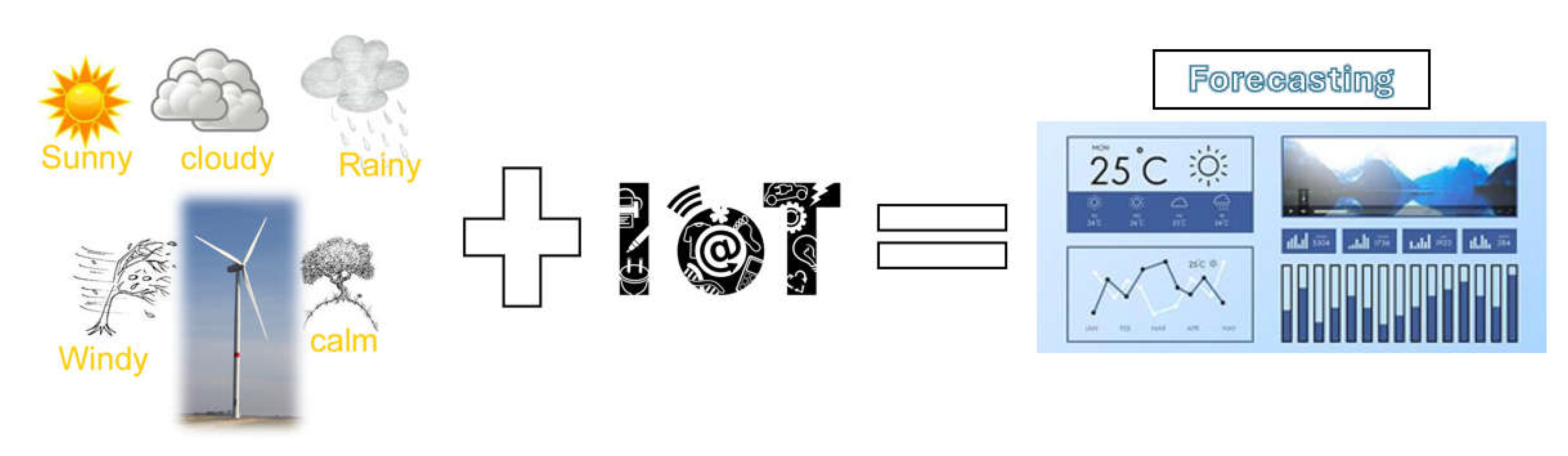
Figure 2.
Utilization of an IoT network to transfer data from turbines to the control center.
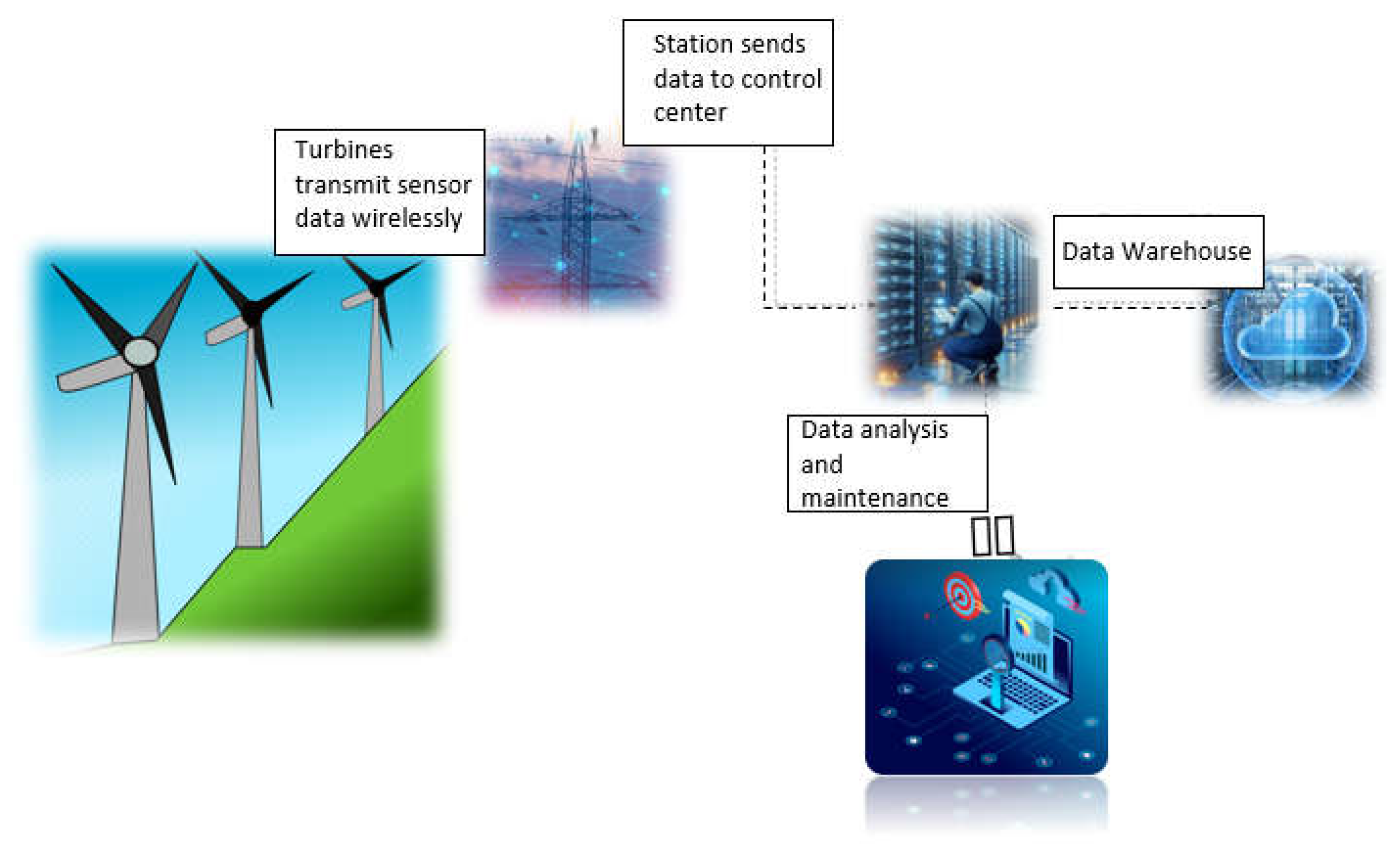
Figure 3.
Figure 3. Wind turbine components.
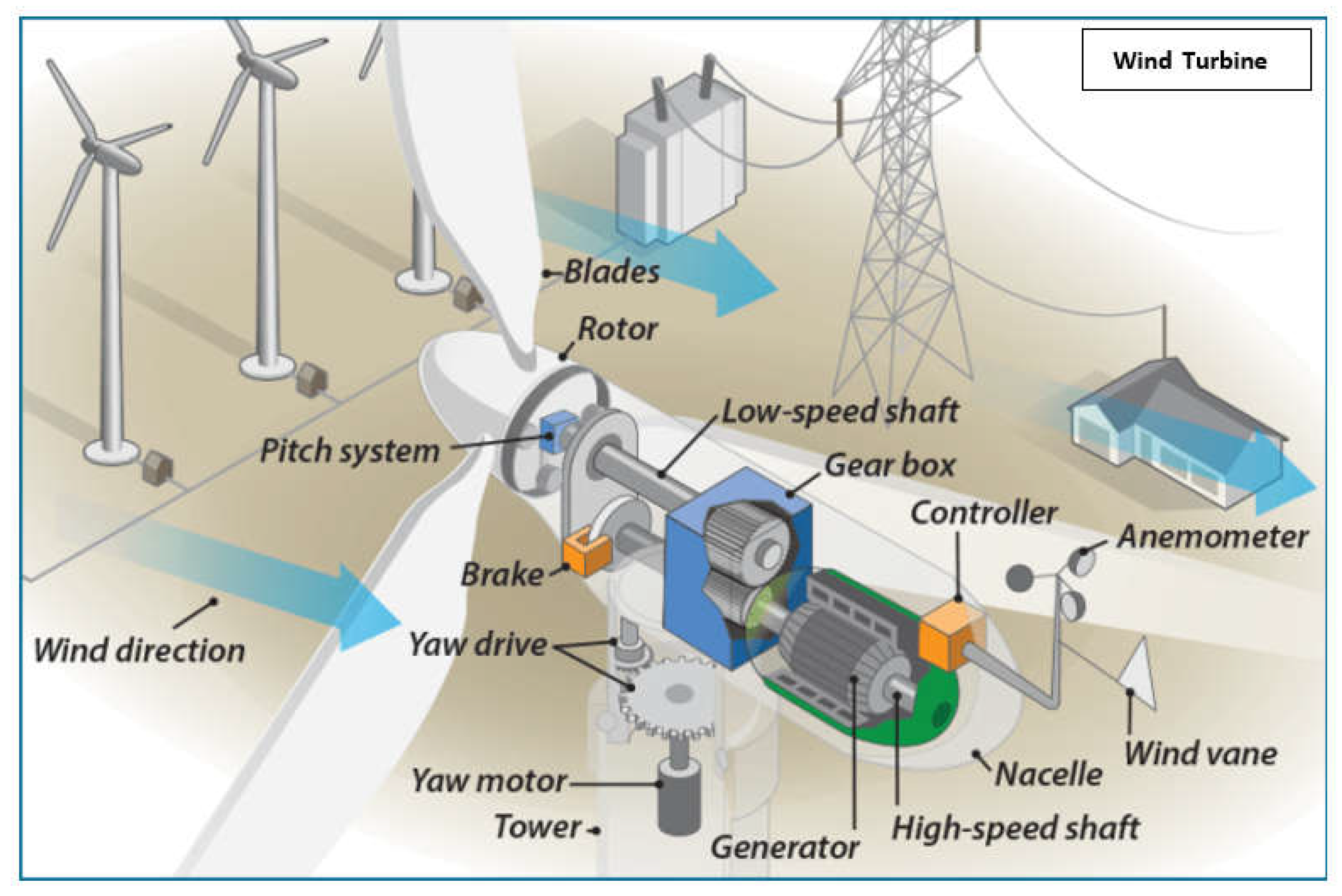
Figure 4.
Cyber layer implemented in a wind farm.
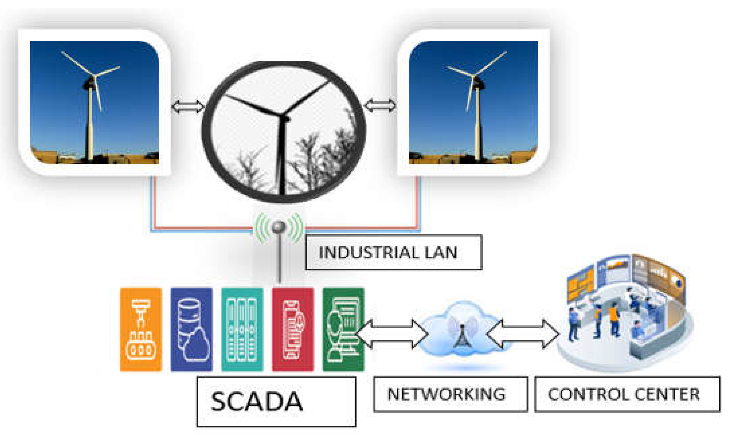
Figure 5.
Communication architecture for a wind turbine equipped with multiple sensors.
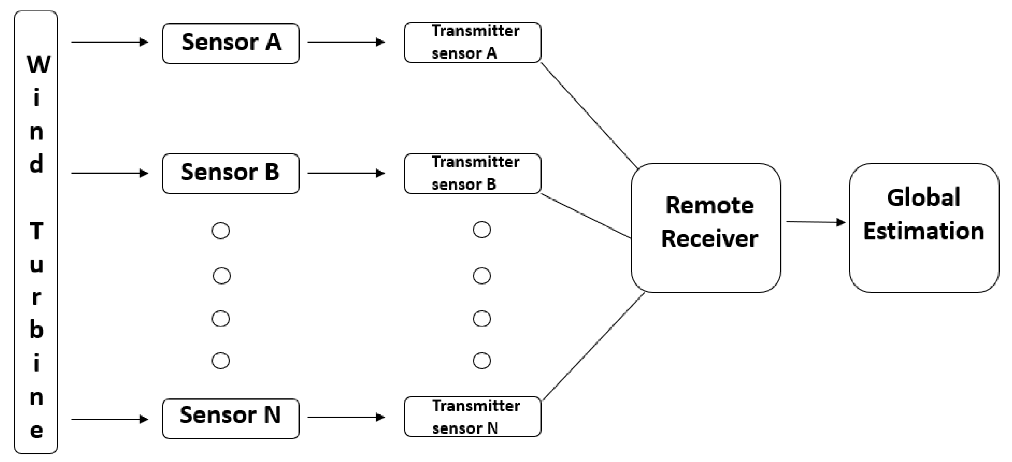
Figure 6.
CP integration of WECS.
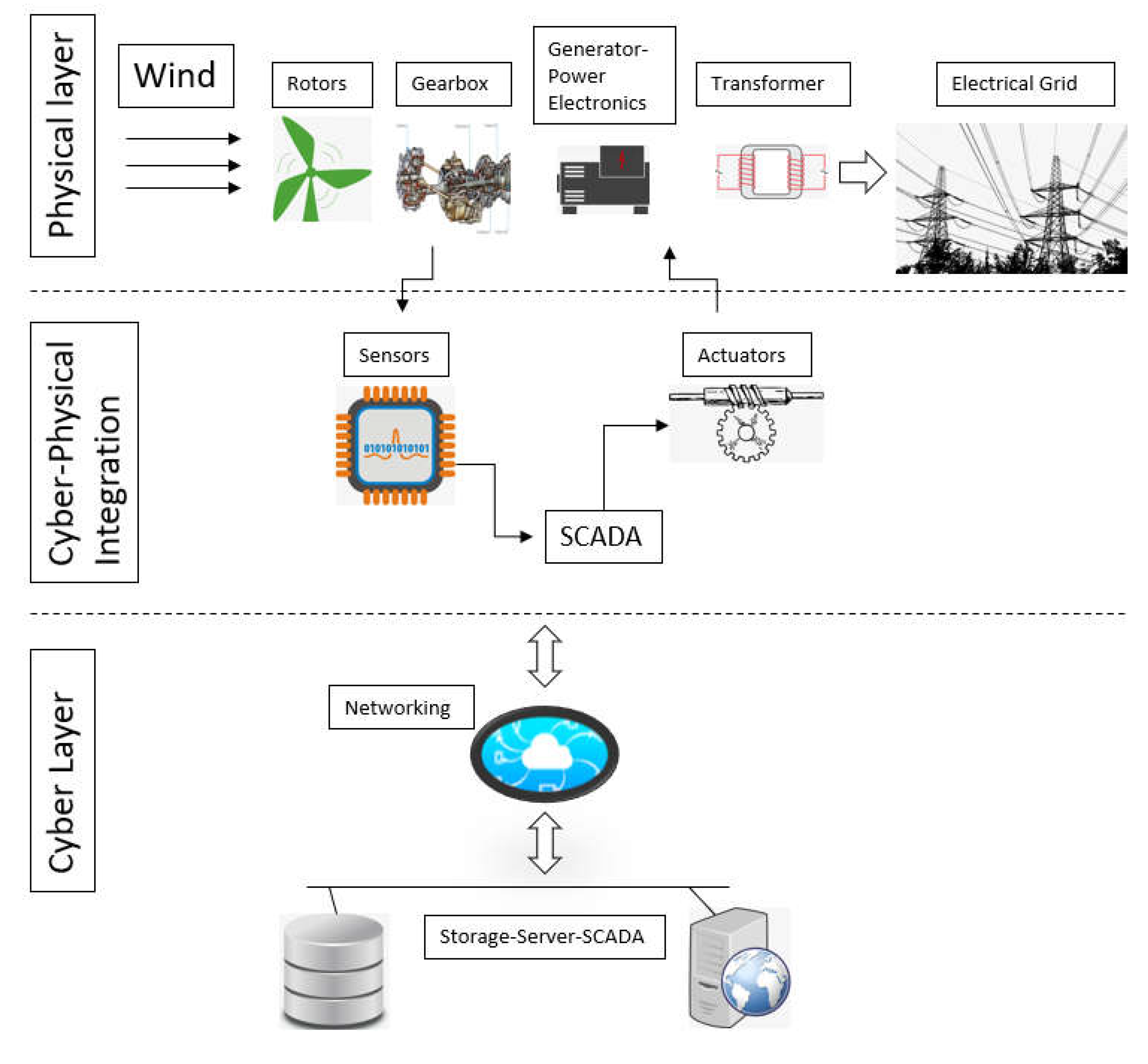
Figure 7.
The objectives of upcoming SCADA systems for WECS.
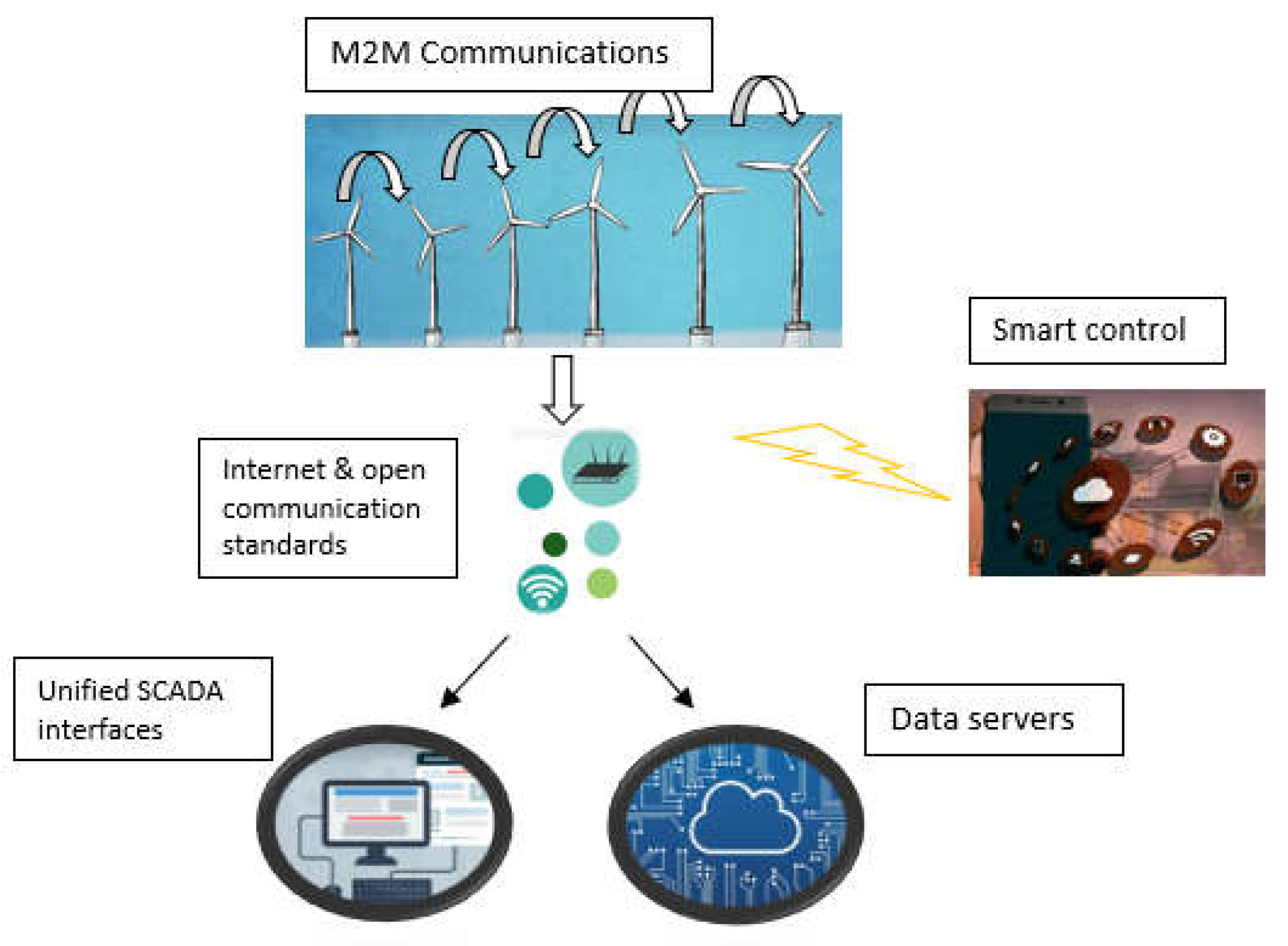
Figure 8.
Employing meteorological data to predict electric energy levels.
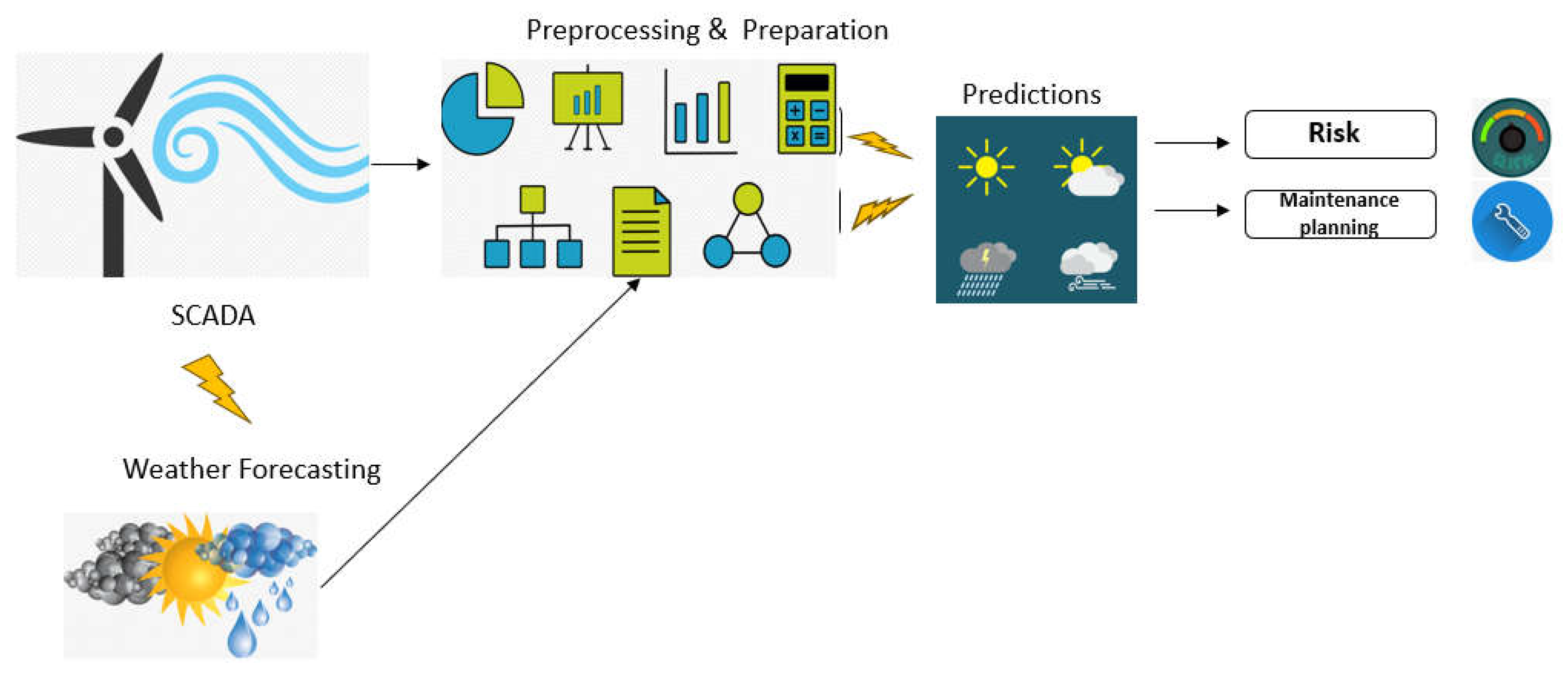
Figure 9.
Gaussian distribution including outliers.
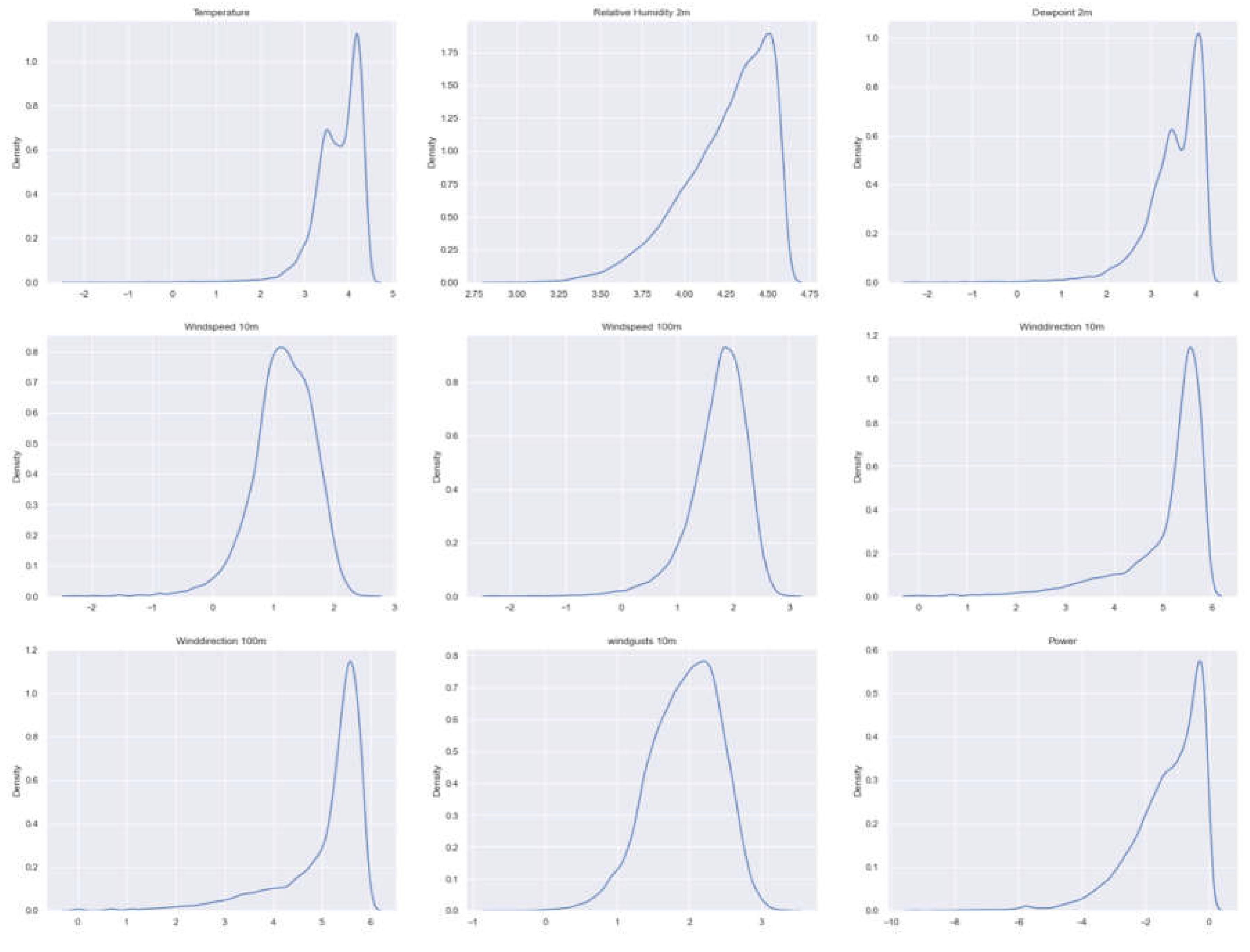
Figure 10.
The first 5 rows in Dataset of location1.
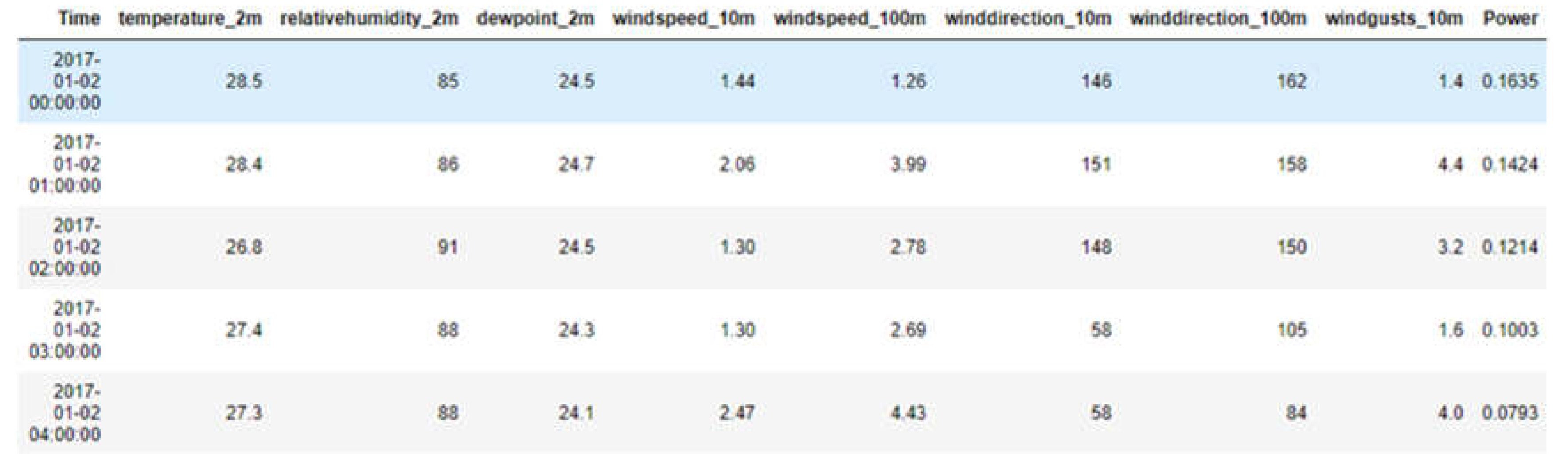
Figure 11.
Box plots for numeric columns (Time, Year, Month no needed to plot).
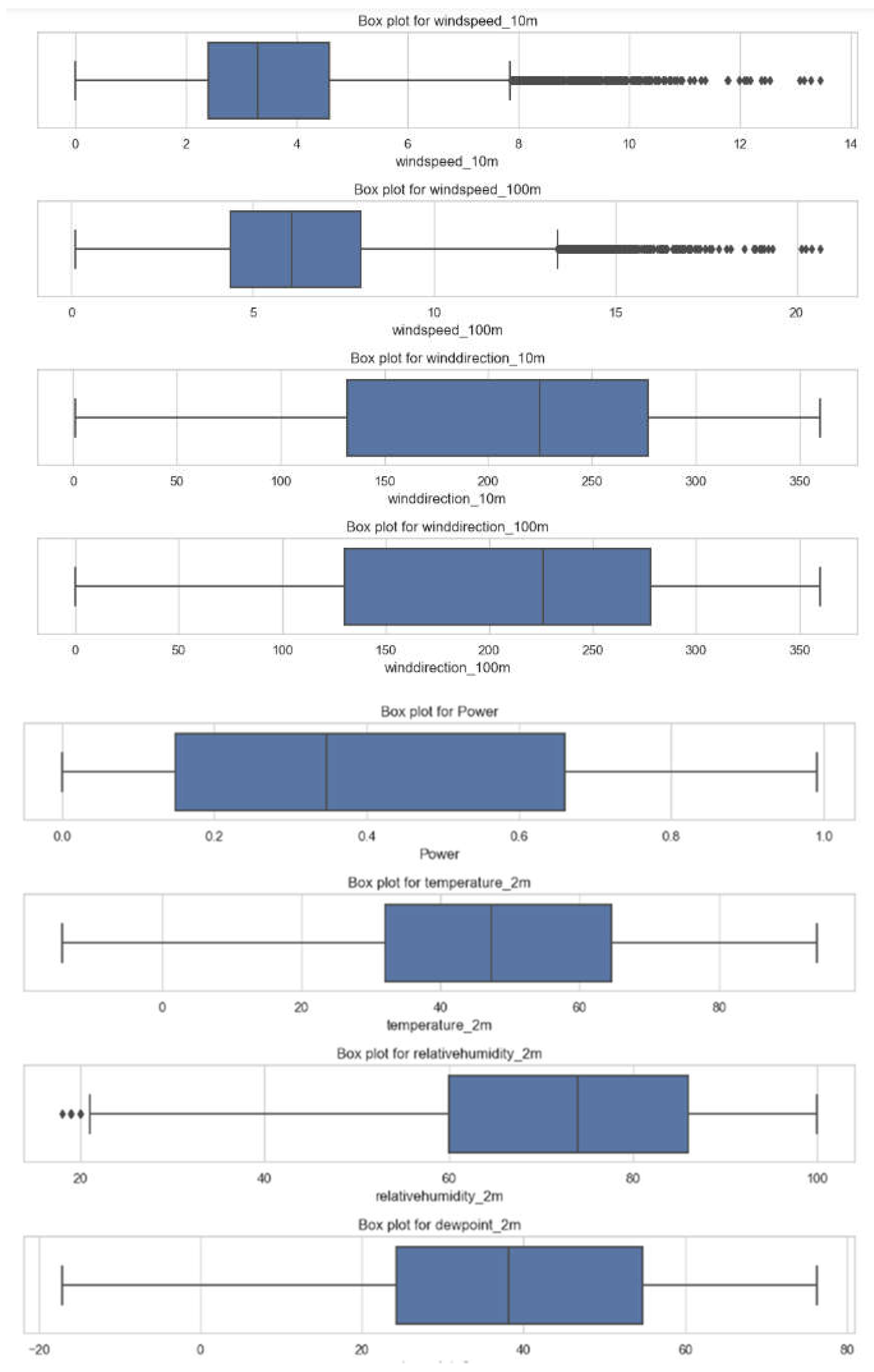
Figure 12.
Distribution of wind gusts (a) before and (b) after removal of outliers.
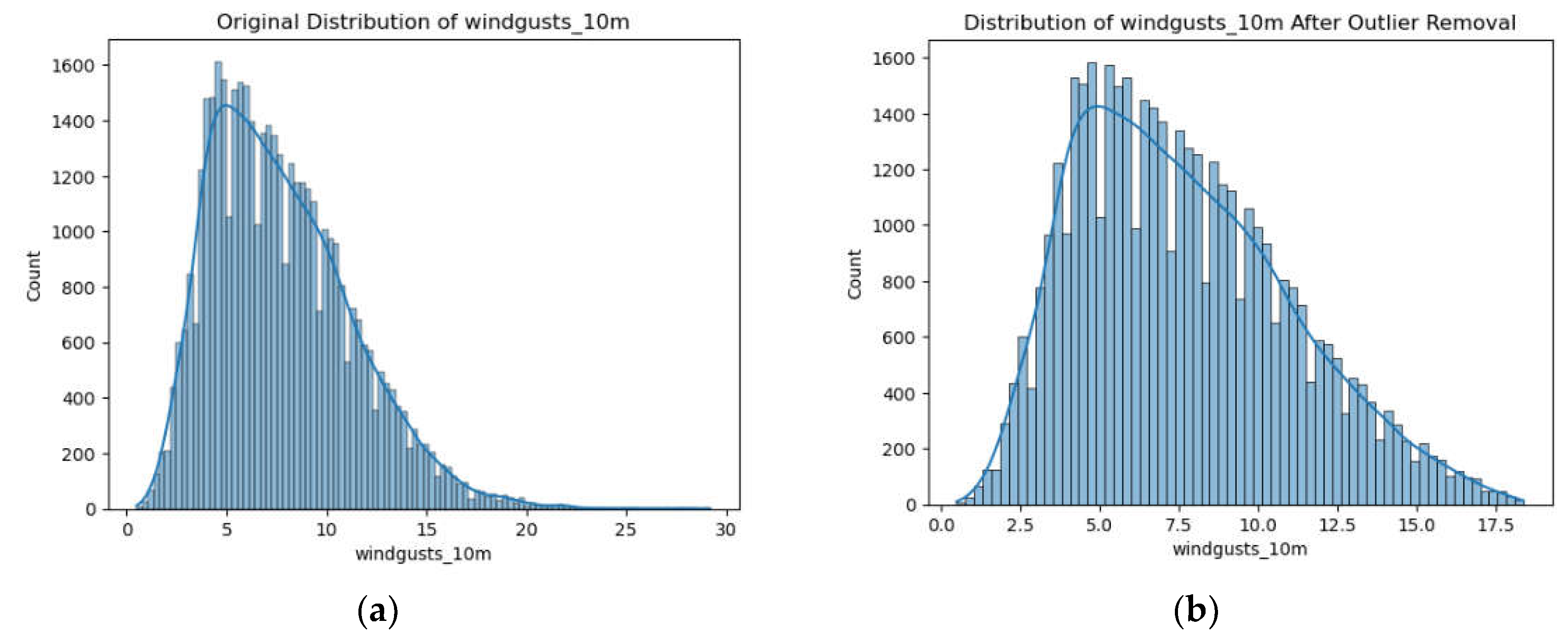
Figure 13.
Heatmap – Correlation Matrix.
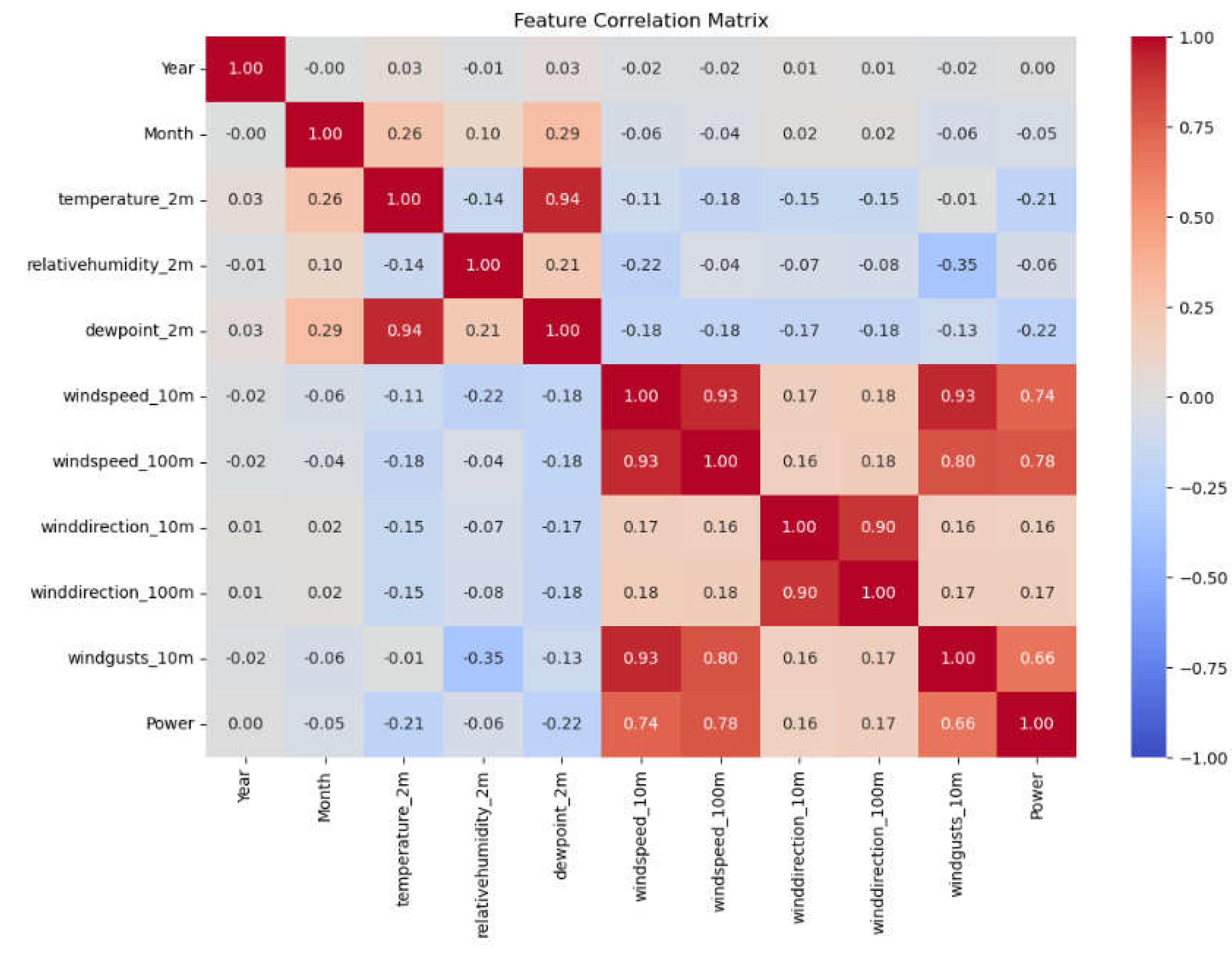
Figure 14.
Diagram of K-Fold forward Cross-Validation.
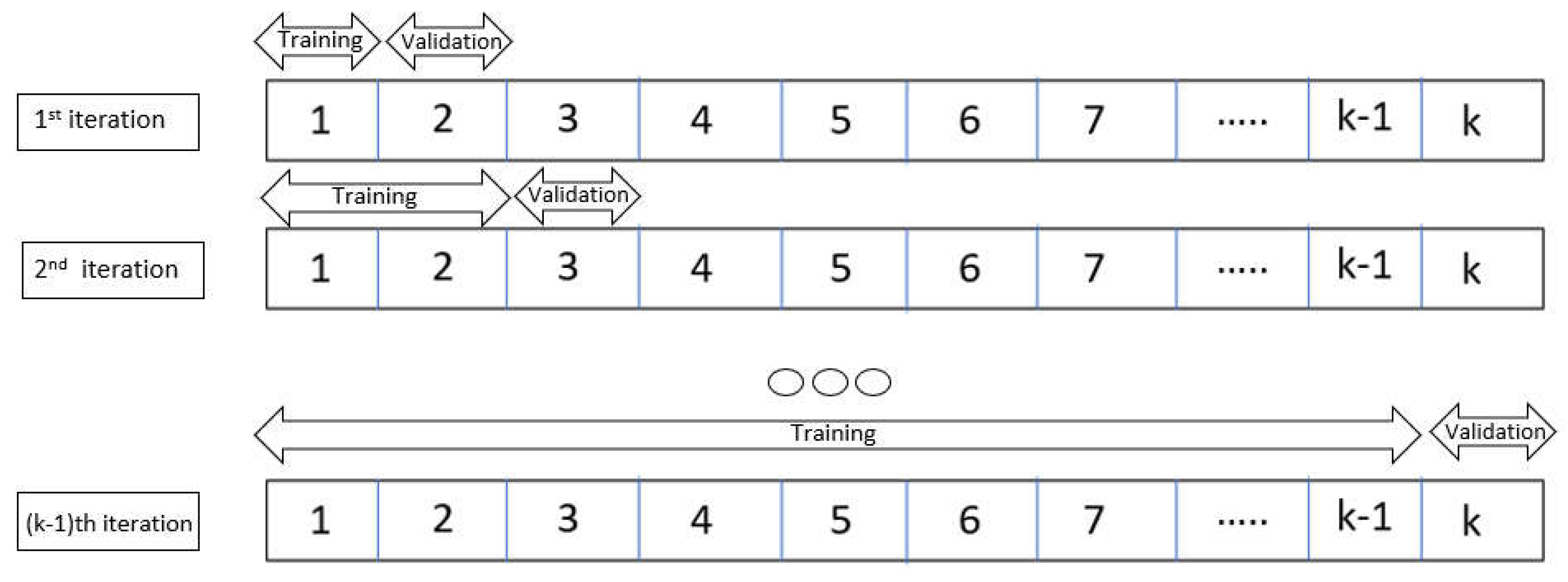
Figure 15.
(a) Actual vs. Predicted values, (b) Residual vs. Predicted values.
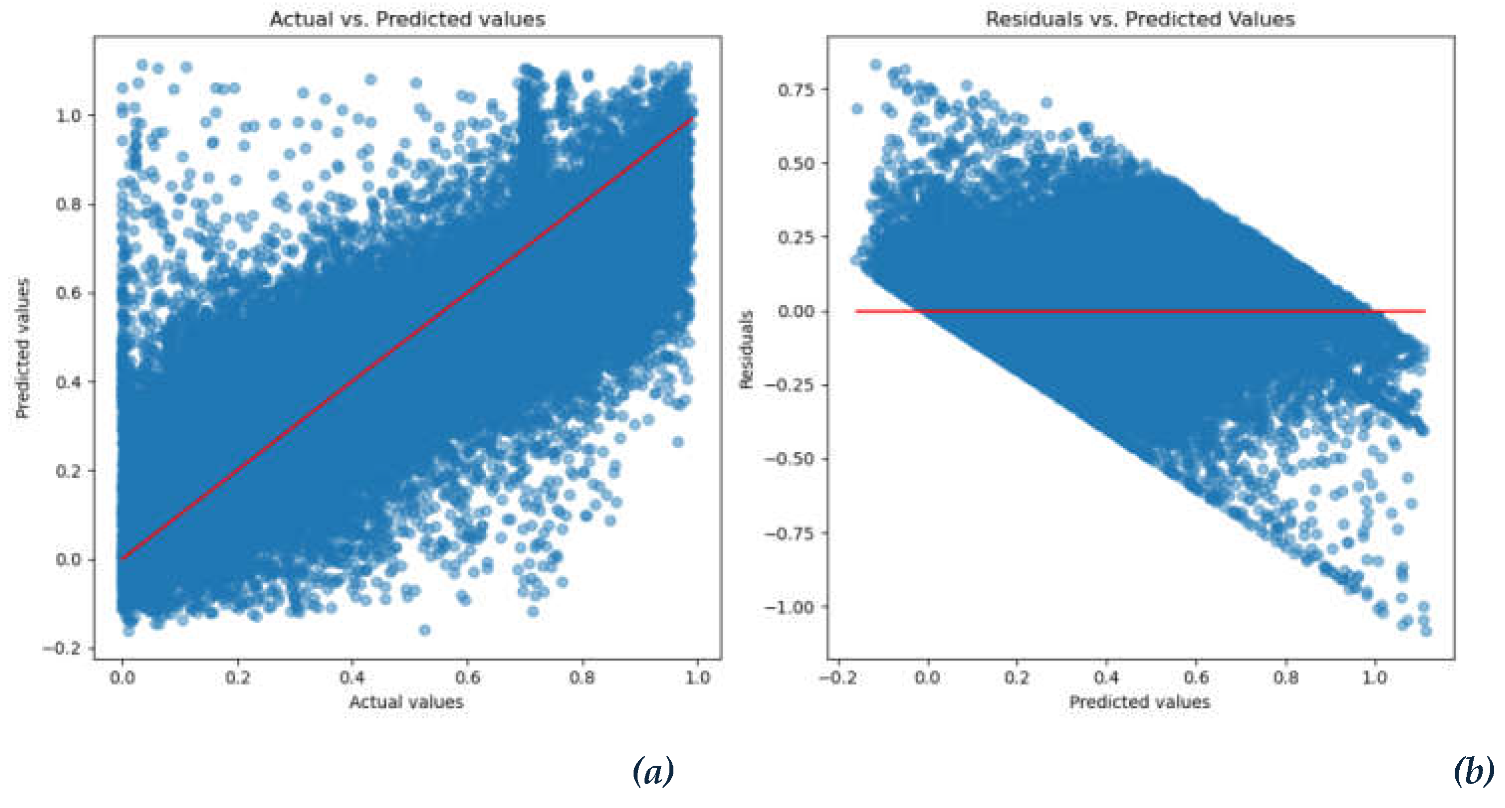
Figure 16.
Comparison of Regression Models by metrics (R2 and Adjusted R2).
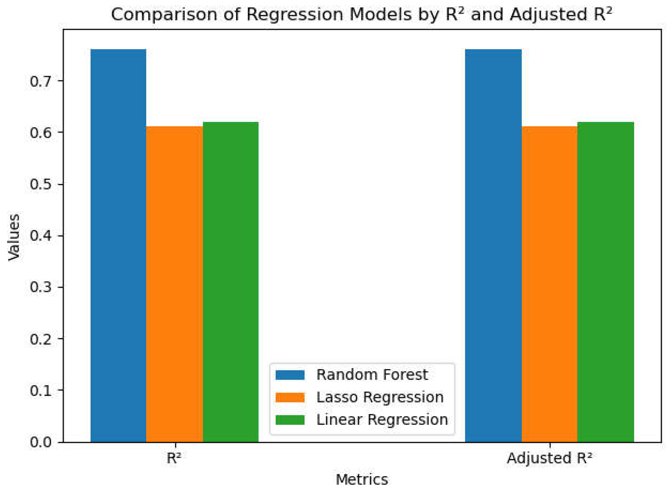
Figure 17.
Comparison of Regression Models by metrics (RMSE, MAE, MSE).
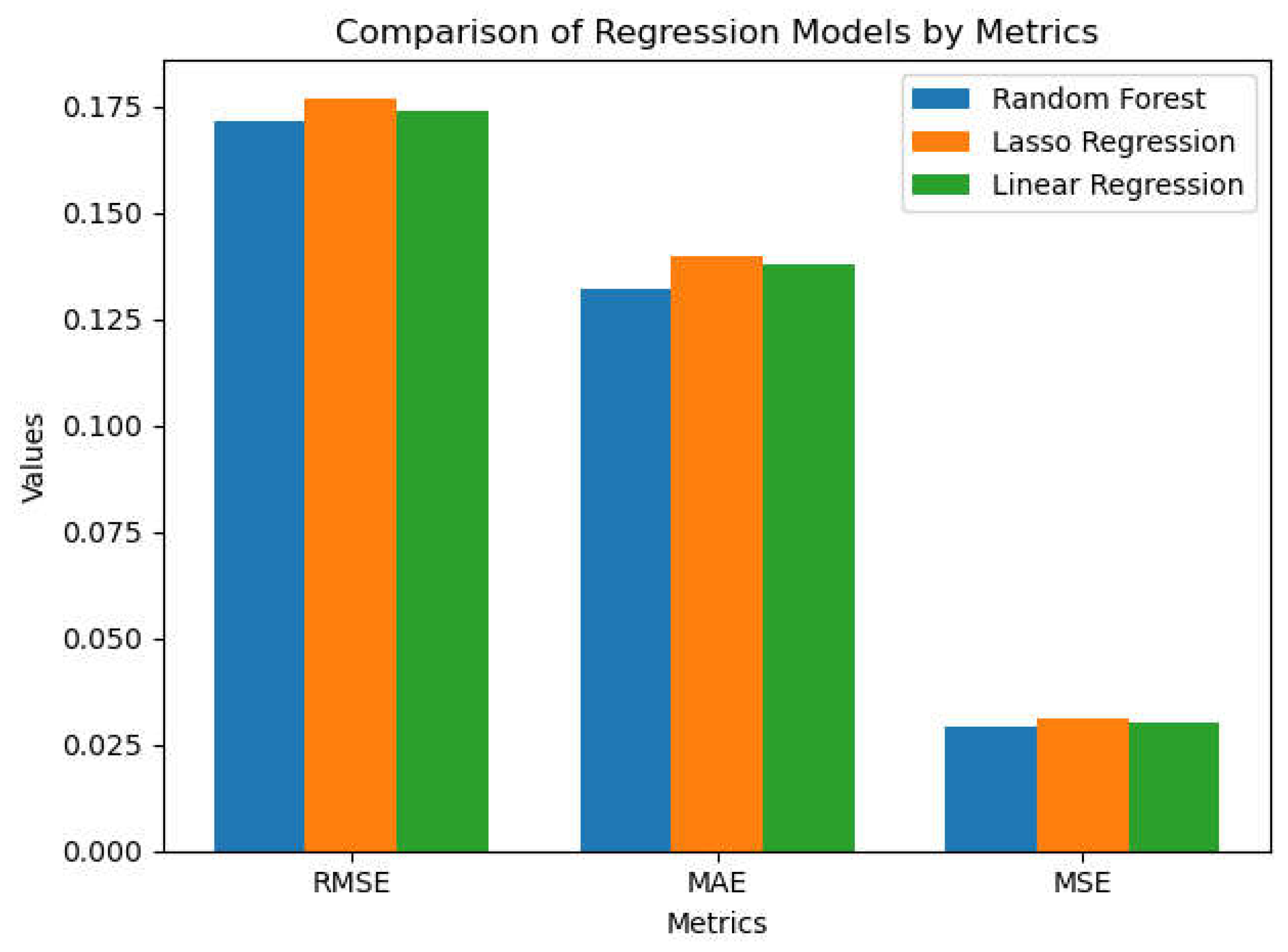

Table 1.
Data columns from location 1.
| Columns | Null values |
|---|---|
|
Time temperature_2m |
43800 non-null datetime64 43800 non-null float64 |
|
relativehumidity_2m dewpoint_2m windspeed_10m windspeed_100m winddirection_10m winddirection_100m windgusts_10m Power Year Month Day |
43800 non-null int64 43800 non-null float64 43800 non-null float64 43800 non-null float64 43800 non-null int64 43800 non-null int64 43800 non-null float64 43800 non-null float64 43800 non-null int32 43800 non-null int32 43800 non-null object |
Table 2.
Null values in the Dataset.
| Columns | Null values |
|---|---|
| temperature_2m | 0 |
| relativehumidity_2m dewpoint_2m windspeed_10m windspeed_100m winddirection_10m winddirection_100m windgusts_10m Power Year Month |
0 0 0 0 0 0 0 0 0 0 |
Table 3.
Removed outliers from columns.
| Columns | Removed Outliers |
|---|---|
| temperature_2m | 5 |
| relativehumidity_2m dewpoint_2m windspeed_10m windspeed_100m winddirection_10m winddirection_100m windgusts_10m Power Year Month |
11 0 318 199 0 0 337 Not included Not included Not included |
Table 4.
Comparison of metrics of three regression models.
| Models | R2 | Adjusted R2 | MSE | RMSE | MAE |
|---|---|---|---|---|---|
| Linear Regression | 0.6199 | 0.6194 | 0.0303 | 0.1741 | 0.1376 |
| Random Forest Regression | 0.7608 | 0.7606 | 0.0294 | 0.1715 | 0.1320 |
| Lasso Regression | 0.6110 | 0.6108 | 0.0313 | 0.1769 | 0.1399 |
Disclaimer/Publisher’s Note: The statements, opinions and data contained in all publications are solely those of the individual author(s) and contributor(s) and not of MDPI and/or the editor(s). MDPI and/or the editor(s) disclaim responsibility for any injury to people or property resulting from any ideas, methods, instructions or products referred to in the content. |
© 2024 by the authors. Licensee MDPI, Basel, Switzerland. This article is an open access article distributed under the terms and conditions of the Creative Commons Attribution (CC BY) license (http://creativecommons.org/licenses/by/4.0/).
Copyright: This open access article is published under a Creative Commons CC BY 4.0 license, which permit the free download, distribution, and reuse, provided that the author and preprint are cited in any reuse.


