
Submitted:
26 September 2024
Posted:
29 September 2024
You are already at the latest version
Abstract
Robotic exoskeletons are being actively applied to support the activities of daily living (ADL) for patients with hand motion impairments. In terms of actuation, soft materials and sensors have opened new alternatives upon conventional rigid body structures. In this arena, biomimetic soft systems are playing an important role for modeling and controlling the human hand kinematics without the restrictions of rigid mechanical joints, while having an entire deformable body with limitless points of actuation. In this paper, we address the computational limitations for modeling large-scale articulated systems for soft robotic exoskeletons, by integrating a parallel architecture to compute the exoskeleton’s dynamics equations of motion (EoM), obtaining a computation with O(log2n) complexity for the highly-articulated n degrees of freedom.
Keywords:
soft-exoskeletons
; parallel computing
; embedded systems
; HIL
; dynamics contro
1. Introduction
Exoskeletons are emerging as effective tools for facilitating motor rehabilitation in patients with impaired upper limb function [1,2]. In this regard, robotic exoskeletons designed specifically for the hand have the potential to enhance hand rehabilitation and assist individuals in activities of daily live (ADLs). The human hand poses a significant challenge for the design and control of such devices, due to its high bio-mechanical complexity [3,4]. The hand can perform precise manipulation tasks, thanks to the coordinated action of 27 bones, 27 joints, and 34 intrinsic and extrinsic muscles.
Hand exoskeletons commonly mimic the skeletal structure of the fingers, the phalanges, by means of joint-based rigid-bodies. Recently, the use of soft materials has been proposed, as they allow for more natural movements and better adaptation to the hand dexterity. The main efforts on soft exoskeletons have focused on deformable materials and real-time control of an increased number of degrees of freedom (DoF) [5,6,7,8]. However, robust closed-loop control strategies are difficult to apply since most of these methods require the calculation of the exoskeleton dynamics to compute the control signal in real-time. Among the control models for exoskeletons, position-based and force-based controls are widely used. Additionally, control strategies based on the evaluation of electromyographic (EMG) signals, combined with machine learning algorithms are increasingly proposed [9,10,11]. More recently, electroencephalographic (EEG) signals and cameras have also been proposed for motor control [12]. For instance, in [13], a rigid-soft combined mechanism is developed to support hand rehabilitation based on a EEG brain-controlled switch implemented in Matlab™, while an external VICON™motion capturing system is required to determine the fingers position in 3D space. The authors in [14] present a force myography (FMG) to allow grasping assistance. The controller is based on a switching algorithm to properly modulate a soft-extra-muscle (SEM) glove, while machine-learning models running offline were trained to estimate grasp forces. Approaches in [11,15,16] depend on machine-learning offline processing to support EEG/EMG control, force-based control or simple switch-driven modulation.
In terms of actuation, pneumatics actuators (PAs) [17], electroactive polymers (EAP) [18] and shape memory alloys (SMAs) [19] are the most predominant technologies used in soft robotic exoskeleton and gloves. As mentioned in [11,18], in most of the cases, finite elements methods (FEMs) are used to model flexible and deformable properties, requiring compute-intensive requirements. In previous efforts reported in [20,21], we presented the development of a rigid-body robotic exoskeleton to assist in the recovery of hand motor function for post-stroke subjects. Our study proposed a closed-loop model predictive control (MPC) method with the aim of compensating the effects of muscle fatigue during the rehabilitation therapies. To this purpose, EMG-based muscular effort must be detected within the control loop in order to modulate the exoskeleton’s velocity accordingly. Since the MPC method requires the computation of the exoskeleton dynamics model, applying this control algorithm implies significant challenges to soft exoskeleton mechanisms. In fact, few works in the literature [22] have applied robust control methods to modulate a soft robotic exoskeleton.
In this paper, we tackle the challenge of calculating the exoskeleton’s equations of motion (EoM) to support robust dynamics control for a hybrid soft-exoskeleton design based on compliant joints, as depicted in the inset of Figure 1a. We have adopted the parallel structure introduced by [23] to solve large-scale EoM dynamics as a foundation of the proposed soft-based highly-redundant joint exoskeleton robot. The proposed dynamics control method via inverse-dynamics EoM is based on the well-known Recursive Newton-Euler Algorithm (RNEA), presented by [24]. Figure 1b details the multi-body diagram to represent each digit of the exoskeleton. Spatial operators for velocity (), acceleration () and force () led to six-dimensional physical quantities that combined the angular and linear motions of the system. The RNEA method computes two recurrences to propagate the aforementioned spatial operators from the exoskeleton’s base to each fingertip of the serial-chain. In this regard, solving the inverse-dynamics via the RNEA method allows for the calculation of applied forces to properly control the exoskeleton’s dynamics motion. Other works in [25,26,27] have used similar approaches to dynamics modeling and robust control for exoskeletons based on the RNEA method. Nonetheless, to the best of our knowledge, this is the first work to apply a parallel solution for the RNA as an alternative to control soft exoskeletons in real-time.
As mentioned, classical techniques used in soft-robotics that are mostly based on finite element theory are not suitable in our application, since we require online computation of the dynamics model within a closed-loop control algorithm capable to scale up. To this purpose, hardware-based parallel computation of the EoM will be processed within an embedded system with multi-core CPU/GPU capabilities, to support the real-time calculation of the exoskeleton’s large-scale dynamics model, considering up to degrees of freedom to emulate continuous flexible soft bending, and achieving a computational complexity. To support the evaluation of this approach, we propose a hardware-in-the-loop (HIL) architecture as represented in Figure 1a. This control scheme consists of two main components: (i) a software-side modeling the soft-exoskeleton under analysis, which is supported by Matlab®, directly running on a desktop computer; and (ii) a hardware-side supported by an embedded platform with highly parallel computing capabilities, in charge of calculating the inverse dynamics control to drive the exoskeleton.
By adopting this HIL-based architecture, it is possible to represent very complex models, such as the referenced soft-exoskeleton, without the necessity of actually building it and integrating all the required sensors and acquisition stages. Nonetheless, this approach also allows us to validate the proposed control scheme in real hardware platforms, such as the selected embedded systems. The software-side reproduces all the complex dynamics of the exoskeleton and generates the corresponding outputs (position, velocity and acceleration) that are sent to the hardware-side. With these signals coming from the exoskeleton’s digital twin, the hardware-side applies the corresponding control scheme and in turn generates the control signals to the virtual actuators (e.g., motors), also implemented in the software-side. As it has been explained before, the biggest advantage is the ability to test, validate and evaluate the performance and scalability (with respect to the number of available cores or processing units) of the control scheme as it would execute in a real deployment. Our main contributions can be summarized as follows:
- an alternative approach to calculate dynamics equations of motion for soft exoskeletons in real-time, adopting a parallel computation for highly-articulated systems with a computational complexity, and
- the integration and deployment of this approach on embedded systems, facilitating modular dynamics-based control of soft exoskeletons by following a hardware-in-the-loop (HIL) approach.
The rest of the paper is organized as follows: Section 2.1 briefly introduces several design approaches for the proposed soft exoskeleton, based on previous works reported in [20,21,28]. Also, the formulation for the equations of motion (EoM) based on the Newton-Euler formalism using spatial operators; Section 2.2 details the proposed parallel computing approach for the EoM, by applying the well-known RNEA method (Recursive Newton-Euler Algorithm) [24,25], allowing dynamics control of the soft exoskeleton with a computational performance ; Section 3 presents the computing results obtained from several multi-core CPU/GPU embedded systems running under a HIL approach; Section 4 deals with discussions and remarks about the proposed approach for controlling soft exoskeletons; and Section 5 concludes this work with some insights, limitations and future work.
2. Methods
Our first design approach for the exoskeleton was presented in previous works reported in [20,21]. The system was conceived as a branched physical model, in which each finger is composed by a chain of rigid bodies serially connected through joint links. Figure 2a details the former mechanical design. As mentioned, we are working on a novel design approach supported by a hybrid soft mechanism based on compliant joints, as shown in Figure 2c. In order to apply our proposed method to model such mechanism, we require to determine a sufficient amount of joints to emulate soft motion properties. Figure 2b details this approximation to a soft finger of the exoskeleton via 512 degrees of freedom.
2.1. Equations of Motion
Soft motion is described based on Newton-Euler dynamics extended to large-scale articulated systems. Equations of Motion (EoM) are presented using spatial operators in , allowing joint kinematics and dynamics calculations to mimic soft deformation. Next subsection reviews the fundamental concepts of the classic mechanics that are related to body dynamics modeling, establishing an appropriate mathematical representation of the physical quantities involved in the dynamics behavior of the robotic exoskeleton.
Assuming from Figure 1b that the joint frame i and the center of mass () are two points located on the body i, the term is the position vector connecting frames i and , while connects consequently joint frames that are serially coupled. Also, the term is the rotation matrix that relates frames with . The translational () and angular velocities () for each body, as well as and forces () and moments () acting on the joint frame can be integrated into spatial operators that led to six-dimensional physical quantities, by combining the angular and linear variables of body motions. Using spatial notation, velocities V, accelerations , and forces F of a body i are expressed with respect to center of mas using six-dimensional vectors in , as follows:
Using the position vector , shown in Figure 1b, the physical quantities can be also expressed with respect to the joint frame , as:
Being the spatial operator connecting both frames, defined by the skew-symmetric matrix , as:
Where is the identity operator. From Equation (2), the spatial forces acting onto the joint frame () can be derived as , where is the spatial inertia operator of the body i with respect to its center of mass (), and corresponds to the spatial velocity defined in Equation (2). Differentiating as a function of time yields:
Using the spatial operation for translation defined in Equation (3), spatial forces with respect to the joint frame can be calculated as:
Since each finger of the exoskeleton is composed by a serial chain of connected joints, spatial forces can be propagated from the fingertip () to the base (), by using specific operators for rotation and translation. Therefore, a propagated term can be included into Equation (6), such as:
Equation (7) describes a backward propagation of spatial forces, where six-dimensional operators in for rotation R and translation P are defined as follows:
Where is the classical basic rotation matrix and is the skew-symmetric matrix of the position vector . As depicted in Figure 1b, spatial forces are calculated by following a backward propagation, initiating at the fingertip frame () and finalizing at the base frame of the exoskeleton’s finger (). To this purpose, the spatial terms in Equation (4) allow the propagation of the spatial forces (F) through the exoskeleton, considering the external load () imposed by the hand or any manipulated object. Therefore, .
Applying a similar approach, both and are also used to propagate spatial velocities () and accelerations () by following a forward propagation from , as:
The mathematical expressions for the Equations of Motion (EoM): spatial velocities , accelerations and forces are presented in Equation (7) and (9) respectively, and consolidated in Algorithm 1. The inputs to the algorithm are the joint trajectories (therapy motion) determined by the terms , whereas the output is the required torque for each joint i. As mentioned, the method is divided into two recurrences: (i) a forward calculation and propagation of the spatial velocities and accelerations and (ii) a backward recurrence to calculate spatial forces and the torques acting on each joint of the fingers. Table 1 presents the list of parameters used for the EoM. Nonetheless, this approach is insufficient to model large-scale soft systems composed by thousands of joints that enable body deformation, since the computing time increases linearly as a function of the number of degrees of freedom n.
| Algorithm 1 RNE serial computation |
|
2.2. Parallel Computing
Embedded systems with multi-core CPU/GPU architectures has enabled an increase in computational power that allows complex algorithms to run on the edge in real-time. This novel edge computing paradigm can be applied to our system, allowing a modular and compact design for the exoskeleton’s control electronics. In this regard, we propose a reformulation of Algorithm 1 to compute the EoM in a parallel fashion.
As previously mentioned, the classical formulation of the EoM based on the spatial Newton Euler formalism requires an computational complexity. It was [30] that improved the computational efficiency by computing the EoM recursively (forward dynamics) by referring the forces to generalized coordinates in the joint space. This was called the Recursive Newton-Euler Algorithm (RNEA), which was later modified by [31], by using a new approach called CRBA (Composed Rigid Body Algorithm). In [32] presented the first parallel approach to solve the CRBA for both inverse/foward dynamics problems with an complexity, but strictly dependent on the overlapping costs associated to calculation of the inertial operators. In [23], the overlapping costs of Fijany’s parallel approach was solved, adapting the RNEA algorithm by following the well-known Kogge and Stone recursive doubling technique [33].
Here, we adopted the solution proposed by [23], in order to solve the inverse dynamics model to compute the exoskeleton’s EoM into two computational recurrences: i) a forward propagation of spatial velocities (V) and accelerations (), ii) a backward propagation of spatial forces (F). Applying the Kogge and Stone method for each recurrence yields the structure presented in Figure 3, which reduces the equation set of Equation (7) and (9) for a total of computational steps (e) by powers of 2. The key element for this parallel approach is to identify the dependent term of each equation, which can be propagated to each computer node/process of the embedded system.
Note in Equation (9), the spatial velocity is composed by two terms: , in which can be propagated whereas can be computed in parallel for each computer node at the same computational step (e). The left plot of Figure 3 illustrates this process. While the serial Algorithm 1 would require computational steps to solve equations for the spatial velocities , the parallel approach solves the same equations in only computational steps, since . Likewise, spatial accelerations follow the same structure. In the case of the spatial forces, the propagation is backwards, as detailed by the right plot of Figure 3.
Therefore, scaling up to higher degrees of freedom (n), e.g. will required only computational steps, assuming the embedded systems incorporates 512 processing nodes/cores (p), i.e. . If , multi-threading can be applied for the parallel computation of the EoM. Algorithm 2 presents the parallel computation of the dynamics equations of motion for the soft exoskeleton.
In order to evaluate the performance of Algorithm 2, the Amdahl’s law is used [34]. Equation (10) describes the speedup metric, which is defined by the fraction of the algorithm that is inherently serial () and the portion that is parallelized ():
if the load distribution of processor (p) can be assigned to each individual joint of the exoskeleton (n: degrees of freedom). Otherwise, if communication packing and multi-threading processing are required.
| Algorithm 2 RNE parallel computation |
|
3. Results
Algorithm 2 was coded in ANSI C programming language and implemented using the standard message-passing-interface (MPI) supported by the mpich library [35]. In this section, we analyze the performance of the RNE algorithm running in several computing architectures:
- Intel®Core™i7 Processor with 6 CPU cores at 2.6GHz and 512 GPU NVIDIA Quadro P1000 cores | 32GB RAM | Ubuntu 22.04.3 LTS.
- Hardware-in-the-loop (HIL) with the Embedded Nvidia Jetson™Nano with 1024 cores at 625MHz | 8GB RAM | Ubuntu 22.04.3 LTS.
Figure 4 details the computing time response of the proposed parallel approach running on the Intel®Core™i7 with NVIDIA Quadro GPU. The plot Figure 4a compares both serial and parallel algorithms. As mentioned, both solutions for the inverse dynamics EoM were coded in ANSI C, using the high-performance Meschach framework; a comprehensive matrix-vector linear algebra for the operation of 6D spatial terms. The RNE approach significantly outperformed the serial algorithm DoF, obtaining a real-time response of in the calculation of the inverse dynamics control for the soft exoskeleton with joints. In this test, we used an interpolated 3D spline trajectory with knot-points. Contrary, the serial RNE required for the calculations. Considering the size of the input trajectory for the exoskeleton ( knot-points), the net computational time is proportional to . In this sense, the inset within plot Figure 4b shows the resulting computing time of the parallel RNE approach with variations in the input trajectory knot-points.
The overall performance of the proposed solution is presented in Figure 5. The speedup exponentially increases after , while achieving a degree of parallelism after approximately , which demonstrates the required scalability for controlling highly-articulated and large-scale soft exoskeletons in real-time.
Another important element of the proposed RNE algorithm is related to the propagation structure of the EoM, in which the inherent sequential-time component of the algorithm can be drastically reduced if an embedded system-on-chip (SoC) is used. With an SoC-based embedded system, CPU/GPU cores are integrated with the memory in the same silicon, allowing higher data bandwidth to propagate data. This issue can be observed in Figure 6. Using the MPICH-library jumpshot feature, real execution with data propagation can be analyzed, by determining both serial and parallel computing time involved the calculation of the dynamics EoM. In this test, we used to clearly visualize the computational steps (e) followed by the propagation of spatial velocities (), accelerations () and forces (), as previously defined in Figure 3.
As previously mentioned, classical techniques used in soft-robotics that rely on finite element theory are not suitable in our application, since we require real-time computation running online while the exoskeleton. In this regard, we compared our RNE model against the Ansys®simulator, performing finite element analysis based on the Newton-Raphson iteration method applied to the proposed semi-soft structure driven by the compliant joint mechanism shown in Figure 2c. Also, as detailed in the inset of Figure 7a, the exoskeleton model is composed by one finger with 3 phalanges (the distal, middle, and proximal) performing a closing/opening trajectory with 90 knot-points with a step time of . Under this topology Ansys used nodes for the semi-soft structure of the exoskeleton, requiring a simulation time of and execution time of . Ansys determines the number of nodes and degrees of freedom (DoF) automatically. For the same trajectory with knot-points and a step time of , our RNE model required for 512 DoF, as shown in Figure 4b. Increasing up to DoF yielded a computing time of , using a MPI configuration for (more degrees of freedom than processing cores). Even with this computing-intense configuration, our model dramatically outperformed Ansys results in terms of simulation time.
Also, Figure 7b presents computing time results for the soft model implemented in SoRoSim©Matlab™introduced by [29]. SoRoSim uses Geometric Variable Strain (GVS) approach for the dynamic simulation of soft systems. We tested several configurations from up to joints for the links assembly, as detailed in the insets of Figure 7b. For , the method performed with a computational time of , whereas our method required . Besides, the computational performance of SoRoSim exhibits a linear complexity , i.e., higher computing times will be obtained for large-scale articulated soft systems, compromising the scalability of the solution. In contrast, our model will scale with a complexity of , as demonstrated in Figure 4.
Next, we present the performance of the RNE algorithm running in a SoC-based embedded system with 1024 cores powered by the Nvidia Jetson Orin™Nano, with the ultimate goal of reducing the inherent serial time computation of Algorithm 2, and the advantage of compacting the proposed inverse-dynamics controller to support closed-loop robust control of the soft exoskeleton in real-time by following the proposed Hardware-in-the-loop (HIL) configuration. Figure 8 presents the experimental results obtained with this embedded system.
Both mpich and meschach libraries were compiled within the Nvidia Jetson Orin™Nano, allowing the computation of Algorithm 2 with similar computing times of those obtained from the Intel®Core™i7 Processor with 512 GPU NVIDIA Quadro cores, as presented in Figure 4b. For , the parallel RNE algorithm required for trajectory knot-points. As observed in Figure 8, the variance in computational time remains under , resulting feasible for in-loop real-time response.
Finally, Table 2 presents the computing time results for the aforementioned tests: refers to Algorithm 1 running on the Intel®Core™i7 Processor with 512 GPU NVIDIA Quadro cores, SoroSim refers to the tests presented in Figure 7b running under Matlab™, also refers to Algorithm 2 running on the Intel®Core™i7 Processor, whereas HIL- refers to Algorithm 2 running on the embedded Nvidia Jetson Orin™Nano with 1024 cores. Furthermore, for the tests conducted in Ansys®, was not possible to configure the soft exoskeleton for different DoF values, since Ansys®determined DoF for the assembly shown in Figure 7a, requiring a simulation time of ( minutes).
4. Discussion
Algorithm 2 was implemented and tested on the embedded Nvidia Jetson Orin™Nano with 1024 cores, allowing the real-time calculation of the proposed inverse-dynamics controller based on the RNE method. As shown in Figure 8, the obtained computational complexity is of the form , being the overall knot-points used to interpolate the reference trajectory for the exoskeleton.
In this regard, it is worth to highlight that those changes in the trajectory knot-points are associated with the precision and intensity of the therapy. In previous work reported in [28], we used a VICON™ motion capture system to extract the kinematics of motion associated to 6 hand gestures for rehabilitation. We implemented interpolation methods based on 3D splines to determine both cartesian and joint trajectories to drive the exoskeleton assistance. Here, the joint trajectory for positions (), velocities () and accelerations () are used as inputs to Algorithm 2, in order to estimate the computing time cost of the parallel inverse dynamics controller by analyzing the impact of increasing motion precision according to the computational complexity of the form .
Although similar computing times were obtained with the embedded platform in comparison to the desktop solution (c.f Table 2), the proposed HIL-driven embedded approach allow us to deploy a modular control system, facilitating the use of the soft exoskeleton in real rehabilitation scenarios. Also, we demonstrate that even with higher values of , the inherent logarithmic response is maintained, supporting highly-articulated soft exoskeletons.
5. Conclusions
Classical finite element methods used in soft-robotics are not suitable for the real-time computation of model-dependent non-linear controllers, since most control algorithms require the dynamics calculation of the EoM within the closed-loop. As an alternative, our approach relies on the well-known Recursive Newton-Euler Algorithm (RNEA) calculated in a parallel fashion. As a result, a hardware-in-the-loop (HIL) structured allowed us to compute the proposed inverse-dynamics controller, by following a computational performance. Real-time response was achieved by testing our model on the Nvidia Jetson Orin™Nano embedded system, enabling to close the control-loop in ( for the hybrid soft-exoskeleton mechanism depicted in Figure 2c.
The EoM presented in Algorithm 1, allows us to incorporate external forces and perturbations for the robotic exoskeleton, that can be generated by the patient during real rehabilitation scenarios. Our non-linear control method based on the inverse-dynamics RNE is able to counteract these perturbations, as shown in step 3 from Algorithm 1, being the term the external payload to overcome with the control law . Here, we have demonstrated that this control output can be generated in real-time thanks to the parallel computation of Algorithm 2.
Author Contributions
Conceptualization, J. Colorado, D. Mendez; methodology, J. Colorado, D. Mendez, Andres Gomez-Bautista, John Bermeo, Fredy Cuellar; software, J. Colorado, Andres Gomez-Bautista, John Bermeo, Fredy Cuellar; validation, J. Colorado, D. Mendez, Andres Gomez-Bautista, John Bermeo, Fredy Cuellar; formal analysis, J. Colorado, D. Mendez, Andres Gomez-Bautista, John Bermeo, Fredy Cuellar, C. Alvarado-Rojas; investigation, J. Colorado, D. Mendez, C. Alvarado-Rojas; data curation, J. Colorado, Andres Gomez-Bautista; writing—original draft preparation, J. Colorado; writing—review and editing, D. Mendez, Andres Gomez-Bautista, John Bermeo, Fredy Cuellar, C. Alvarado-Rojas; supervision, J. Colorado, D. Mendez; project administration, J. Colorado; funding acquisition, J. Colorado. All authors have read and agreed to the published version of the manuscript.
Funding
This work was funded by the project “iREHAB: Sistema inteligente de Rehabilitación usando un Exoesqueleto para recuperar Habilidad motora en discapacidades post-ACV, usando señales Biológicas del paciente” sponsored by The Ministry of Science Technology and Innovation (MinCiencias), program 918-2022 under GRANT CTO: 622-2022, Award ID: 91805.
Data Availability Statement
Data is unavailable due to privacy or ethical restrictions.
Conflicts of Interest
The authors declare no conflict of interest.
References
- Huang, Y.; Nam, C.; Li, W.; Rong, W.; Xie, Y.; Liu, Y.; Qian, Q.; Hu, X. A comparison of the rehabilitation effectiveness of neuromuscular electrical stimulation robotic hand training and pure robotic hand training after stroke: A randomized controlled trial. Biomedical Signal Processing and Control 2020, 56, 101723. [Google Scholar] [CrossRef]
- Du Plessis, T.; Djouani, K.; Oosthuizen, C. A review of active hand exoskeletons for rehabilitation and assistance. Robotics 2021, 10, 40. [Google Scholar] [CrossRef]
- Logozzo, S.; Valigi, M.C.; Malvezzi, M. Modelling the human touch: A basic study for haptic technology. Tribology international 2022, 166, 107352. [Google Scholar] [CrossRef]
- Kladovasilakis, N.; Kostavelis, I.; Sideridis, P.; Koltzi, E.; Piliounis, K.; Tzetzis, D.; Tzovaras, D. A Novel Soft Robotic Exoskeleton System for Hand Rehabilitation and Assistance Purposes. Applied Sciences 2022, 13, 553. [Google Scholar] [CrossRef]
- Zhu, M.; Biswas, S.; Dinulescu, S.I.; Kastor, N.; Hawkes, E.W.; Visell, Y. Soft, wearable robotics and haptics: Technologies, trends, and emerging applications. Proceedings of the IEEE 2022, 110, 246–272. [Google Scholar] [CrossRef]
- Lin, L.; Zhang, F.; Yang, L.; Fu, Y. Design and modeling of a hybrid soft-rigid hand exoskeleton for poststroke rehabilitation. International Journal of Mechanical Sciences 2021, 212, 106831. [Google Scholar] [CrossRef]
- Shahid, T.; Gouwanda, D.; Nurzaman, S.G.; Gopalai, A.A. Moving toward soft robotics: A decade review of the design of hand exoskeletons. Biomimetics 2018, 3, 17. [Google Scholar] [CrossRef] [PubMed]
- Li, M.; He, B.; Liang, Z.; Zhao, C.G.; Chen, J.; Zhuo, Y.; Xu, G.; Xie, J.; Althoefer, K. An attention-controlled hand exoskeleton for the rehabilitation of finger extension and flexion using a rigid-soft combined mechanism. Frontiers in neurorobotics 2019, 13, 34. [Google Scholar] [CrossRef] [PubMed]
- Tiboni, M.; Borboni, A.; Faglia, R.; Pellegrini, N. Robotics rehabilitation of the elbow based on surface electromyography signals. Advances in Mechanical Engineering 2018, 10, 1687814018754590. [Google Scholar] [CrossRef]
- Sierotowicz, M.; Lotti, N.; Nell, L.; Missiroli, F.; Alicea, R.; Zhang, X.; Xiloyannis, M.; Rupp, R.; Papp, E.; Krzywinski, J.; others. EMG-driven machine learning control of a soft glove for grasping assistance and rehabilitation. IEEE Robotics and Automation Letters 2022, 7, 1566–1573. [Google Scholar] [CrossRef]
- Achilli, G.M.; Amici, C.; Dragusanu, M.; Gobbo, M.; Logozzo, S.; Malvezzi, M.; Tiboni, M.; Valigi, M.C. Soft, Rigid, and Hybrid Robotic Exoskeletons for Hand Rehabilitation: Roadmap with Impairment-Oriented Rationale for Devices Design and Selection. Applied Sciences 2023, 13. [Google Scholar] [CrossRef]
- Tiboni, M.; Borboni, A.; Vérité, F.; Bregoli, C.; Amici, C. Sensors and actuation technologies in exoskeletons: A review. Sensors 2022, 22, 884. [Google Scholar] [CrossRef] [PubMed]
- Li, M.; He, B.; Liang, Z.; Zhao, C.G.; Chen, J.; Zhuo, Y.; Xu, G.; Xie, J.; Althoefer, K. An Attention-Controlled Hand Exoskeleton for the Rehabilitation of Finger Extension and Flexion Using a Rigid-Soft Combined Mechanism. Frontiers in Neurorobotics 2019, 13. [Google Scholar] [CrossRef] [PubMed]
- Islam, M.R.U.; Bai, S. Effective Multi-Mode Grasping Assistance Control of a Soft Hand Exoskeleton Using Force Myography. Frontiers in Robotics and AI 2020, 7. [Google Scholar] [CrossRef]
- Asif, A.R.; Waris, A.; Gilani, S.O.; Jamil, M.; Ashraf, H.; Shafique, M.; Niazi, I.K. Performance evaluation of convolutional neural network for hand gesture recognition using EMG. Sensors 2020, 20, 1642. [Google Scholar] [CrossRef]
- Lu, Z.; Stampas, A.; Francisco, G.E.; Zhou, P. Offline and online myoelectric pattern recognition analysis and real-time control of a robotic hand after spinal cord injury. Journal of neural engineering 2019, 16, 036018. [Google Scholar] [CrossRef] [PubMed]
- Tiboni, M.; Loda, D. Monolithic PneuNets soft actuators for robotic rehabilitation: methodologies for design, production and characterization. Actuators 2023, 12, 299. [Google Scholar] [CrossRef]
- Peng, Z.; Huang, J. Soft Rehabilitation and Nursing-Care Robots: A Review and Future Outlook. Applied Sciences 2019, 9. [Google Scholar] [CrossRef]
- Copaci, D.; Blanco, D.; Moreno, L. Wearable elbow exoskeleton actuated with shape memory alloy in antagonist movement. Proceedings of the Joint Workshop on Wearable Robotics and Assistive Devices, International Conference on Intelligent Robots and Systems, Daejeon, Korea, 2016, pp. 9–14.
- Bonilla, D.; Bravo, M.; Bonilla, S.P.; Iragorri, A.M.; Mendez, D.; Mondragon, I.F.; Alvarado-Rojas, C.; Colorado, J.D. Progressive Rehabilitation Based on EMG Gesture Classification and an MPC-Driven Exoskeleton. Bioengineering 2023, 10. [Google Scholar] [CrossRef]
- Castiblanco, J.C.; Mondragon, I.F.; Alvarado-Rojas, C.; Colorado, J.D. Assist-As-Needed Exoskeleton for Hand Joint Rehabilitation Based on Muscle Effort Detection. Sensors 2021, 21. [Google Scholar] [CrossRef]
- Pal, A.; He, T.; Wei, W. Sample-efficient Model Predictive Control Design of Soft Robotics by Bayesian Optimization. ArXiv, 2022; arXiv:abs/2210.08780. [Google Scholar]
- Jaramillo-Botero, A.; Lorente, A.C.I. A Unified Formulation for Massively Parallel Rigid Multibody Dynamics of O(log2n) Computational Complexity. Journal of Parallel and Distributed Computing 2002, 62, 1001–1020. [Google Scholar] [CrossRef]
- Featherstone, R. The Recursive Newton-Euler Algorithm. In Encyclopedia of Robotics; 2020; Ang, M.H., Khatib, O., Siciliano, B., Eds.; Springer Berlin Heidelberg: Berlin, Heidelberg, 2020; pp. 1–5. [Google Scholar] [CrossRef]
- Kvrgic, V.; Vidakovic, J. Efficient method for robot forward dynamics computation. Mechanism and Machine Theory 2020, 145, 103680. [Google Scholar] [CrossRef]
- Chen, C.T.; Lien, W.Y.; Chen, C.T.; Twu, M.J.; Wu, Y.C. Dynamic Modeling and Motion Control of a Cable-Driven Robotic Exoskeleton With Pneumatic Artificial Muscle Actuators. IEEE Access 2020, 8, 149796–149807. [Google Scholar] [CrossRef]
- Gurriet, T.; Mote, M.; Singletary, A.; Nilsson, P.; Feron, E.; Ames, A.D. A Scalable Safety Critical Control Framework for Nonlinear Systems. IEEE Access 2020, 8, 187249–187275. [Google Scholar] [CrossRef]
- Arteaga, M.V.; Castiblanco, J.C.; Mondragon, I.F.; Colorado, J.D.; Alvarado-Rojas, C. EMG-driven hand model based on the classification of individual finger movements. Biomedical Signal Processing and Control 2020, 58, 101834. [Google Scholar] [CrossRef]
- Mathew, A.T.; Hmida, I.B.; Armanini, C.; Boyer, F.; Renda, F. SoRoSim: A MATLAB Toolbox for Hybrid Rigid–Soft Robots Based on the Geometric Variable-Strain Approach. IEEE Robotics and Automation Magazine 2023, 30, 106–122. [Google Scholar] [CrossRef]
- Amin-Javaheri, M.; Orin, D.E. Parallel Algorithms for Computation of the Manipulator Inertia Matrix. The International Journal of Robotics Research 1991, 10, 162–170. [Google Scholar] [CrossRef]
- Featherstone, R. A Divide-and-Conquer Articulated-Body Algorithm for Parallel O(log(n)) Calculation of Rigid-Body Dynamics. Part 1: Basic Algorithm. The International Journal of Robotics Research 1999, 18, 867–875. [Google Scholar] [CrossRef]
- Bhalerao, K.D.; Critchley, J.; Anderson, K. An efficient parallel dynamics algorithm for simulation of large articulated robotic systems. Mechanism and Machine Theory 2012, 53, 86–98. [Google Scholar] [CrossRef]
- Kogge, P.M.; Stone, H.S. A Parallel Algorithm for the Efficient Solution of a General Class of Recurrence Equations. IEEE Transactions on Computers, -22. [CrossRef]
- Gustafson, J.L. Amdahl’s Law. In Encyclopedia of Parallel Computing; 2011; Padua, D., Ed.; Springer US: Boston, MA, 2011; pp. 53–60. [Google Scholar] [CrossRef]
- Gropp, W.; Lusk, E.; Skjellum, A. Using MPI (): portable parallel programming with the message-passing interface, 2nd ed.; MIT Press: Cambridge, MA, USA, 1999. [Google Scholar]
Figure 1.
(a) Hardware in-the-loop approach to compute large-scale exoskeleton’s multi-body dynamics using parallel computing. (b) Soft articulated multi-body diagram.
Figure 1.
(a) Hardware in-the-loop approach to compute large-scale exoskeleton’s multi-body dynamics using parallel computing. (b) Soft articulated multi-body diagram.
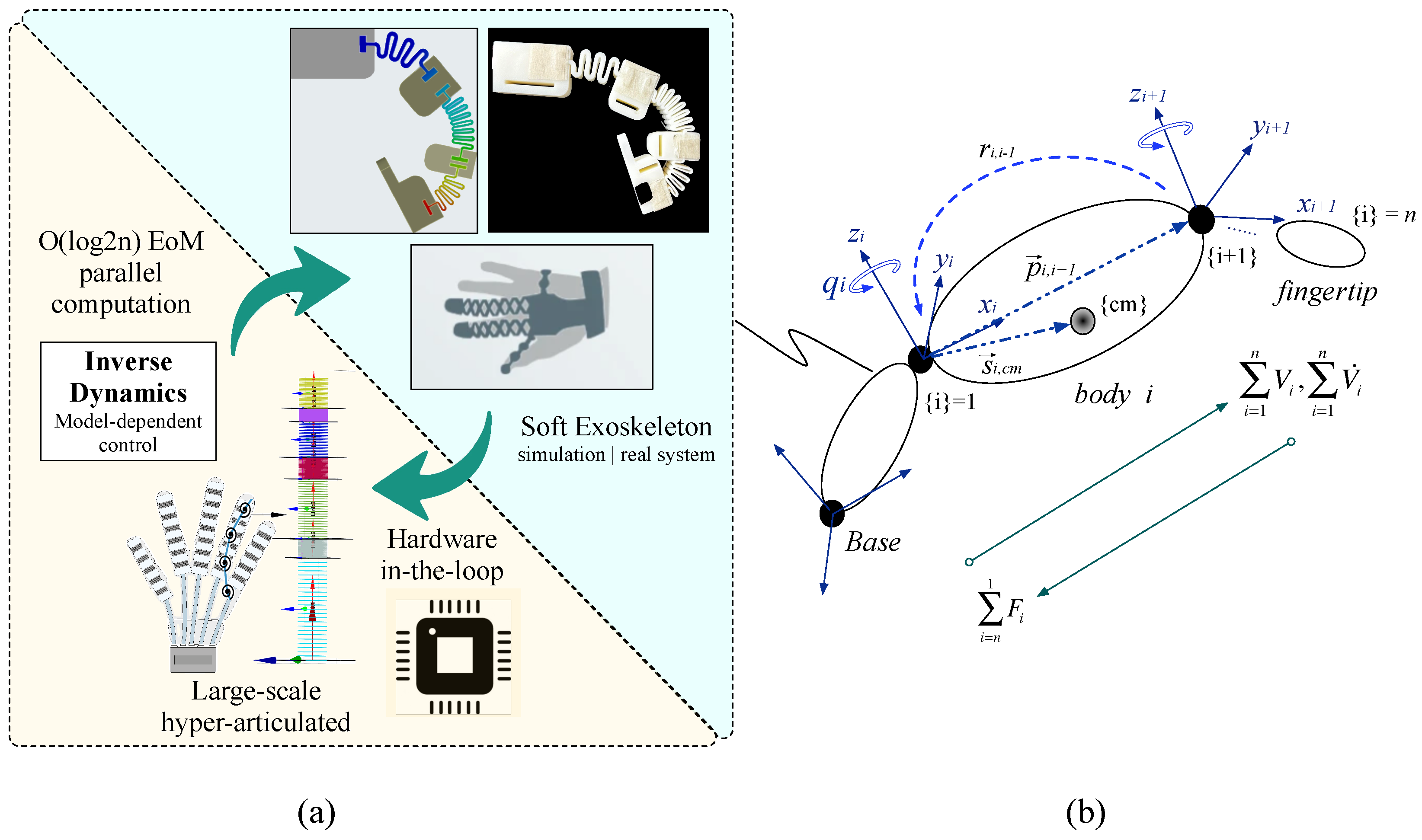
Figure 2.
(a) Former rigid-body mechanism reported in previous work in [20], composed by 3 under-actuated joints connected to a single actuation input driven by a linear actuator. (b) Soft model implemented in SoRoSim©Matlab™composed by 512 degrees of freedom that emulate flexible bending [29]. (c) Proposed novel mechanism based on a semi-soft structure driven by compliant joints.
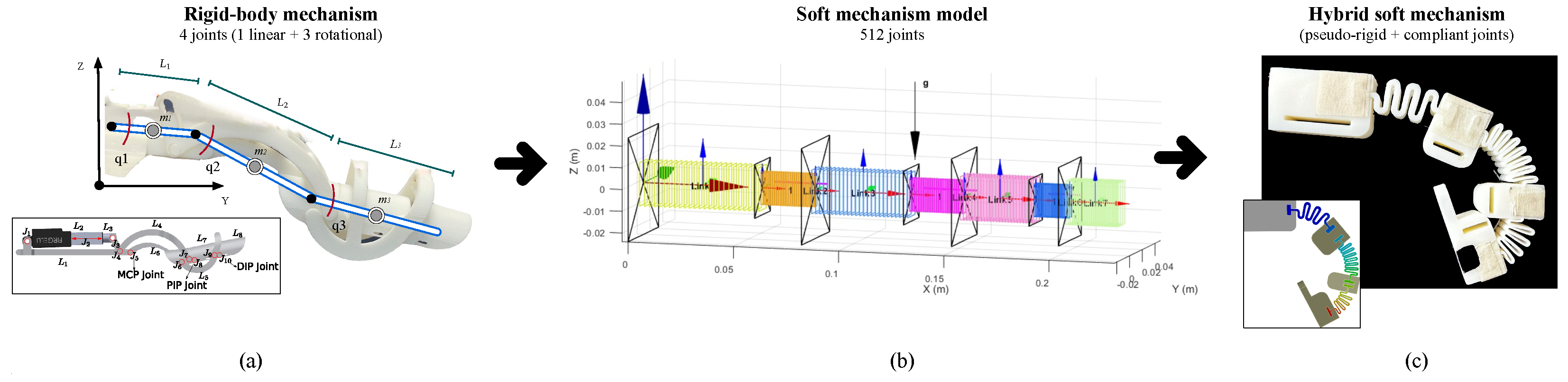
Figure 3.
Parallel EoM calculation by following a computational complexity. Computing steps (e) are depicted for the case of degrees of freedom (DoF). For higher joints (), the same propagation scheme is maintained. In the left, both spatial velocities (V) and accelerations () are computed by following a forward propagation. In the right, spatial forces (F) are calculated in a backward direction. Computing cores are represented by each node.
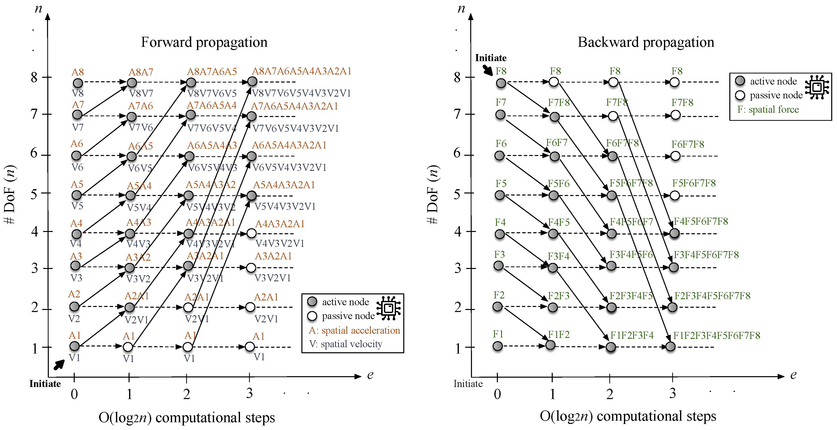
Figure 4.
(a) Computation time comparison between the serial RNE (c.f Algorithm 1) VS the parallel RNE (c.f Algorithm 2). (b) closed-up to the response of Algorithm 2) including computational time variations depending on the number of trajectory points () defined for the exoskeleton’s therapy motions. For this test, was adjusted between 500 up to trajectory knot-points with a fixed step-time of (platform: Intel®Core™i7 Processor with 512 GPU NVIDIA Quadro cores).

Figure 5.
Speedup for the proposed RNE algorithm in comparison to the Amdahl’s law for several degrees of parallelism from (platform: Intel®Core™i7 Processor with 512 GPU NVIDIA Quadro cores).
Figure 5.
Speedup for the proposed RNE algorithm in comparison to the Amdahl’s law for several degrees of parallelism from (platform: Intel®Core™i7 Processor with 512 GPU NVIDIA Quadro cores).
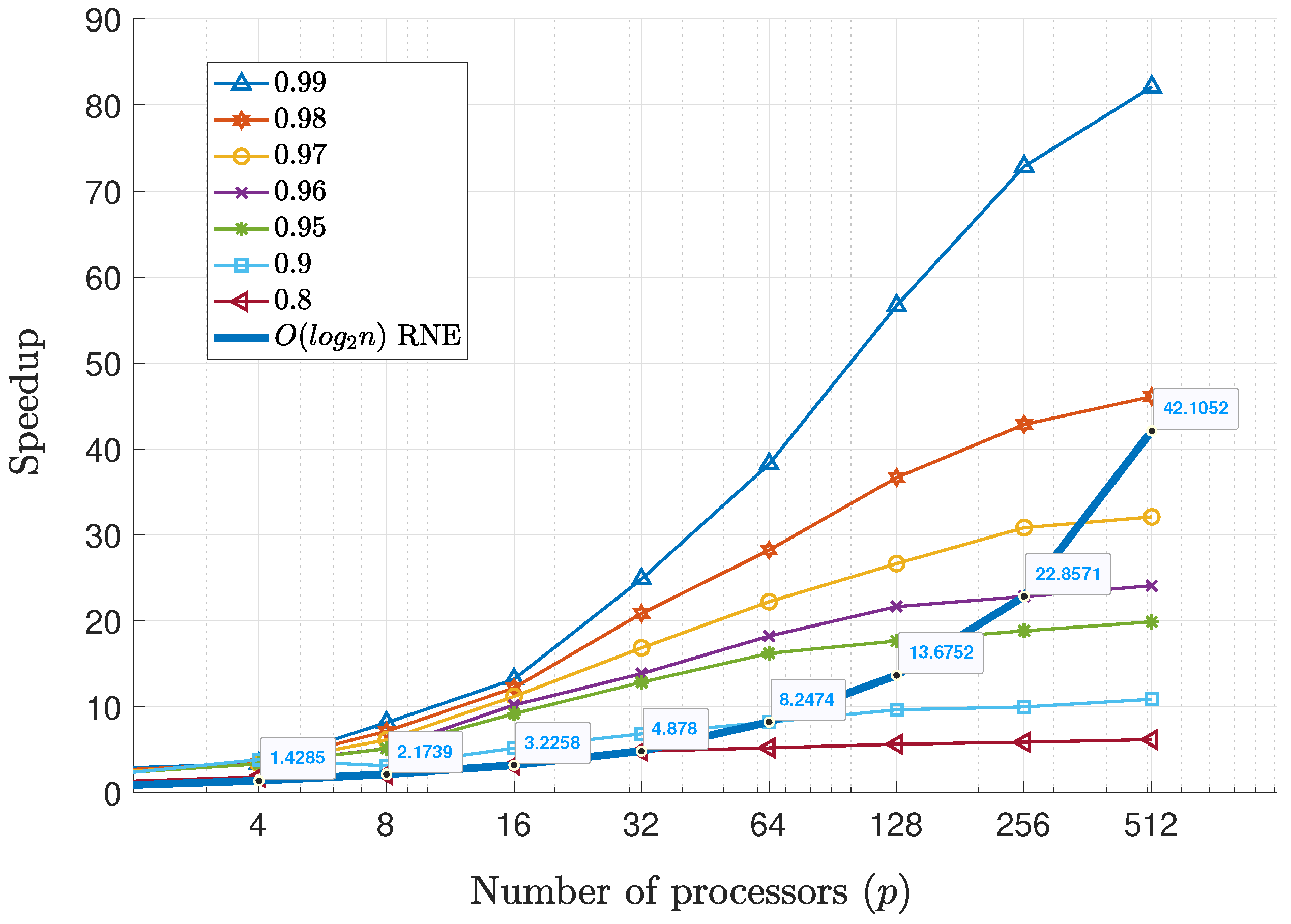
Figure 6.
Computational steps of the RNE algorithm during execution. The propagation scheme follows the structure defined in Figure 3, detailing the MPI-driven data passing between cores (): forward propagation for spatial and accelerations, followed by a backward propagation for computing spatial forces (platform: Intel®Core™i7 Processor with 512 GPU NVIDIA Quadro cores).
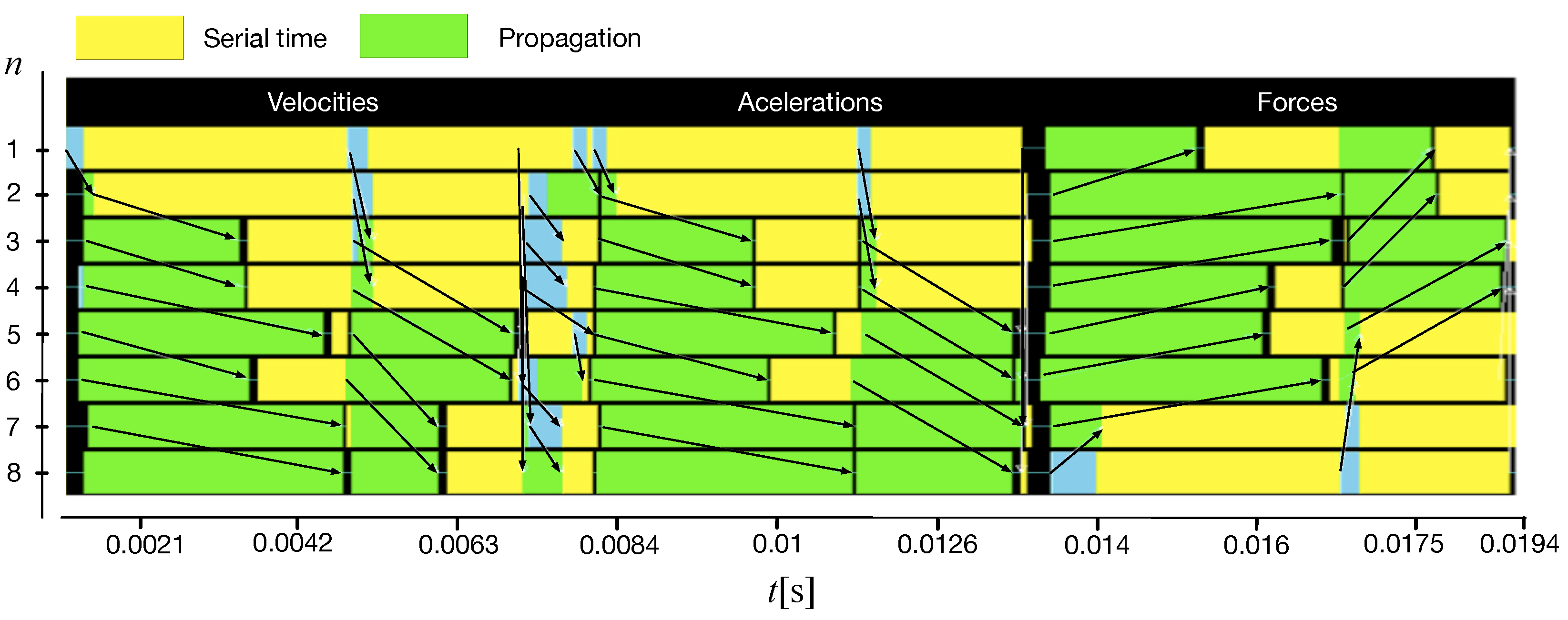
Figure 7.
(a) Ansys®simulation for the proposed semi-soft structure driven by the compliant joint mechanism. (b) Computing time for the soft model implemented in SoRoSim©Matlab™.
Figure 7.
(a) Ansys®simulation for the proposed semi-soft structure driven by the compliant joint mechanism. (b) Computing time for the soft model implemented in SoRoSim©Matlab™.
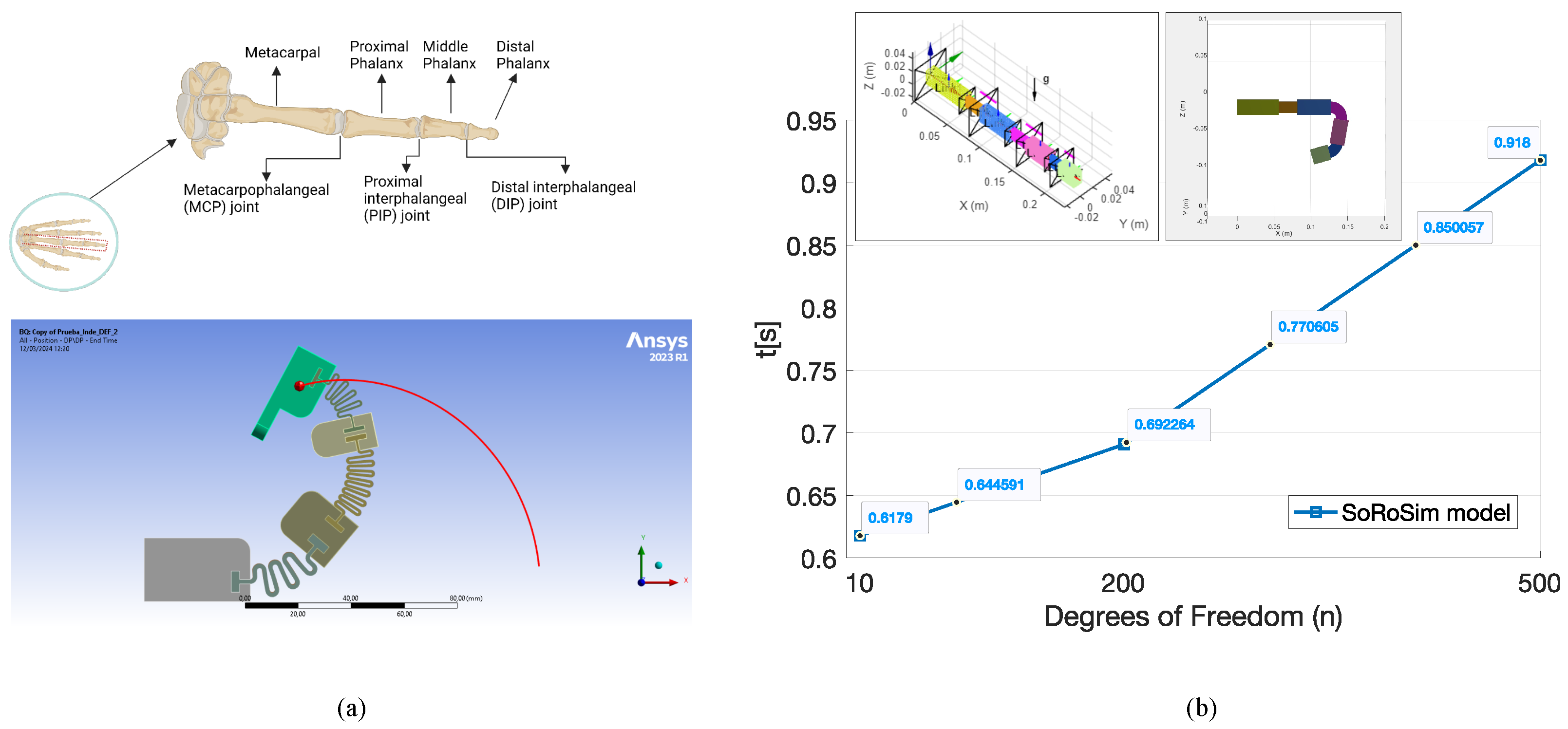
Figure 8.
HIL-based response of Algorithm 2 including computational time variations depending on the number of trajectory points (platform: Nvidia Jetson Orin™Nano with 1024 cores).
Figure 8.
HIL-based response of Algorithm 2 including computational time variations depending on the number of trajectory points (platform: Nvidia Jetson Orin™Nano with 1024 cores).
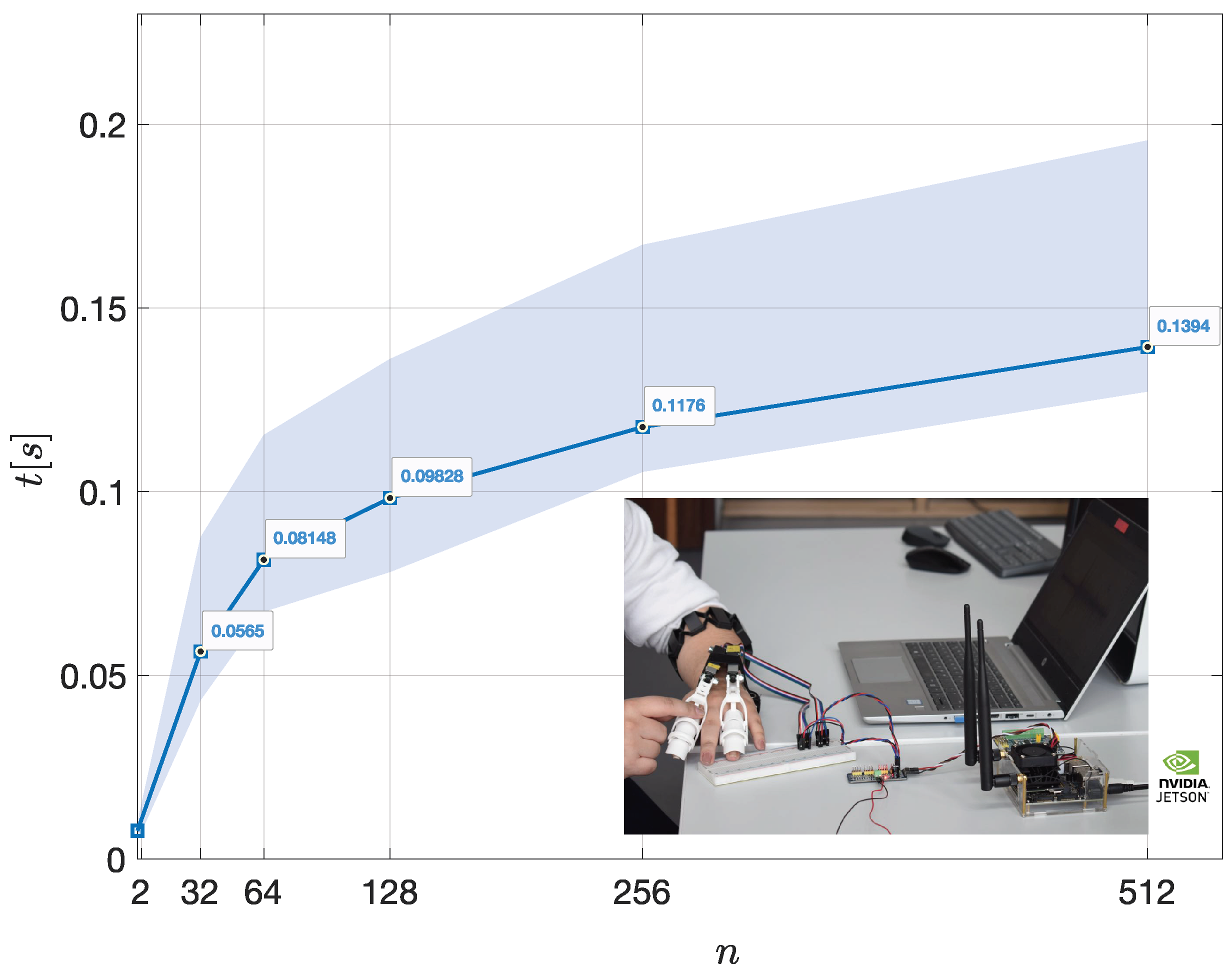

Table 1.
Parameters for the EoM in Algorithm 1.
| Parameter | Description |
| i | subscript that indicates the joint frame |
| 6D spatial velocity and acceleration of body i with respect to joint frame | |
| 6D spatial force of body i with respect to joint frame | |
| H | 6D vector for projection onto the axis of motion |
| spatial inertia of body i with respect to frame | |
| 3x1 position vector that joins frame to | |
| skew symmetric matrix of vector cross product of | |
| spatial translation from joint frame to | |
| joint positions, velocities and accelerations of body i with respect to | |
| 3x3 basic rotation matrix that projects frame onto frame | |
| spatial rotation from joint frame to | |
| 3x1 position vector that joins frame to | |
| skew symmetric matrix of vector cross product of | |
| spatial translation from joint frame to | |
| U | 3x3 identity operator |
| linear velocity and acceleration of body i with respect to joint frame | |
| angular velocity and acceleration of body i with respect to joint frame | |
| torques at joint frame |
Table 2.
Computing time comparison between platforms and methods.
| Method | n=32 | n=64 | n=128 | n=256 | n=512 |
| 0.24 | 0.58 | 1.16 | 2.33 | 4.67 | |
| SoroSim | 0.62 | 0.64 | 0.66 | 0.73 | 0.91 |
| 0.0478 | 0.0814 | 0.0982 | 0.1176 | 0.1276 | |
| HIL- | 0.0565 | 0.08148 | 0.09828 | 0.1176 | 0.13945 |
Disclaimer/Publisher’s Note: The statements, opinions and data contained in all publications are solely those of the individual author(s) and contributor(s) and not of MDPI and/or the editor(s). MDPI and/or the editor(s) disclaim responsibility for any injury to people or property resulting from any ideas, methods, instructions or products referred to in the content. |
© 2024 by the authors. Licensee MDPI, Basel, Switzerland. This article is an open access article distributed under the terms and conditions of the Creative Commons Attribution (CC BY) license (http://creativecommons.org/licenses/by/4.0/).
Copyright: This open access article is published under a Creative Commons CC BY 4.0 license, which permit the free download, distribution, and reuse, provided that the author and preprint are cited in any reuse.


