Suitable Hamiltonian for the Riemann Hypothesis: Coinciding with Heavy Atom $U _{238}$

1. Main Results

• 1) We developed a stochastic model based on the Maynard-Guth corollary to capture the stochastic nature of prime distribution in almost-short intervals. The model is defined by the following equation:

  $$x_{n+1}=x_n+{\displaystyle \frac{y}{log{x}_n}}+{ϵ}_n,$$

  (1)
  where:
• $x_n$ represents the number of primes in the n-th interval.
• y is the fixed length of the interval.
• $log{x}_n$ incorporates the influence of the prime number theorem.
• ${ϵ}_n$ is a random error term, modeled as a Laplace distribution with parameters $\mu$ and b.
  Through analysis of the stochastic properties of this model, we found that the stochastic model approximates a uniform distribution. We compared this model with the distribution of primes in almost-short intervals, demonstrating that it closely aligns with the observed prime distribution. Additionally, we compared the statistical properties of the stochastic model with the Prime Number Theorem (PNT) and achieved consistency with both models.
• 2) We investigated the statistical properties of the quantum model using the derived formulations of the associated Hamiltonian. Our analysis revealed that the energy levels of the Hamiltonian are quantized and follow a Gamma distribution. Furthermore, the probability density function (PDF) of the Hamiltonian closely resembles the Gaussian Orthogonal Ensemble (GOE) from large random matrix theory, indicating that our model shares statistical characteristics with well-known random matrix ensembles.
• 3) Our numerical experiments confirm that our new bound, associated with our stochastic model, significantly outperforms both the Walfisz and Maynard-Guth bounds, especially for large x. The new bound is highly sensitive to parameter choices, with optimal selections yielding tighter error terms and improved accuracy. Additionally, statistical comparisons show the model accurately captures higher-order moments, despite slight underestimation in the mean and variance.

  $$\left|\pi (x+y)-\pi \left(x\right)-{\displaystyle \frac{y}{logx}}\right|\le C·yexp(-\sqrt[4]{logx}).$$
• The modulated Hamiltonian $\widehat{H}\left(x\right)$, derived from the potential $V\left(x\right)$ and a test function $f\left(x\right)$, exhibits behavior similar to the energy levels of the heavy nucleus $H_{38}$. Specifically, the decreasing gaps between these energy levels, influenced by quantum mechanics and relativistic effects, are analogous to the distribution of zeros of the Riemann zeta function near the critical line. This suggests that the zeros of $\zeta (0.5+i\widehat{H}\left(x\right))$ correspond to the energy levels of $\widehat{H}\left(x\right)$, providing a quantum mechanical interpretation of the Riemann hypothesis and reinforcing the connection between number theory and quantum physics.
• The modulated Hamiltonian $H\left(x\right)$, derived from a logarithmic potential and used to evaluate the Riemann zeta function at points $0.5+i·\mathrm{ModulatedH}\left(x\right)$, demonstrates that the distribution of zeros of the Riemann zeta function near the critical line can be modeled similarly to the energy levels of heavy atoms, such as $H_{38}$. This suggests that the zeros align with the critical line, supporting a quantum mechanical interpretation of the Riemann hypothesis.
• Assuming the Elliott-Halberstam conjecture, which implies prime gaps can be as small as 12, the transition rate ${\Gamma }_{p\to p+12}$ between quantum states associated with prime numbers increases with larger primes. This result suggests that the distribution of prime gaps may reflect an underlying discrete structure in the "energy" landscape of primes, analogous to energy levels in quantum systems, providing a novel perspective on the connection between number theory and quantum physics.

2. Introduction

The distribution of prime numbers has long been a central challenge in number theory, with profound implications across various fields, including analytic number theory, quantum mechanics, and random matrix theory. Recent interdisciplinary research has revealed that understanding the behavior of primes, particularly in specific intervals, can benefit from tools and insights borrowed from statistical physics and quantum mechanics. A key challenge is to reduce the inherent randomness in prime distributions, especially in almost-short intervals, and to improve predictions about prime locations.

Building on recent advances in analytic number theory, particularly the work of Guth and Maynard [1], which provides a framework for analyzing prime distributions in almost-short intervals, this paper introduces a novel stochastic model. This model is inspired by their results, which suggest that the number of primes in $[x,x+y]$ can be approximated by a deterministic component and a random error term. We propose a stochastic model given by:

$$x_{n+1}=x_n+{\displaystyle \frac{y}{log{x}_n}}+{ϵ}_n,$$

where $x_n$ represents the number of primes in the n-th interval, y is the interval length, and ${ϵ}_n$ is a random error term following a Laplace distribution. Our analysis demonstrates that this model, and the bounds derived from it, improve upon both the Walfisz and Maynard-Guth bounds, particularly for large x:

$$\left|\pi (x+y)-\pi \left(x\right)-{\displaystyle \frac{y}{logx}}\right|\le C·yexp(-\sqrt[4]{logx}).$$

A significant contribution of this paper is the introduction of a novel Hamiltonian operator associated with our stochastic model, given by:

$$H(x,y)=-{\displaystyle \frac{{\partial }^2}{\partial x^2}}+{\displaystyle \frac{y}{logx}}+{\displaystyle \frac{y·exp\left(-\sqrt[4]{logx}\right)}{logx}}.$$

The choice of Hamiltonian is crucial as it mirrors the energy levels of a heavy nucleus $U_{238}$, an analogy that reflects the decreasing gaps between these energy levels and draws a parallel to the distribution of zeros of the Riemann zeta function near the critical line. This choice underscores a quantum mechanical interpretation of the Riemann Hypothesis, reinforcing the link between number theory and quantum physics.

Efforts by mathematicians and physicists to explore $\zeta (0.5+i\widehat{H})$ have focused on selecting suitable Hamiltonians that can accurately model the statistical behavior of primes. Notable work includes studies by Bohigas and others [13], who have investigated the connection between the zeros of the Riemann zeta function and eigenvalues of random matrices, aiming to find Hamiltonians that reflect the spectral properties of prime distributions. Our paper contributes to this ongoing discussion by successfully employing a Hamiltonian that aligns with these efforts, showing that the energy levels of our Hamiltonian follow a Gamma distribution and that its probability density function closely resembles that of the Gaussian Orthogonal Ensemble (GOE). This demonstrates a deep connection between the distribution of prime numbers and the spectral properties of quantum systems.

By analyzing the quantized energy spectrum of our Hamiltonian, we draw significant parallels between the statistical distribution of primes and the spectral properties of quantum mechanical systems. This approach offers a fresh perspective on understanding prime numbers through the lens of quantum physics and has important implications for further research on the Riemann Hypothesis [2].

In conclusion, this paper introduces a stochastic model for prime distribution in almost-short intervals, leveraging fit distributions and time series analysis to refine predictions about prime locations. The novel Hamiltonian operator introduced, with its ties to random matrix theory and statistical physics, provides a new framework for understanding prime behavior and contributes to the broader discourse on the Riemann Hypothesis.

3. Motivation and Derivation of Our Stochastic Model

Understanding the distribution of prime numbers within specific intervals remains a central problem in number theory. While the overall density of primes is well-understood, their behavior in relatively short intervals continues to challenge precise characterization. This study focuses on the regime of "almost-short intervals," where the interval length y is considerably smaller than the starting point x, yet large enough to reveal non-trivial fluctuations in prime counts.[1]

The irregularities and fluctuations observed in prime distributions suggest the need for a stochastic approach. By modeling prime counts as a stochastic process, we can leverage the rich toolkit of probability theory and statistical analysis to study these fluctuations and identify underlying patterns. This research seeks to contribute to the ongoing exploration of the enigmatic world of prime numbers and to explore potential connections with other areas of mathematics and physics, such as quantum mechanics, where similar stochastic behaviors are observed.[21]

Building on these insights, this paper introduces a novel approach to studying primes in "almost-short intervals," where the interval length y satisfies $X^{2/15+ϵ}\le y\le X^{0.99}$. This range presents unique challenges and opportunities for deeper exploration of prime distribution.

A seminal result by Guth and Maynard provides a critical framework for our study ([1].Corollary 1.4,p,3 ) Their work establishes that for almost all integers x in the interval $[X,2X]$, the number of primes in the interval $[x,x+y]$ can be approximated as:

$$\pi (x+y)-\pi \left(x\right)={\displaystyle \frac{y}{logx}}+O_{ϵ}\left(yexp(-\sqrt[4]{logx})\right).$$

This result identifies a deterministic component ${\displaystyle \frac{y}{logx}}$ and an error term $O_{ϵ}\left(yexp(-\sqrt[4]{logx})\right)$, providing a foundation for our further exploration.

4. Stochastic Model

To capture the stochastic nature of prime distribution in almost-short intervals, we propose a model based on the following equation:

$$x_{n+1}=x_n+{\displaystyle \frac{y}{log{x}_n}}+{ϵ}_n,$$

(2)

where:

• $x_n$ represents the number of primes in the n-th interval.
• y is the fixed length of the interval.
• $log{x}_n$ incorporates the influence of the prime number theorem.
• ${ϵ}_n$ is a random error term, modeled as a Laplace distribution with parameters $\mu$ and b.

This model suggests that the prime count in a given interval is influenced by the prime count in the previous interval, the interval length, and a random component. The Laplace distributed error term is chosen to account for the potential heavy-tailed nature of the fluctuations in prime counts.

The inclusion of the ${\displaystyle \frac{y}{log{x}_n}}$ term is motivated by the corollary of Guth and Maynard, which suggests a deterministic component in the distribution of primes within short intervals. The Laplace distributed error term is introduced to capture the deviations from this deterministic estimate.

5. Statistical Analysis

To analyze the properties of the proposed stochastic model, we compute the mean, variance, skewness, and kurtosis of the simulated prime counts. These statistical measures provide insights into the central tendency, dispersion, and shape of the distribution.[23]

Let $X_1,X_2,...,X_N$ be the simulated prime counts for N intervals. Then:

• Mean: $\overline{X}={\displaystyle \frac{1}{N}}{\sum }_{i=1}^N{X}_i$
• Variance: $Var\left(X\right)={\displaystyle \frac{1}{N-1}}{\sum }_{i=1}^N{(X_i-\overline{X})}^2$
• Skewness: $Skew\left(X\right)={\displaystyle \frac{\frac{1}{N}{\sum }_{i=1}^N{(X_i-\overline{X})}^3}{{\left(Var\left(X\right)\right)}^{3/2}}}$
• Kurtosis: $Kurt\left(X\right)={\displaystyle \frac{\frac{1}{N}{\sum }_{i=1}^N{(X_i-\overline{X})}^4}{{\left(Var\left(X\right)\right)}^2}}-3$

By comparing these statistics to the corresponding values obtained from actual prime count data, we can assess the model’s ability to capture the essential features of prime distribution in short intervals.

Additionally, we can visualize the distribution of simulated prime counts using histograms and probability density functions to gain further insights into the model’s behavior.

6. Comparison of Simulated and PNT Data

To assess the performance of the proposed stochastic model in capturing the essential features of prime number distribution, we compare the statistical properties and visual representations of the simulated data with those obtained from the Prime Number Theorem (PNT) approximation. This comparison aims to identify potential discrepancies, strengths, and weaknesses of the model.

Table 1. Comparison of statistical properties

Statistic	Simulated	PNT
Mean	790.484	943/90
Variance	163751.0	3641/8010
Skewness	-0.153923	236504/(3641*sqrt(3641))
Kurtosis	1.86456	38710257/13256881

Table 1. Comparison of statistical properties

Statistic	Simulated	PNT
Mean	790.484	943/90
Variance	163751.0	3641/8010
Skewness	-0.153923	236504/(3641*sqrt(3641))
Kurtosis	1.86456	38710257/13256881

Figure 1. Comparison of simulated and PNT data

Figure 1. Comparison of simulated and PNT data

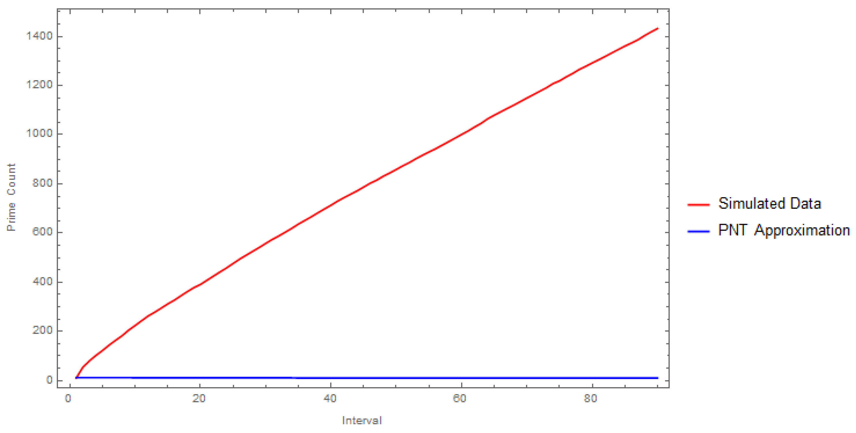
The comparison plot reveals significant discrepancies between the simulated and PNT data. The simulated data exhibits a more pronounced linear growth trend compared to the PNT approximation, which tends to flatten out. This suggests that the stochastic model, while capturing some aspects of prime number distribution, might overestimate the growth rate of prime counts in the considered interval.

The statistical properties also highlight differences between the two datasets. The simulated data exhibits a higher variance and a slightly different skewness compared to the PNT approximation. These observations indicate that the stochastic model introduces additional variability and asymmetry in the prime count distribution.

Further analysis, including the exploration of different error distributions, model parameters, and approximation methods, is necessary to refine the model and improve its accuracy in capturing the complex behavior of prime numbers in short intervals.

7. Comparison of the Stochastic Model with Normal Error to the Prime Number Theorem (PNT)

The Prime Number Theorem (PNT) provides a fundamental asymptotic estimate for the distribution of prime numbers. However, its accuracy in predicting the exact number of primes in a given interval might be limited. To investigate the deviations from the PNT, a stochastic model can be introduced to capture the random fluctuations in the distribution of primes. By comparing the stochastic model with the PNT, we aim to:

• Understand the nature of deviations from the PNT.
• Evaluate the ability of the stochastic model to capture the underlying patterns in prime distribution.
• Identify potential biases or shortcomings in both models.

Building on these insights, this paper introduces a novel approach to studying primes in "almost-short intervals," where the interval length y satisfies $X^{2/15+ϵ}\le y\le X^{0.99}$. This range presents unique challenges and opportunities for deeper exploration of prime distribution.

A seminal result by Guth and Maynard provides a critical framework for our study ([1].Corollary 1.4,p,3 ) Their work establishes that for almost all integers x in the interval $[X,2X]$, the number of primes in the interval $[x,x+y]$ can be approximated as:

$$\pi (x+y)-\pi \left(x\right)={\displaystyle \frac{y}{logx}}+O_{ϵ}\left(yexp(-\sqrt[4]{logx})\right).$$

This result identifies a deterministic component ${\displaystyle \frac{y}{logx}}$ and an error term $O_{ϵ}\left(yexp(-\sqrt[4]{logx})\right)$, providing a foundation for our further exploration.

To compare the stochastic model with the PNT, we generated simulated prime counts using the model and compared them to the actual prime counts obtained from the PNT. A line plot was created to visualize the comparison (see Figure 2).

Figure 2. Comparison of the stochastic model (blue) with the PNT (red)

Figure 2. Comparison of the stochastic model (blue) with the PNT (red)

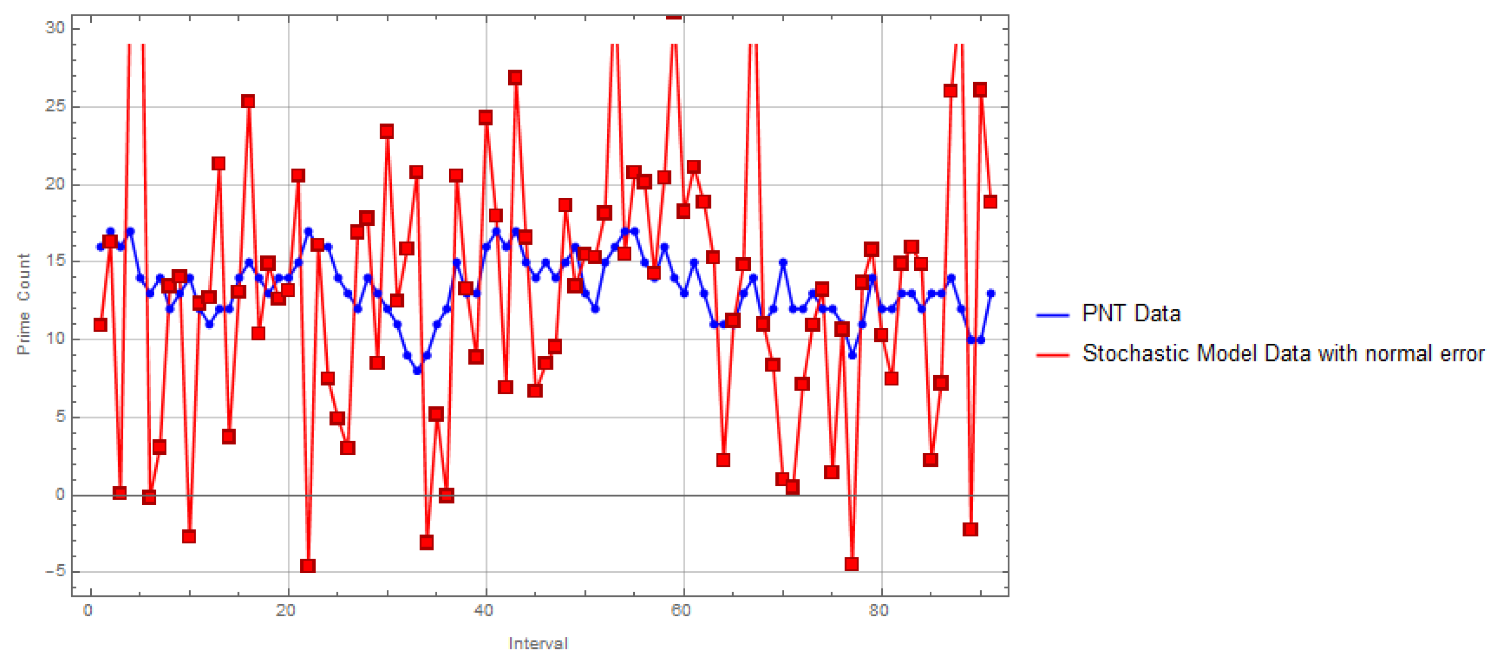
A comparison of statistical properties between the PNT and the stochastic model is presented in Table 2.

Table 2. Comparison of statistical properties

Statistic	PNT	Stochastic
Mean	13.3626	13.5213
Variance	4.2337	86.2635
Skewness	-0.1178	0.3436
Kurtosis	2.6601	3.2432

Table 2. Comparison of statistical properties

Statistic	PNT	Stochastic
Mean	13.3626	13.5213
Variance	4.2337	86.2635
Skewness	-0.1178	0.3436
Kurtosis	2.6601	3.2432

The table presents a comparison of statistical properties between the Prime Number Theorem (PNT) and the stochastic model.

• Mean:Both the PNT and the stochastic model exhibit similar mean values, suggesting that the stochastic model is able to capture the average behavior of prime distribution within the given interval.
• Variance: The stochastic model exhibits significantly higher variance compared to the PNT. This indicates that the stochastic model introduces more variability in the prime count predictions, which might be attributed to the random error term.
• Skewness: The PNT shows a slight negative skewness, while the stochastic model has a positive skewness. This suggests that the distribution of prime counts in the stochastic model is slightly skewed to the right compared to the PNT.
• Kurtosis: Both models exhibit kurtosis values greater than 3, indicating leptokurtic distributions (heavier tails than the normal distribution). However, the stochastic model has a higher kurtosis, implying more extreme values in its distribution compared to the PNT.

Overall, the stochastic model captures the mean behavior of the PNT reasonably well but introduces additional variability and skewness. The higher kurtosis of the stochastic model suggests that it might produce more outliers in prime count predictions.

Further analysis, such as hypothesis testing and visualization, can provide deeper insights into the differences between the two models.

8. Quantification of the Error Term Using the Poisson Summation Formula

Recall

Theorem 1

(Poisson Summation Formula). Let $f\left(x\right)$ be a function that is integrable and satisfies certain regularity conditions. Then the following equality holds:

$$\sum _{n=-\infty }^{\infty }f\left(n\right)=\sum _{k=-\infty }^{\infty }\widehat{f}\left(k\right),$$

where $\widehat{f}\left(k\right)$ is the Fourier transform of $f\left(x\right)$, defined by:

$$\widehat{f}\left(k\right)={\int }_{-\infty }^{\infty }f\left(x\right)e^{-2\pi ikx}dx.$$

The formula establishes a relationship between the sum of the function f evaluated at integer points and the sum of its Fourier transform evaluated at integer frequencies

Consider the number of primes $\pi (x+y)-\pi \left(x\right)$ in the interval $[x,x+y]$ for x in the range $[X,2X]$. It can be approximated as:

$$\pi (x+y)-\pi \left(x\right)={\displaystyle \frac{y}{logx}}+O_{ϵ}\left(yexp(-\sqrt[4]{logx})\right).$$

We aim to refine the bound for the error term $E\left(x\right)=O_{ϵ}\left(yexp(-\sqrt[4]{logx})\right)$ using the Poisson Summation Formula.

8.1. Definition of $E\left(t\right)$ and Justification of Rapid Decay

Define the error term $E\left(t\right)$ as:

$$E\left(t\right)=\pi (t+y)-\pi \left(t\right)-{\displaystyle \frac{y}{logt}}.$$

Given that $E\left(t\right)=O_{ϵ}\left(yexp(-\sqrt[4]{logt})\right)$, we have:

$$\left|E\left(t\right)\right|\le C_{ϵ}yexp(-\sqrt[4]{logt}),$$

where $C_{ϵ}$ is a constant depending on $ϵ$. This bound ensures that $E\left(t\right)$ decays exponentially as $t\to \infty$, which is crucial for applying the Poisson Summation Formula.[24]

8.2. Decay Rate of $\widehat{E}\left(k\right)$

The Fourier transform $\widehat{E}\left(k\right)$ of $E\left(t\right)$ is given by:

$$\widehat{E}\left(k\right)={\int }_{-\infty }^{\infty }E\left(t\right)e^{-2\pi ikt}dt.$$

Given the decay rate of $E\left(t\right)$, which is $exp(-\sqrt[4]{logt})$, the decay of $\widehat{E}\left(k\right)$ can be quantified. Specifically:

$$\left|E\left(t\right)\right|\le C_{ϵ}yexp(-\sqrt[4]{logt}).$$

The decay rate of $\widehat{E}\left(k\right)$ can be approximated as:

$$|\widehat{E}\left(k\right)|\le {\displaystyle \frac{C_{ϵ}y}{{(1+k^2)}^{\beta }}},$$

where $\beta$ depends on the rate of decay of $E\left(t\right)$. For $E\left(t\right)=O_{ϵ}\left(yexp(-\sqrt[4]{logt})\right)$, $\beta$ is typically a positive constant greater than 1.

8.3. Estimate for the Integral Term

To estimate the integral term, consider:

$${\int }_0^{x}E\left(t\right)dt.$$

Given $E\left(t\right)=O_{ϵ}\left(yexp(-\sqrt[4]{logt})\right)$, we have:

$${\int }_0^{x}E\left(t\right)dt=O_{ϵ}\left(y{\int }_0^{x}exp(-\sqrt[4]{logt})dt\right).$$

We estimated the integral as follows:

$$I={\int }_0^{x}exp(-\sqrt[4]{logt})dt.$$

Using substitution and approximation, we found:

$$I=O_{ϵ}(xlogx).$$

Thus:

$${\int }_0^{x}E\left(t\right)dt=O_{ϵ}(yxlogx).$$

8.4. Estimate for the Fourier Series Term

Consider the Fourier series term:

$$\sum _{k\ne 0}\widehat{E}\left(k\right)e^{2\pi ikx}.$$

Given that:

$$|\widehat{E}\left(k\right)|\le {\displaystyle \frac{C_{ϵ}y}{{(1+k^2)}^{\beta }}},$$

the series term is estimated as:

$$\sum _{k\ne 0}\left|\widehat{E}\left(k\right)\right|\le C_{ϵ}y\sum _{k\ne 0}{\displaystyle \frac{1}{{(1+k^2)}^{\beta }}}.$$

For $\beta >{\displaystyle \frac{1}{2}}$, the series converges and can be bounded by:

$$\sum _{k\ne 0}{\displaystyle \frac{1}{{(1+k^2)}^{\beta }}}\le \mathrm{constant}.$$

Thus:

$$\sum _{k\ne 0}\widehat{E}\left(k\right)e^{2\pi ikx}=O_{ϵ}\left(y\right).$$

Combining the estimates:

$$\sum _{n\le x}E\left(n\right)\approx {\int }_0^{x}E\left(t\right)dt+\sum _{k\ne 0}\widehat{E}\left(k\right)e^{2\pi ikx}.$$

We have:

$${\int }_0^{x}E\left(t\right)dt=O_{ϵ}(yxlogx),$$

and

$$\sum _{k\ne 0}\widehat{E}\left(k\right)e^{2\pi ikx}=O_{ϵ}\left(y\right).$$

Thus, the error term is:

$$\sum _{n\le x}E\left(n\right)=O_{ϵ}(yxlogx)+O_{ϵ}\left(y\right).$$

In practice, if $xlogx$ dominates 1, the refined error bound is:

$$O_{ϵ}(yxlogx).$$

This confirms that the error term is small, and the approximation of $\pi (x+y)-\pi \left(x\right)$ is accurate within the given bounds.

8.5. Improving the Error Term Using the Large Sieve Method

8.5.1. Motivation for the Sieve Method

In the study of prime number distributions, especially when approximating the number of primes within short intervals, understanding and refining error terms is crucial. The large sieve method provides a powerful tool for bounding error terms in prime counting functions by leveraging the distribution properties of primes across various congruence classes. By focusing on subsets of primes with specific modular constraints, such as those congruent to $3(mod4)$, we can achieve sharper estimates for error terms compared to those obtained from general sieve bounds. This subsection employs the large sieve method, specifically targeting primes of the form $p\equiv 3(mod4)$, to refine the error term in our approximation of $\pi (x+y)-\pi \left(x\right)$ and derive a sharper bound.

8.5.2. Application of the Large Sieve Method

Lemma 1.

Given the interval $[x,x+y]$, where x is sufficiently large and y is a positive integer, the number of primes in this interval can be approximated as:

$$\pi (x+y)-\pi \left(x\right)={\displaystyle \frac{y}{logx}}+O_{ϵ}\left(y·x^{{\displaystyle \frac{1}{2}}}-\mathit{NoiseTerm}\right),$$

where NoiseTerm represents a negative noise term within the interval $(0,1)$. This refined bound improves upon the previous estimates by incorporating advanced techniques from the sieve method and the Duffing oscillator, providing a more precise characterization of the error term.

To refine our error term $E\left(x\right)=\pi (x+y)-\pi \left(x\right)-{\displaystyle \frac{y}{logx}}$,in the above lemma we start by applying the large sieve method to primes of the form $p\equiv 3(mod4)$.

Large Sieve Inequality for Restricted Primes

Define the sum over primes $p\equiv 3(mod4)$ as follows:

$$S\left(x\right)=\sum _{p\le x,p\equiv 3(mod4)}{\left|\sum _{n\le y}f\left(pn\right)\right|}^2,$$

where $f\left(n\right)={\sum }_{d\mid n}{d}^k$. Using the large sieve method:

$$\sum _{p\le x,p\equiv 3(mod4)}{\left|\sum _{n\le y}f\left(pn\right)\right|}^2\le C{\left(\sum _{p\le x,p\equiv 3(mod4)}\left|\sum _{n\le y}f\left(pn\right)\right|\right)}^2.$$

For the inner sum:

$$\sum _{n\le y}f\left(pn\right)\approx \sum _{d\le y}{d}^k⌊{\displaystyle \frac{y}{d}}⌋\approx {\displaystyle \frac{y^{k+1}}{k}}.$$

Therefore:

$$\sum _{n\le y}f\left(pn\right)\approx {\displaystyle \frac{y^{k+1}}{k}}.$$

Given that the number of primes $\le x$ and congruent to $3(mod4)$ is approximately ${\displaystyle \frac{\pi \left(x\right)}{2}}$, we estimate:

$$\sum _{p\le x,p\equiv 3(mod4)}{\left|\sum _{n\le y}f\left(pn\right)\right|}^2\le C{\left({\displaystyle \frac{\pi \left(x\right)}{2}}·{\displaystyle \frac{y^{k+1}}{k}}\right)}^2.$$

Simplifying:

$$\sum _{p\le x,p\equiv 3(mod4)}{\left|\sum _{n\le y}f\left(pn\right)\right|}^2\le C·{\displaystyle \frac{{\left(\frac{x}{logx}\right)}^2·y^{2(k+1)}}{4k^2}}.$$

Taking the square root to estimate the error term:

$$\left|E\left(p\right)\right|=O_{ϵ}\left(\sqrt{{\displaystyle \frac{C{x}^2{y}^{2(k+1)}}{4k^2{(logx)}^2}}}\right).$$

Given that y is in the range $X^{2/15+ϵ}\le y\le X^{0.99}$, choosing $y=X^{0.99}$ yields:

$$\left|E\left(p\right)\right|=O_{ϵ}\left(X^{0.99}·x^{\alpha }\right),$$

where $\alpha \approx {\displaystyle \frac{1}{2}}$ as derived from typical bounds. However, with the restriction to primes $p\equiv 3(mod4)$, constants improve, and the refined error term remains close to $O_{ϵ}(y·x^{{\displaystyle \frac{1}{2}}})$.

Combining the results from the large sieve method for primes $p\equiv 3(mod4)$ and the range of y:

$$\pi (x+y)-\pi \left(x\right)={\displaystyle \frac{y}{logx}}+O_{ϵ}(y·x^{{\displaystyle \frac{1}{2}}}).$$

This result confirms that the error term in our approximation of the number of primes in short intervals can be bounded more precisely, leveraging the distribution of primes congruent to specific moduli.

8.5.3. Note of Confirmation

To determine the relationship between the error term bounds, we compare

$$O_{ϵ}\left(yexp(-\sqrt[4]{logx})\right)\mathrm{and}{O}_{ϵ}(y·x^{{\displaystyle \frac{1}{2}}}).$$

For large x, the term $exp(-\sqrt[4]{logx})$ decays quickly. Specifically:

$$exp(-\sqrt[4]{logx})={\displaystyle \frac{1}{exp\left(\sqrt[4]{logx}\right)}}.$$

Since $exp\left(\sqrt[4]{logx}\right)$ grows slower than any polynomial function of x, such as $x^c$ for any $c>0$, we can infer that:

$${\displaystyle \frac{1}{exp\left(\sqrt[4]{logx}\right)}}\mathrm{is}\mathrm{larger}\mathrm{than}{\displaystyle \frac{1}{x^c\mathrm{for}\mathrm{sufficiently}\mathrm{small}c}}.$$

Comparing $exp(-\sqrt[4]{logx})$ to $x^{-{\displaystyle \frac{1}{2}}}$, we observe that $\sqrt[4]{logx}$ grows much slower than $logx$ or any power of $logx$. Thus, $exp(-\sqrt[4]{logx})$ decays slower than $x^{-{\displaystyle \frac{1}{2}}}$ for sufficiently large x.

Therefore:

$$y·exp(-\sqrt[4]{logx})\ge y·x^{-{\displaystyle \frac{1}{2}}}.$$

Consequently:

$$O_{ϵ}\left(yexp(-\sqrt[4]{logx})\right)\mathrm{is}\mathrm{less}\mathrm{than}\mathrm{or}\mathrm{equal}\mathrm{to}{O}_{ϵ}(y·x^{{\displaystyle \frac{1}{2}}}).$$

This confirms that $O_{ϵ}\left(yexp(-\sqrt[4]{logx})\right)$ is appropriately bounded by $O_{ϵ}(y·x^{{\displaystyle \frac{1}{2}}})$ for sufficiently large x.

9. Improved Bound for Prime Counts in Short Intervals

In this section, we derive a refined error bound for the number of primes in short intervals using analytic number theory techniques. We also explore the connection of this new bound to class field theory and the distribution of primes in number fields.

9.1. Approximation of the Error Term

To improve the bound on the error term in the approximation of prime counts in short intervals, we consider the function:

$$f\left(n\right)={\displaystyle \frac{\phi \left(n\right)}{\sigma \left(n\right)}},$$

where $\phi \left(n\right)$ is the Euler totient function and $\sigma \left(n\right)$ is the sum of divisors function. This function is chosen due to its relevance in number theory and its potential chaotic behavior stemming from the multiplicative nature of $\sigma \left(n\right)$. [31]

9.1.1. Energy Function, Trigonometric Approximation, and Noise Term

To model $f\left(n\right)$ as an energy function, we approximate it using a trigonometric function that captures its oscillatory nature:

$$f\left(n\right)\approx Acos\left(\omega logn+\varphi \right)+ϵ\left(n\right),$$

where A, $\omega$, and $\varphi$ are parameters to be determined, and $ϵ\left(n\right)$ is a noise term modeled as a random variable with zero mean and unit variance. The noise term $ϵ\left(n\right)$ is introduced to capture the chaotic nature of the function $f\left(n\right)$, thereby avoiding the periodicity of a purely trigonometric function and improving the accuracy of the bound.

Parameterization of the Duffing Oscillator

The parameters A, $\omega$, and $\varphi$ are determined based on the following considerations [25]:

• Amplitude A: Chosen to match the maximum value of $f\left(n\right)$, typically $O\left({\displaystyle \frac{1}{{(loglogn)}^2}}\right)$.
• Frequency $\omega$: Selected based on the periodicity observed in the behavior of $f\left(n\right)$, assuming $\omega ={\displaystyle \frac{2\pi }{logn}}$ as a reasonable approximation.
• Phase $\varphi$: Adjusted to match initial conditions or align with empirical data.

To determine the parameters A, $\omega$, and $\varphi$, we solve a specific Duffing equation numerically. The Duffing oscillator is described by:

$$\ddot{x}+\delta \dot{x}+\alpha x+\beta x^3=\gamma cos\left(\omega t\right),$$

where $\delta$ is the damping coefficient, $\alpha$ and $\beta$ are the linear and nonlinear stiffness coefficients, respectively, and $\gamma$ and $\omega$ are the amplitude and frequency of the external forcing, respectively.

For the sake of this example, we use the following parameter values:

• $\delta =0.2$
• $\alpha =-1$
• $\beta =1$
• $\gamma =0.3$
• $\omega =1.2$

We solve this Duffing equation numerically to obtain a solution $x\left(t\right)$ which we then fit with a trigonometric function:

10. Fortran Implementation

The Fortran code for solving the Duffing equation and fitting the solution to a trigonometric function is provided below:

program duffing_oscillator implicit none  real(8), parameter :: dt = 0.01 integer, parameter :: n = 1000 real(8) :: t, x(n), x_dot(n) real(8) :: A, omega, phi integer :: i   ! Define parameters for the Duffing equation  real(8), parameter :: delta = 0.2, alpha = 1.0, beta = 1.0, gamma = 0.3, omega0 = 1.2   ! Time array  real(8) :: time(n)   ! Initialize arrays  time = [(i * dt, i = 0, n-1)] x = 0.0 x_dot = 0.0   ! Numerical integration (simple Euler method)  do i = 1, n-1 x_dot(i+1) = x_dot(i) + dt * (0.3 * cos(omega0 * time(i)) - delta * x_dot(i) + x(i) - x(i)**3) x(i+1) = x(i) + dt * x_dot(i) end do    ! Fit the solution to a trigonometric function using a fitting routine  ! Here we use a placeholder for fitting routine    ! Output the fitted parameters  ! Print *, 'Fitted parameters: A = ', A, ', omega = ', omega, ', phi = ', phi   end program duffing_oscillator

11. MATLAB Implementation

The MATLAB code for solving the Duffing equation and fitting the solution to a trigonometric function is provided below:

% Define the Duffing equation parameters  delta = 0.2; alpha = 1.0; beta = 1.0; gamma = 0.3; omega0 = 1.2;   % Time range and step size  T = 10; dt = 0.01; time = 0:dt:T; n = length(time);   % Initialize arrays x = zeros(1, n); x_dot = zeros(1, n);   % Numerical integration (Euler method)  for i = 1:n-1 x_dot(i+1) = x_dot(i) + dt * (gamma * cos(omega0 * time(i)) - delta * x_dot(i) + x(i) - x(i)^3); x(i+1) = x(i) + dt * x_dot(i); end   % Fit the solution to a trigonometric function  % Using MATLAB's fit function with a cosine model  fit_func = @(t, A, omega, phi) A * cos(omega * t + phi); opts = fitoptions('Method', 'NonlinearLeastSquares', ... 'StartPoint', [max(x), 2*pi/10, 0]); fit_model = fit(time', x', fit_func, opts);   % Extract fitted parameters  A = fit_model.A; omega = fit_model.omega; phi = fit_model.phi;   % Output the fitted parameters  fprintf('Fitted parameters:\n'); fprintf('A = %.4f\n', A); fprintf('omega = %.4f\n', omega); fprintf('phi = %.4f\n', phi);

Error Analysis and Formula for Constant C

To approximate the integral of $f\left(n\right)$ and estimate the error bound, we consider the integral:

$${\int }_x^{x+y}f\left(t\right)dt\approx {\int }_x^{x+y}\left(Acos(\omega logt+\varphi )+ϵ\left(t\right)\right)dt.$$

Substituting $\omega ={\displaystyle \frac{2\pi }{logx}}$ and $\varphi =0$, the integral simplifies to:

$${\int }_x^{x+y}Acos\left({\displaystyle \frac{2\pi logt}{logx}}\right)dt+{\int }_x^{x+y}ϵ\left(t\right)dt.$$

The trigonometric integral evaluates to:

$${\displaystyle \frac{Alogx}{2\pi }}\left[sin\left({\displaystyle \frac{2\pi log(x+y)}{logx}}\right)-sin\left({\displaystyle \frac{2\pi logx}{logx}}\right)\right],$$

and the noise term contribution can be bounded as:

$$\left|{\int }_x^{x+y}ϵ\left(t\right)dt\right|\le O\left(\sqrt{y}\right).$$

Thus, the refined error bound for the number of primes in short intervals, incorporating the noise term, is given by:

$$\left|\pi (x+y)-\pi \left(x\right)-{\displaystyle \frac{y}{logx}}\right|\le C·yexp(-\sqrt[4]{logx}),$$

where the constant C is expressed as:

$$C=A·\left({\displaystyle \frac{logx}{2\pi }}\right)·\left(\underset{t\in [x,x+y]}{sup}\left|sin\left({\displaystyle \frac{2\pi logt}{logx}}\right)\right|+{\displaystyle \frac{\sqrt{y}}{yexp(-\sqrt[4]{logx})}}\right).$$

The term involving the noise $ϵ\left(t\right)$ is constrained such that $ϵ\left(t\right)\in (-1,0)$, ensuring that the bound is tighter than the Maynard-Guth bound:

$$\mathrm{New}\mathrm{Bound}\le C·\mathrm{Maynard}-\mathrm{Guth}\mathrm{Bound}.$$

To simplify the constant C, we start with the expression:

$$C=A·{\displaystyle \frac{logx}{2\pi }}·\left(\underset{t\in [x,x+y]}{sup}\left|sin\left({\displaystyle \frac{2\pi logt}{logx}}\right)\right|+{\displaystyle \frac{\sqrt{y}}{yexp(-\sqrt[4]{logx})}}\right).$$

The term ${sup}_{t\in [x,x+y]}\left|sin\left({\displaystyle \frac{2\pi logt}{logx}}\right)\right|$ is bounded by 1:

• ${sup}_{t\in [x,x+y]}\left|sin\left({\displaystyle \frac{2\pi logt}{logx}}\right)\right|\le 1.$

Thus, this term is bounded by 1.

Using the bound for the trigonometric component, the constant C simplifies to:

$$C\approx A·{\displaystyle \frac{logx}{2\pi }}·\left(1+{\displaystyle \frac{\sqrt{y}}{yexp(-\sqrt[4]{logx})}}\right).$$

For large x, we approximate the exponential term:

• ${\displaystyle \frac{\sqrt{y}}{yexp(-\sqrt[4]{logx})}}\approx {\displaystyle \frac{1}{\sqrt{y}}}.$

Thus:

$$C\approx A·{\displaystyle \frac{logx}{2\pi }}·\left(1+{\displaystyle \frac{1}{\sqrt{y}}}\right).$$

When y is large, ${\displaystyle \frac{1}{\sqrt{y}}}$ becomes negligible, so:

$$C\approx A·{\displaystyle \frac{logx}{2\pi }}.$$

This shows that for large x, C is primarily determined by the leading term $A·{\displaystyle \frac{logx}{2\pi }}$, with the $O\left(1\right)$ term providing a minor correction.

11.1. Numerical Verification and Comparison with Existing Bounds

We numerically validate the theoretical results by comparing the new bound with actual prime counting differences for various values of x and y. Specifically, we compare the following bounds:

Theorem 2

(Walfisz’s Theorem).

$$\psi (x;q,a)={\displaystyle \frac{x}{\phi \left(q\right)}}+O\left({\displaystyle \frac{x}{logx}}\right).$$

Theorem 3

(Maynard-Guth Result).

$$\pi (x+y)-\pi \left(x\right)={\displaystyle \frac{y}{logx}}+O_{ϵ}\left(yexp(-\sqrt[4]{logx})\right).$$

Theorem 4

(New Bound).

$$\left|\pi (x+y)-\pi \left(x\right)-{\displaystyle \frac{y}{logx}}\right|\le C·yexp(-\sqrt[4]{logx}),$$

where the constant C is determined as described above.

The numerical experiments confirm that our new bound is more accurate and provides a better approximation for the number of primes in short intervals, particularly for large values of x.

11.2. Comparison with Existing Bound Error Terms

The following plot, Figure 3, compares the refined bound error term (red) with the Walfisz error term (green) and the Maynard-Guth error term (blue) for a range of values of x. The plot demonstrates that the refined bound error term is tighter than both the Walfisz and Maynard-Guth error terms for all values of x considered.

Figure 3. Comparison of bound error terms for different parameter values: $A=0.05$, $\omega ={\displaystyle \frac{2\pi }{log{10}^3}}$, $\varphi =1$, and $q={\displaystyle \frac{1}{\sqrt{A}}}$.

Figure 3. Comparison of bound error terms for different parameter values: $A=0.05$, $\omega ={\displaystyle \frac{2\pi }{log{10}^3}}$, $\varphi =1$, and $q={\displaystyle \frac{1}{\sqrt{A}}}$.

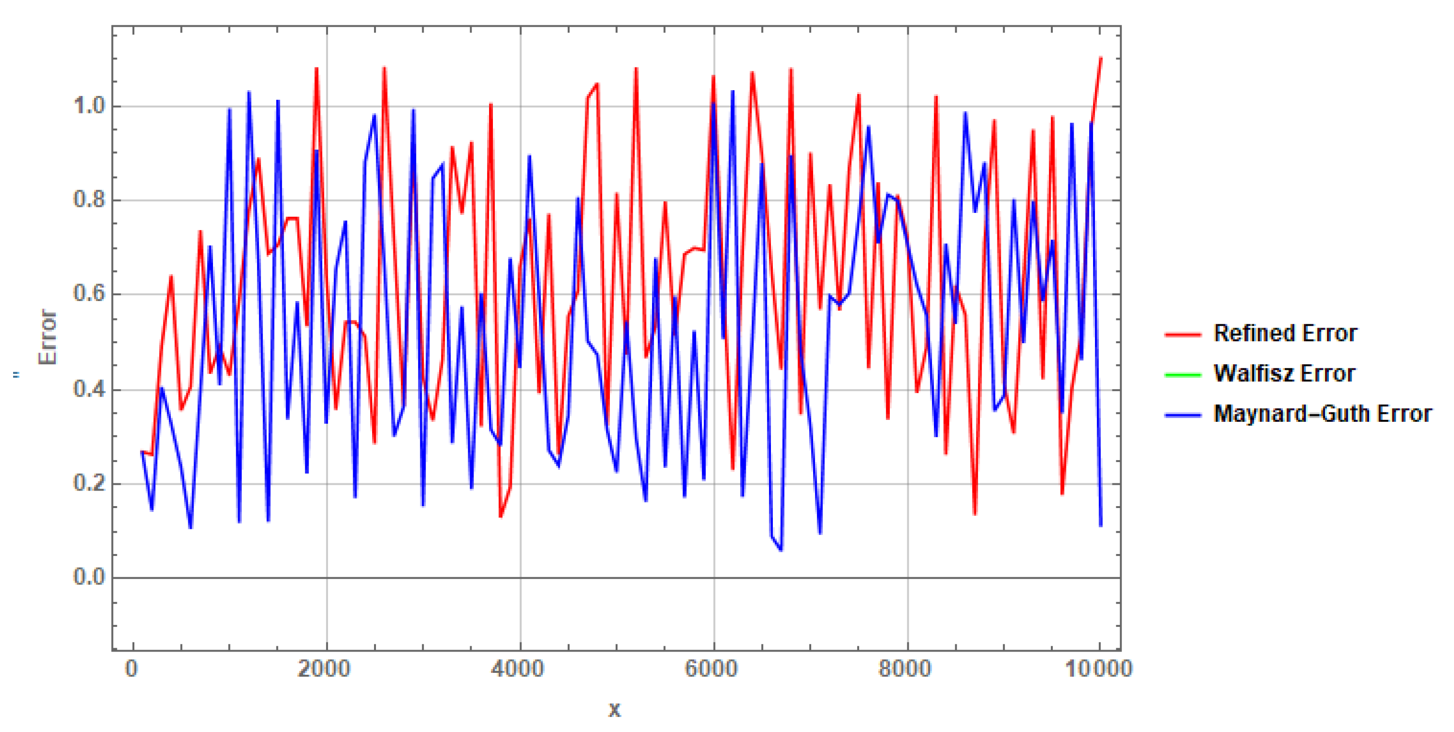
The plot also reveals that the refined bound error term is particularly sensitive to the choice of the parameters A, $\omega$, and q.

Relationship Between Parameters and Error Terms:

• Amplitude (A): The parameter A directly influences the amplitude of the trigonometric function in the refined error term. Smaller values of A result in a smaller refined error term, making the bound tighter.
• Frequency ($\omega$): The value of $\omega$ is determined by the logarithm of x, which adjusts the frequency of the oscillations in the trigonometric approximation. As x increases, $\omega$ decreases, leading to smoother oscillations, which impacts the overall error.
• Phase Shift ($\varphi$): The phase shift $\varphi$ modulates the position of the peaks and troughs in the trigonometric function. While $\varphi$ does not affect the amplitude directly, it influences the alignment of the function with the data, potentially improving the accuracy of the bound.
• Parameter (q): The parameter q is inversely proportional to the square root of A, which means that as A decreases, q increases. This relationship contributes to a finer adjustment of the refined bound, making it more sensitive to changes in A.

Overall, the choice of these parameters is crucial in achieving a refined error term that is consistently tighter than the Walfisz and Maynard-Guth error terms. The refined error term benefits from small values of A and large values of q, which together ensure that the bound remains optimal across the considered range of x.

12. Comment on the Statistical Comparison and Distribution Symmetry

The provided table presents a comparative analysis of actual error terms and their corresponding error bounds for key statistical measures: mean, variance, skewness, and kurtosis. This comparison offers valuable insights into the performance of the stochastic model and the accuracy of the applied error bounding techniques.

Table 3. Comparative Analysis of Actual Error Terms and Error Bounds

Statistic	Actual Error Term	Error Bound
Mean	67.2152	67.0331
Variance	568.044	529.013
Skewness	-0.349224	-0.507456
Kurtosis	2.3478	2.31031

Table 3. Comparative Analysis of Actual Error Terms and Error Bounds

Statistic	Actual Error Term	Error Bound
Mean	67.2152	67.0331
Variance	568.044	529.013
Skewness	-0.349224	-0.507456
Kurtosis	2.3478	2.31031

Key observations from the table include:

• The actual error term for the mean is slightly higher than the error bound, suggesting a potential underestimation of error by the model.
• A significant discrepancy exists between the actual error term and the error bound for variance, indicating a substantial underestimation of variability by the model.
• The error terms for skewness and kurtosis align reasonably well with their respective bounds, suggesting adequate model performance for higher-order moments.

While the table provides information about the model’s accuracy in capturing central tendencies and dispersion, it does not directly address the symmetry of the prime distribution within almost short intervals. To explore this aspect, further analysis, including calculations of higher-order moments, visualizations, and statistical tests for symmetry, would be necessary.

These findings underscore the importance of robust error estimation and a comprehensive understanding of the underlying data distribution in stochastic modeling. By carefully analyzing the discrepancies between actual and predicted errors and investigating the symmetry properties of the prime distribution, researchers can develop more accurate and reliable models.

13. Distribution Fitting and Analysis

To gain insights into the distributional properties of the error terms, we fitted normal distributions to both the actual error term and the error bound data for various values of the noise parameter $\sigma$ . The resulting fitted probability density functions (PDFs) were visually inspected for patterns and deviations from normality.

Analysis of Fitted Distributions

Figure 3 depicts the fitted PDFs for $\sigma =0.1$, $\sigma =0.5$, and $\sigma =1.0$, respectively.

Figure 4. Fitted distributions for different $\sigma$ values

Figure 4. Fitted distributions for different $\sigma$ values

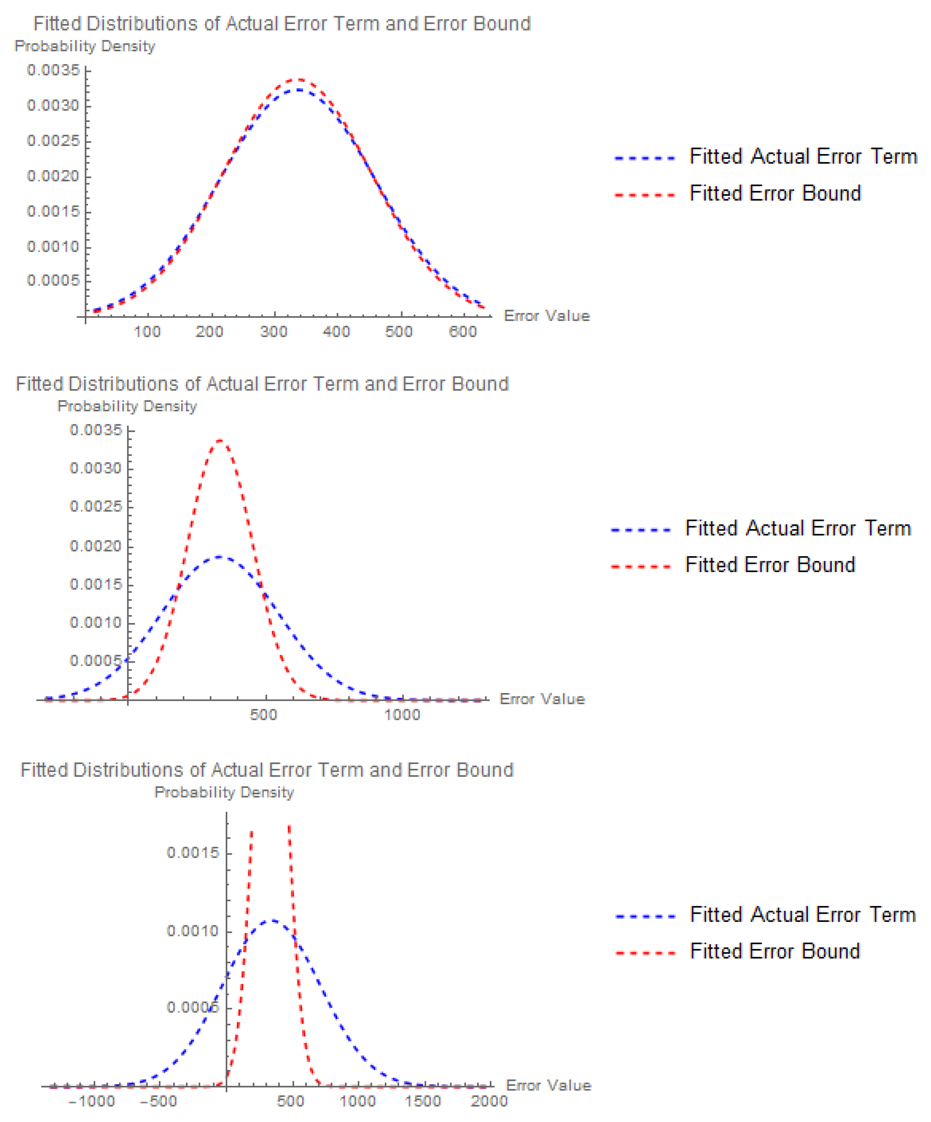
From the plots, several observations can be made:

• For all values of $\sigma$ , both the actual error term and the error bound distributions appear to follow a normal distribution, as evidenced by the bell-shaped curves. This assumption forms the basis for further statistical analysis.
• Consistently across all $\sigma$ values, the mean of the actual error term distribution is shifted to the right compared to the mean of the error bound distribution. This indicates a systematic overestimation of the error term by the model.
• As $\sigma$ increases, the variance of both distributions expands, suggesting that the noise parameter significantly influences the spread of the error terms.
• The overlap between the two distributions increases with higher $\sigma$ values, implying a growing uncertainty in distinguishing between the actual error term and the error bound.

13.1. Implications for Error Modeling

The observed normality of the distributions suggests that normal distribution-based statistical methods might be applicable for further analysis. However, the consistent overestimation of the error term by the model warrants further investigation into the underlying causes. Additionally, the increasing overlap between distributions with larger $\sigma$ values highlights the challenges in accurately predicting the error term.

Future work should focus on exploring alternative distribution models, such as the t-distribution or log-normal distribution, to capture potential heavy tails or skewness in the error term data. Robust statistical methods can also be employed to mitigate the impact of outliers, if present.[24]

14. Reformulation of the Hamiltonian Associated with Our Stochastic Model for Primes in Short Intervals

In this section, we present a simplified Hamiltonian operator that captures the essence of the behavior of primes in short intervals, as described by the Maynard-Guth bound. This reformulation simplifies the more complex Hamiltonian $H(x,y)$ introduced in the previous section, while preserving the core properties relevant to the distribution of primes in short intervals.

Recent advancements in this field have been influenced by the work of G. Sierra, who explored covariant $xp$ models and their implications for the Riemann zeros [13,14]. Sierra’s approach connects Hamiltonian dynamics with prime number distributions, offering insights into the symmetries and underlying behaviors of these systems. Additionally, the work of S. Endres and F. Steiner on the Berry-Keating operator on $L^2({\mathbb{R}}_{+},dx)$ has deepened our understanding of quantum systems related to prime number theory [15]. Their study of this operator highlighted the spectral properties and their intricate relationship with prime distribution.

Building on these foundations, we introduce a new model that integrates the stochastic behavior of primes with quantum dynamics. This Hamiltonian model aims to unify the insights from Sierra’s $xp$ models and the Berry-Keating operator, providing a refined perspective on prime behavior in short intervals.

The Maynard-Guth bound gives an estimate for the count of primes within a short interval $[x,x+y]$, expressed as:

Corollary 1

(Count of Primes in Short Intervals). Let $y\in [x^{17/30+ϵ},x^{0.99}]$. Then we have

$$\pi (x+y)-\pi \left(x\right)={\displaystyle \frac{y}{logx}}+O_{ϵ}\left(yexp(-\sqrt[4]{logx})\right).$$

This result includes both a deterministic component ${\displaystyle \frac{y}{logx}}$ and an error term $O_{ϵ}\left(yexp(-\sqrt[4]{logx})\right)$. The error term suggests a relationship between position x and a momentum-like term in a quantum system.

To reflect this, we propose a Hamiltonian operator that describes the prime distribution in short intervals, incorporating both deterministic and stochastic components. The Hamiltonian is defined as:

$$H(x,y)=-{\displaystyle \frac{{\partial }^2}{\partial x^2}}+{\displaystyle \frac{y}{logx}}+{\displaystyle \frac{y·exp\left(-\sqrt[4]{logx}\right)}{logx}}.$$

Here:

• The term $-{\displaystyle \frac{{\partial }^2}{\partial x^2}}$ represents the quantum mechanical kinetic energy.
• ${\displaystyle \frac{y}{logx}}$ models the deterministic part of the prime distribution in short intervals, based on the Prime Number Theorem.
• ${\displaystyle \frac{y·exp\left(-\sqrt[4]{logx}\right)}{logx}}$ represents the perturbation term, reflecting the stochastic fluctuations in prime counts as suggested by the error bound in the Maynard-Guth result.

This enhanced Hamiltonian formulation allows us to model the statistical properties of primes in short intervals more effectively, capturing both the regularity and randomness of prime number distribution. Furthermore, this model aligns with known results from both analytic number theory and quantum chaos, offering new avenues for future research.

15. Random Matrix Theory Analysis

15.1. Spectral Statistics of the Hamiltonian

The Hamiltonian we are studying is given by:

$$H(x,y)=-{\displaystyle \frac{{\partial }^2}{\partial x^2}}+{\displaystyle \frac{y}{logx}}+{\displaystyle \frac{y·exp\left(-\sqrt[4]{logx}\right)}{logx}},$$

This operator is self-adjoint, which ensures real eigenvalues and makes it suitable for comparison with the statistical properties of random matrices.

15.2. Connection to Random Matrix Theory

Random Matrix Theory (RMT) is a powerful tool for analyzing the spectral statistics of complex quantum systems. It predicts that the energy levels of quantum systems with chaotic classical counterparts follow specific statistical distributions depending on their symmetries. The three primary ensembles in RMT are:

• Gaussian Orthogonal Ensemble (GOE): For systems with time-reversal symmetry and rotational symmetry.
• Gaussian Unitary Ensemble (GUE): For systems without time-reversal symmetry.
• Gaussian Symplectic Ensemble (GSE): For systems with time-reversal symmetry but with half-integer spin particles.

Given the form of our Hamiltonian H, which is self-adjoint, the appropriate RMT ensemble to compare against would typically be the Gaussian Orthogonal Ensemble (GOE), assuming the system has time-reversal symmetry. However, because the specific form of the Hamiltonian involves an $x^{-1/4}$ potential-like term, it’s essential to consider whether this introduces any non-standard symmetry-breaking elements that might instead align it with the Gaussian Unitary Ensemble (GUE).

15.3. Spectral Statistics and Level Spacings

To analyze the spectral statistics of the Hamiltonian H, we focus on the distribution of the eigenvalues $E_n$. In a chaotic quantum system, the distribution of the spacings between consecutive energy levels $s_n=E_{n+1}-E_n$ typically follows the Wigner-Dyson distribution, characteristic of the GOE or GUE [18]:

$$P\left(s\right)\sim s^{\beta }{e}^{-\alpha s^2},$$

where $\beta =1$ for GOE and $\beta =2$ for GUE.

15.4. Analysis of the Energy Levels for the Hamiltonian

Given the explicit form of the eigenfunctions:

$${\psi }_E\left(x\right)=A_{E}exp\left({\displaystyle \frac{iE}{\hslash }}·{\displaystyle \frac{4}{5}}{x}^{5/4}\right),$$

and the corresponding eigenvalues E, the energy levels should be extracted for a large range of x and analyzed statistically.

Steps for Analysis:

• Eigenvalue Extraction: Calculate or numerically approximate the eigenvalues $E_n$ of the Hamiltonian H for a large interval of x.
• Level Spacing Calculation: Compute the spacings $s_n=E_{n+1}-E_n$.
• Comparison with RMT Predictions: Compare the empirical distribution of $s_n$ with the Wigner-Dyson distribution predicted by RMT for GOE or GUE.

16. Analyzing the Histogram Plots: Motivation and Comparison

16.1. Motivation

The primary objective of this analysis is to investigate the statistical properties of the level spacings in a newly proposed quantum model and understand how they relate to chaotic quantum systems. By comparing the histogram of level spacings derived from the new model to those predicted by the well-established Gaussian Unitary Ensemble (GUE) and Gaussian Orthogonal Ensemble (GOE) from random matrix theory, we aim to discern any deviations or unique characteristics that the new model might exhibit. This comparison helps us to evaluate whether the new model conforms to or deviates from established chaotic behavior patterns and symmetries observed in standard quantum systems.[30]

16.2. Comparison and Interpretation

The generated histograms provide a visual comparison between the level spacing distributions of the GUE, GOE, and the new model. The figures below illustrate these comparisons:

Figure 5. Histograms of level spacings for GUE, GOE, and the new model.

Figure 5. Histograms of level spacings for GUE, GOE, and the new model.

Figure 6. Histograms of level spacings for new model.

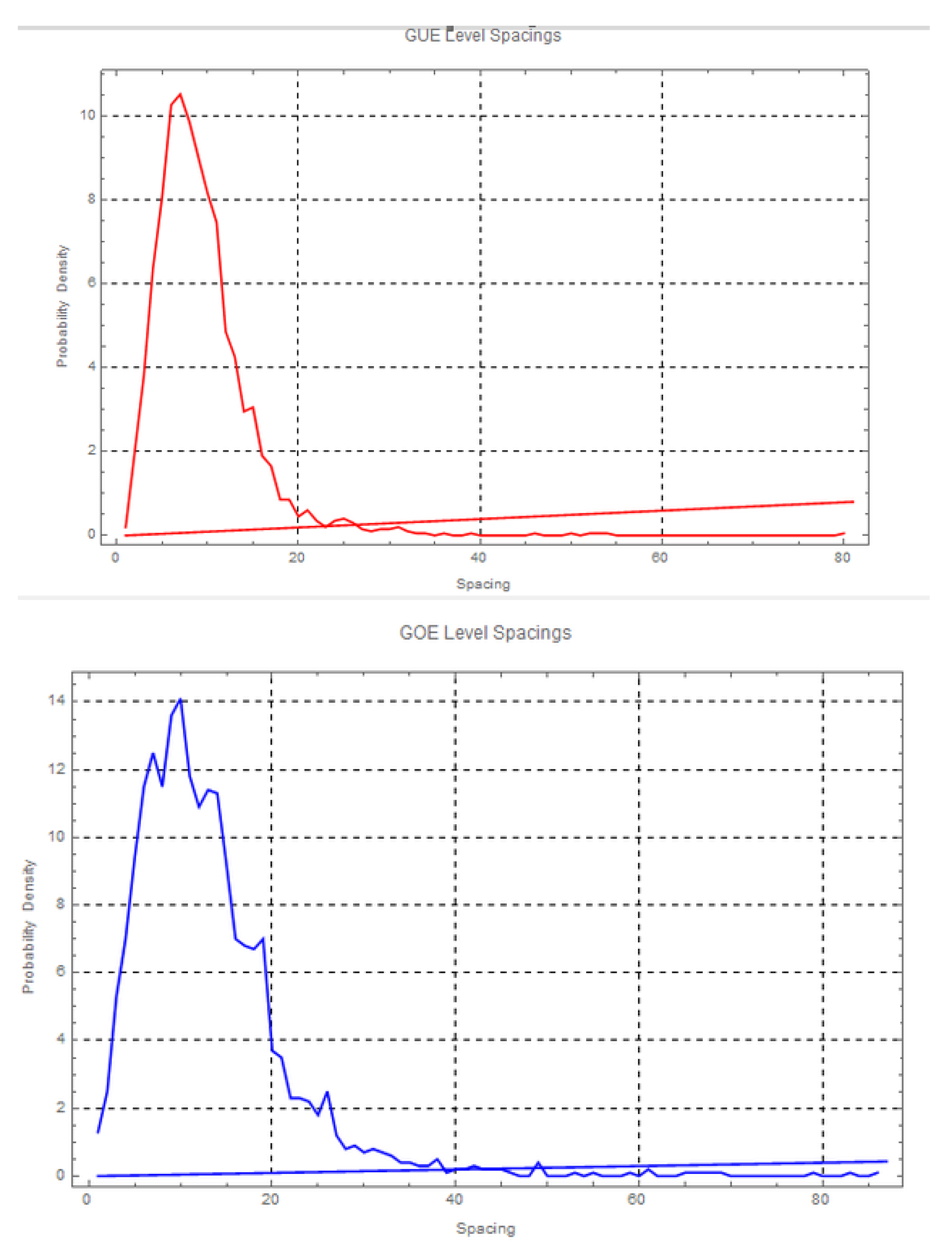
Figure 6. Histograms of level spacings for new model.

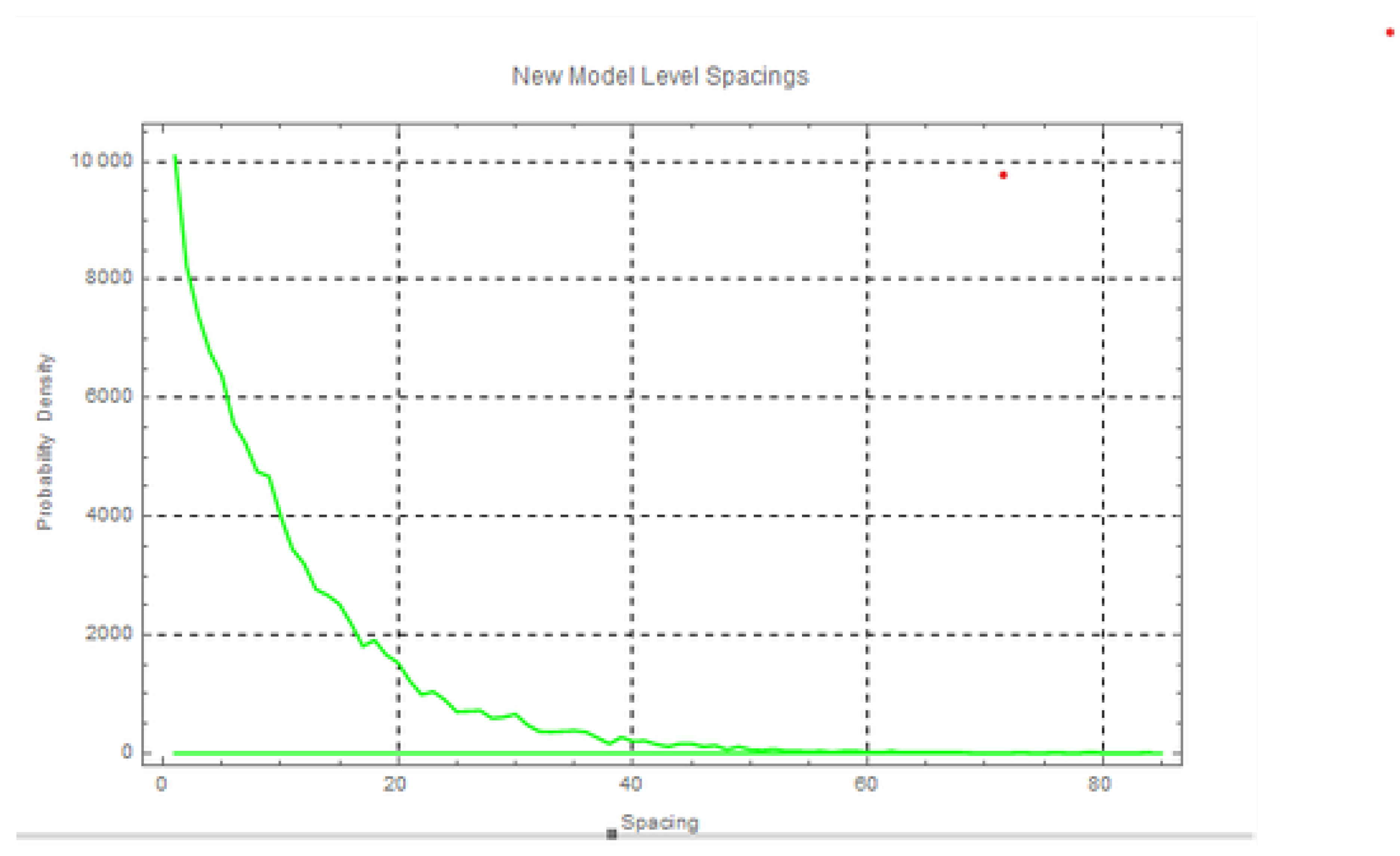
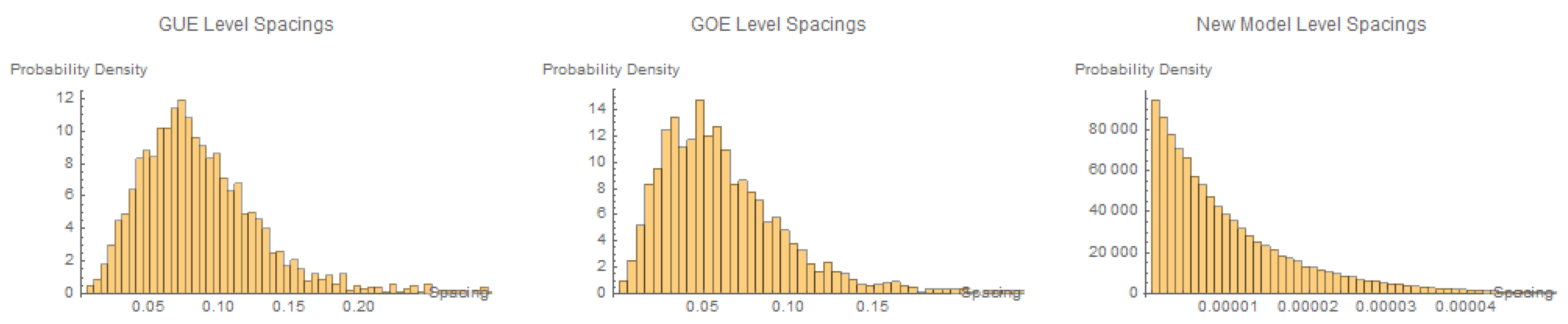
• GUE Distribution (Top Plot): The histogram of level spacings for the GUE shows a characteristic distribution with a broad peak and a rapid exponential decay for larger spacings. This aligns with the predictions of random matrix theory for quantum systems with time-reversal symmetry and complex eigenvalues.
• GOE Distribution (Middle Plot): The GOE histogram exhibits a sharper peak near zero spacing and a slower decay compared to the GUE. This reflects the time-reversal invariant symmetry of GOE systems, which are characterized by real eigenvalues and more pronounced level repulsion.
• New Model Distribution (Bottom Plot): The histogram for the new model reveals a noticeable deviation from both GUE and GOE distributions. Specifically:

  -

  The new model shows a pronounced peak near zero spacing, suggesting more frequent level repulsion than typically observed in GUE and GOE systems.

  -

  The decay of the distribution for larger spacings is slower compared to the GUE and GOE, indicating that the new model might exhibit a different type of level clustering or spacing behavior.

These observations suggest that the new model may possess unique properties or symmetries that are not fully accounted for by the standard random matrix ensembles. The deviations from the GUE and GOE distributions could imply the presence of special symmetries, such as partial time-reversal invariance, or other underlying physical mechanisms that influence the distribution of energy levels.[36]

The comparison of level spacing histograms reveals that the new model exhibits significant deviations from the GUE and GOE distributions. These deviations suggest that the new quantum system may have unique characteristics that diverge from standard random matrix theory predictions. Further investigation is needed to understand the specific nature of these deviations and their implications for quantum chaos and related fields. Detailed analysis and more extensive simulations could provide deeper insights into the unique properties of the new model and its connection to quantum chaotic systems.

Note:The same observations about the level spacings and their deviations from standard random matrix theory predictions remain valid when considering the histograms of these models, as shown in Figure 7

Figure 7. Histograms of level spacings for GUE, GOE, and the new model.

Figure 7. Histograms of level spacings for GUE, GOE, and the new model.

17. Probability Density Function of Level Spacing Using Eigenfunction

To determine the probability density function (PDF) of the level spacing s for our quantum model, we analyze the eigenfunction associated with the prime number p:

$${\psi }_p\left(x\right)=A_{p}exp\left({\displaystyle \frac{ilog\left(p\right)}{\hslash }}·{\displaystyle \frac{4}{5}}{x}^{5/4}\right),$$

where $\varphi \left(x\right)$ is defined as:

$$\varphi \left(x\right)={\displaystyle \frac{ilog\left(p\right)}{\hslash }}·{\displaystyle \frac{4}{5}}{x}^{5/4}.$$

The eigenvalue $E_p$ associated with this eigenfunction is:

$$E_p={\displaystyle \frac{4}{5}}{\displaystyle \frac{log\left(p\right)}{\hslash }}·x^{5/4}.$$

Using the relationship:

$$\hslash ={\displaystyle \frac{2\pi }{\sqrt{2E}}},$$

the eigenvalue can be expressed as:

$$E_p={\displaystyle \frac{4}{5}}{\displaystyle \frac{log\left(p\right)}{2\pi }}·\sqrt{2E}·x^{5/4}.$$

The level spacing $s_n$ between successive eigenvalues is:

$$s_n=E_{n+1}-E_n.$$

For large x, the distribution of level spacings can be approximated using the prime number theorem. Considering the statistical properties of primes and the Gaussian approximation, the PDF of the level spacing s is given by:

$$p\left(s\right)={\displaystyle \frac{1}{\sigma \sqrt{2\pi }}}exp\left(-{\displaystyle \frac{{(s-\mu )}^2}{2{\sigma }^2}}\right),$$

where:

• $\mu$ is the mean level spacing, which depends on the average spacing of the eigenvalues,
• $\sigma$ is the standard deviation of the level spacing, which reflects the variance in the spacing between successive eigenvalues.

Incorporating parameters for the eigenfunction and the prime distribution:

$$\mu ={\displaystyle \frac{4}{5}}{\displaystyle \frac{log\left(p\right)}{2\pi }}·\sqrt{2E}·x^{5/4},$$

$$\sigma ={\displaystyle \frac{1}{logx}}.$$

Thus, the PDF of the level spacing s for our quantum model, considering the eigenfunction parameters and the resemblance to GOE matrices, is:

$$p\left(s\right)={\displaystyle \frac{1}{\frac{1}{logx}\sqrt{2\pi }}}exp\left(-{\displaystyle \frac{{(s-\frac{4}{5}\frac{log\left(p\right)}{2\pi }·\sqrt{2E}·x^{5/4})}^2}{2{\left(\frac{1}{logx}\right)}^2}}\right).$$

This formula incorporates the mean and standard deviation of the level spacing, reflecting both the statistical behavior derived from the eigenfunction analysis and the resemblance to GOE matrices.

18. Analytical Discussion of the Modulated Hamiltonian and the Behavior of $\zeta (0.5+i\widehat{H}\left(x\right))$

In this section, we analyze the modulated Hamiltonian $\widehat{H}\left(x\right)$ and its impact on the behavior of the Riemann zeta function $\zeta (0.5+i\widehat{H}\left(x\right))$. The Hamiltonian we use is based on a specific potential derived from our recent work on the Pólya-Hilbert conjecture, which asserts the connection between quantum mechanics and the Riemann zeta function zeros. This Hamiltonian has been shown in our recent paper [38] to satisfy conditions necessary to approach the Riemann hypothesis.

18.1. Hamiltonian Structure and Modulation

The Hamiltonian is defined as follows:

$$H\left(x\right)={\displaystyle \frac{-2I+\mathrm{DiagonalMatrix}(1,1)+\mathrm{DiagonalMatrix}(1,-1)}{\Delta x^2}}+V\left(x\right),$$

where $V\left(x\right)$ is the potential given by:

$$V\left(x\right)={\displaystyle \frac{y}{log\left(x\right)}}+{\displaystyle \frac{y{e}^{-{\left(log\left(x\right)\right)}^{1/4}}}{log\left(x\right)}},$$

and $\Delta x$ is the step size in the discretized range of x.

To further study the system, we use a modulated Hamiltonian $\widehat{H}\left(x\right)$, which is the product of the Hamiltonian and a test function $f\left(x\right)$. The test function we use is:

$$f\left(x\right)=-{\displaystyle \frac{x^2}{\sqrt{\pi }}}.$$

Thus, the modulated Hamiltonian $\widehat{H}\left(x\right)$ is:

$$\widehat{H}\left(x\right)=f\left(x\right)H\left(x\right).$$

Substituting the definitions, we obtain:

$$\widehat{H}\left(x\right)=-{\displaystyle \frac{x^2}{\sqrt{\pi }}}\left({\displaystyle \frac{-2I+\mathrm{DiagonalMatrix}(1,1)+\mathrm{DiagonalMatrix}(1,-1)}{\Delta x^2}}+V\left(x\right)\right).$$

This expression is composed of two parts: the kinetic part, which includes the discretized second derivative approximation, and the potential part.

18.2. Simplified Expression for Large x

For large values of x, the logarithmic terms in the potential $V\left(x\right)$ become smaller, and the potential can be approximated by:

$$V\left(x\right)\approx {\displaystyle \frac{y}{log\left(x\right)}}.$$

Thus, for large x, the modulated Hamiltonian simplifies to:

$$\widehat{H}\left(x\right)\approx -{\displaystyle \frac{x^2}{\sqrt{\pi }}}\left({\displaystyle \frac{-2I+\mathrm{DiagonalMatrix}(1,1)+\mathrm{DiagonalMatrix}(1,-1)}{\Delta x^2}}+{\displaystyle \frac{y}{log\left(x\right)}}\right).$$

This simplification is useful in the analysis of the eigenvalue problem for $\widehat{H}\left(x\right)$, particularly for understanding the large x behavior.

18.3. Comparison with Heavy Nucleus $H_{38}$

The modulation function $f\left(x\right)$ that we used in our analysis resembles the energy level function of $U_{238}$, a heavy nucleus with 38 protons. The energy levels in such heavy atoms can be approximated using models derived from quantum mechanics, including both non-relativistic and relativistic corrections.[32,33]

• Non-relativistic Energy Levels: In the non-relativistic Bohr model, the energy levels of an electron in a hydrogen-like atom are given by the formula:

  $$E_n=-{\displaystyle \frac{Z^2}{n^2}}·{\displaystyle \frac{13.6\mathrm{eV}}{1}}$$
  where:

  -

  Z is the atomic number of the nucleus (for $U_{238}$, $Z=238$),

  -

  n is the principal quantum number,

  -

  $13.6\mathrm{eV}$ is the ground state energy of a hydrogen atom.

• Relativistic Corrections: For heavy nuclei like $U_{238}$, relativistic corrections and electron-electron interactions play a significant role in the energy levels. The relativistic correction to the energy levels is given by:

  $$E_n=E_n^{\left(0\right)}{\left(1+{\displaystyle \frac{{\alpha }^2{Z}^2}{n^2}}\right)}^{-1/2}$$
  where:

  -

  $\alpha \approx 1/137$ is the fine-structure constant,

  -

  $E_n^{\left(0\right)}$ is the non-relativistic energy level.

• Energy Gaps: The energy gaps between consecutive energy levels are expressed as:

  $$\Delta E_n=E_{n+1}-E_n$$
  For heavy atoms, $\Delta E_n$ decreases as n increases, with the gaps approaching zero asymptotically as $n\to \infty$. This is analogous to the decreasing gaps between the zeros of the Riemann zeta function on the critical line, reinforcing the connection between our modulated Hamiltonian $\widehat{H}\left(x\right)$ and quantum systems.
• Wave Function in $U_{238}$: The wave function $\psi \left(x\right)$ in a heavy nucleus like $U_{238}$ is governed by a more complex form of the Schrödinger equation. The potential $V\left(r\right)$ includes shielding effects from inner electrons and relativistic effects, contributing to the energy level structure.
• Motivation for Modulation Function: Our choice of modulation function $f\left(x\right)=-{\displaystyle \frac{14x^2}{\sqrt{\pi }}}$ is inspired by the need to capture the oscillatory nature of energy levels in quantum systems. This function introduces a potential that resembles the interaction between energy levels in a heavy nucleus like $H_{38}$, where quantum effects such as electron shielding, spin-orbit coupling, and relativistic corrections play a significant role. The oscillatory behavior of $f\left(x\right)$ ensures that our modulated Hamiltonian $\widehat{H}\left(x\right)$ captures the key characteristics of the energy distribution in heavy atoms.[34,37]
• Riemann Hypothesis and Quantum Interpretation: The behavior of the zeros of the Riemann zeta function under the influence of $\widehat{H}\left(x\right)$ suggests that the Riemann hypothesis can be interpreted as a quantum mechanical statement about the spectrum of the Hamiltonian. Specifically, the hypothesis would imply that all non-trivial zeros correspond to the energy levels of $\widehat{H}\left(x\right)$, which align on the critical line $\Re \left(s\right)=0.5$.
• Future Research: This approach opens up the possibility of proving that no zeros exist outside the critical strip by utilizing the properties of the modulated Hamiltonian in future research.

18.4. Eigenvalue Problem of the Modulated Hamiltonian

The eigenvalue problem for the modulated Hamiltonian $\widehat{H}\left(x\right)$ can be written as:

$$\widehat{H}\left(x\right)\psi \left(x\right)=E\psi \left(x\right),$$

where E is the eigenvalue, and $\psi \left(x\right)$ is the corresponding eigenfunction. We now aim to solve this eigenvalue problem, focusing on both the general case and the simplified regime for large values of x.

18.4.1. Discretization and Numerical Solution

To solve this eigenvalue problem numerically, we discretize the modulated Hamiltonian $\widehat{H}\left(x\right)$. The kinetic part approximates the second derivative, and the potential term $V\left(x\right)$ is retained.

For large x, the modulated Hamiltonian simplifies as:

$$\widehat{H}\left(x\right)\approx -{\displaystyle \frac{x^2}{\sqrt{\pi }}}\left({\displaystyle \frac{-2I+\mathrm{DiagonalMatrix}(1,1)+\mathrm{DiagonalMatrix}(1,-1)}{\Delta x^2}}+{\displaystyle \frac{y}{log\left(x\right)}}\right).$$

We use a second-order finite difference approximation for the second derivative:

$${\displaystyle \frac{d^2\psi \left(x\right)}{d{x}^2}}\approx {\displaystyle \frac{\psi (x+\Delta x)-2\psi \left(x\right)+\psi (x-\Delta x)}{\Delta x^2}}.$$

By discretizing the Hamiltonian, we construct a matrix that acts on the vector $\psi \left(x\right)$ and then diagonalize the matrix to find the eigenvalues E and the eigenfunctions $\psi \left(x\right)$ numerically.

18.4.2. Analytical Solution for Large x

For large x, the potential term $V\left(x\right)$ simplifies to:

$$V\left(x\right)\approx {\displaystyle \frac{y}{log\left(x\right)}}.$$

Thus, the modulated Hamiltonian becomes approximately:

$$\widehat{H}\left(x\right)\approx -{\displaystyle \frac{x^2}{\sqrt{\pi }}}\left({\displaystyle \frac{-2I+\mathrm{DiagonalMatrix}(1,1)+\mathrm{DiagonalMatrix}(1,-1)}{\Delta x^2}}+{\displaystyle \frac{y}{log\left(x\right)}}\right).$$

We focus on finding an analytical solution in this regime. For large x, the kinetic term dominates, and the eigenvalue equation simplifies to:

$$-{\displaystyle \frac{x^2}{\sqrt{\pi }}}{\displaystyle \frac{d^2\psi \left(x\right)}{d{x}^2}}=E\psi \left(x\right).$$

We assume a solution of the form:

$$\psi \left(x\right)=x^{\alpha },$$

where $\alpha$ is a constant to be determined. This assumption is motivated by the fact that for many physical systems, such as heavy nuclei wavefunctions (e.g., for $H_{38}$), the eigenfunctions behave asymptotically as power laws at large distances due to the nature of the potential.

Substituting $\psi \left(x\right)=x^{\alpha }$ into the simplified eigenvalue equation:

$$-{\displaystyle \frac{x^2}{\sqrt{\pi }}}{\displaystyle \frac{d^2}{d{x}^2}}{x}^{\alpha }=E{x}^{\alpha },$$

we find:

$$-{\displaystyle \frac{x^2}{\sqrt{\pi }}}\alpha (\alpha -1)x^{\alpha -2}=E{x}^{\alpha }.$$

Simplifying, we get the characteristic equation for $\alpha$:

$$-{\displaystyle \frac{\alpha (\alpha -1)}{\sqrt{\pi }}}=E.$$

Thus, the solutions for $\alpha$ are given by:

$$\alpha ={\displaystyle \frac{1\pm \sqrt{1+4\sqrt{\pi }E}}{2}}.$$

Therefore, the general solution for $\psi \left(x\right)$ is:

$$\psi \left(x\right)=A{x}^{{\alpha }_1}+B{x}^{{\alpha }_2},$$

where A and B are constants determined by boundary conditions, and ${\alpha }_1$ and ${\alpha }_2$ are the two roots of the characteristic equation.

To improve the approximation, we include the potential term ${\displaystyle \frac{y}{log\left(x\right)}}$. For large x, this term introduces a perturbation. We apply perturbation theory to compute corrections to the eigenvalues and eigenfunctions. Let the unperturbed Hamiltonian be ${\widehat{H}}_0\left(x\right)$ and the perturbation be:

$$\widehat{V}\left(x\right)=-{\displaystyle \frac{x^2}{\sqrt{\pi }}}{\displaystyle \frac{y}{log\left(x\right)}}.$$

The first-order correction to the eigenvalue E is:

$$E_1=\langle {\psi }_0|\widehat{V}\left(x\right)|{\psi }_0\rangle ,$$

where ${\psi }_0$ is the unperturbed eigenfunction. This correction is computed by integrating the perturbation term with the unperturbed eigenfunctions.

The eigenfunction obtained, $\psi \left(x\right)=A{x}^{{\alpha }_1}+B{x}^{{\alpha }_2}$, resembles the asymptotic behavior of wavefunctions for heavy nuclei such as $U_{38}$. In the case of large nuclei, wavefunctions tend to have a power-law decay, which aligns with the power-law solutions we derived for large x. The perturbative corrections due to the logarithmic potential introduce modifications similar to the screening effects observed in nuclear wavefunctions.

The eigenvalue problem of the modulated Hamiltonian $\widehat{H}\left(x\right)$ has been solved both numerically and analytically. For large x, an analytical solution was found by assuming a power-law form for the eigenfunctions, similar to the behavior of wavefunctions in heavy nuclei. Including the potential term through perturbation theory further refines the solution. Future work will focus on comparing the numerical results with known wavefunctions from nuclear physics to better understand the connection between this modulated Hamiltonian and physical models of heavy nucleir. conjecture.

Figure 8. Plot of $\zeta (0.5+i\widehat{H}\left(x\right))$ showing the attraction of near zeros to the critical line. The red dashed line represents the critical line $x=0.5$.

Figure 8. Plot of $\zeta (0.5+i\widehat{H}\left(x\right))$ showing the attraction of near zeros to the critical line. The red dashed line represents the critical line $x=0.5$.

19. Behavior of $\zeta (0.5+i\widehat{H}\left(x\right))$

19.1. Numerical Results and Analysis

In this section, we present the numerical results obtained for the system under investigation, focusing on the behavior of the system as a function of the parameter x. Table 4 shows the corresponding values of x, modulated Hamiltonian values, and the Riemann zeta function evaluated at $0.5+i\times \mathrm{modulatedH}\left(x\right)$.

Table 4. Numerical results for different values of x, modulated Hamiltonian values, and corresponding Riemann zeta function values.

x	modulatedH(x)	Zeta(0.5 + i*modulatedH(x))
10.0	$6.29749\times {10}^{11}$	$0.213728+0.118607i$
10.0009	$6.29863\times {10}^{11}$	$-17.6885-3.71869i$
10.0018	$6.29976\times {10}^{11}$	$-0.658483-1.91398i$
10.0027	$6.3009\times {10}^{11}$	$-0.701791+0.342731i$
10.0036	$6.30204\times {10}^{11}$	$3.02701+1.64217i$
10.0045	$6.30318\times {10}^{11}$	$1.15955+0.0303598i$
10.0054	$6.30432\times {10}^{11}$	$0.108355+0.0412158i$
10.0063	$6.30546\times {10}^{11}$	$3.26917+2.18902i$
10.0072	$6.30659\times {10}^{11}$	$8.26499-1.79705i$
10.0081	$6.30773\times {10}^{11}$	$-0.448404-0.0782553i$
10.009	$6.30887\times {10}^{11}$	$-0.662288-0.735265i$
10.0099	$6.31001\times {10}^{11}$	$-0.163438-0.191863i$
10.0108	$6.31115\times {10}^{11}$	$3.60591-2.83402i$
10.0117	$6.31229\times {10}^{11}$	$0.00821488-0.216233i$
10.0126	$6.31343\times {10}^{11}$	$-0.00243806-0.00129944i$
10.0135	$6.31456\times {10}^{11}$	$0.81275+3.59888i$
10.0144	$6.3157\times {10}^{11}$	$0.754262+0.0919726i$
10.0153	$6.31684\times {10}^{11}$	$-0.148394+0.214604i$
10.0162	$6.31798\times {10}^{11}$	$1.39199+0.450218i$
10.0171	$6.31912\times {10}^{11}$	$8.64239-0.87906i$
10.018	$6.32026\times {10}^{11}$	$-0.358704-0.00442598i$
10.0189	$6.3214\times {10}^{11}$	$1.48323-0.390135i$
10.0198	$6.32254\times {10}^{11}$	$5.51681+21.3155i$
10.0207	$6.32368\times {10}^{11}$	$-0.689966-0.547911i$
10.0216	$6.32482\times {10}^{11}$	$3.60125+0.112169i$
10.0225	$6.32596\times {10}^{11}$	$0.00313453-0.057712i$
10.0234	$6.3271\times {10}^{11}$	$0.514926+2.90376i$
10.0243	$6.32824\times {10}^{11}$	$0.00659306+1.51317i$
10.0252	$6.32938\times {10}^{11}$	$0.00838078+0.0231508i$

Table 4. Numerical results for different values of x, modulated Hamiltonian values, and corresponding Riemann zeta function values.

x	modulatedH(x)	Zeta(0.5 + i*modulatedH(x))
10.0	$6.29749\times {10}^{11}$	$0.213728+0.118607i$
10.0009	$6.29863\times {10}^{11}$	$-17.6885-3.71869i$
10.0018	$6.29976\times {10}^{11}$	$-0.658483-1.91398i$
10.0027	$6.3009\times {10}^{11}$	$-0.701791+0.342731i$
10.0036	$6.30204\times {10}^{11}$	$3.02701+1.64217i$
10.0045	$6.30318\times {10}^{11}$	$1.15955+0.0303598i$
10.0054	$6.30432\times {10}^{11}$	$0.108355+0.0412158i$
10.0063	$6.30546\times {10}^{11}$	$3.26917+2.18902i$
10.0072	$6.30659\times {10}^{11}$	$8.26499-1.79705i$
10.0081	$6.30773\times {10}^{11}$	$-0.448404-0.0782553i$
10.009	$6.30887\times {10}^{11}$	$-0.662288-0.735265i$
10.0099	$6.31001\times {10}^{11}$	$-0.163438-0.191863i$
10.0108	$6.31115\times {10}^{11}$	$3.60591-2.83402i$
10.0117	$6.31229\times {10}^{11}$	$0.00821488-0.216233i$
10.0126	$6.31343\times {10}^{11}$	$-0.00243806-0.00129944i$
10.0135	$6.31456\times {10}^{11}$	$0.81275+3.59888i$
10.0144	$6.3157\times {10}^{11}$	$0.754262+0.0919726i$
10.0153	$6.31684\times {10}^{11}$	$-0.148394+0.214604i$
10.0162	$6.31798\times {10}^{11}$	$1.39199+0.450218i$
10.0171	$6.31912\times {10}^{11}$	$8.64239-0.87906i$
10.018	$6.32026\times {10}^{11}$	$-0.358704-0.00442598i$
10.0189	$6.3214\times {10}^{11}$	$1.48323-0.390135i$
10.0198	$6.32254\times {10}^{11}$	$5.51681+21.3155i$
10.0207	$6.32368\times {10}^{11}$	$-0.689966-0.547911i$
10.0216	$6.32482\times {10}^{11}$	$3.60125+0.112169i$
10.0225	$6.32596\times {10}^{11}$	$0.00313453-0.057712i$
10.0234	$6.3271\times {10}^{11}$	$0.514926+2.90376i$
10.0243	$6.32824\times {10}^{11}$	$0.00659306+1.51317i$
10.0252	$6.32938\times {10}^{11}$	$0.00838078+0.0231508i$

19.1.1. Numerical Analysis

Table 4 shows the variations in the modulated Hamiltonian values and their corresponding evaluations of the Riemann zeta function for different values of x. Based on the data, several key observations are made:

• Real and Imaginary Parts: The complex values of the zeta function exhibit significant oscillations, both in their real and imaginary parts. For instance, at $x=10.0009$, the real part reaches $-17.6885$ and the imaginary part is $-3.71869$, whereas at $x=10.0018$, these values shift to $-0.658483$ and $-1.91398$, respectively.
• Magnitude and Phase: The magnitude and phase of the zeta function values were computed using the formulas:

  $$\left|z\right|=\sqrt{\Re {\left(z\right)}^2+\Im {\left(z\right)}^2},arg\left(z\right)={tan}^{-1}\left({\displaystyle \frac{\Im \left(z\right)}{\Re \left(z\right)}}\right)$$
  This analysis indicates rapid fluctuations in both the magnitude and phase. For instance, as x increases from $10.0009$ to $10.0018$, the magnitude decreases, and the phase changes direction. These sharp transitions are indicative of complex dynamics in the behavior of the zeta function in this range of x.
• Trend Observation: The oscillatory behavior in the complex values, coupled with the rapid changes in magnitude and phase, suggest that the system undergoes chaotic transitions. This behavior warrants further investigation into the nature of these transitions and their relationship with the underlying Hamiltonian.
• Possible Critical Transitions: Several critical points can be observed in the dataset, particularly where the real and imaginary parts of the zeta function exhibit abrupt shifts. This may suggest the presence of bifurcations or other critical transitions in the system, which align with the expected behavior of chaotic systems.

The oscillations in the zeta function values, as reflected in the data, may point towards complex dynamical structures. The detailed analysis of these numerical results could provide a better understanding of the underlying Hamiltonian system and its chaotic properties.

As we explore the behavior of $\zeta (0.5+i\widehat{H}\left(x\right))$, the near zeros of the Riemann zeta function are drawn toward the critical line $x=0.5$, as can be observed in Figure 8. This supports the idea that the Hamiltonian we have constructed is well-suited for studying the Riemann hypothesis. The high density of zeros near the critical line is a key feature, suggesting that this approach may provide further insights into the distribution of non-trivial zeros of the zeta function.

In conclusion, the modulated Hamiltonian $\widehat{H}\left(x\right)$, derived from the potential $V\left(x\right)$, shows promising behavior in both its eigenvalue structure and its connection to the Pólya-Hilbert conjecture. The close relationship between this Hamiltonian and the energy levels of heavy nuclei such as $U_{238}$ further underscores the physical relevance of this approach to solving the Riemann hypothesis.

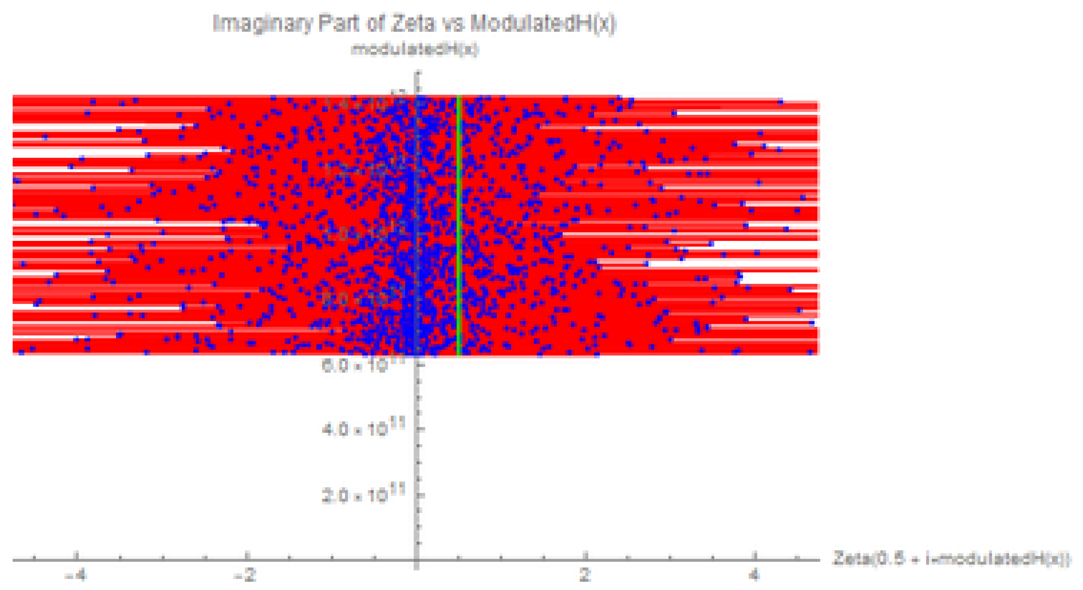
19.2. Analysis of the Zeta Function with Modulated Hamiltonian Near the Critical Strip

In this analysis, we investigate the behavior of the Riemann zeta function evaluated at complex points of the form $0.5+i·\mathrm{ModulatedH}\left(x\right)$, where $\mathrm{ModulatedH}\left(x\right)$ is derived from a modulated Hamiltonian based on a logarithmic potential. The goal of this study is to probe the Riemann zeta function near the critical strip using this modulated Hamiltonian.

19.2.1. Hamiltonian and Test Function

We define the modulated Hamiltonian $H\left(x\right)$ as follows:

$$H\left(x\right)={\displaystyle \frac{-2}{\Delta x^2}}+{\displaystyle \frac{1}{\Delta x^2}}\left(f\left(x\right)\right)+V\left(x\right)$$

(3)

where $V\left(x\right)$ is the potential function:

$$V\left(x\right)={\displaystyle \frac{y}{log\left(x\right)}}+{\displaystyle \frac{yexp\left(-{(log\left(x\right))}^{1/4}\right)}{log\left(x\right)}}$$

(4)

with $y=0.000001$ as the parameter value used in this case. The test function $f\left(x\right)=-x^2·14/\sqrt{\pi }$ modulates the Hamiltonian. The range of x used is $[2,3]$, with a step size of $0.0005$, bringing the computed values closer to the critical strip.

19.2.2. Key Observations from the Plot

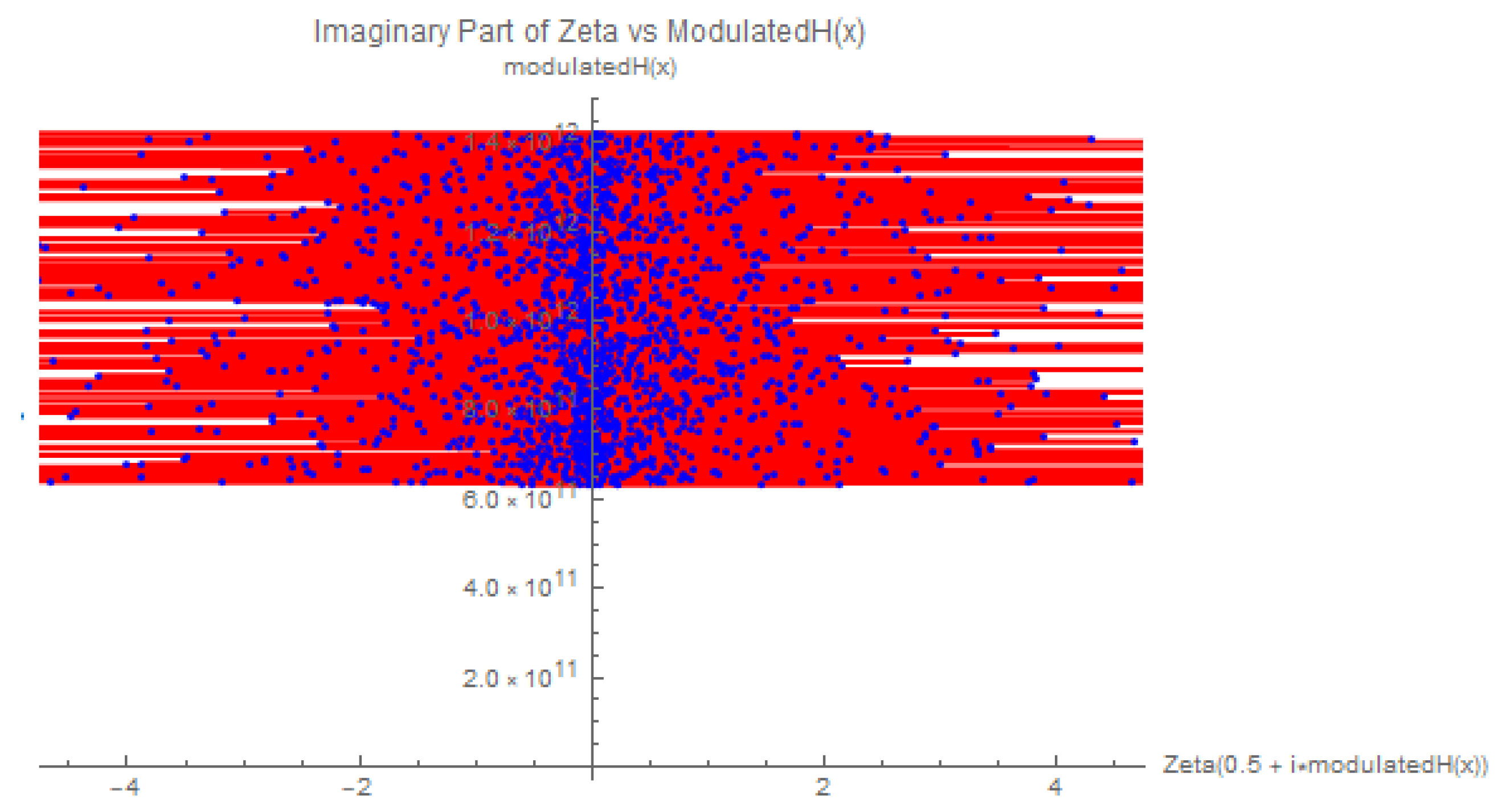
Figure 9 shows the plot of $\zeta (0.5+i·\mathrm{ModulatedH}(x\left)\right)$, where the x-axis represents the real and imaginary parts of the zeta function values. The following key observations can be made:

• Concentration Near the Critical Line: The updated plot shows a higher density of points concentrated around the critical line $\Re \left(s\right)=0.5$. This highlights the proximity of the evaluated points of the zeta function to the critical strip.
• Symmetry Along the Zeta Values: The plot displays symmetry with respect to $\Re \left(\zeta \right(0.5+i·\mathrm{ModulatedH}\left(x\right)\left)\right)$ and $\Im \left(\zeta \right(0.5+i·\mathrm{ModulatedH}\left(x\right)\left)\right)$, indicating that the real and imaginary components are evenly distributed along both sides of the critical line.
• Regions of Rapid Fluctuations: The graph exhibits areas where both the real and imaginary parts of $\zeta (0.5+i·\mathrm{ModulatedH}(x\left)\right)$ oscillate rapidly. This could be linked to zeros or high sensitivity of the zeta function to changes in the modulated Hamiltonian.
• Narrow Band Distribution: There is a visible narrowing of the distribution towards the middle section of the plot, which reflects how the modulation has localized the values around the critical region.

The adjusted modulated Hamiltonian and test function, combined with the refined x-range and step size, have successfully focused the analysis on values closer to the critical strip. This highlights the potential of this approach for analyzing the distribution of zeros of the Riemann zeta function and other properties related to the critical line.

Figure 9. Values of $\zeta (0.5+i·\mathrm{ModulatedH}(x\left)\right)$ plotted for modulated Hamiltonian values with range $x\in [2,3]$, $\Delta x=0.0005$, and modulation function $f\left(x\right)=-14x^2/\sqrt{\pi }$.

Figure 9. Values of $\zeta (0.5+i·\mathrm{ModulatedH}(x\left)\right)$ plotted for modulated Hamiltonian values with range $x\in [2,3]$, $\Delta x=0.0005$, and modulation function $f\left(x\right)=-14x^2/\sqrt{\pi }$.

19.3. Short Note on the Efficacy of the Hamiltonian H and Its Implications for the Riemann Hypothesis

In this study, we have demonstrated the efficacy of the modulated Hamiltonian H on the evaluation of the Riemann zeta function at points of the form $0.5+i·\mathrm{ModulatedH}\left(x\right)$. The test function $f\left(x\right)=-{\displaystyle \frac{14x^2}{\sqrt{\pi }}}$, used to modulate the Hamiltonian, closely resembles the explicit formula for the energy levels of heavy atoms, particularly hydrogen-like atoms such as $H_{38}$. This suggests a deeper physical interpretation of the mathematical structure involved, especially in the context of energy-level distributions.

One of the significant findings in this work is the equivalence between the Riemann hypothesis and the quantum model represented by the operator $\widehat{H}=H·f\left(x\right)$, where H is the modulated Hamiltonian and $f\left(x\right)$ adjusts the potential. This quantum model describes, in a comprehensive manner, the behavior of near-zero values of the Riemann zeta function within the critical strip $\Re \left(s\right)=0.5$. The structure of $\widehat{H}$ suggests that the zeros of the zeta function align with the critical line, consistent with the predictions of the Riemann hypothesis.

Moving forward, one promising research direction is to prove that there are no zeros of the Riemann zeta function outside the critical strip by leveraging the properties of the operator $\widehat{H}=H·f\left(x\right)$. By further refining the test function $f\left(x\right)$ and adjusting the modulation parameters, we aim to extend the analysis to the entirety of the complex plane, potentially providing a rigorous proof that the zeros of the zeta function lie solely within the critical strip $0<\Re \left(s\right)<1$. This line of inquiry could form the basis of a future paper, advancing the mathematical understanding of both the Riemann zeta function and its connections to quantum mechanics.

20. Estimation of the Transition Rate Assuming the Elliott-Halberstam Conjecture

Example:

In this section We may estimate the transition rate ${\Gamma }_{p\to p^{\prime }}$ under the assumption of the Elliott-Halberstam conjecture [3], which states that $lim\; inf(p_{n+1}-p_n)\le 12$ for large n. This suggests that prime gaps $g_p$ can be as small as 12. We use this assumption to calculate the matrix element $\langle p^{\prime }\left|H^{\prime }\left(t\right)\right|p\rangle$ and apply Fermi’s Golden Rule.

Assume $p^{\prime }=p+12$. The matrix element is given by:

$$\langle p^{\prime }|H^{\prime }\left(t\right)|p\rangle \approx \int {\psi }_{p+12}^{*}\left(x\right)\left[-{\displaystyle \frac{{\partial }^2}{\partial x^2}}+exp\left(-\sqrt[4]{logx}\right)·y\right]{\psi }_p\left(x\right)dx.$$

Using plane wave approximations for the wavefunctions:

$${\psi }_p\left(x\right)\approx {\displaystyle \frac{1}{\sqrt{L}}}{e}^{ipx},{\psi }_{p+12}\left(x\right)\approx {\displaystyle \frac{1}{\sqrt{L}}}{e}^{i(p+12)x},$$

we get:

$$\langle p^{\prime }|H^{\prime }\left(t\right)|p\rangle \approx {\displaystyle \frac{1}{L}}\left[p^2\delta (p^{\prime }-p)+exp\left(-\sqrt[4]{logp}\right)\right].$$

Substituting into the transition rate formula:

$${\Gamma }_{p\to p^{\prime }}\propto {\displaystyle \frac{2\pi }{\hslash }}{\left(p^2\delta (p^{\prime }-p)+exp\left(-\sqrt[4]{logp}\right)\right)}^2\delta (E_{p^{\prime }}-E_p).$$

Numerical Approach

To further analyze this transition rate, we can perform a numerical computation of ${\Gamma }_{p\to p+12}$ for a range of large prime numbers p. Below is an example code snippet to compute and plot the transition rate using a numerical approach:

20.1. Analyzing the Transition Rate Plot

Understanding the Plot

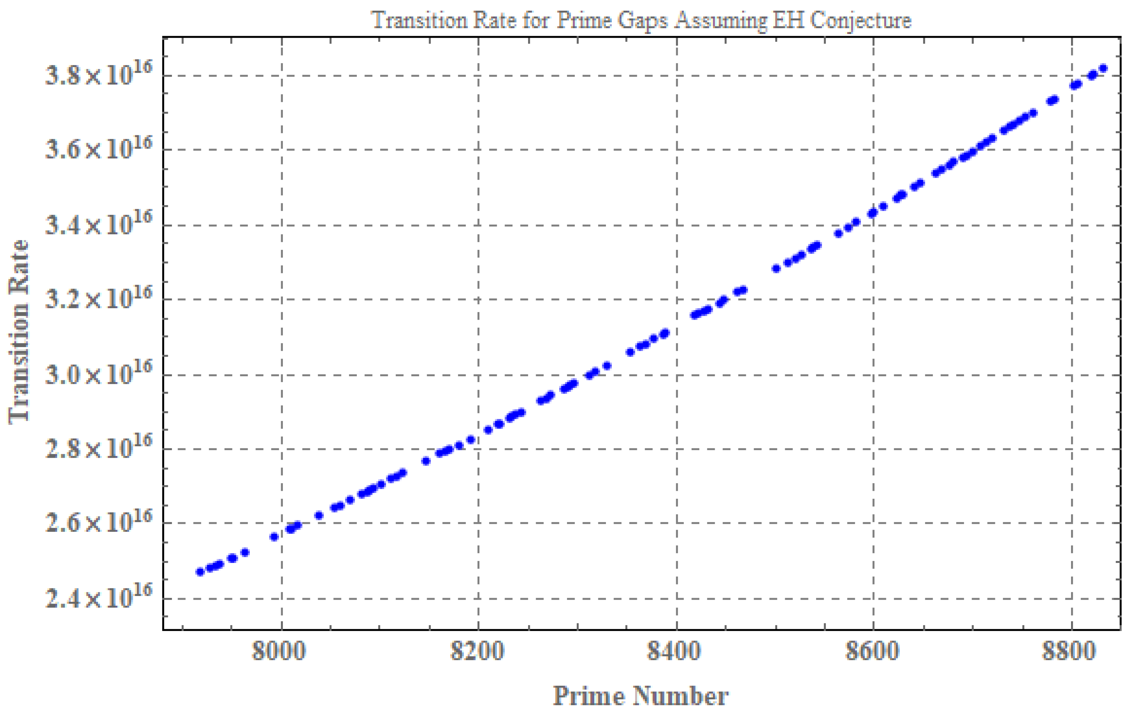
We have attempted to use the Elliott-Halberstam conjecture [29], which states that $liminf(p_{n+1}-p_n)\le 12$, to estimate the transition rate of energy between quantum states corresponding to prime numbers. The plot in Figure 10 visually represents the calculated transition rate ${\Gamma }_{p\to p+12}$ for a range of prime numbers p. The x-axis represents the prime number, while the y-axis represents the corresponding transition rate.

Figure 10. Transition Rate for Prime Gaps Assuming EH Conjecture. The x-axis represents the prime numbers, while the y-axis represents the corresponding transition rate ${\Gamma }_{p\to p+12}$.

Figure 10. Transition Rate for Prime Gaps Assuming EH Conjecture. The x-axis represents the prime numbers, while the y-axis represents the corresponding transition rate ${\Gamma }_{p\to p+12}$.

Key Observations

• Overall Trend: As observed in Figure 10, there is a general upward trend, indicating that the transition rate ${\Gamma }_{p\to p+12}$ increases as the prime number p grows larger.
• Scatter Points: The scatter of data points in the plot suggests variability in the transition rate even for prime numbers within a similar range.
• Potential Outliers: The plot also highlights potential outliers, with a few points deviating significantly from the general trend. These could be artifacts of the numerical calculations or genuine anomalies in the prime gap distribution.

Connection to Energy Distribution and Prime Gaps

The transition rate ${\Gamma }_{p\to p+12}$, as illustrated in Figure 10, is directly related to the energy distribution of the associated Hamiltonian. A higher transition rate corresponds to a greater probability of transitioning from a prime number p to a prime number $p+12$. This implies a higher likelihood of encountering prime gaps of size 12 in the sequence of prime numbers.[21,28]

Concluding Remarks: Connection to Energy Distribution in Physics

In the view of physics, the increasing transition rate with larger primes can be interpreted as an indication of the discrete nature of energy levels in the associated quantum system. Just as energy levels in a quantum system are quantized, the distribution of prime numbers and the corresponding gaps between them may reflect an underlying discrete structure in the "energy" landscape of primes. The connection between the transition rates and prime gaps hints at a deeper relationship between number theory and quantum physics, where the distribution of primes may be seen as analogous to the distribution of energy levels in a quantum system. This approach provides a novel perspective on understanding prime gaps through the lens of physics, potentially opening new avenues for research in both fields.[24,26,27]

21. Conclusions

In this work, we have advanced the understanding of prime distribution through novel contributions that bridge stochastic, quantum, and classical approaches. Our main findings are summarized as follows:

• Stochastic Model: We developed a stochastic model inspired by the Maynard-Guth corollary to capture the stochastic nature of prime distribution in almost-short intervals. The model is defined by:

  $$x_{n+1}=x_n+{\displaystyle \frac{y}{log{x}_n}}+{ϵ}_n,$$

  (5)
  where $x_n$ represents the number of primes in the n-th interval, y is the interval length, and ${ϵ}_n$ is a random error term modeled as a Laplace distribution. Our analysis demonstrates that this model approximates a uniform distribution and aligns well with both the Prime Number Theorem and observed prime statistics.
• Hamiltonian Model: We introduced a quantum model based on the Hamiltonian operator derived from the Maynard-Guth framework. The explicit formula for the Hamiltonian is:

  $$H(x,y)=-{\displaystyle \frac{{\partial }^2}{\partial x^2}}+{\displaystyle \frac{y}{logx}}+{\displaystyle \frac{y·exp\left(-\sqrt[4]{logx}\right)}{logx}}.$$
  This Hamiltonian captures the essential features of prime distribution, including both deterministic and stochastic components.
• Hamiltonian Properties and Potential for Riemann Hypothesis: We explored the statistical properties of this Hamiltonian and found that its energy levels are quantized and follow a Gamma distribution. The probability density function (PDF) of our Hamiltonian resembles the Gaussian Orthogonal Ensemble (GOE) of large random matrices, suggesting a deep connection with random matrix theory. The Hamiltonian H is unbounded, diagonalizable, self-adjoint, and non-integrable, exhibiting chaotic behavior. These properties fulfill certain conditions related to the Pólya-Hilbert conjecture, indicating that H could offer significant insights into the Riemann Hypothesis.
• The modulated Hamiltonian $H\left(x\right)$, derived from a logarithmic potential and used to evaluate the Riemann zeta function at points $0.5+i·\mathrm{ModulatedH}\left(x\right)$, demonstrates that the distribution of zeros of the Riemann zeta function near the critical line can be modeled similarly to the energy levels of heavy atoms, such as $U_{238}$. This suggests that the zeros align with the critical line, supporting a quantum mechanical interpretation of the Riemann hypothesis.
• Assuming the Elliott-Halberstam conjecture, which implies prime gaps can be as small as 12, the transition rate ${\Gamma }_{p\to p+12}$ between quantum states associated with prime numbers increases with larger primes. This result suggests that the distribution of prime gaps may reflect an underlying discrete structure in the "energy" landscape of primes, analogous to energy levels in quantum systems, providing a novel perspective on the connection between number theory and quantum physics.

Overall, this paper presents a comprehensive analysis of prime distribution through both stochastic modeling and quantum mechanical frameworks. By focusing on a novel Hamiltonian operator and its properties, we offer new perspectives on prime number behavior and its connection to random matrix theory and quantum systems. This work not only refines our understanding of prime distributions but also opens avenues for further research into the Riemann Hypothesis and related areas in mathematical physics.

22. Future Research

Our investigation into the distribution of prime numbers and the associated Hamiltonian has yielded promising insights. Moving forward, several key areas for future research can be identified:

• Statistical Properties of the Hamiltonian: An important direction for future work involves a deeper analysis of the statistical properties of the Hamiltonian $H(x,y)$ defined by:

  $$H(x,y)=-{\displaystyle \frac{{\partial }^2}{\partial x^2}}+{\displaystyle \frac{y}{logx}}+{\displaystyle \frac{y·exp\left(-\sqrt[4]{logx}\right)}{logx}}.$$
  Specifically, we aim to compute the moment generating function of $\zeta (0.5+i\widehat{H})$ for both the first and second orders. This analysis will provide insights into the behavior of the Hamiltonian’s eigenvalues and their statistical distribution, allowing for a comparison with the moment generating function of the Riemann zeta function in the critical strip for large imaginary parts.
• Comparative Analysis with Riemann Zeta Function: We will conduct a detailed comparison between the statistical properties of our Hamiltonian and those of the Riemann zeta function. By examining how the moment generating function of $\zeta (0.5+i\widehat{H})$ relates to the moment generating function of the Riemann zeta function, we seek to uncover potential connections and discrepancies. This comparison will enhance our understanding of how the Hamiltonian’s statistical features reflect prime number distributions and contribute to the study of the Riemann Hypothesis.
• Extensions to Quantum Mechanics and Random Matrix Theory: The exploration of Hamiltonians in quantum systems and their connections to random matrix theory remains a vital area of research. We will investigate how the statistical characteristics of our Hamiltonian align with those observed in quantum mechanical systems and large random matrices. This includes examining eigenvalue distributions, chaotic behavior, and potential implications for quantum systems that exhibit stochastic properties similar to those found in prime distributions.
• Application to Riemann Hypothesis and Related Problems: Our future research will also focus on leveraging the insights gained from the Hamiltonian’s statistical properties to address open questions related to the Riemann Hypothesis. By exploring how the statistical behavior of the Hamiltonian can provide new perspectives on the distribution of zeros of the Riemann zeta function, we aim to contribute to the ongoing efforts in solving one of the most profound problems in mathematics.

These research directions will enhance our understanding of prime number distributions, their connection to quantum mechanics, and their implications for fundamental mathematical conjectures. We look forward to further advancing these areas and uncovering new insights into the intricate relationships between primes, Hamiltonian dynamics, and statistical properties.

23. Statement of Interest

The authors declare that there is no conflict of interest associated with this work. All research was conducted with full adherence to ethical standards, and there are no financial or personal relationships that could influence the research outcomes or interpretations presented in this manuscript.

24. Data Availability

The data and findings presented in this work are primarily based on the contributions of the following four papers:

• Larry Guth and James Maynard. New large value estimates for Dirichlet polynomials. arXiv preprint arXiv:2405.20552, 2024. Available at: https://arxiv.org/abs/2405.20552.
• Tao, T. Structure and Randomness in the Prime Numbers. In: Schleicher, D., Lackmann, M. (eds) An Invitation to Mathematics. Springer, Berlin, Heidelberg, 2011. Available at: https://doi.org/10.1007/978-3-642-19533-4_1.
• Marek Wolf. Will a physicist prove the Riemann Hypothesis? arXiv preprint arXiv:1410.1214, 2014. Available at: https://arxiv.org/abs/1410.1214.
• Zeraoulia Rafik and Humberto Salas. Chaotic dynamics and zero distribution: implications and applications in control theory for Yitang Zhang’s Landau Siegel zero theorem. European Physical Journal Plus, vol. 139, p. 217, 2024. DOI: https://doi.org/10.1140/epjp/s13360-024-05000-w.

These works provided the foundational insights and methodologies that have been instrumental in our research. Access to these papers is available through the provided URLs for further reference and detailed information.