
Submitted:
13 September 2024
Posted:
16 September 2024
You are already at the latest version
Abstract
The paper addresses the challenging issue of trajectory tracking for uncertain quadrotor UAVs, particularly under the constraints of input saturation and external disturbances. It introduces adaptive laws for managing uncertainties in mass and inertia moments without requiring prior knowledge, ensuring effective control even with varying system parameters. To counteract the effects of input saturation, the study incorporates an auxiliary system designed to compensate for these limitations. Additionally, a disturbance observer(DO) is utilized to manage and mitigate the impact of time-varying external disturbances. The proposed control strategy integrates a sliding mode adaptive control approach with an inner-outer loop structure, enhancing robustness and adaptability. Numerical simulations demonstrate the effectiveness of the designed control strategy.
Keywords:
trajectory tracking control
; sliding mode control
; disturbance observer
; input saturation
; parametric uncertainties
1. Introduction
In recent years, the UAVs has gained widespread applications in areas such as aerial photography [1], emergency communication [2], and agricultural irrigation [3]. Its popularity arises from its small size, affordability, and simple structure. Nevertheless, the demanding task scenarios faced by these quadrotor UAVs improved performance against internal and external disturbances. Moreover, as an underactuated and nonlinear coupled system, traditional control methods face challenges in achieving high-precision control amidst disturbances. Consequently, there is a critical emphasis on developing anti-disturbance methods in control theory and application.
In parallel, the sliding mode control method, known for its robust characteristics, insensitivity to disturbances, and rapid response, offers another avenue for achieving precise control in UAVs [4]. Recent studies, such as [5,6,7,8,9], have explored and demonstrated the effectiveness of sliding mode control algorithms in addressing trajectory tracking challenges and improving the overall robustness of quadrotor UAVs. This control method facilitates system movement along the designated sliding mode surface, with an adjustable convergence rate by selecting the sliding mode surface parameter matrix. Owing to the model’s lower precision, this control method has been user-friendly and widely applied in UAV control [10]. A novel fractional-order non-singular fast terminal sliding mode surface is proposed In [11], specifically designed for precise quadrotor trajectory tracking. Through simulations, the approach demonstrates its enhanced performance in suppressing external disturbances, significantly improving the quadrotor’s stability during flight. Additionally, the method ensures accurate trajectory following, even in the presence of uncertainties, making it an effective solution for high-precision applications. In [12], an iterative learning sliding mode control algorithm was developed, with experimental results confirming its effectiveness in achieving precise trajectory tracking while maintaining robustness against disturbances.
The disturbance observer technique, first introduced in 1987 [13], has proven to be an effective method for suppressing external disturbances in various control systems. Its design involves constructing a dynamic system that estimates unknown disturbances based on known system parameters and behavior. By accurately estimating these disturbances in real-time, the observer allows for the design of a robust compensation term that actively counteracts their effects. This proactive disturbance rejection mechanism greatly enhances the overall performance and stability of control systems, making the technique particularly valuable in environments with significant external disruptions. Due to its clear physical significance and simple design structure, combining disturbance observers with other control methods has become a crucial approach for addressing system uncertainty issues. A comprehensive method and fundamental framework for handling disturbance in nonlinear systems using a disturbance observer were introduced in [14], and the approach extends the traditional disturbance observer-based control strategy, which is typically applied to linear systems, to more complex nonlinear systems. In [15], a composite controller that integrates a disturbance observer with the backstepping method, specifically designed for nonlinear systems subjected to bounded disturbances was developed, enhancing overall system performance and disturbance rejection. An anti-disturbance control strategy was implemented in [16] for an indoor quadrotor UAV system, incorporating a disturbance observer to manage and counteract external disturbances, effectively mitigating the effects of modeling errors and external disturbances to improve system stability and accuracy.
In many cases, the output of an actuator cannot consistently increase due to its physical constraints, resulting in an input saturation problem. Prolonged influence of input saturation accelerates the damage to the actuator, necessitating consideration of this factor in controller design. Currently, there are three primary approaches to address the input saturation problem: The first approach involves using a small gain controller to reduce the amplitude of control inputs, effectively preventing the system from reaching saturation limits [17]. The second approach approximates the nonlinear behavior of input saturation with a smooth function, allowing for a more continuous and manageable control response [18]. Finally, a dynamic auxiliary system can be designed to compensate for saturation effects, actively adjusting the control signals to maintain performance even when inputs are constrained [19]. Based on the boundedness of the hyperbolic tangent function, a quasi-proportion-integral-derivative (PID) control strategy was proposed in [17], ensuring that the sum of the control gains is kept below the saturation upper limit to avoid input saturation. However, determining appropriate control gains remains a highly challenging task. An Nussbaum function was incorporated into the design process of the backstepping method [18], addressing input saturation and avoiding potential singularities during attitude stabilization. Nonetheless, the physical structure and design process of this controller are exceedingly complex. An anti-saturation scheme employing a dynamic auxiliary system that effectively mitigates the impact of input saturation within finite time, ensuring system convergence and stability, was designed in [19]. Moreover, the dynamic auxiliary system does not compromise controller performance when input saturation is absent.
During the flight of quadrotor UAVs, challenges arise not only from wind disturbances and mismatched disturbances but also from model uncertainties, posing a potential threat to overall system stability. Utilizing adaptive control laws offers a solution by approximating unknown upper bounds, enabling compensation for model parameter uncertainties within the controlled system. In [20], an adaptive sliding mode control method that integrated smooth and continuous integrators was explored. This method was specifically crafted for tracking control amid uncertainties and disturbances in aircraft. In [21], a control approach was implemented to enhance the resistance of quadrotor UAVs to wind disturbances. This study implements an adaptive fuzzy PID control system aimed at improving both the stability and tracking performance of the quadrotor UAV. In summary, the adaptive rate provides a promising avenue for UAVs to address model uncertainties.
Building upon the preceding discussions on control methodologies, the present study investigates the trajectory tracking challenges faced by a quadrotor UAV amid input saturation, external disturbances and parametric uncertainty. The key contributions of this article are as follows.
- An adaptive sliding mode trajectory tracking controller is proposed for the uncertain QUAV, ensuring globally uniformly ultimate boundedness(UUB) despite disturbances, input saturation, and parameter uncertainties.
- To address parameter uncertainties, adaptive laws are developed to estimate the quadrotor’s mass and unknown constants related to the moment of inertia. These adaptive laws are integrated into the control scheme, allowing the controller to compensate for external disturbances and input saturation without requiring prior knowledge of the quadrotor’s physical properties.
- The method also incorporates disturbance observers and auxiliary systems, designed to function without prior knowledge of the quadrotor’s mass and moments of inertia. This enables the system to effectively handle unknown disturbances and input saturation, ensuring robust adaptive path tracking performance under uncertain conditions.
The paper is structured as follows: Section 2 lays the foundation by establishing the mathematical model for the quadrotor UAV, providing the necessary framework for control system design. Section 3 develops sliding mode control laws for both position and attitude loops, addressing key challenges such as input saturation, external disturbances, and parametric uncertainties, followed by a subsequent stability analysis. Section 4 presents the simulation results, demonstrating the practical performance of the proposed control strategies in overcoming these challenges, with conclusions drawn in the dedicated section 5.
2. Mathematical Model of Quadrotor
The position of the UAV is represented by the vector , while the attitude angles are expressed by the vector , where P denotes the spatial coordinates, and represents the pitch, roll, and yaw angles, respectively. Considering the external disturbance, the nonlinear dynamic system of quadrotor can be expressed as follows [22]
where m is the mass of the UAV, g is the gravitational acceleration, l is the distance of the quadrotor’s center of mass to any of the rotor’s rotation axis, , , and are airframe inertia of roll, pitch and yaw, respectively, represents the external disturbances of each channel.
The definition of the virtual control input is provided herewith for the purpose of facilitating the design of control rates. In practical scenarios, the rotor moment of a quadrotor UAV is subject to physical constraints during flight, limiting the extent to which control inputs can be applied. To accurately reflect these limitations, the following saturation function is used in the control strategy to ensure that the control inputs remain within the feasible range [23]
where is the ith control input of the system, is the upper bound of the ith control input and .
Define . Then, the position subsystem of the quadrotor is written as the following affine nonlinear form
where represent the saturation input to the position subsystem, represent the unknown external disturbances in position subsystem, and is the system state vector and the control gain, respectively.
Similarly, define , the attitude subsystem of the quadrotor is written as
where represent the saturation input to the attitude subsystem, represent the unknown external disturbances in attitude subsystem. The system state vector is
Control gain matrix is
And and are constants in (5) and (6), which are written as follows
Due to the difficulty in accurately measuring the mass and inertia moments of a quadrotor UAV, is used in place of and is used in place of in the subsequent controller design stages. Meanwhile, the development of adaptive sliding mode tracking controllers for QUAV relies on the following specific lemmas and assumptions.
Lemma 1.
[24] Consider the following equation which describes an affine nonlinear system
where is the vector of state, is the vector of disturbance, and are the system input and output, respectively. Disturbance observer is designed as
where z, u, and are auxiliary variable, control input, disturbance estimation, and nonlinear function, respectively. The gain are calculated as
choosing to make it satisfied , then the disturbance estimation error , as defined below
is guaranteed to converge globally exponentially.
Lemma 2.
The command filter is [25]
The signal satisfies and , where , are positive constants and the initial conditions are set as . Under these conditions, for any , there exist , such that , along with the first and second derivatives are bounded.
Assumption 1.
[26] Assuming that the external disturbance and are slow time-varying signals. They are bounded by positive constant and , respectively, that is for , and .
Assumption 2.
[27] The reference signals , , and , along with their derivatives, are continuous and bounded.
3. Control Design
The quadrotor UAVs are inherently characterized by their high nonlinearity and underactuation. Therefore, it is impossible for quadrotor UAVs to simultaneously track all six degrees of freedom. Accordingly, the primary control objective for the UAV is to accurately track a specified trajectory and yaw angle , while ensuring the stability of the other two angles.
3.1. Position Subsystem Adaptive Control
For position subsystem described by (4), Its tracking target is designed as . Assuming that the desired signal are . To overcome the adverse effects of external disturbance, it is first necessary to design a DO to compensate for it. A generalized form of DO is designed according to Lemma 1, which requires the calculations for . Choose
where
is the designed parameter and satisfies . Then, invoking (4) and (13) in Equation (9), the DO is written as
Combining Assumption 1 with Equation (11), the derivative of the disturbance estimation error is derived as
To address the issue of input saturation in the uncertain UAV position subsystem (3), the detrimental effects of input saturation are tackled by constructing the following auxiliary systems [28]
where is the state, is the designed positive definite matrix and . In the real world, actuators have finite energy, making it necessary to ensure that is constrained by , where is a positive parameter. This finite energy constraint ensures that the control inputs remain within feasible limits, allowing the system to remain controllable while protecting the actuators from excessive load.
A sliding mode surface is proposed as
where and
The designed parameter matrix satisfies condition . The aim is to get the error as close to zero as possible. Taking the derivative of Equation (19)
According to (20), the virtual controller is designed as
where is the parameter matrix to be designed, and represents the estimate of the inverse of the mass and the output of the DO, respectively. The estimation error of the mass inverse is
The adaptive law is designed as [29]
where and are the constant to be designed. The estimate is projected to the interval using the projection operator, which is expressed as
Redefine a variable that includes the estimation error and as follows
And the derivative of (25) can be obtained from (11) and (22) as
Consider the Lyapunov function candidate
Invoking (4), (17), (18), (21), (22) and (24), the time derivative of is
where
To ensure system stability, it is essential to ensure that the appropriate design matrices and parameters .
In conclusion, the signals , the estimate errors , , the variables of the auxiliary system states , are all bounded, the drone’s position is able to keep up with the desired signals.
3.2. Attitude Subsystem Adaptive Control
To achieve the desired tracking targets, namely , the actual lift and attitude subsystem intermediate command signals and must first be calculated. The inverse solution according to (2) yields written as follows [27]
Defining that the desired signal are , . where the derivative of can be obtain from Lemma 2. According to Lemma 1, we have
where
is the designed parameter matrix and satisfies . Invoking (5) and (30) in (10), the DO is written as
where
Similarly, the attitude subsystem is susceptible to input saturation, which can be addressed by constructing a system in the same form as the auxiliary system described above. This approach can effectively compensate for the effects of input saturation.[28]
where is the state, is the designed positive definite matrix and . The sliding mode surface is also defined in the form of (19)
where and
The designed parameter matrix satisfies condition . The controller of the attitude subsystem is proposed as
where is the parameter matrix to be designed, and represents the estimate of the inverse of the inertia matrix and the output of the DO, respectively. In this control rate, the derivatives of the two intermediate control signals and generated by the outer loop can be derived from Lemma 2. The estimation error of the inverse of the inertia are defined as follows
The adaptive law is designed as [29]
where and are designed positive constants. The estimate is projected to the interval using the projection operator, which is expressed as
Redefine that includes the estimation error and as follows
For the whole attitude subsystem, taking the following Lyapunov function
Then
where
Thus, the signal , and are all bounded. To conduct comprehensive stability analysis of the quadrotor, a stability function is defined as
Taking derivative of (46), we can obtain
where
Accordingly, the UAV is able to perform trajectory tracking tasks and achieve control objectives.
4. Simulation Study
Numerical simulations were performed to validate the proposed control strategy, employing a quadrotor UAV model that was subjected to both input saturation and two distinct types of external disturbances. These simulations provided a rigorous test of the control strategy’s performance under challenging conditions. The UAV and controller parameters used in the simulations are comprehensively detailed in Table 1 and Table 2, respectively. The parameters presented in the table are all expressed in International System of Units.
A. Robustness to Constant Disturbances
The reference trajectory signals are expected trajectory and expected yaw Angle are
The initial position and attitude states of the quadrotor are assumed to be . The external disturbances conforming to the hypothesis are: at ; at ; at ; at ; at ;, at . The thrust and the torque of the UAV are limited in and , respectively.
Figure 1 presents a three-dimensional plot showing the expected trajectory tracking of the quadrotor UAV in accordance with the methodology proposed in this paper. Figure 2 and Figure 3 depict the position and attitude tracking processes of the UAV, highlighting the controller’s ability to maintain performance even in the presence of disturbances. It can be observed that when the disturbances are small, the tracking performance is not significantly affected. However, under larger disturbances, the UAV’s z and channels deviate noticeably from the desired trajectory but quickly realign. Overall, the designed controller effectively counters external disturbances and achieves the intended tracking objectives, ensuring stable and accurate performance under varying conditions.
Figure 4 presents the input torques of the UAV, while Figure 5 illustrates the outputs of the disturbance observers across the six channels. The disturbance observer is shown to accurately capture the magnitude of the disturbances affecting the system. These observations confirm the effectiveness of the disturbance observer in mitigating the adverse impacts of external disturbances on the quadrotor UAV. As a result, the disturbance observer enhances the UAV’s overall performance and stability, ensuring more reliable and robust operation under challenging conditions. All the results show that the UAV is able to overcome the effects of constant value disturbances and perform the trajectory tracking task with limited inputs.
B. Robustness to Time-Varying Disturbances
In most cases, the external disturbances are variable. Therefore, a second experimental test with the following objectives is designed
where
And
The initial position and input limits of the UAV in this experiment are consistent with those used in previous tests. The experimental outcomes, illustrated in Figure 6, Figure 7 and Figure 8, highlight the UAV’s ability to maintain accurate trajectory tracking even in the presence of time-varying disturbances. Despite these dynamic disturbances, the UAV successfully maintains accurate tracking of the target path. The conclusions drawn from this experiment confirm the robustness and stability of the UAV’s control strategy, demonstrating its effectiveness in managing external disturbances while ensuring precise and reliable trajectory tracking.
The output of the drone torque is also well limited to the preset range as seen in Figure 9. Additionally, Figure 10 highlights the capability of the disturbance observer to accurately estimate both the amplitude and frequency of time-varying disturbances, despite their dynamic nature. These findings confirm that the control system successfully maintains the drone’s torque within specified limits and that the disturbance observer provides precise estimations of dynamic disturbances. As a result, the overall robustness and performance of the UAV are significantly enhanced, demonstrating the effectiveness ofthe integrated control and estimation strategies.
The combination of the two aforementioned cases leads to the conclusion that, in the absence of knowledge regarding the mass and moment of inertia of the UAV, and in the presence of input saturation, the force and torque required by the UAV remain within a reasonable range, irrespective of whether the disturbance in question is constant or time-varying. Furthermore, the DO is capable of accurately estimating the magnitude of external disturbances and compensating for them in a manner that is relayed to the controller. This ultimately renders the UAV both robust and capable of excelling in the completion of trajectory tracking tasks.
5. Conclusions
The paper presents a tracking control method for quadrotor UAVs that effectively handles parametric uncertainties, external disturbances, and input saturation, without requiring prior knowledge of the UAV’s mass or moments of inertia. This adaptability allows the control system to perform well under various conditions. Simulations validate the effectiveness of the proposed approach and demonstrate its robustness to various disturbances and uncertainties. Furthermore, the method offers significant advantages over existing control techniques by addressing multiple factors simultaneously, providing a more comprehensive solution for ensuring reliable and accurate trajectory tracking in real-world applications.
Author Contributions
Conceptualization, J.K. and M.C.; methodology, J.K.; software, J.K.; validation, J.K. and M.C.; writing—original draft preparation, J.K.; writing—review and editing, M.C.; supervision, M.C. All authors have read and agreed to the published version of the manuscript.
Funding
This research received no external funding.
Data Availability Statement
The data are contained within the article.
Conflicts of Interest
The authors declare no conflicts of interest.
References
- Kendoul, F.; Yu, Z.; Nonami, K. "Guidance and nonlinear control system for autonomous flight of minirotorcraft unmanned aerial vehicles". Journal of Field Robotics 2010, 27, 311–334. [CrossRef]
- Nagaty, A.; Saeedi, S.; Thibault, C.; Seto, M.; Li, H. "Control and navigation framework for quadrotor helicopters". Journal of intelligent & robotic systems 2013, 70, 1–12. [CrossRef]
- Gupte, S.; Mohandas, P.I.T.; Conrad, J.M. "A survey of quadrotor unmanned aerial vehicles". 2012 Proceedings of IEEE Southeastcon 2012, pp. 1–6. [CrossRef]
- Antonio-Toledo, M.E.; Sanchez, E.N.; Alanis, A.Y.; Flórez, J.; Perez-Cisneros, M.A. "Real-time integral backstepping with sliding mode control for a quadrotor UAV". IFAC-PapersOnLine 2018, 51, 549–554. [CrossRef]
- Jia, Z.; Yu, J.; Mei, Y.; Chen, Y.; Shen, Y.; Ai, X. "Integral backstepping sliding mode control for quadrotor helicopter under external uncertain disturbances". Aerospace Science and Technology 2017, 68, 299–307. [CrossRef]
- Zhou, L.; Zhang, J.; Dou, J.; Wen, B. "A fuzzy adaptive backstepping control based on mass observer for trajectory tracking of a quadrotor UAV". International journal of adaptive control and signal processing 2018, 32, 1675–1693. [CrossRef]
- Labbadi, M.; Cherkaoui, M. "Robust adaptive backstepping fast terminal sliding mode controller for uncertain quadrotor UAV". Aerospace Science and Technology 2019, 93, 105306. [CrossRef]
- Zhang, J.; Ren, Z.; Deng, C.; Wen, B. "Adaptive fuzzy global sliding mode control for trajectory tracking of quadrotor UAVs". Nonlinear Dynamics 2019, 97, 609–627. [CrossRef]
- Razmi, H.; Afshinfar, S. "Neural network-based adaptive sliding mode control design for position and attitude control of a quadrotor UAV". Aerospace Science and technology 2019, 91, 12–27. [CrossRef]
- Xiong, J.J.; Zheng, E.H. "Position and attitude tracking control for a quadrotor UAV". ISA transactions 2014, 53, 725–731. [CrossRef]
- Labbadi, M.; Cherkaoui, M. "Adaptive fractional-order nonsingular fast terminal sliding mode based robust tracking control of quadrotor UAV with Gaussian random disturbances and uncertainties". IEEE Transactions on Aerospace and Electronic Systems 2021, 57, 2265–2277. [CrossRef]
- Nguyen, L.V.; Phung, M.D.; Ha, Q.P. "Iterative learning sliding mode control for UAV trajectory tracking. Electronics 2021, 10, 2474. [CrossRef]
- Ohnishi, K. "A new servo method in mechatronics". Trans. of Japanese Society of Electrical Engineering, D 1987, 177, 83–86.
- Chen, W.H. "Disturbance observer based control for nonlinear systems". IEEE/ASME transactions on mechatronics 2004, 9, 706–710. [CrossRef]
- Zhang, H.; Wei, X.; Karimi, H.R.; Han, J. "Anti-disturbance control based on disturbance observer for nonlinear systems with bounded disturbances". Journal of the Franklin Institute 2018, 355, 4916–4930. [CrossRef]
- Wang, H.; Chen, M. "Trajectory tracking control for an indoor quadrotor UAV based on the disturbance observer". Transactions of the Institute of Measurement and Control 2016, 38, 675–692. [CrossRef]
- Sun, N.; Yang, T.; Fang, Y.; Wu, Y.; Chen, H. "Transportation control of double-pendulum cranes with a nonlinear quasi-PID scheme: Design and experiments". IEEE Transactions on Systems, Man, and Cybernetics: Systems 2018, 49, 1408–1418. [CrossRef]
- Wang, R.; Liu, J. "Trajectory tracking control of a 6-DOF quadrotor UAV with input saturation via backstepping". Journal of the Franklin Institute 2018, 355, 3288–3309. [CrossRef]
- Liu, K.; Wang, X.; Wang, R.; Sun, G.; Wang, X. "Antisaturation finite-time attitude tracking control based observer for a quadrotor". IEEE Transactions on Circuits and Systems II: Express Briefs 2020, 68, 2047–2051. [CrossRef]
- Castañeda, H.; Rodriguez, J.; Gordillo, J.L. "Continuous and smooth differentiator based on adaptive sliding mode control for a quad-rotor MAV". Asian Journal of Control 2021, 23, 661–672. [CrossRef]
- Simoud, L.; Kadri, B.; Bousserhane, I.K. "Adaptive fuzzy-sliding mode controller for trajectory tracking control of quad-rotor". Journal of Automation Mobile Robotics and Intelligent Systems 2020, 14, 15–24. [CrossRef]
- Guo, Y.; Wu, M.; Tang, K.; Wang, X. "Integral back-stepping algorithm for designing the quadrotor aircraft controller". Chin. J. Intell. Sci. Technol 2019, 1, 133–139.
- Li, Y.; Tong, S.; Li, T. "Adaptive fuzzy output-feedback control for output constrained nonlinear systems in the presence of input saturation". Fuzzy Sets and Systems 2014, 248, 138–155. [CrossRef]
- Li, S.; Yang, J.; Chen, W.H.; Chen, X. "Disturbance observer-based control: methods and applications"; CRC press, 2014.
- Yu, J.; Shi, P.; Dong, W.; Yu, H. "Observer and command-filter-based adaptive fuzzy output feedback control of uncertain nonlinear systems". IEEE Transactions on Industrial Electronics 2015, 62, 5962–5970. [CrossRef]
- Pu, M.; Wu, Q.; Jiang, C.; Cheng, L. Application of adaptive second-order dynamic terminal sliding mode control to near space vehicle. Journal of Aerospace Power 2010, 25, 1169–1176.
- Zhang, R.; Ji, H. Robust Adaptive Trajectory Tracking Control for Uncertain Quadrotor Unmanned Aerial Vechicles in the Presence of Actuator Saturation. In Proceedings of the 2020 5th International Conference on Control and Robotics Engineering (ICCRE). IEEE, 2020, pp. 104–108. [CrossRef]
- Yang, Q.; Chen, M. "Adaptive neural prescribed performance tracking control for near space vehicles with input nonlinearity". Neurocomputing 2016, 174, 780–789. [CrossRef]
- Boskovic, J.D.; Chen, L.; Mehra, R.K. "Adaptive control design for nonaffine models arising in flight control". Journal of guidance, control, and dynamics 2004, 27, 209–217. [CrossRef]
Figure 1.
3D trajectory tracking effect
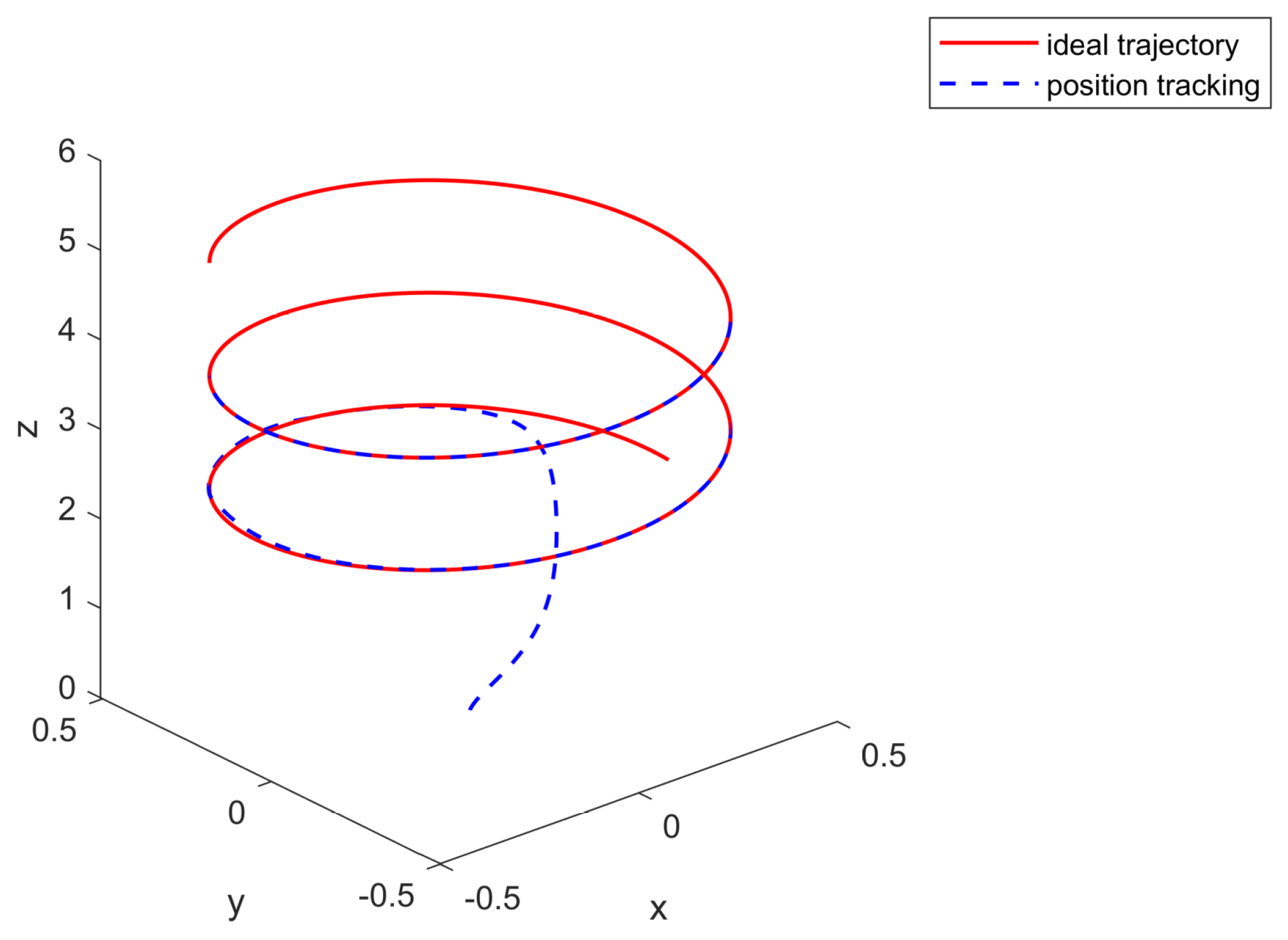
Figure 2.
position tracking
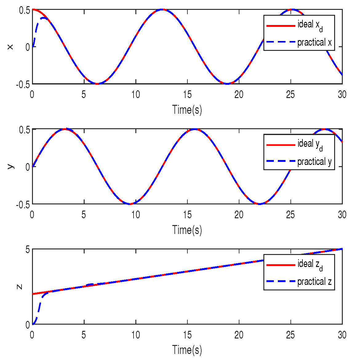
Figure 3.
attitude angle tracking
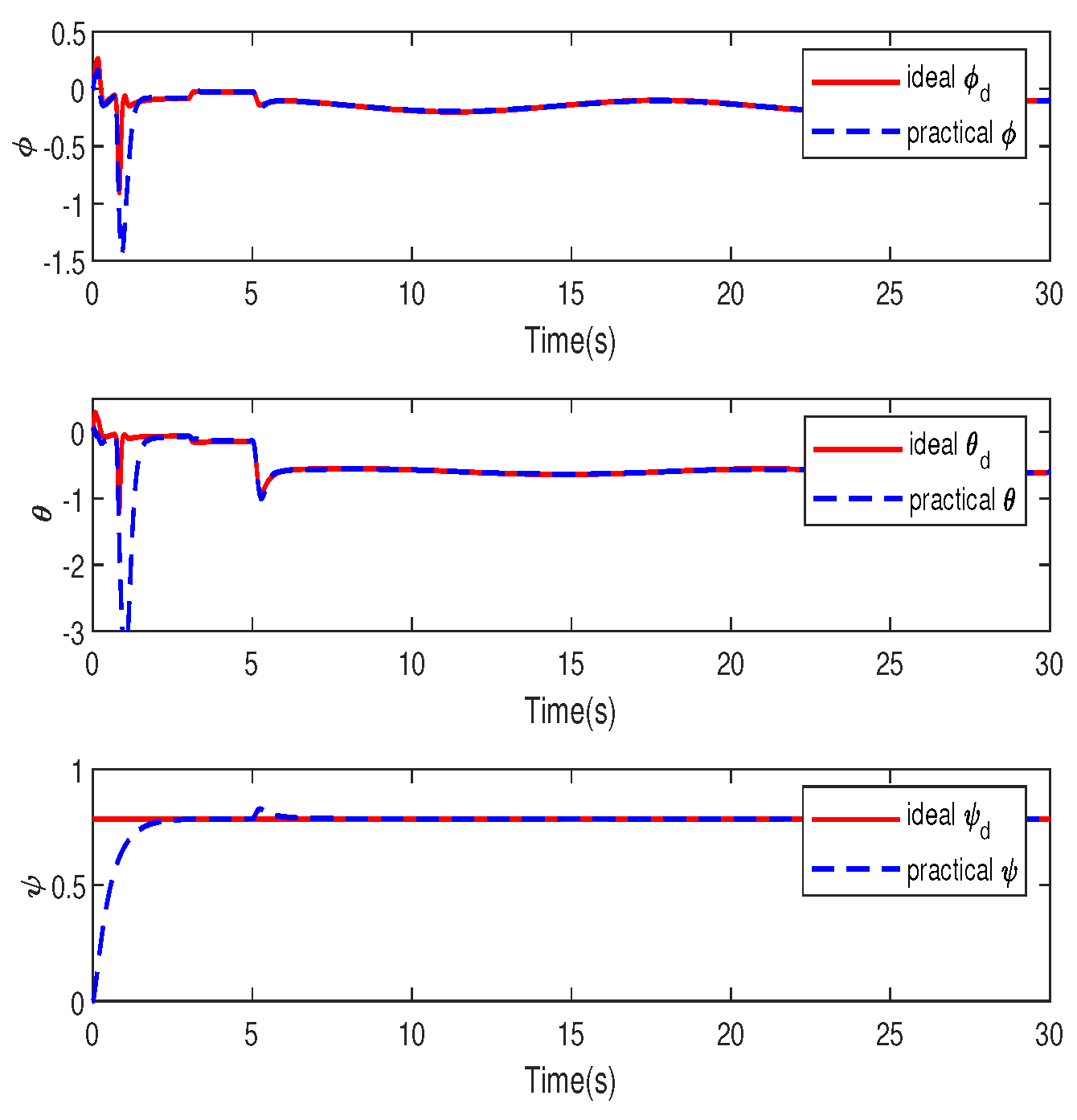
Figure 4.
control input
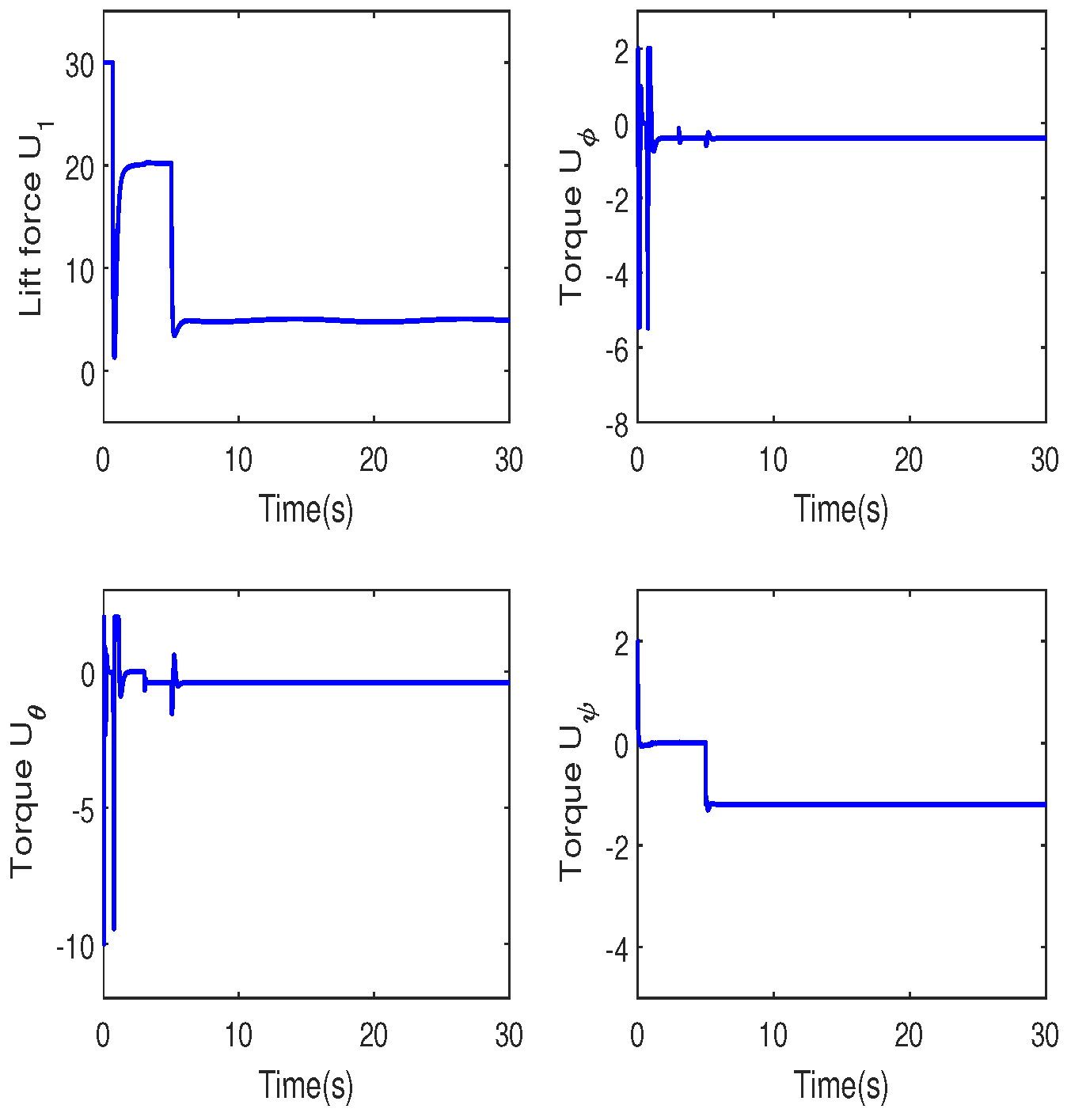
Figure 5.
output of disturbance observer
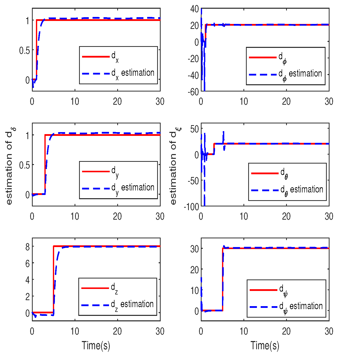
Figure 6.
3D trajectory tracking effect
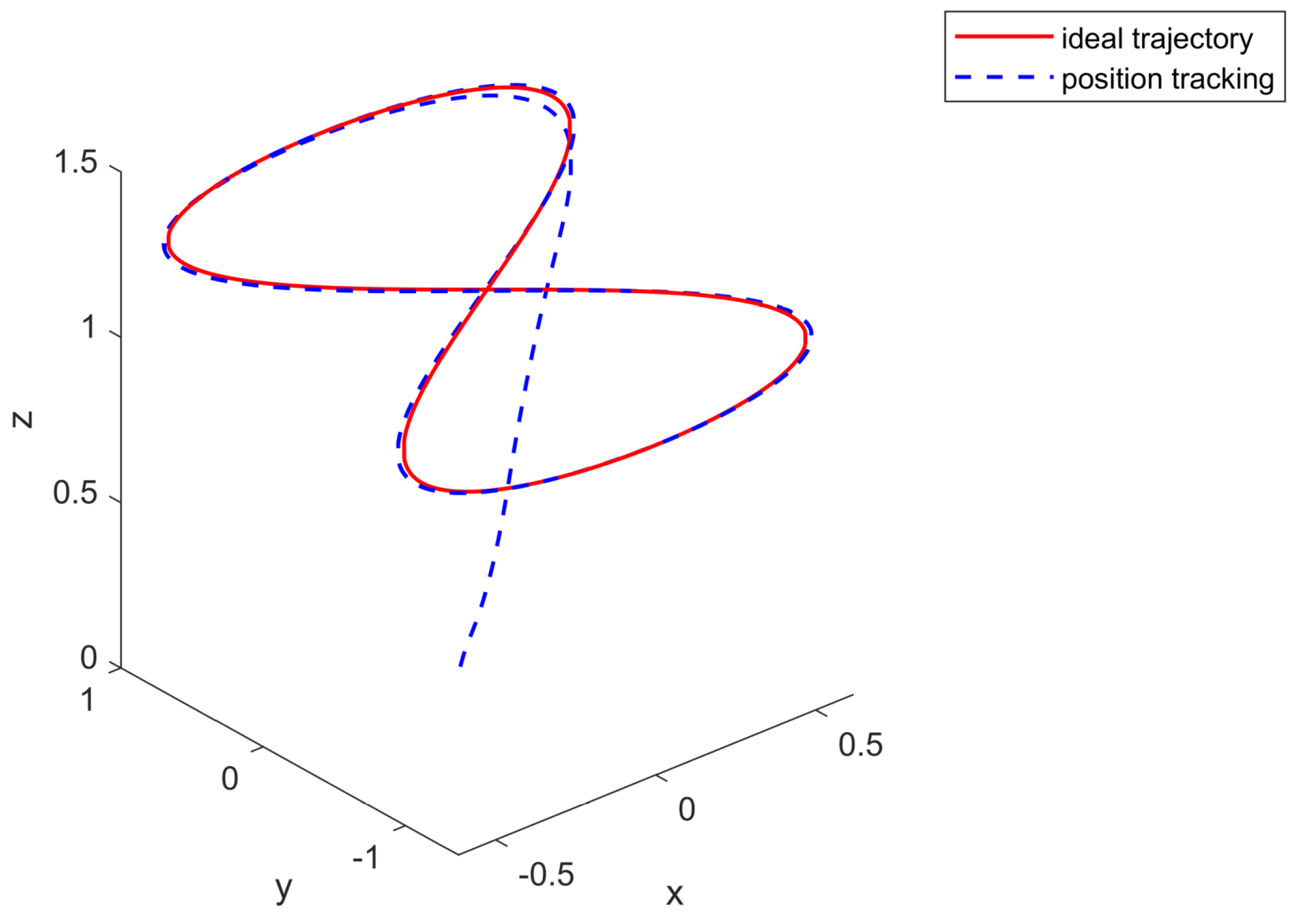
Figure 7.
position tracking
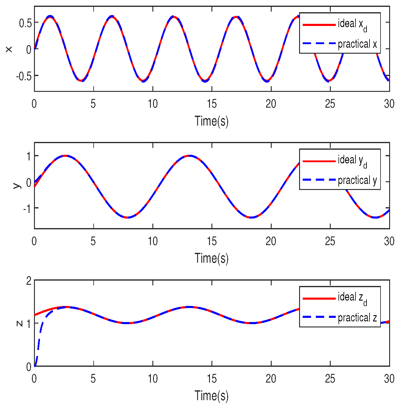
Figure 8.
attitude angle tracking
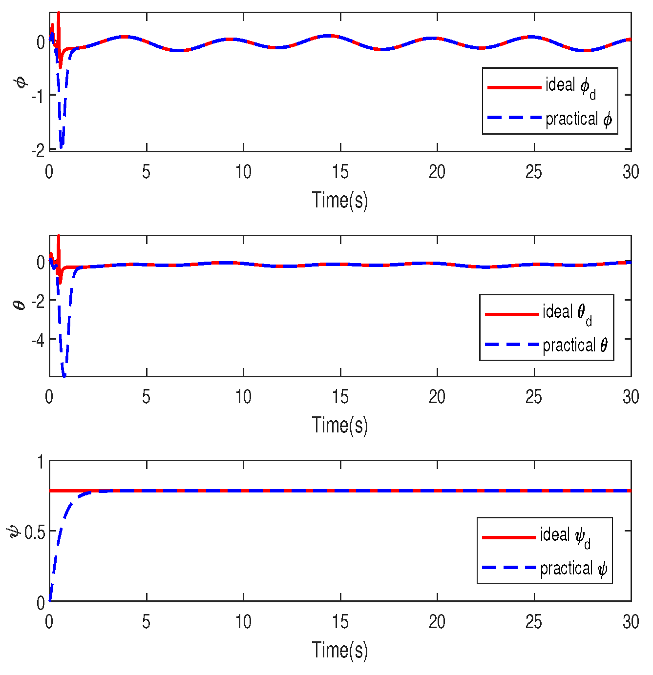
Figure 9.
control input
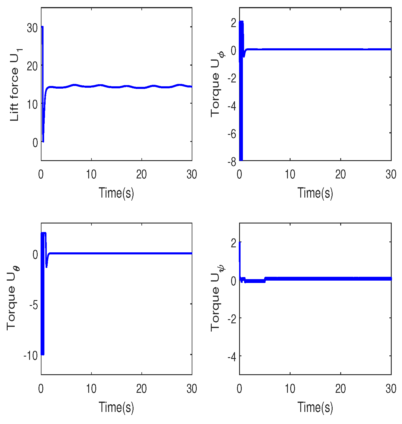
Figure 10.
output of disturbance observer
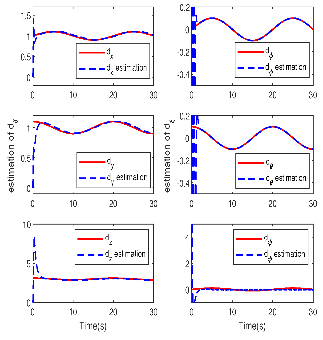

Table 1.
UAV parameters.
| parameter | Symbol | Magnitude |
|---|---|---|
| Mass | m | 2 |
| Airframe inertia of roll | Jx | 0.02 |
| Airframe inertia of pitch | Jy | 0.02 |
| Airframe inertia of yaw | Jz | 0.04 |
| Distance | l | 0.2 |
| Gravity | g | 9.8 |
Table 2.
SMC and DO parameters.
| parameter | Magnitude |
|---|---|
| diag([2 2 2]) | |
| diag([20 20 20]) | |
| diag([2 2 2]) | |
| diag([10 10 10]) | |
| diag([15 15 15]) | |
| [0.2 0.2 0.2 0.2] | |
| [0.5 0.5 0.5 0.5] | |
| diag([18 18 18]) | |
| diag([30 30 30]) | |
| diag([5 5 5]) | |
| diag([10 10 10]) | |
| diag([15 15 15]) |
Disclaimer/Publisher’s Note: The statements, opinions and data contained in all publications are solely those of the individual author(s) and contributor(s) and not of MDPI and/or the editor(s). MDPI and/or the editor(s) disclaim responsibility for any injury to people or property resulting from any ideas, methods, instructions or products referred to in the content. |
© 2024 by the authors. Licensee MDPI, Basel, Switzerland. This article is an open access article distributed under the terms and conditions of the Creative Commons Attribution (CC BY) license (http://creativecommons.org/licenses/by/4.0/).
Copyright: This open access article is published under a Creative Commons CC BY 4.0 license, which permit the free download, distribution, and reuse, provided that the author and preprint are cited in any reuse.


