
Submitted:
11 September 2024
Posted:
12 September 2024
You are already at the latest version
Abstract
While the surface of the Earth plays a key role in weather forecasting through its interaction with the atmosphere, in ensemble numerical weather predictions the uncertainty on the surface is only represented with perturbations in the parameterisations representing the surface processes. Data representing the surface, such as the land cover, are not perturbed. As fully data-driven forecasts without parameterisations are growing in importance, sampling the uncertainty on the land cover data brings a new way of making ensemble forecasts. Our work describes a method of generating ensemble land cover maps for numerical weather prediction. The target land cover map has the ECOCLIMAP-SG labels, used in the SURFEX surface model, and therefore is expected to have all relevant labels for surface-atmosphere interactions. The method translates the ESA WorldCover map to ECOCLIMAP-SG labels and resolution using auto-encoders. The land cover ensemble members are obtained by sampling the land cover probabilities in the output of the neural network. This paper builds upon the work done in a companion paper describing the high-resolution version of ECOCLIMAP-SG, called ECOCLIMAP-SG+, used for the training and evaluation of the neural network. The output map presented here, called ECOCLIMAP-SG-ML, improves upon the ECOCLIMAP-SG map in terms of resolution (from 300~m to 60~m), overall accuracy (from 0.41 to 0.63) and the ability to produce ensemble members.
Keywords:
land cover land use
; machine learning
; meteorology
1. Introduction
Numerical weather prediction (NWP) is one of the most impactful physical sciences, and its improvement over the last few decades is mostly related to the increase in resolution of the atmospheric models [1]. Resolution gains are still ongoing because of their valuable ability to represent high-impact events, such as heavy convective precipitation [2], flow-induced pollution over complex terrain [3] and urban heat islands [4]. Sub-kilometer resolution is highly beneficial for representing such events. Consequently, because atmospheric models rely on accurate data about the Earth’s surface, the resolution of these databases should also be increased.
Many atmospheric models, such as AROME [5] or HARMONIE-AROME [6], use the external surface model SURFEX [7]. The latest physiography database used in SURFEX is ECOCLIMAP-SG 1 (or ECOSG thereafter). SURFEX estimates the surface fluxes for each atmospheric grid cell (sub-kilometer) by averaging the contributions from four types of surface: nature, urban, lake and sea [8]. It relies on the assumption that the surface types are known at a much finer resolution than the atmospheric model. Yet the current resolution of the ECOSG land cover map is approximately 300 m, which is not suitable for sub-kilometer scale weather forecasting.
Artificial intelligence (AI) and machine learning (ML) have proven useful in increasing the resolution of land cover maps, with many of the latest land cover maps including some element of machine learning in the production process. For example, ESA WorldCover [9] uses gradient boosting, S2GLC [10] and ELC10 [11] use random forests, and ELULC [12] uses a multi-layer perceptron. In all of these examples, the machine learning methods are rather simple and the greatest care is put on the feature engineering. Authors from that community usually have a remote sensing background and their focus is mostly on the quality of the maps that they produce. Conversely, some other work, mostly stemming from the release of ML-ready datasets, such as BigEarthNet [13] or SEN12MS [14], design advanced deep learning architectures to perform land cover segmentation [15] or classification [16], while the feature engineering is not the main focus. Authors from that community usually have an AI background and their focus is mostly on the performance of the architecture that they design. [17] has yet another approach that takes advantage of both existing land cover maps (thus bypassing the remote sensing feature engineering) and modern AI architectures. Their main idea is to translate land cover maps: one-to-one [17] or n-to-n [18]. The n-to-n map translation is the approach that is followed in this paper, as it proved more accurate than one-to-one translation. In our case, the map translation is made necessary by the fact that no other high-resolution dataset exist with the ECOSG labels.
Uncertainty quantification in meteorology is a long-standing problem that led to the development of Ensemble Prediction Systems (EPS). In EPS, the uncertainty of the forecast is estimated by running multiple forecasts with perturbations instead of a single forecast [19,20]. The perturbations introduced in EPS are carefully constructed to represent the full range of physically-coherent possible states of the atmosphere. They account for the uncertainty on the initial state and for the uncertainty on the model itself. The uncertainty at the surface is represented by the physical parameterisations representing the interaction processes with the atmosphere. However, the recently introduced data-driven forecasts do not have physical parameterisations and therefore cannot be perturbed in this way [21,22]. To our knowledge, surface fields, such as land cover, have never been perturbed in EPS. Thanks to probability distributions given by AI output, we have a way to create an ensemble of land cover maps, and therefore account for the uncertainty in land cover.
This work aims to provide a land cover map with the same labels as ECOSG but at a finer resolution. As part two of a two-part publication, it builds upon the work of [23], which already produced a high-resolution version of ECOSG with uncertainty quantification, called ECOCLIMAP-SG+ (or ECOSG+ thereafter). In ECOSG+, 40 land cover maps were merged to refine ECOSG where better data were available. However, where no better data were available, the original ECOSG labels where kept. Moreover, the land cover maps used to produce ECOSG+ have various resolutions and geographical coverage. Thus, the quality of ECOSG+ is spatially heterogeneous, which is depicted by the quality score map produced along side the land cover map. In this work, we aim to enhance the quality of ECOSG+ by replacing the labels with a machine learning estimation where quality is poor. Moreover, as the neural network actually provides a probability distribution of labels for each pixel, it is possible to use it as an estimation of the land cover uncertainty. This is done in this work by producing an ensemble of 6 land cover maps.
In Section 2, we introduce the data that is used to trained the AI model, assess it and produce the final map. In Section 3, we give details on the AI model, the training strategy and the evaluation method. In Section 4, we provide the results of the evaluation, both quantitative and qualitative. In Section 5, we focus on the known limitation of this work and make suggestions for future research. Finally, Section 6 concludes this work.
2. Data
This section introduces the data used in this study. As in the case of [18], we have not use any remote sensing data, but instead have prioritised higher level data, namely land cover maps. The key features of the land cover maps used are briefly introduced as well as details about the datasets used in the training, testing and validation processes.
2.1. Land Cover Maps
Details about the ECOCIMAP-SG, ECOCLIMAP-SG+, ESA WorldCover and other land cover maps are described in the following subsections. Figure 1 shows the set of land cover labels with their associated colors, consistent with the maps that are shown in the manuscript.
2.1.1. ECOCLIMAP-SG
ECOCLIMAP Second Generation (ECOCLIMAP-SG or ECOSG hereafter) is a global physiography database that was designed at Météo France to feed the SURFEX model [8]. One component of ECOSG is the land cover map, which has a spatial resolution of 300 m and contains information about 33 land cover types. These labels are given in Figure 1 and are challenging to estimate because they require refined information for multiple families of land cover types. For example, there are three types of water bodies, six types of forest, three types of crops, three types of grassland, ten types of urban areas. ECOSG is the baseline map that we aim to improve upon using AI methods.
2.1.2. ECOCLIMAP-SG+
ECOCLIMAP-SG+ (or ECOSG+) is the land cover produced by [23]. The labels are the same as in ECOSG, but the resolution is 60 m. ECOSG+ was built by mixing many land cover maps according to their speciality (e.g. crop maps were used to distinguish the crop labels). The key ideas in the mixing method are:
- Specialist maps (i.e. maps with a focus on a specific land cover type, such as forest, crops or urban, for example) are more reliable than non-specialist maps;
- The more maps that agree with the land cover label at a given location, the more confident we are of the label;
- When no better information is available, the ECOSG label is kept.
The agreement-based decision tree that stems from these ideas produces a land cover map mixing 40 maps. The full list of maps, as well as the details of the mixing method, can be found in [23]. The geographical coverage of ECOSG+ is global, although the quality is better over Europe because some of the maps used only cover Europe. A quality score value, ranging from 0 (worst) to 1 (best), is provided for each pixel on the map. For quality scores of 0.525 or less, the labels are taken from ECOSG. The ECOSG+ land cover map is used as the ground truth in the training of the AI model. The quality score map is used in the merging process for the production of the final map and to create the training and testing datasets.
2.1.3. ESA WorldCover
ESA WorldCover is the latest global land cover map produced by the European Space Agency. It has a spatial resolution of 10 m and a thematic resolution of 11 labels. We use version v200 [9]. The overall accuracy of ESA WorldCover v200 is estimated to be 76.7% according to the product validation report. [24] compare it with other 10-m resolution global land cover maps and conclude that ESA WorldCover has better ability to resolve detailed landscape elements. It is used as an input to the AI model.
2.1.4. Other Land Cover Maps Used
Because we started by reproducing the work of [18], we used the dataset that is provided by the authors 2. This dataset contains several land cover maps that are detailed in the given reference. For this work, we used only the following land cover maps:
We also included the ECOSG, ECOSG+ and ESA WorldCover maps, which were not included in the original dataset.
Additionally, the European Union’s Land Use/Cover Area frame Survey (LUCAS) was used as a reference dataset to evaluate the final map produced here. LUCAS [27] is mainly an in-situ survey designed to provide harmonized statistics on land cover across the European Union. The LUCAS 2022 survey covers all European Union Member States with observations at 400,000 selected points.
2.2. Training, Testing and Validation Sets
This section describes the DS1 and DS2 datasets that were used in all the phases of the training process described in Section 3.2. The datasets consist of a set of patches of the land cover maps introduced in Section 2.1. The target domain for this study is EURAT (longitudes: -32 to 42, latitudes: 20 to 72), which include all European countries, the Mediterranean Sea and part of North Africa, the Middle East and Russia.
First, we reproduced the training of [18] on DS1. This dataset covers only mainland France and includes the OSO, CLC, ECOSG, ECOSG+ and ESA WorldCover land cover maps. The patches (6 by 6 km in the EPSG:2154 projection) are identical to the ones used in [18]. ECOSG, ECOSG+ and ESA WorldCover were re-projected and cut according to the patch boundaries. The split between training, testing and validation subsets is identical to that used in [18]. The training dataset DS1 contains 16,691 patches.
Secondly, we extended the training to DS2. This dataset covers EURAT and includes the ECOSG, ECOSG+ and ESA WorldCover land cover maps. To provide pixel-aligned patches, these three maps were first interpolated to the ESA WorldCover grid (EPSG:4326, resolution of 8.33e-5°) and then ECOSG and ECOSG+ were up-scaled by factors of 30 and 6, respectively. To ensure the training, testing and validation datasets follow the same distribution without overlapping, larger patches were created and split into four: two sub-patches were in the training dataset, one in the testing dataset and one in the validation dataset, as illustrated in Figure 2. Larger patches were created by randomly sampling the EURAT domain. However, the patches were only kept if they satisfy a quality criterion (at least 50% of the pixels having a quality score above 0.525) and a diversity criterion (the most common label present must cover less than 90% of the pixels) in all subsets. The locations of the selected random patches are shown in Figure 2. Note that, despite the splitting process, there is a chance that parts of the patches in the training and testing datasets overlap because of the random sampling. We kept the number of patches less than 5000 to keep this chance low.
3. Methods
3.1. Map Translation with Auto-Encoders
Map translation was first introduced by [17] as a convenient solution for updating land cover maps more frequently. They illustrate this with a translation from OSO (updated every year) to CLC (updated every 7 years). The main difficulty when comparing land cover maps is to find a correspondence between the land cover labels in each map. For example, the “shrubs” label in CLC and the “shrubs” label in OSO semantically match. But sometimes the correspondence can only be made in one direction and not the other (e.g. “coniferous” matches “forests” but not the other way around), or does not exist at all. Moreover, the label definition only makes sense at the given resolution (e.g. “roads” is a label that can have pixels only at very high resolution). Therefore, the authors argue that a map translation should consider the change of labels and resolution as a joint problem. The technical solution they propose is a truncated U-net. They achieve a translation accuracy of 81% from OSO to CLC. However, this approach has several limitations:
- It requires the training to be redone if changes are done to the input or the output map.
- It does not provide a “common ground” for both maps.
- It is supervised by the output map, with its inaccuracies.
To overcome these limitations, the follow-up work of [18] introduced n-to-n map translation. Instead of a truncated U-net, they suggested an auto-encoder architecture with a shared latent space. This architecture is detailed in [18] –see Figure 3 therein– and is unchanged in this work.
Figure 3 illustrates the map translation process. The latent space has a resolution of 600×600 pixels (approx. 10 m) and 50 channels. We instantiated an auto-encoder for each map in the dataset. Then the auto-encoders were trained to minimize the loss with:
- the reconstruction loss (cross-entropy loss to ensure the auto-encoder correctly reproduces the original map),
- the translation loss (cross-entropy loss to penalize an incorrect translation),
- the embedding loss (mean squared error loss to ensure that the latent space is shared across all maps).
Finally, the map translation is performed in inference mode by using the encoder of ESA WorldCover and the decoder of ECOSG+. Note that “Map 1” and “Map 2” are used in Figure 3 to highlight that every pair of maps is used in the training process.
3.2. Training Strategy
The training of the auto-encoders was done in two phases: first, we reproduced the training of [18] on the DS1 dataset, then we extended the training to the DS2 dataset. Both datasets are described in Section 2.2. All of the training was performed on a single Nvidia A100-80GB GPU with a batch size of 16 patches and the use of 8 CPUs for loading the data onto the GPU.
The first phase of the training went on for 113 epochs (where convergence was reached) and took approximately 12 days. The aim of this first phase was to reproduce the [18] method, which takes advantage of the diversity of the maps used in the training (6 maps, see Section 2.2) to build a meaningful latent space and a good starting point for the weights of the auto-encoders.
The second phase lasted for 204 epochs and took approximately seven days. The aim of this second phase was to fine tune the auto-encoders trained in phase one to the specific task that we want them to achieve: map translation from ESA WorldCover to ECOSG+. The number of maps in this phase is more limited (3 maps, see Section 2.2) but the sampled domain is much larger and more representative of EURAT. The weights used in the map translation are the ones obtained after the two phases of training. Therefore, the total computation cost for the training was approximately 450 GPU-hours.
3.3. Production of the Final Map: Merging Inference and ECOSG+
To produce the final map, the trained auto-encoders were used in inference mode to translate from ESA WorldCover to ECOSG+. The final map is a combination of ECOSG+ and the inference results based on the quality score of ECOSG+ and the limitations of the inference.
A diversity threshold is applied to the input of the inference and the result is set to “0. no data” when this is not matched. Indeed, the encoders capture a representation of the land cover on a given patch and translate it into the latent space. The decoders turn the information in the latent space into land cover probabilities. Therefore, without a rich enough geographical context, the auto-encoders are unable to capture a representation of the land cover and are likely to produce unrealistic covers. This is mostly the case over sea or desert, which are also areas where the land cover uncertainty is low. To prevent these artefacts from being in the final map, we set up an application limit based on the diversity of labels in the input map. If more than 90% of a patch is covered by a single label, the inference result is set to “0. no data”, to clearly indicate that we are outside the application boundaries of the method. In that case, the final map takes its labels directly from the ECOSG+ map.
A quality score threshold is used to determine if we use ECOSG+ or the inference results in the final map. Where the quality score is high, we trust ECOSG+ enough to use it as a reference for both training and testing (see Section 2.2). Therefore the inference is unlikely to bring any added-value where the ECOSG+ quality score is high: it is better to use ECOSG+ directly. Thus, the final map takes its labels from the inference results only if the quality score is below a threshold , otherwise it takes them from ECOSG+.
To summarize, if we denote the ECOSG+ quality score by S, the ECOSG-ML map by , the inference result map by and the ECOSG+ map by , we have the following relationship for any geographical location x:
This formula strongly relates to Equation (12) in [23]. There, the quality score threshold is called and has been set to 0.525. Here, the choice of is made to maximize the agreement with the LUCAS land cover study. Note that if , then for all x with and “0. no data”, the returned labels will be taken from ECOSG+, which takes them from ECOSG by construction. Therefore, applying the Equation (1) does not replace all pixels of ECOSG. The higher is , the more likely it is to have ECOSG pixels in ECOSG-ML.
3.4. Generation of an Ensemble Land Cover
With AI-generated land cover, it is possible to derive some uncertainty information about the output land cover. The auto-encoder used for map translation does not output the land cover classes directly, but instead outputs real-valued numbers (so-called logits) that can be turned into land cover probabilities by applying the softmax function. By default, the output map is the one with the labels with the highest probability for each pixel. This is the output used in the control member (member 0), and when nothing is precised (as e.g. in Figure 6). But if one is interested in the uncertainty on the land cover, such information can be derived from the probability distribution of the labels.
The land cover members are generated by sampling the probability distribution of the land cover with the cumulative distribution function (CDF) inversion method [28], which consists of applying the inverse of the CDF to an uniform sample. Numerically, for each pixel, the CDF is estimated by the cumulative sum of the probabilities. For a given sample, u, drawn following a uniform law, the inverse of the CDF is estimated by finding the last index where the CDF is below u. To ensure geographical coherence, the sample u is equal for all the pixels of a given map. Examples of members generated using this method are given in Figure 7. The values of u come from a uniform random draw between 0 and 1. The value None corresponds to the control member, for which we take the labels with the highest probability for each pixel. The same merging criteria is applied to all members (see Section 3.3), which is equivalent to setting a probability of 1 on the ECOSG+ label where the quality score is above the threshold . As a consequence, differences between members can only be observed where the quality score is below the threshold .
3.5. Evaluation Method
The evaluation of the map is two-fold. First, we need to check that the inference is better than ECOSG. Second, we need to check that the final map is better than ECOSG and ECOSG+.
First, to check that the inference is more accurate than ECOSG, we calculated the confusion matrix of the inference results on the testing subset of the DS2 dataset described in Section 2.2 and illustrated in Figure 2. For each of the 5000 patches, we performed the inference and calculated the confusion matrix against ECOSG+, taken here as a reference. Then, the confusion matrices for individual patches are summed to give the final confusion matrix. The overall accuracy is calculated as the sum of the diagonal cells in the confusion matrix divided by the sum of all cells. Because of strong label imbalance, we choose to show the recall matrix, i.e. the confusion matrix divided by the sum of the confusion matrix values in each row, and to remove all labels that are not present in the testing dataset. In a recall matrix, all rows sum to 1, and each cell shows the proportion of the reference label in that row predicted as the label in that column. We compute the same recall matrix for ECOSG to provide the baseline. Note that the recall matrices only evaluate the inference, which is different to ECOSG-ML because the merging described in Section 3.3 has not been applied. The results of this evaluation are given in Section 4.1.
Second, to compare the final map (ECOSG-ML) to ECOSG and ECOSG+, we need a external and trustworthy reference. As in [23], we choose LUCAS as this reference. Despite its good quality and geographical coverage [27], LUCAS does not provide the full set of ECOSG labels. Therefore, we used the same method as in [23], which defines a set of primary labels and performs the comparison with LUCAS on the primary labels. The translation from ECOSG labels (see Figure 1 therein) or from LUCAS (see Table C1 therein) to the primary labels are the same as in [23]. As the confusion matrices of ECOSG+ and ECOSG against LUCAS have already been discussed in [23], we focus here on the overall accuracy. The overall accuracy was estimated for all members of ECOSG-ML and for various threshold values of the quality score ( in Equation (1)). Similarly, the threshold value used in ECOSG+ (see Equation (12) therein) is changed here to be equal to and the resulting ECOSG+ labels are compared to LUCAS. Therefore, for a given value, in ECOSG+ pixels with a quality score below are taken from ECOSG. In ECOSG-ML, pixels with a quality score below are taken from the inference, unless the diversity criterion is not met. When the diversity criterion is not met, according to Equation (1), pixels are taken from ECOSG+, which is equal to ECOSG. This way we can compare all ECOSG-ML members to both ECOSG and ECOSG+ against LUCAS and see the influence of the quality threshold. The results of this evaluation are given in Section 4.2.
4. Results
4.1. Evaluation of the Inference against ECOSG+
Figure 4 shows the recall matrices (Section 3.5 explains how they are computed) for ECOSG (left) and the inference results (right). Note that we evaluate the inference results, which differ from ECOSG-ML because the merging described in Section 3.3 has not been applied. This choice is justified by the fact that the merging overwrites pixels with ECOSG+ labels, and therefore leads to unrealistically good scores. In the figure and text, we use “prediction” to refer to the labels to be evaluated (namely, ECOSG on the left, inference on the right) and we use “reference” to refer to the labels that we trust (namely, ECOSG+ for both). In both recall matrices, the reference labels are on the y-axis and the predicted labels are on the x-axis. For any row r and column c the color of the cell at the intersection depicts the percentage of pixels with label r in the reference that are predicted to have the label c. Labels not present in the reference have been removed from the matrix. Primary labels (see Figure 1 for the definition) are highlighted by dashed-lined red squares. In the upper-right corner the overall accuracy of the prediction is indicated.
The main positive features are the improved overall accuracy and the reduced misclassifications across primary labels. First, the overall accuracy reaches 0.63 for the inference while it is 0.41 for ECOSG, which is a satisfactory difference. For example, the overall accuracy of ESA WorldCover v100 (2020) is estimated to be 0.744 and that of v200 (2021) to be 0.767 [9]. Second, the misclassifications occur more frequently within the same primary label for the inference results. For example, the prediction of the label “19. winter C3 crop” is scattered across many labels in ECOSG, including labels outside the “crops” primary label. In the inference results, off-diagonal pixels are also strongly colored, indicating misclassifications of the crop label, but these misclassifications are mostly inside the “crops” primary label. When the confusion matrices are calculated for primary labels (not shown), the overall accuracy of the inference results is 0.831 (and 0.583 for ECOSG), which confirms this visual examination.
The main negative features are the high number of misclassifications and some misclassification patterns that can lead to obviously wrong covers. Firstly, even though the number of misclassifications is lower in the inference results than in ECOSG, more than one third of the pixels are misclassified, which can have a significant impact on the weather forecast if they occur in critical regions (e.g. coastal or urban areas). Secondly, some misclassifications visible on these matrices are likely to lead to obviously wrong covers. For example, within the “Water” primary label, misclassifications are visible in the inference results between “2. lakes” and “1. sea and oceans” labels or “2. lakes” and “3. rivers”, while this is not the case in ECOSG. Such misclassifications are problematic because they can lead to lake pixels being surrounded by sea pixels, which is obviously wrong.
Table 1 provides F1-scores for each label, primary and secondary. The F1-score is the harmonic mean of the precision (or user accuracy) and recall (or producer accuracy) [29]. The producer accuracy quantifies how often are real features on the ground is correctly shown on the map. The user accuracy quantifies how often the class on the map will actually be present on the ground. The F1-score balances both. It ranges between 0 (no correct classification) and 1 (perfect classification). It was estimated with the same data as in Figure 4; therefore we refer to Section 3.5 for the methodology. Bold font indicates the best score for each label. All primary labels have a better score in the inference. Among the 33 secondary labels, 2 are not present in the testing dataset (“11. tropical broadleaf evergreen”, “9. tropical broadleaf deciduous”), 2 are not predicted in any prediction (“14. boreal needleleaf deciduous” and “30. LCZ7: lightweight low-rise”), 24 are best predicted with the inference, 5 are best predicted with ECOSG. The support column highlights the strong label imbalance. We can see in the table that the variation of the scores is sometimes significant. For example, the score for “16. boreal grassland” is 0.6 for the inference while it is only 0.06 for ECOSG, which shows a significant improvement in the prediction of this type of grass. However, despite a higher value with the inference, the F1-score is still low for some labels. For example, the labels “33. LCZ10: heavy industry” and “27. LCZ4: open high-rise” have an F1-score of 0.01 and 0.027, respectively. Some labels are never predicted by the inference (“18. tropical grassland” and “24. LCZ1: compact high-rise”) or almost never (“20. summer C3 crops”), despite being present in the testing dataset. These are associated with low support, which probably plays a role in the lack of performance.
In summary, the map translation output is closer to the higher quality ECOSG+ than ECOSG is for most labels. Therefore, replacing ECOSG by the inference results leads to an improvement, overall. However, for some labels, ECOSG performs better (e.g. “20. summer C3 crops”) or the score is still low, which highlights limitations in the map translation method.
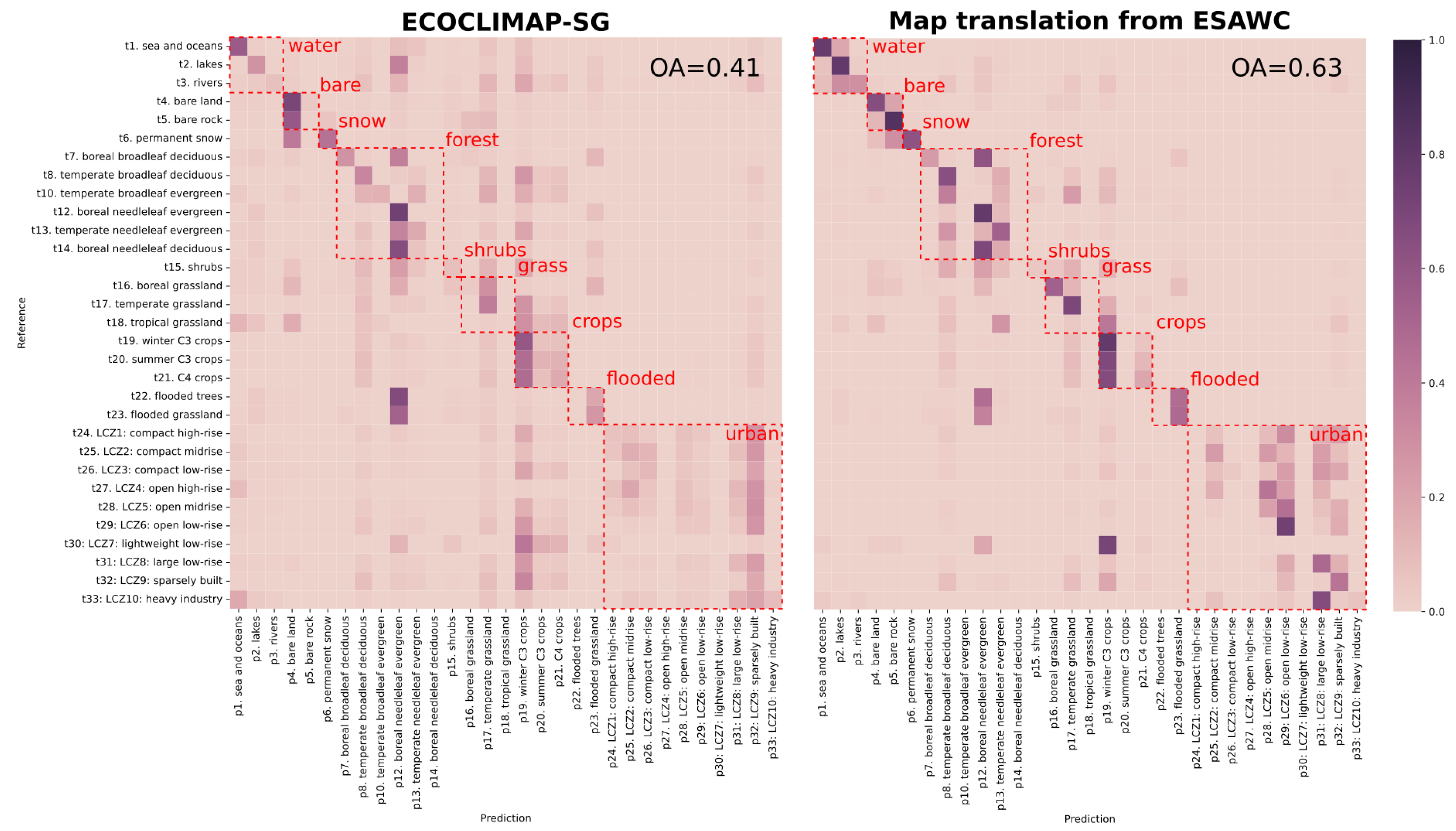
Figure 4.
Recall matrices for (left) ECOSG (right) the inference results. Primary labels are identified in red dashed squares. The reference is ECOSG+ in each case.
Figure 4.
Recall matrices for (left) ECOSG (right) the inference results. Primary labels are identified in red dashed squares. The reference is ECOSG+ in each case.
4.2. Evaluation of ECOSG-ML against LUCAS
Figure 5 was obtained as described in Section 3.5. It shows the evolution of the overall accuracy against LUCAS obtained for different threshold values in the merging process (see Section 3.3). The coloured dashed lines each correspond to a member of ECOSG-ML and they are identified by the value u used in the inversion of the CDF (see Section 3.4, the value None corresponds to the control member). The black solid line corresponds to ECOSG+ when we take different values for the threshold (see Equation (12) in [23]). The black dotted line corresponds to ECOSG (which is flat because it does not depend on any quality threshold).
All members have a better overall accuracy than ECOSG+ and ECOSG for all quality threshold values. It confirms that replacing ECOSG by the inference improves the quality of the map. ECOSG+ and all ECOSG-ML members show a two-stage dependency on the quality thresholds. For thresholds below 0.3, the overall accuracy is stable for ECOSG+ and increases for all ECOSG-ML members as the threshold increases. For thresholds above 0.3, the overall accuracy decreases as the threshold increases. For ECOSG+, this is explained by the direct effect of the threshold: as increases, more pixels will be taken from ECOSG, therefore the score converges to the one of ECOSG. For ECOSG-ML, the overall accuracy decreases as increases, but the rate of decrease is not as high as for ECOSG+ and it is different for each member. This behaviour can be explained by the fact that increasing results in more pixels being taken from the inference. If the inference is out of its application domain (i.e. the diversity criterion is not met), the labels are taken from ECOSG+, which is equal to ECOSG in that case. Therefore, the decrease is explained by the greater proportion of ECOSG pixels as increases, but the decrease is not as high as with ECOSG+ because the inference results, when applicable, improve upon ECOSG. Moreover, the spread of the members logically increases as the number of pixels taken from the inference increases.
The maximum overall accuracy is obtained for all members with . Therefore the maps exported in the archive associated with this paper use this value for the quality threshold. The results provided in the qualitative evaluations were done with the initial value of , as this was used in [23].
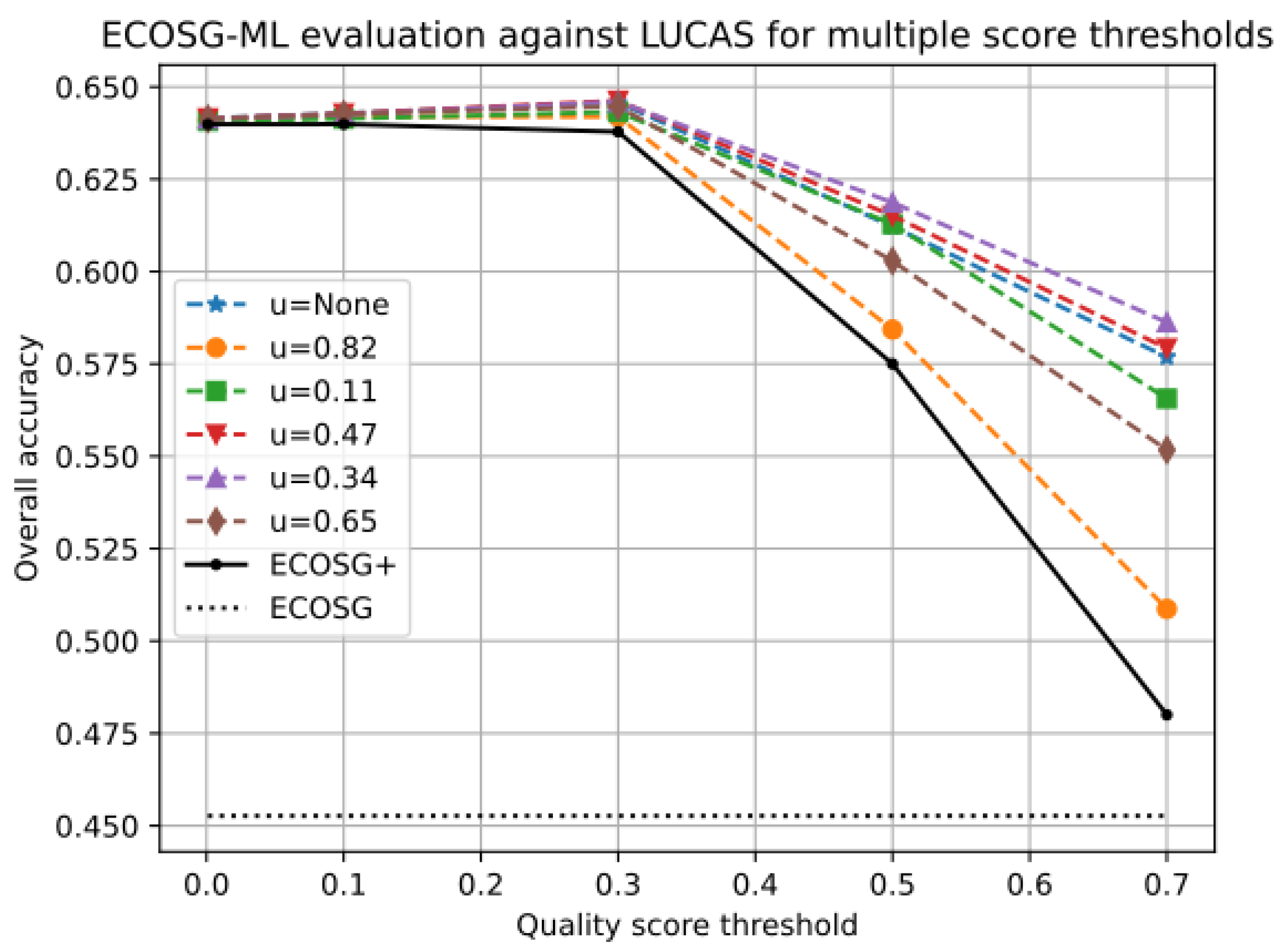
Figure 5.
Overall accuracy with LUCAS as the reference for different threshold values and all ECOSG-ML members.
Figure 5.
Overall accuracy with LUCAS as the reference for different threshold values and all ECOSG-ML members.
4.3. Qualitative Evaluation of the Final Map
Figure 6 shows five geographical areas that exemplify the content of the land cover maps. These are the same areas as in [23]. Each row represents one of these geographical areas and is identified on the left hand side by a toponym, the country it is in, and the longitude-latitude coordinates of the central point. The first row is the Snaefell glacier in Iceland. The second row is centred on Nanterre, France, in the north-western part of the Paris urban area. The third row is the small islands of Kihdinluoto in the south-west of Finland. The fourth row is a rural part of Portugal, around the small town of Pinhel. The fifth and last row is the oasis town of El Menia, in the Sahara desert (Algeria). The geographical areas have been chosen to display a large variety of landscapes and latitudes within the EURAT domain. All patches are 0.0833º in size, which represents approximately 8 km at low latitudes.
Each column represents a different land cover map introduced in Section 2.1. The first column is ESA WorldCover, the source map in the map translation. The second column is ECOSG, currently used in NWP and the baseline to improve upon. The third column is ECOSG+, the target of the map in the map translation. The fourth column is ECOSG-ML, the control member after merging. The fifth and last column is the map of the ECOSG+ quality score, used to select the training and testing patches (see Section 2.2) and to produce the final map (see Section 3.3). The colorbars are given in Figure 1.
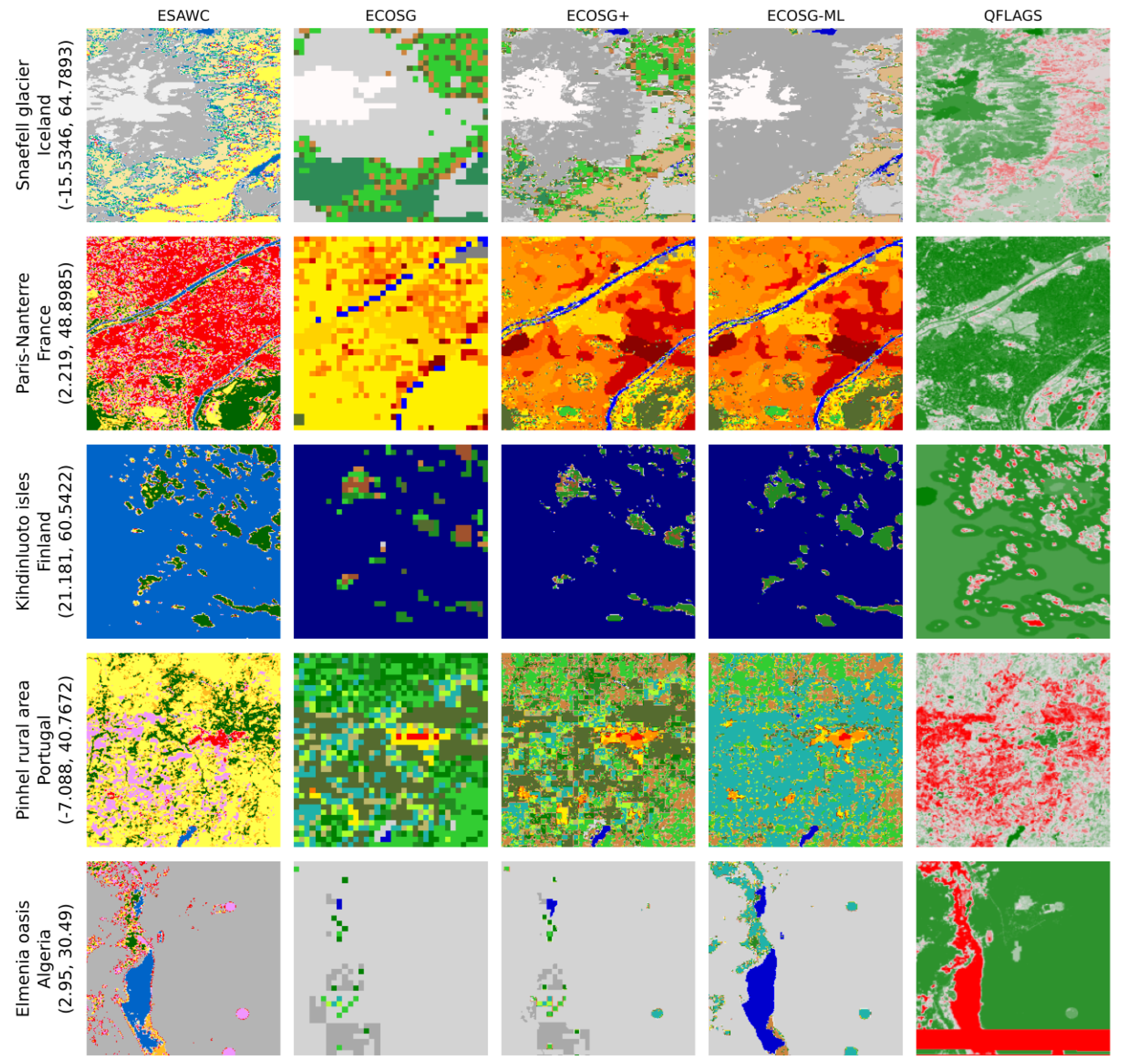
Figure 6.
Examples of patches at various locations (rows) on ESA WorldCover, ECOSG, ECOSG+, ECOSG-ML and the ECOSG+ quality score (columns) maps. All patches are of size 0.0833º in EPSG:4326. The coordinates given on the left hand side are the longitude-latitude coordinates of the central point of each patch. The colorbars are given in Figure 1.
The main focus of this figure is to visualize the qualitative improvement of ECOSG-ML over ECOSG and ECOSG+. The ESA WorldCover and quality score maps are shown for the insight they bring on the map differences. In comparison with ECOSG, ECOSG-ML clearly has a better resolution in each case displayed here. The details that are visible in ECOSG-ML match those in ESA WorldCover, which is satisfying because the resolution of ESA WorldCover (approx. 10 m) is high enough to validate the smallest scales of ECOSG-ML. Note that the improvement in resolution is also very clear between ECOSG and ECOSG+, as already demonstrated in [23]. However, we can still see some low-resolution areas, for example on the eastern edge of the Snaefell glacier (first row), the surroundings of Pinhel (forth row) and almost all of the El Menia area (last row). According to the ECOSG+ map-building methodology, this is the result of discrepancies between the maps that provide data in these areas. Such discrepancies are captured as uncertainty in the land cover and tracked with low quality scores. As a result, the low resolution areas in ECOSG+ match those with low quality scores (red or grey color in the fifth column). When the quality flag is low, and as long as the inference can be applied, we are within the criteria that were outlined in Section 3.3 to use the inference results in ECOSG-ML. Therefore, the differences between ECOSG+ and ECOSG-ML are concentrated on low quality flags areas. One can see that the low resolution areas are replaced by more realistic patterns, which is a qualitative improvement. Moreover, the added details match those visible in ESA WorldCover (e.g. the lake on the south-east of the Snaefell glacier or the lake and town in El Menia).
4.4. Demonstration of Ensemble Land Cover Generation
As described in Section 3.4, the inference provides land cover class probabilities that enable ensemble generation when sampling those probabilities. Figure 7 shows examples of such ensembles. The first two rows are also in Figure 6 (as rows 4 and 5, see text there for description) and the columns show different members. The other rows in Figure 6 have higher quality score, there are only minor differences between the members of the ensemble. Therefore, we choose to show three other location to better illustrate the variability across the different members. The third row is near the town of Iziaslav, surrounded by crop lands in the west of Ukraine. The fourth row is near the town of El Hichria, in central Tunisia. The fifth row shows mountainous terrain near Masmullar, in south of Spain. The first column in Figure 7 is the same as the fourth column in Figure 6 and is obtained by picking the highest probability label for each pixel. The next five columns of Figure 7 are obtained with CDF inversion with the random value u given at the top. The last column shows the ECOSG+ quality score with a transition value at 0.3 (in stead of 0.525 in Figure 6).
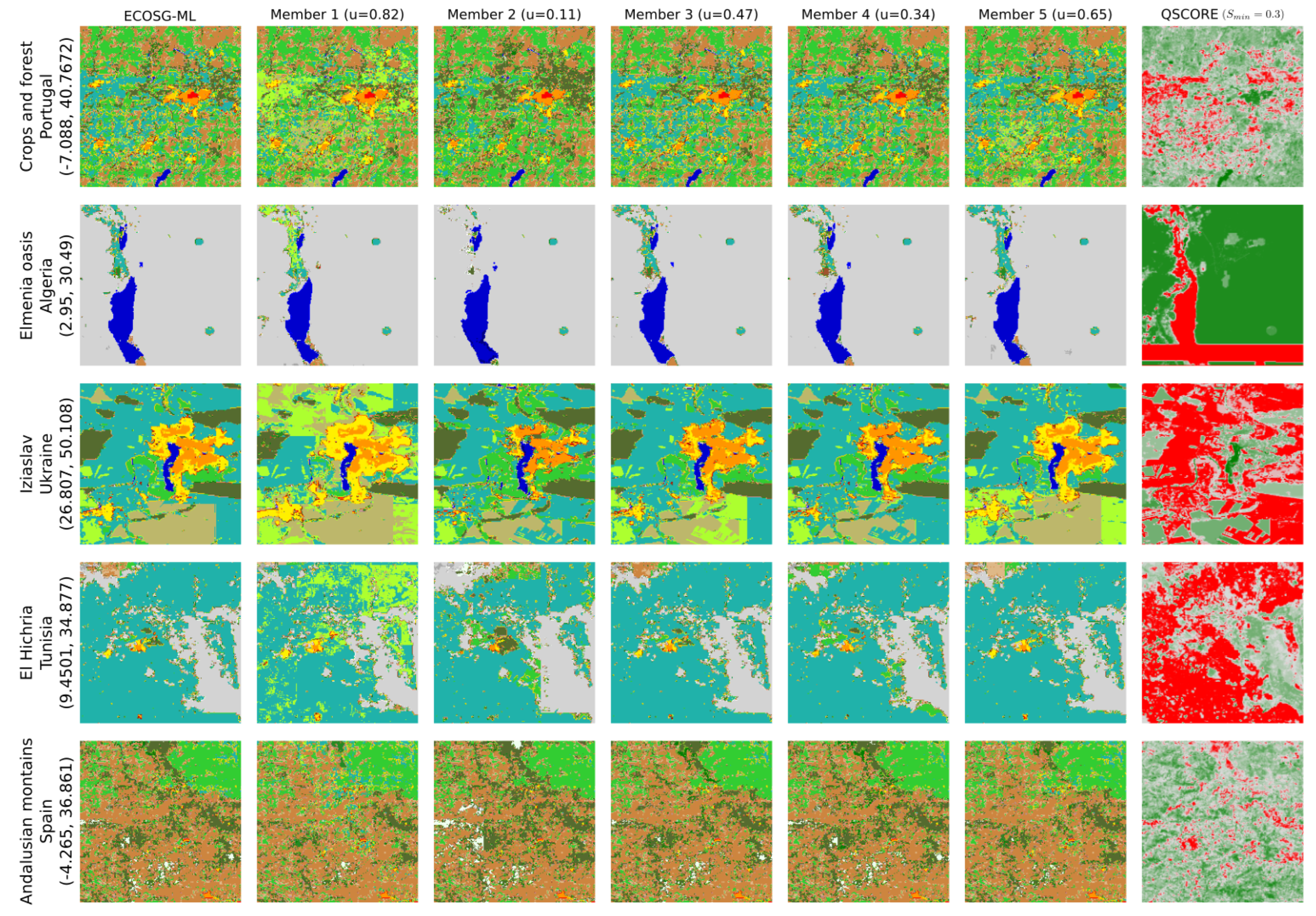
Figure 7.
Example of a land cover ensemble. The patches (rows) are the same as in Figure 6 but the columns show the 5 land cover members derived from the land cover probabilities from the output of the map translation.
Figure 7.
Example of a land cover ensemble. The patches (rows) are the same as in Figure 6 but the columns show the 5 land cover members derived from the land cover probabilities from the output of the map translation.
Globally and qualitatively the generated members look realistic, despite visible discrepancies. According to the ensemble generation methodology, the discrepancies concentrate on where the ECOSG+ quality score is low. Following the outcome of the comparison with LUCAS, the quality score threshold is set to 0.3 (red in the 6th column means below 0.3, green means above). Therefore, the high quality features are equal across all members (e.g. the desert and crops circles in Elmenia, the town of Pinhel, the lake of Iziaslav). Some features are also common to all members despite having very low quality scores (e.g. the lake in Elmenia), which means that the inference output gives a very high probability on the given labels. Some other features are noticeably different from one member to another (e.g. the type of crop around Iziaslav, the extension of the town of Pinhel, the type of soil in El Hichria), which shows that other labels have significant probability, although it is not maximum. In some examples, artificially straight transitions are visible (e.g. in Iziaslav). These are the results of the patch-wise construction of ECOSG-ML for running the inference.
These examples show that it is possible to generate ensemble land cover maps with inference output. This could lead to an additional way of accounting for the uncertainty in land cover in the weather forecast. However, these examples only provide a qualitative evaluation of the generated ensemble. Further studies are necessary to quantitatively assess how representative of the uncertainty on the land cover the ensemble is.
5. Discussion
This section includes a critical discussion on the results and emphasizes known limitations to help with future improvements of the map.
5.1. Limitations
This section focuses on the known limitations of the ECOSG-ML dataset. These are summarized in three categories:
- Obviously wrong classifications. Some pixels may show inconsistent land cover (e.g. lake or river pixels surrounded by sea pixels, or permanent snow at low altitude or latitude).
- Default secondary labels. For some primary labels (e.g. “Crops” or “Forest”), a default secondary label is predicted almost all the time (“19. winter C3 crops” for “Crops”, “8. temperate broadleaf deciduous” or “12. boreal needleleaf evergreen” for “Forest”), as visible in Figure 4. This results in correct primary label classification but incorrect secondary label classification.
- Too simple ensemble construction. With the current method of generating the members, u is the same everywhere on the map. As a result, all locations are modified in the same way, as if the uncertainty varies the same way everywhere, which may not be valid. Moreover, only a qualitative evaluation of the ensemble is made here. In particular, the representativity of the ensemble to the land cover uncertainty is not established.
5.2. Potential Directions for Improvement
This section discusses steps that could be taken to improve the ECOSG-ML land cover maps. These steps mainly suggest solutions to the limitations identified in the previous section.
- Enrich input information. Many of the current limitations are due to a lack of input information. The addition of informative variables like elevation or a position encoding would certainly help the network to better detect some labels (such as “6. permanent snow” or the bioclimatic classification). Such complementary information can be added as input to the auto-encoder or in the latent space (therefore as input to the decoder). For example, despite the limitations of ECOSG, it certainly contains valuable information to distinguish some secondary labels. After being projected in the latent space, the information from any land cover has the same resolution and channels, which makes the combination easier.
- Better loss function. The current loss is unaware of class similarities (classes are more similar within the same primary label, for example) and is unweighted. It is possible to put more weight on the loss of some classes, if these classes are critical, or to compensate for an unbalanced training set.
- Better input for CDF inversion. In this work, we used a single random number for all pixels and patches. This is better than to make a random draw for each pixel because the latter reduces correlation with geographical proximity, and is technically very simple. However, this is not entirely satisfactory because all locations are modified in the same way. A suggestion for future developments is to use a 2-dimensional stochastic process with appropriate properties to generate the members.
Alternative encoder and decoder architectures were also tested during the creation of ECOSG-ML. We tried symmetric architectures for the encoder and the decoder with a mix of convolutional and attention layers and we tried to reduce the resolution of the latent space. The results were marginally better (overall accuracy of 0.64 against ECOSG+) with attention layers and a 200×200 latent space, but qualitatively not as satisfying, with smoother landscape features compared to the original architecture. Our impression at that stage is that improving the input data gives better results than improving the ML method. However, the tests we did with alternative ML methods are clearly not sufficient to support such a claim. The tested architectures are openly shared along with the rest of the code.
5.3. Prospects for Future Use
This section gives prospects for further use of the ECOSG-ML maps, regardless of the limitations and potential improvements discussed in the previous sections.
- Update other components of physiography. To be used in NWP the whole physiography database must be updated to be consistent with the land cover maps. Other components include Leaf Area Index (LAI), albedo, lakes parameters and tree height. In ECOSG, these components are present but stored in a way that is highly dependent on the land cover map (LAI and tree height only stored for pixels with vegetation or trees etc.). Therefore, despite a priori compatibility as ECOSG is already used in NWP, it can be complicated to reuse the values of ECOSG. Moveover, the values for the other components might be outdated since ECOSG is a static database. Consequently, we recommend to use up-to-date high-quality sources for these other components as much as possible. Over Europe, Copernicus products345 are available. Machine learning can also help to provide up-to-date and fit-for-purpose datasets for these components, such as in e.g., [30].
- Assess benefit of new maps in NWP. Once an updated physiography database is available, the potential benefit of this update will need to be evaluated. In particular, the resolution of ECOSG-ML also allows sub-kilometer NWP experiments to be carried out, for which the influence of the physiography is expected to be large.
- Assess benefit of ensemble land cover maps in physics-driven and data-driven ensemble forecasts. Besides the remaining questions about the representativity of the ensemble, there are open questions on the opportunities for using ensemble land covers in EPS. The effect of using a different land cover for each forecast member is unknown and is, in our opinion, an interesting question.
6. Conclusions
This article describes the ECOCLIMAP-SG-ML dataset, which builds upon the ECOCLIMAP-SG+ dataset, presented in a companion article. To produce the ECOCLIMAP-SG-ML dataset we leverage the quality score provided with the ECOCLIMAP-SG+ dataset and map translation with AI. The AI translates ESA WorldCover v200 to ECOSG+ with convolutional auto-encoders, and provides a probability distribution of land cover labels which is exploited to create an ensemble of six land cover maps. The AI is first evaluated alone against a high-quality subset of ECOSG+. Then the final map, which is a composite of ECOSG+ and the AI inference, is evaluated against LUCAS.
The inference alone has better F1-scores than ECOCLIMAP-SG for all primary labels and 24 of the 33 secondary labels. The overall accuracy of the inference is estimated to be 0.63, while that for ECOCLIMAP-SG is estimated to be 0.41. Therefore the inference outperforms ECOCLIMAP-SG when compared to the testing subset of ECOSG+. The comparison to LUCAS shows that all members of ECOCLIMAP-SG-ML have a better overall accuracy than ECOCLIMAP-SG and ECOCLIMAP-SG+, for all quality score thresholds. The quality threshold in Equation (1) is set to 0.3 because it gives the maximum overall accuracy against LUCAS. The qualitative evaluation of ECOCLIMAP-SG-ML on a limited set of patches is also satisfying, for the control member compared to ECOCLIMAP-SG and ECOCLIMAP-SG+, and for the ensemble variability.
However, several limitations have been identified, such as default secondary labels for some primary labels, obvious misclassifications and unchecked representativity of the ensemble. We suspect these limitations are mainly due to the information provided to the AI, which can be extended in future work by including elevation and/or position encoding. The latent space of the auto-encoders allows for the possibility to include information from multiple land cover maps. Finally, the next step to make use of ECOCLIMAP-SG-ML in NWP is to update the other components of the physiography database, and to assess the benefits of both the higher resolution and the ensemble component.
Author Contributions
Conceptualization, methodology, investigation, software and writing—original draft preparation, T.R.; validation and data curation, T.R. and G.B.; writing—review and editing, T.R., G.B and E.G.; supervision, E.G. All authors have read and agreed to the published version of the manuscript.
Funding
This research received no external funding.
Data Availability Statement
The ECOSG-ML data is available on Zenodo at this link: https://doi.org/10.5281/zenodo.11242910 The archive contains:
- The 6 land cover maps described in this paper (users who do not need the ensemble may download member 0 only), each of these stored as 200 TIF files.
- The weights obtained after training, stored in Pytorch checkpoint (to be loaded with the provided code).
- The DS1 and DS2 datasets used fort raining and testing, stored as HDF5 files
The code used to create ECOSG-MLand to produce the results shown in this document is accessible at this link:https://github.com/ThomasRieutord/MT-MLULC
Acknowledgments
We would like to thank Luc Baudoux for sharing his work openly and under a permissive licence. Our thanks also go to Ekaterina Kurzeneva (Finnish Meteorological Institute) for her initiative on this topic and more generally to our colleagues from the ACCORD consortium for their support and fruitful discussions.
Conflicts of Interest
The authors declare no conflicts of interest.
Abbreviations
The following abbreviations are used in this manuscript:
| DS1 | Dataset for phase 1 of the training (France mainland, 5 maps) |
| DS2 | Dataset for phase 2 of the training (EURAT, 3 maps) |
| ECOSG | ECOCLIMAP-SG: a physiography database currently used in NWP |
| ECOSG+ | ECOCLIMAP-SG+: the land cover map created by [23], used as a reference |
| ECOSG-ML | ECOCLIMAP-SG-ML: the ensemble land cover map described in this manuscript |
| EPS | Ensemble Prediction Systems |
| EURAT | Europe-Atlantic domain (longitudes: -32 to 42, latitudes: 20 to 72) |
| NWP | Numerical Weather Prediction |
References
- Bauer, P.; Thorpe, A.; Brunet, G. The quiet revolution of numerical weather prediction. Nature 2015, 525, 47–55. [Google Scholar] [CrossRef] [PubMed]
- Nuissier, O.; Duffourg, F.; Martinet, M.; Ducrocq, V.; Lac, C. Hectometric-scale simulations of a Mediterranean heavy-precipitation event during the Hydrological cycle in the Mediterranean Experiment (HyMeX) first Special Observation Period (SOP1). Atmospheric Chemistry and Physics 2020, 20, 14649–14667. [Google Scholar] [CrossRef]
- Sabatier, T.; Largeron, Y.; Paci, A.; Lac, C.; Rodier, Q.; Canut, G.; Masson, V. Semi-idealized simulations of wintertime flows and pollutant transport in an Alpine valley. Part II: Passive tracer tracking. Quarterly Journal of the Royal Meteorological Society 2020, 146, 827–845. [Google Scholar] [CrossRef]
- Lemonsu, A.; Alessandrini, J.; Capo, J.; Claeys, M.; Cordeau, E.; de Munck, C.; Dahech, S.; Dupont, J.; Dugay, F.; Dupuis, V. ; others. The heat and health in cities (H2C) project to support the prevention of extreme heat in cities, 2024.
- Seity, Y.; Brousseau, P.; Malardel, S.; Hello, G.; Bénard, P.; Bouttier, F.; Lac, C.; Masson, V. The AROME-France Convective-Scale Operational Model. Monthly Weather Review 2011, 139, 976–991. [Google Scholar] [CrossRef]
- Bengtsson, L.; Andrae, U.; Aspelien, T.; Batrak, Y.; Calvo, J.; Rooy, W.d.; Gleeson, E.; Hansen-Sass, B.; Homleid, M.; Hortal, M.; Ivarsson, K.I.; Lenderink, G.; Niemelä, S.; Nielsen, K.P.; Onvlee, J.; Rontu, L.; Samuelsson, P.; Muñoz, D.S.; Subias, A.; Tijm, S.; Toll, V.; Yang, X.; Køltzow, M.Ø. The HARMONIE–AROME Model Configuration in the ALADIN–HIRLAM NWP System. Monthly Weather Review 2017, 145, 1919–1935. [Google Scholar] [CrossRef]
- Masson, V.; Le Moigne, P.; Martin, E.; Faroux, S.; Alias, A.; Alkama, R.; Belamari, S.; Barbu, A.; Boone, A.; Bouyssel, F.; Brousseau, P.; Brun, E.; Calvet, J.C.; Carrer, D.; Decharme, B.; Delire, C.; Donier, S.; Essaouini, K.; Gibelin, A.L.; Giordani, H.; Habets, F.; Jidane, M.; Kerdraon, G.; Kourzeneva, E.; Lafaysse, M.; Lafont, S.; Lebeaupin Brossier, C.; Lemonsu, A.; Mahfouf, J.F.; Marguinaud, P.; Mokhtari, M.; Morin, S.; Pigeon, G.; Salgado, R.; Seity, Y.; Taillefer, F.; Tanguy, G.; Tulet, P.; Vincendon, B.; Vionnet, V.; Voldoire, A. The SURFEXv7.2 land and ocean surface platform for coupled or offline simulation of earth surface variables and fluxes. Geoscientific Model Development 2013, 6, 929–960. [Google Scholar] [CrossRef]
- Le Moigne, P.; Boone, A.; Calvet, J.C.; Decharme, B.; Faroux, S.; Gibelin, A.L.; Lebeaupin, C.; Mahfouf, J.F.; Martin, E.; Masson, V. SURFEX scientific documentation. Note de centre (CNRM/GMME), Météo-France, Toulouse, France 2009, 268. [Google Scholar]
- Zanaga, D.; Van De Kerchove, R.; Daems, D.; De Keersmaecker, W.; Brockmann, C.; Kirches, G.; Wevers, J.; Cartus, O.; Santoro, M.; Fritz, S.; Lesiv, M.; Herold, M.; Tsendbazar, N.; Xu, P.; Ramoino, F.; Arino, O. ESA WorldCover 10 m 2021 v200. 2022. [Google Scholar] [CrossRef]
- Malinowski, R.; Lewiński, S.; Rybicki, M.; Gromny, E.; Jenerowicz, M.; Krupiński, M.; Nowakowski, A.; Wojtkowski, C.; Krupiński, M.; Krätzschmar, E.; Schauer, P. Automated Production of a Land Cover/Use Map of Europe Based on Sentinel-2 Imagery. Remote Sensing 2020, 12, 3523. [Google Scholar] [CrossRef]
- Venter, Z.S.; Sydenham, M.A.K. Continental-Scale Land Cover Mapping at 10 m Resolution Over Europe (ELC10). Remote Sensing 2021, 13, 2301. [Google Scholar] [CrossRef]
- Mirmazloumi, S.M.; Kakooei, M.; Mohseni, F.; Ghorbanian, A.; Amani, M.; Crosetto, M.; Monserrat, O. ELULC-10, a 10 m European Land Use and Land Cover Map Using Sentinel and Landsat Data in Google Earth Engine. Remote Sensing 2022, 14, 3041. [Google Scholar] [CrossRef]
- Sumbul, G.; de Wall, A.; Kreuziger, T.; Marcelino, F.; Costa, H.; Benevides, P.; Caetano, M.; Demir, B.; Markl, V. BigEarthNet-MM: A Large Scale Multi-Modal Multi-Label Benchmark Archive for Remote Sensing Image Classification and Retrieval. IEEE Geoscience and Remote Sensing Magazine 2021, 9, 174–180. [Google Scholar] [CrossRef]
- Schmitt, M.; Hughes, L.H.; Qiu, C.; Zhu, X.X. SEN12MS – A Curated Dataset of Georeferenced Multi-Spectral Sentinel-1/2 Imagery for Deep Learning and Data Fusion, 2019. arXiv:1906.07789 [cs].
- Zhang, D.; Zhao, J.; Chen, J.; Zhou, Y.; Shi, B.; Yao, R. Edge-aware and spectral–spatial information aggregation network for multispectral image semantic segmentation. Engineering Applications of Artificial Intelligence 2022, 114, 105070. [Google Scholar] [CrossRef]
- Aksoy, A.K.; Ravanbakhsh, M.; Kreuziger, T.; Demir, B. A Consensual Collaborative Learning Method for Remote Sensing Image Classification Under Noisy Multi-Labels. 2021 IEEE International Conference on Image Processing (ICIP), 2021, pp. 3842–3846. ISSN: 2381-8549. [CrossRef]
- Baudoux, L.; Inglada, J.; Mallet, C. Toward a Yearly Country-Scale CORINE Land-Cover Map without Using Images: A Map Translation Approach. Remote Sensing 2021, 13, 1060. [Google Scholar] [CrossRef]
- Baudoux, L.; Inglada, J.; Mallet, C. Multi-nomenclature, multi-resolution joint translation: an application to land-cover mapping. International Journal of Geographical Information Science 2023, 37, 403–437. [Google Scholar] [CrossRef]
- Gneiting, T.; Raftery, A.E. Weather forecasting with ensemble methods. Science 2005, 310, 248–249. [Google Scholar] [CrossRef] [PubMed]
- Frogner, I.L.; Andrae, U.; Bojarova, J.; Callado, A.; Escribà, P.; Feddersen, H.; Hally, A.; Kauhanen, J.; Randriamampianina, R.; Singleton, A.; others. HarmonEPS—the HARMONIE ensemble prediction system. Weather and Forecasting 2019, 34, 1909–1937. [Google Scholar] [CrossRef]
- Ben Bouallègue, Z.; Clare, M.C.; Magnusson, L.; Gascon, E.; Maier-Gerber, M.; Janoušek, M.; Rodwell, M.; Pinault, F.; Dramsch, J.S.; Lang, S.T. ; others. The rise of data-driven weather forecasting: A first statistical assessment of machine learning-based weather forecasts in an operational-like context. Bulletin of the American Meteorological Society, 2024. [Google Scholar]
- Oskarsson, J.; Landelius, T.; Lindsten, F. Graph-based neural weather prediction for limited area modeling. arXiv preprint arXiv:2309.17370, 2023. [Google Scholar]
- Bessardon, G.; Rieutord, T.; Gleeson, E.; Palmason, B.; Oswald, S. High-resolution land use land cover dataset for meteorological modelling – Part 1: ECOCLIMAP-SG+ an agreement-based dataset. Land 2024. [Google Scholar]
- Venter, Z.S.; Barton, D.N.; Chakraborty, T.; Simensen, T.; Singh, G. Global 10 m land use land cover datasets: A comparison of dynamic world, world cover and esri land cover. Remote Sensing 2022, 14, 4101. [Google Scholar] [CrossRef]
- Inglada, J.; Vincent, A.; Arias, M.; Tardy, B.; Morin, D.; Rodes, I. Operational High Resolution Land Cover Map Production at the Country Scale Using Satellite Image Time Series. Remote Sensing 2017, 9, 95. [Google Scholar] [CrossRef]
- EEA. CORINE Land Cover 2018 (vector), Europe, 6-yearly - version 2020_20u1, May 2020, 2018. [CrossRef]
- Ballin, M.; Barcaroli, G.; Masselli, G. New LUCAS 2022 sample and subsamples design: Criticalities and solutions. Technical report, Publications Office of the European Union, 2022. [CrossRef]
- Devroye, L. Non-Uniform Random Variate Generation; Springer: New York, NY, 1986. [Google Scholar] [CrossRef]
- Fawcett, T. An introduction to ROC analysis. Pattern recognition letters 2006, 27, 861–874. [Google Scholar] [CrossRef]
- Keany, E.; Bessardon, G.; Gleeson, E. Using machine learning to produce a cost-effective national building height map of Ireland to categorise local climate zones. Advances in Science and Research. Copernicus GmbH, 2022, Vol. 19, pp. 13–27. [CrossRef]
| 1 | The ECOCLIMAP-SG wiki: https://opensource.umr-cnrm.fr/projects/ecoclimap-sg/wiki (last access: 2024/10/15 11:15:12) |
| 2 | Zenodo archive: https://doi.org/10.5281/zenodo.5843595 (last accessed 2024/10/15 11:15:12) |
| 3 | Leaf area index: https://land.copernicus.eu/en/products/vegetation/high-resolution-leaf-area-index (last accessed 2024/10/15 11:15:12) |
| 4 | Albedo: https://www.copernicus.eu/en/global-land-surface-albedo (last accessed 2024/10/15 11:15:12) |
| 5 | Building height: https://land.copernicus.eu/api/en/products/urban-atlas/building-height-2012 (last accessed 2024/10/15 11:15:12) |
Figure 1.
Set of labels and colormaps of land cover labels for ESA WorldCover, ECOCLIMAP-SG (primary and secondary) and ECOSG+ quality score.
Figure 1.
Set of labels and colormaps of land cover labels for ESA WorldCover, ECOCLIMAP-SG (primary and secondary) and ECOSG+ quality score.
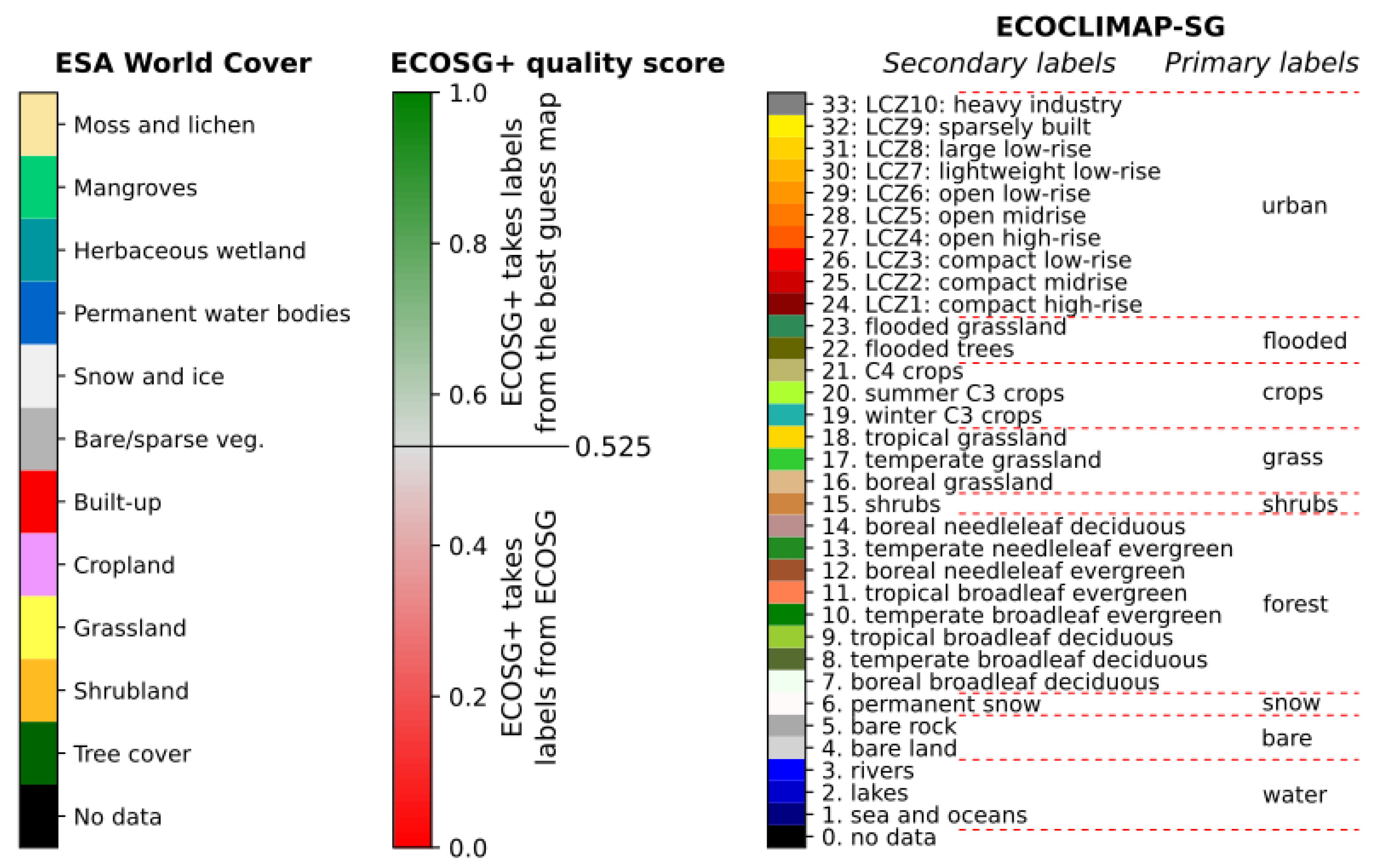
Figure 2.
Locations of the 5000 patches in the DS2 dataset on the EURAT domain (a), and illustration of the splitting procedure (b).
Figure 2.
Locations of the 5000 patches in the DS2 dataset on the EURAT domain (a), and illustration of the splitting procedure (b).
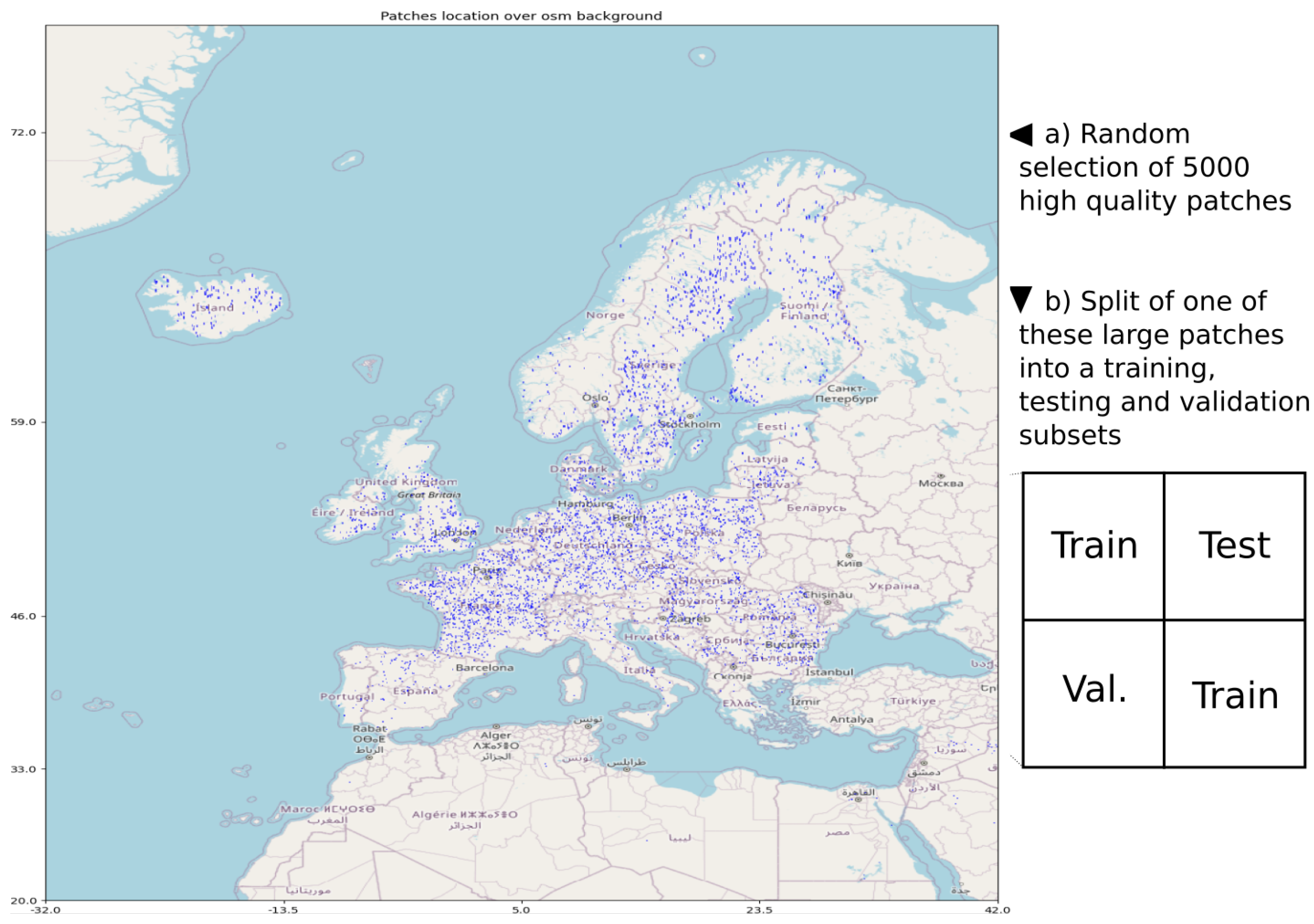
Figure 3.
Illustration of the map translation method. The top row represents the same geographical region in Map 1 and Map 2. The size of the square accounts for the resolution (Map 1 has a higher resolution than Map 2) and the number of stacked squares accounts for the number of labels (Map 1 has less labels than Map 2). The translation from Map 1 to Map 2 is made with auto-encoders sharing the same latent space. The translation is performed by using the encoder from Map 1 and the translator to Map 2. These auto-encoders are trained to minimize the loss with the three components shown in the figure.
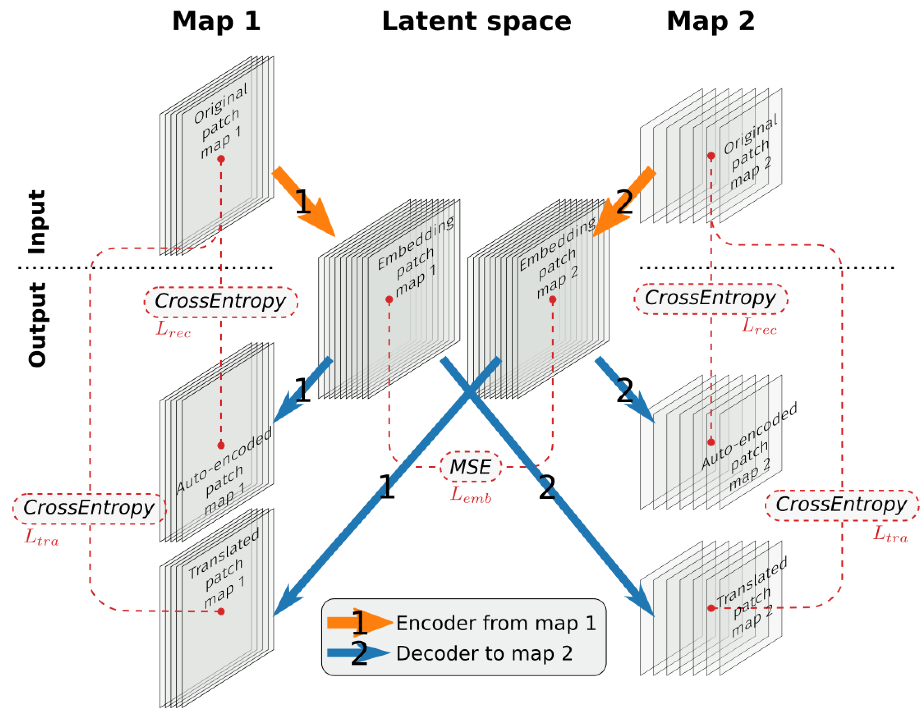

Table 1.
F1-scores for each primary and secondary label. The best score for each line is highlighted in bold font. The rightmost column shows the support for each label: when it is lower than 1% the total number of pixels is shown, otherwise the percentage is shown (with %). For some labels, not present in the testing set (support is 0) or never predicted, the score is undefined (dash).
| Primary label | Inference | ECOSG | Secondary label | Inference | ECOSG | Support |
|---|---|---|---|---|---|---|
| Water | 0.9149 | 0.4402 | 1. sea and oceans | 0.8185 | 0.5937 | 2% |
| 2. lakes | 0.7615 | 0.305 | 3% | |||
| 3. rivers | 0.3268 | 0.0812 | 140570 | |||
| Bare | 0.8767 | 0.6892 | 4. bare land | 0.645 | 0.4758 | 1% |
| 5. bare rock | 0.7874 | 0.0242 | 1% | |||
| Snow | 0.7018 | 0.4119 | 6. permanent snow | 0.7018 | 0.4119 | 83305 |
| Forest | 0.8806 | 0.6206 | 7. boreal broadleaf deciduous | 0.311 | 0.3506 | 397158 |
| 8. temperate broadleaf deciduous | 0.6397 | 0.4017 | 14% | |||
| 9. tropical broadleaf deciduous | - | - | 0 | |||
| 10. temperate broadleaf evergreen | 0.016 | 0.0808 | 25087 | |||
| 11. tropical broadleaf evergreen | - | - | 0 | |||
| 12. boreal needleleaf evergreen | 0.7628 | 0.6183 | 12% | |||
| 13. temperate needleleaf evergreen | 0.5098 | 0.2372 | 7% | |||
| 14. boreal needleleaf deciduous | - | - | 41558 | |||
| Shrubs | 0.0855 | 0.0509 | 15. shrubs | 0.0855 | 0.0509 | 228646 |
| Grass | 0.6983 | 0.428 | 16. boreal grassland | 0.5956 | 0.0574 | 1% |
| 17. temperate grassland | 0.6848 | 0.4222 | 10% | |||
| 18. tropical grassland | - | 0.0072 | 597 | |||
| Crops | 0.8513 | 0.6773 | 19. winter C3 crops | 0.7021 | 0.5265 | 25% |
| 20. summer C3 crops | 0.0 | 0.1015 | 3% | |||
| 21. C4 crops | 0.2624 | 0.1984 | 8% | |||
| Flooded | 0.5621 | 0.2335 | 22. flooded trees | 0.0118 | - | 53089 |
| 23. flooded grassland | 0.5478 | 0.2293 | 1% | |||
| Urban | 0.7543 | 0.3387 | 24. LCZ1: compact high-rise | - | 0.0284 | 8955 |
| 25. LCZ2: compact midrise | 0.3257 | 0.1207 | 53105 | |||
| 26. LCZ3: compact low-rise | 0.0697 | 0.0683 | 33709 | |||
| 27. LCZ4: open high-rise | 0.0272 | - | 9746 | |||
| 28. LCZ5: open midrise | 0.282 | 0.0676 | 139875 | |||
| 29: LCZ6: open low-rise | 0.6833 | 0.0781 | 1% | |||
| 30: LCZ7: lightweight low-rise | - | - | 38 | |||
| 31: LCZ8: large low-rise | 0.4995 | 0.103 | 254488 | |||
| 32: LCZ9: sparsely built | 0.434 | 0.1319 | 3% | |||
| 33: LCZ10: heavy industry | 0.0998 | 0.0881 | 10641 | |||
| Overall accuracy | 0.831 | 0.583 | Overall accuracy | 0.634 | 0.411 | 50M |
Disclaimer/Publisher’s Note: The statements, opinions and data contained in all publications are solely those of the individual author(s) and contributor(s) and not of MDPI and/or the editor(s). MDPI and/or the editor(s) disclaim responsibility for any injury to people or property resulting from any ideas, methods, instructions or products referred to in the content. |
© 2024 by the authors. Licensee MDPI, Basel, Switzerland. This article is an open access article distributed under the terms and conditions of the Creative Commons Attribution (CC BY) license (http://creativecommons.org/licenses/by/4.0/).
Copyright: This open access article is published under a Creative Commons CC BY 4.0 license, which permit the free download, distribution, and reuse, provided that the author and preprint are cited in any reuse.


