
Submitted:
09 September 2024
Posted:
09 September 2024
You are already at the latest version
Abstract
Machine learning methods used for classification can face challenges due to class imbalance, where a certain class is underrepresented. Over/under-sampling of minority/majority class observations, or model selection for ensemble methods alone, may not be effective if the class imbalance ratio is very high. To address this issue, this paper proposes a method called enhance tree ensemble (ETE) based on generating synthetic data for minority class observations in conjunction with tree selection based on their performance on the training data. The proposed method first generates minority class instances to balance the training data and then uses the idea of tree selection by leveraging out-of-bag (〖ETE〗_OOB) and sub-samples (〖ETE〗_SS) observations, respectively. The efficacy of the proposed method is assessed using twenty benchmark problems for binary classification with moderate to extreme class imbalance, comparing it against other well-known methods such as optimal tree ensemble (OTE), SMOTE random forest (〖RF〗_SMOTE), over-sampling random forest (〖RF〗_OS), under-sampling random forest (〖RF〗_US), k-nearest-neighbor (k-NN), support vector machine (SVM), tree, and artificial neural network (ANN). Performance metrics such as classification error rate and precision are used for evaluation purposes. The analyses of the study revealed that the proposed method, based on data balancing and model selection, yielded better results than the other methods.
Keywords:
Random Forest
; Tree Selection
; Classification
; Class-Imbalance Problem
; Synthetic Data Generation
MSC: 68U01; 62P10; 62P20
1. Introduction
The challenge of dealing with imbalanced problems in the field of machine learning has been a significant topic for a long time. Imbalanced problems, which have an uneven distribution of classes, can lead to biased and subpar results, affecting the accuracy of classification models. To tackle this issue, researchers have developed various methods, including sampling methods and specialized algorithms [1,2,3,4]. Oversampling techniques such as extreme anomalous oversampling technique (EXOT) [5], which synthesizes positive instances based on anomalous scores is an example of such methods. Another strategy involves increasing minority samples while maintaining low misclassification rates for the majority class [6]. Additionally, imbalanced problems can be tackled using re-sampling algorithms such as spread sub-sample, Class Balancer, SMOTE, and Resample [7]. However, the effectiveness of different sampling procedures may vary depending on the specific dataset and the nature of the problem [8,9]. In the context of cancer diagnosis, imbalanced problem is often encountered, and balancing techniques have shown significant improvements in classifier performance. It's crucial to utilize customized approaches because different cancer datasets respond differently to various balancing strategies and classifiers [10].
The performance of machine learning classifiers can be negatively impacted when working with imbalanced problems. The distribution of the training data greatly affects their performance [11]. In a study conducted by [12], several techniques for dealing with class imbalance, including the Synthetic Minority Oversampling Technique (SMOTE) in conjunction with Tomek links and Wilson’s Edited Nearest Neighbor Rule (ENN), were introduced for balancing datasets. However, a systematic comparison of these techniques with optimal tree forest classifiers is currently lacking in the available literature. Similarly, studies in [13,14] have assessed the performance of individual classifiers, such as One Class SVM, Cost-Sensitive SVM, Optimum Path Forest, and decision tree classifier (C4.5 Tree), in the context of imbalanced data.
The study by [15] investigates ensemble techniques, such as the random forest classifier and over-sampling methods, to address class imbalance. Moreover, the study given in [16] addresses the effects of class imbalance on forest point cloud data using a weighted random forest classifier. Most studies suggest that oversampling techniques outperform under-sampling techniques based on assessments made via area under the ROC curve (AUC). While some research [17,18] suggest that oversampling may not always impact performance, it is noted that more complex decision trees can be generated through oversampling. Specialized tree construction methods, such as minority condensation trees, have been proposed to enhance the performance of Random Forest in imbalanced environments [19]. Additionally, incorporating resampling techniques can improve the efficiency of ensemble methods like Random Forests, although these improvements may not always be statistically significant [20]. It has been shown that combining algorithmic strategies with resampling techniques can produce good results [21]. While the choice of splitting indices (GINI index or information gain) does not seem to impact accuracy for balanced or imbalanced data [22], other methods have shown enhanced results. For example, balanced bagging, an ensemble technique, improves the geometric mean, AUC scores, and accuracy of decision tree classification for imbalanced problems [23]. Additionally, using hybrid sampling, which combines techniques like random oversampling and under-sampling, can create balanced datasets that enhance the performance of C4.5 decision trees on imbalanced problems [24]. While there hasn't been a thorough investigation into the most effective combination of the implementation of decision tree and random forest classifiers with hyper-parameter tuning and resampling techniques, there hasn't been a thorough investigation into the most effective combination of these elements in the presence of extreme class imbalances [25].
The concept of optimal tree ensembles (OTE) has become popular in machine learning due to their ability to improve predictive performance and model robustness. Among the various techniques used, out-of-bag (OOB) samples and sub-sampling are crucial for optimizing tree ensembles. Many research papers [26,27] explore the effectiveness of using balanced data and optimal tree forest methods, specifically by utilizing OOB estimates and sub-sampling. In their paper, [28] introduces an improved random forest algorithm that assigns weights to decision trees based on OOB errors. OOB errors can be utilized to estimate the model's performance without needing a separate validation set [29]. The use of OOB observations in modified tree selection techniques for optimal trees ensemble (OTE) is examined by [30] who propose that using OOB observations can improve predictive accuracy for individual and group performance evaluations. Similarly, [31,32] discuss the Modified Balanced Random Forest (MBRF) algorithm, which employs under-sampling based on clustering techniques. This approach differs from the OOB and sub-sampling methods mentioned earlier. To tackle imbalanced data, [33,34,35] propose a random forest algorithm based on Generative Adversarial Networks (GANs), presenting a unique alternative to OOB and sub-sampling. Furthermore, [36] combines the skew-insensitivity of Hellinger distance decision trees with the diversity of Random Forest and Rotation Forest, providing another perspective for optimizing tree-based methods for imbalanced data. In conclusion, the literature suggests that OOB estimates and sub-sampling are valuable techniques in the context of balanced data and optimal tree forests, and can enhance the performance of tree-based models, especially when dealing with imbalanced datasets.
To this end, addressing extreme class imbalance in datasets can be effectively achieved through the use of ensemble tree-based classifiers like Random Forests, potentially enhanced by resampling methods or specialized tree construction techniques. The best approach may differ depending on the specific dataset and context, but a combination of algorithmic and data-level interventions seems to be a promising strategy for improving classifier performance in the presence of class imbalances.
Random forest [37,38], provided an upper bound for the overall prediction error as a function of the accuracy and diversity of the base tree models: i.e.,
where is the total prediction error of the forest, is the estimate of anytree in the forest, and is the weighted correlation between the residuals from two independent classification trees expressed as the mean correlation over the entire random forest. Therefore, developing a tree ensemble that ensures the accuracy and diversity of the base model is believed to yield promising results. Therefore, this study proposes an ensemble method that uses the above concepts to learn effectively from datasets with class-imbalanced problems. First, the given training data is balanced by generating new synthetic observations for the minority class. Consequently, datasets with extreme class imbalances are considered in this study. These data sets are obtained from several publicly available sources. Once the dataset is balanced, classification trees are grown on bootstrap/sub-samples from the data. The training prediction accuracy of each tree is estimated, and the top-performing trees are selected for the final ensemble. Based on the above notion, this study attempted to increase the accuracy of individual tree models in forests, in addition to randomizing their construction. The accuracy is increased by balancing the given training data with the model selection based on individual prediction performance.
The main contributions of this paper are:
- Mitigating the impact of extreme class imbalance on the random forest ensemble.
- Generating synthetic data from the minority class observations during the training of the tree forest.
- Exploring the concept of tree selection in combination with data balancing to achieve an overall improved ensemble.
The remainder of this article is organized as follows. The proposed methods are given in Section 2, and the experiments and results are described in Section 3. Section 4 presents the simulations, which include both of the simulated scenarios for the proposed method. The final section concludes by summarizing the main findings and providing suggestions for future work.
2. Materials and Methods
2.1. Balancing the Training Data
Let Υ = (X, Y) represent the given training dataset, where X is an n×p matrix, i.e., X where, and , where, p represents the number of features and n represents the number of samples. Y is a binary vector of length n, with elements in {0,1}. These numbers represent the binary response variable, with 1 indicating membership in one class and 0 indicating membership in the other class.
Assume that the given training data come with a severely skewed class distribution, i.e., . To balance the training data before building the tree ensembles, the following procedure is considered. The dataset, i.e., Υ is balanced by adding observations, where, = by selecting bootstrap samples, each having the size of the minority class observations, i.e., . Let the sample be , where v = 1, 2, …, . Each bootstrap sample has observations and p features. The bootstrap samples included both continuous and categorical features; computing the means and modes of the features give a vector of observations, i.e., . Each bootstrap sample is employed to add a row to the data by calculating the mean of each numeric column and the mode of each categorical column. In the generated matrix, the rows represented the bootstrapped samples, and each row contained elements arranged in the original order of features. The last column of the matrix contained the class labels of the minority class, denoted as, , where r = 1, 2, …, p, that is,
In this way, a new vector is generated, denoted as .
It follows from Equation 3 that the given training data is combined with the generated data () to create a balanced dataset ().
For each class, there is an equal number of data points in as shown in Equation 4. In order to grow optimal trees, balanced data () will be used instead of the original data (). Two methods are used to grow and select optimal tree using this balanced data (). The first method utilized the corresponding OOB observations to assess each tree individually. Trees were ranked based on their individual performance using the OOB observations. The second method involved random subsets of training data for tree growth. In this study, balanced data is used in conjunction with an ensemble method, namely the enhanced tree ensemble using and sub-sample observations, on balanced data ().
2.2. Enhanced Tree Ensembles via Out-of-Bag () Observations:
The first approach, i.e., uses OOB observations for trees grown on the balanced training data . From the balanced data , we grow a total of T classification trees from the bootstrap samples , = 1,2,3, …,T , where, T is the number of bootstrap samples used in building trees. Let be the corresponding OOB observations resulted from bootstrap sample (). G() represents the classification tree that was grown on . Using Equation 6, compute the OOB error for the tree grown from sample ,
where, y is the true class label in the bootstrap sample, i.e.,, is the corresponding predicted value via classification tree G(). The is an indicator function that takes value 1 if y does not equal to otherwise 0 , expressed in Equation 6:
After growing the desired number of classification trees (G() arearranged in ascending order based on their prediction error () on OOB observations. The top H trees, that have the lowest error (), are selected. Let the top-ranked (), second-top-ranked tree (),…and so one, be shown in Equation 7,
A certain number of trees from the above-ranked trees is selected for the final ensemble. The ensemble is then used to predict the new/test data.
2.3. Enhanced Tree Ensembles using Sub-Samples () Observations
The second proposed method, i.e., used sub-sample based method where trees were grown on sub-samples from the balanced data (). Unlike the OOB observations, the remaining observations from each sample acted as test data for evaluating the predictive performance of each corresponding tree. Given that , = 1,2,3, …, T be the random sample of size m < n, let represent the corresponding remaining subset of observations of size n - m. G(), where, =1,2, …,T, is the classification tree built on . It is also assumed that the error of G() on is represented by . On , = 1,2, …,T, for the T classification trees. was used to estimate on each tree.
Let the top, second highest, and so on ranked trees be, that is,
The remaining procedure is the same as that for (). This method might be useful in small-sample situations where one wants to retain large amounts of training data to build trees. This method can also be tuned by selecting the optimal values for the initial number of trees grown and the number of trees selected for the final ensemble. The pseudo-code and flow chart of the proposed ensembles is provided in Algorithm 1 and Figure 1.
Algorithm 1: Pseudo-code of the proposed method.
- Training data consisting of observations and p variables;
- ← Number of majority class observations;
- ←Number of minority class observations;
- ←Balanced data
- ← Bootstrap sample
- If || < ||; .
- for 1 : : do
- Using the training data (), take a bootstrap sample from the minority class;
- If a feature is continuous, find its mean ().
- If categorical, find its mode ()
- Concatenate the values in Steps 9 and 10 to get a new row arranged according to the original training data.
- Add the new row () to the training data .
- Combine the training data () with generated data () to obtain the balanced data ()
- end for
- for t 1 : T do
- Take a bootstrap/sub-sample () from balanced training data ().
- Store OOB/out of sample observations.
- Grow classification tree (G(B)) on the bootstrap/ sub-sample ().
- Use OOB/out of sample observations and estimate prediction error ().
- end for
- Arrange the trees in ascending order with respect to OOB/out-of-sample errors.
- Select the top ranked trees () as the final ensemble
3. Experiments and Results
This study evaluated the performance of the proposed methods and on extremely imbalanced classification datasets using a set of benchmark problemsThe effectiveness of these methods was compared to several state-of-the-art approaches, including optimal tree ensemble (OTE) [39,40], SMOTE random forest () [41,42], over-sampling random forest (), under-sampling random forest () [43], k-nearest-neighbor (k-NN) [44], support vector machine (SVM) [45], tree, and artificial neural network (ANN) [46].
The method, i.e., involves growing 1500 trees using bootstrap samples from the training data, and using OOB observations for tree assessment. Similarly, for MathType@Translator@5@5@MathML2 (no namespace).tdl@MathML 2.0 (no namespace)
1500 trees are grown using random samples without replacement. Each sample consists of 90% of the training data, with the remaining 10% used for assessing individual trees. The parameter H is set at 20% of T. Various hyperparameters of the individual tree model are tuned using the tune.rpart function from the R package e1071 [47]. The optimal tree depth and the number of splits are determined by testing values of 5, 10, 15, 20, and 25. To optimize the random forest model, we use the tune.randomForest function from the e1071 package to adjust key hyperparameters, including node size (nodesize), the number of trees (ntree), and the size of the feature subset (mtry). We evaluate different values for nodesize(10, 15, 20, 25, 30), ntree (1000, 1500, 2000), and mtry (sqrt(d)). The support vector machine (SVM) uses automatic sigma estimation from the kernlab package [48], with default settings for other parameters. For the k-nearest neighbors’ classifier (kNN), the tune.knn function from the e1071 package is used to select the optimal value for k, ranging from 3 to 15. To ensure consistent comparisons, the same training and testing data were used across all models, including , , OTE), , , , k-NN, SVM, tree, and ANN Model performance was evaluated using two metrics: classification error rate and precision. All experiments were conducted in R version 4.3.1 on a 1.30 GHz Intel Core i5-1235U with 8 GB of memory, running on a 64-bit operating system.
An overview of the datasets is provided in Table 1. The first column displays the acronyms used for the datasets (DS). The second column shows the names of the datasets. The third and fourth columns present the number of instances/observations (n) and features (p) respectively. The fifth column provides the class distribution, the sixth column shows the imbalance ratio () , and the last column gives the data source. The results from various training and testing scenarios are presented in Table 2, Table 3, Table 4 and Table 5.
The training and testing datasets were consistent across all methods under consideration. The results, summarized in Table 2, Table 3, Table 4 and Table 5, along with the box plots in Figure 1, Figure 2, Figure 3, Figure 4, Figure 5, Figure 6, Figure 7, Figure 8, Figure 9 and Figure 10, provide a comprehensive comparison of the proposed methods, and , against other techniques in terms of classification error rate and precision. Table 2 highlights the classification error rates of the proposed methods in comparison with other state-of-the-art approaches. The results for and are shown in bold. The data clearly indicate that the proposed methods, and , consistently outperform the other methods in terms of classification error rate, achieving the lowest error rates across most datasets. The proposed methods exhibited minimal classification error rates, ranging from 0 to 0.0005. Generally, performs well on the , , , , , , , , , and respectively, while performs better on the , , , , , , , respectively. However, and did not perform well on and , respectively. In contrast, achieved a low error rate on , while , , k-NN, SVM, tree, and ANN did not perform well on any of the datasets.
Table 3 offers a detailed comparison of the proposed methods with other state-of-the-art techniques across various datasets, focusing on precision. delivered better results for the majority of the datasets in terms of precision. Table 4 further reinforces these findings, showing that achieved precision rates ranging from 93.36% to 100% across several datasets, underscoring the effectiveness of the proposed methods. In contrast, provided better precision results for , , , , , , , , , respectively. Additionally, demonstrated high precision in the datasets. The box plots provide visual confirmation of the superior performance of and in terms of classification error rate and precision, as shown in Figure 1, Figure 2, Figure 3, Figure 4, Figure 5, Figure 6, Figure 7, Figure 8, Figure 9 and Figure 10. Furthermore, for Table 4 and Table 5 same conclusion could be drawn for the classification error rate and precision, with 90% training data and 10% testing.
A multi-line plot demonstrates the consistent improvement in performance and reduction in error rates achieved by the proposed methods, and , as the number of trees varies. These figures analyze the impact of different numbers of trees (H) within the ensemble on the error rate. The x-axis represents H as a percentage (indicating the proportion of trees selected for inclusion in the ensemble), while the y-axis shows the corresponding classification error rate. Figure 11 illustrates that increasing the number of trees in the ensemble consistently results in a reduction in the error rate on , , , , , and , respectively. Similarly, Figure 12 shows that the error rate for decreases as the number of trees in the ensemble increases. Furthermore, Figure 11 and Figure 12 support these findings by illustrating the relationship between the percentage of trees selected (10%, 30%, 50%, 70%, 90%) for the ensemble (x-axis) and the resulting error rates (y-axis). These figures collectively emphasize the importance of optimizing the number of trees in an ensemble to achieve better classification performance.
4. Simulation
In this section, we present two scenarios for creating scientific datasets for simulation. The first scenario involves generating a synthetic imbalanced dataset for simulation (), while the second scenario involves creating a synthetic balanced dataset for simulation (). We then evaluate the performance of the proposed method, i.e., and using these datasets. The first scenario aims to demonstrate when the proposed method is beneficial, while the second scenario showcases a data-generating environment where the proposed method may not be appropriate. In total, 10,000 instances were synthetically generated, involving 19 variables. Each of these variables produces observations following a multivariate normal distribution with varying means and variances, except for 8 variable which generates observations following a multi-nomial distribution with four categories. To generate observations for a binary response, the first imbalance ratio specifies the imbalance in the observations. The binary response , denoted as , is generated using a logit-type function given the variables as shown in Equation 9 .
The ratio of the number of instances in the majority class to the minority class observations was 5.67. There were 8500 instances in the majority class and 1500 in the minority class. The values used in Equation 2 are as follows:
This setup was used to generate 10,000 observations. All the methods presented in this study were applied using the same experimental setup as that used for the benchmark datasets. The second model was constructed similarly. The class-wise distribution was 50/50, where a class ratio of 1.02 indicated that the data were balanced. The difference between the two models was that the former contained an imbalanced class distribution, whereas the latter did not. A total of 100 realizations were performed. Bar plots of the proposed method on the simulated datasets are shown in Figure 13. The bar-plots results indicate that the proposed method, and , has lower classification error rates compared to other state-of-the-art methods, especially on . These findings suggest that and is more effective for classifying imbalanced datasets than other state-of-the-art approaches in the presence of a severe class imbalance problem in the data. In the first scenario, the proposed methods, and , outperformed the other rivals. However, in the second scenario, and did not perform well due to the absence of a class imbalance problem. The model's performance was affected by the lack of a class imbalance problem, leading to sub-optimal outcomes in the second scenario.
5. Conclusions
The performance of machine learning models can be negatively impacted by a significant imbalance in the distribution of classes, with one class significantly outnumbering the other. To address this issue, balancing the data by creating additional observations for the minority class, typically the focus of interest, in combination with tree ensemble, has led to improved prediction accuracy. The proposed methods, along with synthetic data generation for balancing, effectively tackle the challenges presented by highly imbalanced classification problems. This study introduced two innovative methods, i.e., and that successfully address the issue of imbalanced data. These methods were shown to outperform traditional machine learning approaches, such as OTE, SMOTE random forest (), over-sampling random forest (), under-sampling random forest (), k-nearest-neighbor (k-NN), support vector machine (SVM), tree, and artificial neural network (ANN), across multiple metrics in analyses of various benchmark and simulated datasets.
For future work in the direction of this paper, one may consider the use of methods such as SMOTE and Adaptive Synthetic Minority Oversampling Technique (ADASYN) to create synthetic data tailored to the dataset. This can enhance model performance by better balancing the minority class. Additionally, consider developing new features that are particularly useful for the minority class to provide more relevant information for the model and improve its performance. Apply feature selection techniques to identify and use the most relevant features for classification in imbalanced scenarios. Incorporate cost-sensitive learning methods to adjust the model’s focus on the minority class by assigning higher costs to errors made on this class. For better results, combine this approach with the enhanced tree ensemble.
Our method is designed specifically for binary classification problems. However, it's important to note that the time complexity of the method increases exponentially as the data size grows. This challenge can be addressed by using parallel computing techniques, which allow computational tasks to be distributed across multiple processors, improving efficiency and reducing processing time. Implementing parallel computing could greatly improve the scalability of our method, making it more suitable for larger datasets.
Author Contributions
Conceptualization, S.S.; methodology, S.S. and S.G.; software, S.G.; validation, S.S. and S.G.; formal analysis, S.G. and S.S.; investigation, S.S. and S.G.; resources, S.S.; data curation, S.S., and S.G.; writing—original draft preparation, S.S., and S.G.; writing—review and editing, S.G. and S.S.; visualization, S.S. and S.G.; supervision, S.S.; project administration, S.S.; funding acquisition, S.S. Both authors have read and agreed to the published version of the manuscript.
Funding
This research was funded by the START-UP Research, grant number 12B025, College of Business and Economics at the United Arab Emirates University.
Data Availability Statement
The data supporting the findings of this study are available upon request. Interested researchers may contact the corresponding author to obtain access to the data for further analysis and validation.
Acknowledgments
The authors gratefully acknowledge funding support from the United Arab Emirates University, which made this research possible.
Conflicts of Interest
The authors declare no conflicts of interest. The authors have no relevant financial or non-financial interests to disclose.
References
- Fernández, A., García, S., Galar, M., Prati, R. C., Krawczyk, B., & Herrera, F. (2018). Learning from imbalanced data sets (Vol. 10, No. 2018). Cham: Springer.
- Hoens, T. R., & Chawla, N. V. (2013). Imbalanced datasets: from sampling to classifiers. Imbalanced learning: Foundations, algorithms, and applications, 43-59.
- Juba, B., & Le, H. S. (2019, July). Precision-recall versus accuracy and the role of large data sets. In Proceedings of the AAAI conference on artificial intelligence (Vol. 33, No. 01, pp. 4039-4048).
- Tsai, H., Yang, T. W., Wong, W. M., Kao, H. Y., & Chou, C. F. (2024). A Hybrid Approach for Binary Classification of Imbalanced Data. International Journal of Computational Intelligence and Applications, 2450013.
- Chiamanusorn, C., & Sinapiromsaran, K. (2017, December). Extreme anomalous oversampling technique for class imbalance. In Proceedings of the 2017 International Conference on Information Technology (pp. 341-345).
- Emu, I. J. , Jahin, D., Akter, S., Patwary, M. J., & Akter, S. (2022, February). A novel technique to solve class imbalance problem. In 2022 international conference on innovations in science, engineering and technology (ICISET) (pp. 486-491). IEEE.
- Zakaria, A. Z. , Selamat, A., Cheng, L. K., & Krejcar, O. (2022, November). Improving Class Imbalance Detection And Classification Performance: A New Potential of Combination Resample and Random Forest. In 2022 IEEE International Conference on Computing (ICOCO) (pp. 316-323). IEEE.
- Velarde, G., Sudhir, A., Deshmane, S., Deshmunkh, A., Sharma, K., & Joshi, V. (2023). Evaluating XGBoost for balanced and imbalanced data: application to fraud detection. arXiv preprint arXiv:2303.15218.K.
- Weiss, G. M. , & Provost, F. (2001). The effect of class distribution on classifier learning: an empirical study.
- Fotouhi, S., Asadi, S., & Kattan, M. W. (2019). A comprehensive data level analysis for cancer diagnosis on imbalanced data. Journal of biomedical informatics, 90, 103089.
- Brabec, J., & Machlica, L. (2018). Bad practices in evaluation methodology relevant to class-imbalanced problems. arXiv preprint arXiv:1812.01388.
- Aswathi, M., Ghosh, A., & Namboothiri, L. V. (2022). Borda count versus majority voting for credit card fraud detection. In Ubiquitous Intelligent Systems: Proceedings of ICUIS 2021 (pp. 319-330). Springer Singapore.
- Di Martino, M. , Decia, F., Molinelli, J., & Fernández, A. (2012). Improving electric fraud detection using class imbalance strategies. In International Conference on Pattern Recognition Applications and Methods (IPRAM 2012).
- Rhmann, W. (2024). An empirical study on the class imbalance handling techniques for different diseases. Soft Computing, 1-18.
- Ali, M. Z., Rauf, S., Javed, K., & Hussain, S. (2021). Improving hate speech detection of Urdu tweets using sentiment analysis. IEEE Access, 9, 84296-84305.
- Adimoolam, Y. , Pillai, N. D., Lakshmanan, G., Mishra, D., & Dadhwal, V. K. (2022). Estimation of Above Ground Volume of Mangrove Forest Trees from Terrestrial LiDAR Data using Supervised Machine Learning Algorithms.
- Batista, G. E., Prati, R. C., & Monard, M. C. (2004). A study of the behavior of several methods for balancing machine learning training data. ACM SIGKDD explorations newsletter, 6(1), 20-29.
- Van Hulse, J., Khoshgoftaar, T. M., & Napolitano, A. (2007, June). Experimental perspectives on learning from imbalanced data. In Proceedings of the 24th international conference on Machine learning (pp. 935-942).
- Homjandee, S., & Sinapiromsaran, K. (2021). A Random Forest with Minority Condensation and Decision Trees for Class Imbalanced Problems. WSEAS TRANSACTIONS ON SYSTEMS AND CONTROL, 16, 502-507.
- Dittman, D. J. , Khoshgoftaar, T. M., & Napolitano, A. (2015, August). The effect of data sampling when using random forest on imbalanced bioinformatics data. In 2015 IEEE international conference on information reuse and integration (pp. 457-463). IEEE.
- Pristyanto, Y. , Nugraha, A. F., Pratama, I., Dahlan, A., & Wirasakti, L. A. (2021, January). Dual approach to handling imbalanced class in datasets using oversampling and ensemble learning techniques. In 2021 15th international conference on ubiquitous information management and communication (IMCOM) (pp. 1-7). IEEE.
- Tangirala, S. (2020). Evaluating the impact of GINI index and information gain on classification using decision tree classifier algorithm. International Journal of Advanced Computer Science and Applications, 11(2), 612-619.
- Pristyanto, Y., & Zein, A. A. (2023). Model Balanced Bagging Berbasis Decision Tree Pada Dataset Imbalanced Class. Jurnal Sisfokom (Sistem Informasi dan Komputer), 12(1), 9-15.
- Seiffert, C. , Khoshgoftaar, T. M., & Van Hulse, J. (2009). Hybrid sampling for imbalanced data. Integrated Computer-Aided Engineering, 16(3), 193-210.
- Kumar, S. , & Ratnoo, S. MULTI-OBJECTIVE HYPERPARAMETER TUNING OF CLASSIFIERS FOR DISEASE DIAGNOSIS.
- Owaida, M., Alonso, G., Fogliarini, L., Hock-Koon, A., & Melet, P. (2019). Lowering the latency of data processing pipelines through fpga based hardware acceleration. Proceedings of the VLDB Endowment, 13(1), 71-85. [CrossRef]
- Yasodhara, A., Asgarian, A., Huang, D., & Sobhani, P. (2021). On the trustworthiness of tree ensemble explainability methods. Lecture Notes in Computer Science, 293-308. [CrossRef]
- Zhou, L., & Wang, H. (2012). Loan default prediction on large imbalanced data using random forests. TELKOMNIKA Indonesian Journal of Electrical Engineering, 10(6), 1519-1525.
- Mohandoss, D. P. , Shi, Y., & Suo, K. (2021, January). Outlier prediction using random forest classifier. In 2021 IEEE 11th Annual Computing and Communication Workshop and Conference (CCWC) (pp. 0027-0033). IEEE.
- Khan, Z. , Gul, N., Faiz, N., Gul, A., Adler, W., & Lausen, B. (2021). Optimal trees selection for classification via out-of-bag assessment and sub-bagging. IEEE Access, 9, 28591-28607.
- Agusta, Z. P. (2019). Modified balanced random forest for improving imbalanced data prediction. International Journal of Advances in Intelligent Informatics, 5(1), 58-65.
- ao, A. R., Wang, H., & Gupta, C. (2024). Predictive Analysis for Optimizing Port Operations. arXiv preprint arXiv:2401.14498.
- Li, Z. , Shahrajabian, H., Bagherzadeh, S. A., Jadidi, H., Karimipour, A., & Tlili, I. (2020). Effects of nano-clay content, foaming temperature and foaming time on density and cell size of PVC matrix foam by presented Least Absolute Shrinkage and Selection Operator statistical regression via suitable experiments as a function of MMT content. Physica A: Statistical Mechanics and its Applications, 537, 122637.
- Shahgholi, M. , Firouzi, P., Malekahmadi, O., Vakili, S., Karimipour, A., Ghashang, M.,... & Baghaei, S. (2022). Fabrication and characterization of nanocrystalline hydroxyapatite reinforced with silica-magnetite nanoparticles with proper thermal conductivity. Materials Chemistry and Physics, 289, 126439.
- Shu, Q. , Hu, T., & Liu, S. (2020, May). Random Forest Algorithm based on GAN for imbalanced data classification. In Journal of Physics: Conference Series (Vol. 1544, No. 1, p. 012014). IOP Publishing.
- Su, C., Ju, S., Liu, Y., & Yu, Z. (2015). Improving random forest and rotation forest for highly imbalanced datasets. Intelligent Data Analysis, 19(6), 1409-1432.
- Breiman, L. (2001). Random forests. Machine learning, 45, 5-32.
- Korn, J. (2024). Ensemble Classification: An Analysis of the Random Forest Model.
- Mišić, V. V. (2017). Optimization of tree ensembles. [CrossRef]
- Gul, N. , Faiz, N., Brawn, D., Kulakowski, R., Khan, Z., & Lausen, B. (2020). Optimal survival trees ensemble. [CrossRef]
- Ma, J. , Sheridan, R. P., Liaw, A., Dahl, G. E., & Svetnik, V. (2015). Deep neural nets as a method for quantitative structure–activity relationships. Journal of Chemical Information and Modeling, 55(2), 263-274. [CrossRef]
- Biggs, M., Hariss, R., & Perakis, G. (2023). Constrained optimization of objective functions determined from random forests. Production and Operations Management, 32(2), 397-415. [CrossRef]
- Rahman, R. , Haider, S., Ghosh, S., & Pal, R. (2015). Design of probabilistic random forests with applications to anticancer drug sensitivity prediction. Cancer Informatics, 14s5, CIN.S30794. [CrossRef]
- Wright, M. N. and Ziegler, A. (2017). ranger: a fast implementation of random forests for high dimensional data in c++ and r. Journal of Statistical Software, 77(1). [CrossRef]
- Khan, Z., Gul, A., Mahmoud, O., Miftahuddin, M., Perperoglou, A., Adler, W., … & Lausen, B. (2016). An ensemble of optimal trees for class membership probability estimation. Analysis of Large and Complex Data, 395-409. [CrossRef]
- López, O. A. M., López, A. M., & Crossa, J. (2022). Support vector machines and support vector regression. Multivariate Statistical Machine Learning Methods for Genomic Prediction, 337-378. [CrossRef]
- Meyer, D. , Dimitriadou, E., Hornik, K., Weingessel, A., & Leisch, F. (2014). e1071: Misc Functions of the Department of Statistics (e1071). R package version 1.6-4. TU Wien, Vienna.
- Karatzoglou, A. , Smola, A., Hornik, K., & Zeileis, A. (2004). kernlab-an S4 package for kernel methods in R. Journal of statistical software, 11, 1-20.
Figure 1.
Flow chart of the proposed methods.
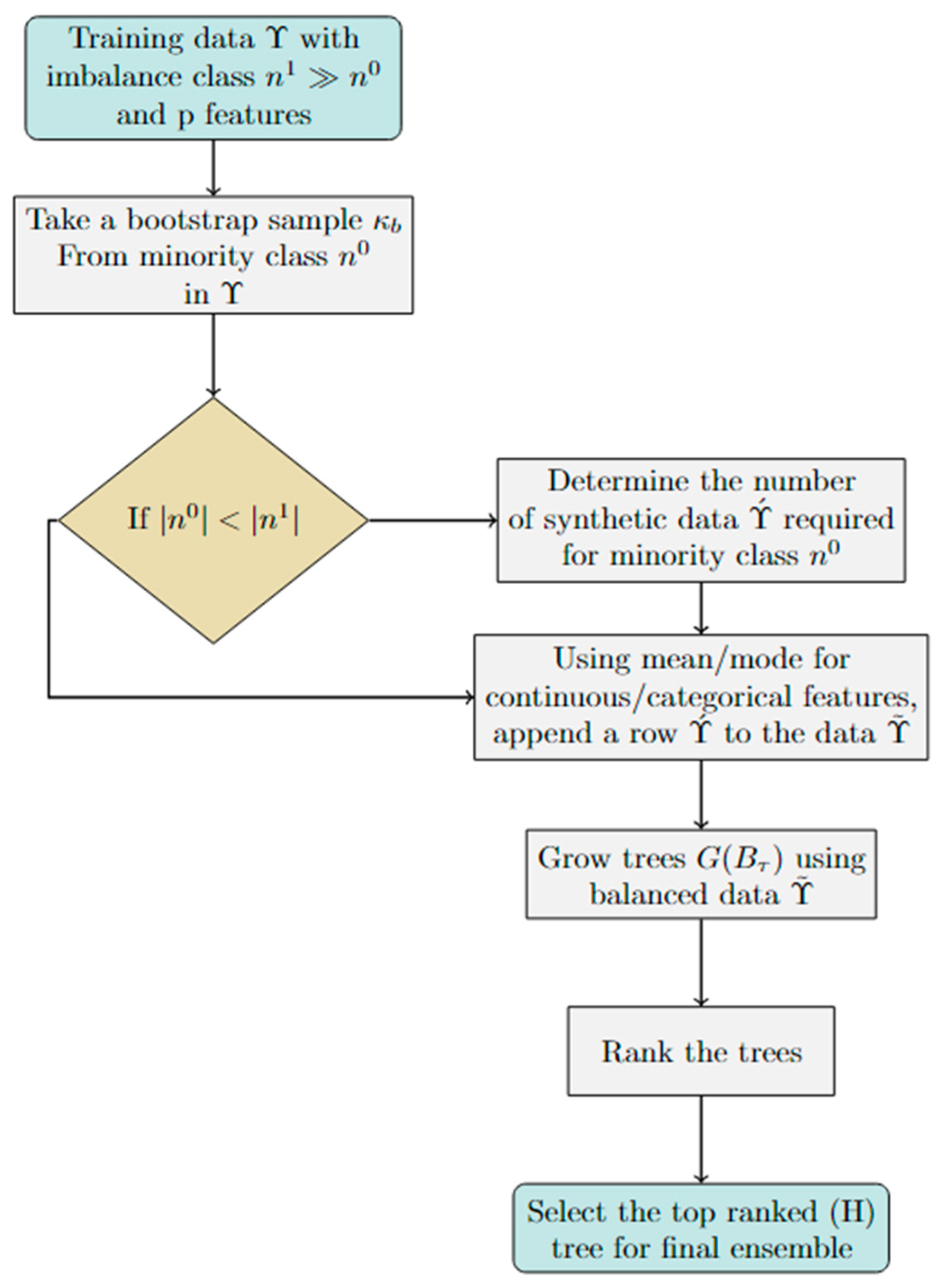
Figure 2.
Box-plots comparing and to other state-of-the-art methods, displaying the classification error rate for a range of datasets using 70% training and 30% testing.
Figure 2.
Box-plots comparing and to other state-of-the-art methods, displaying the classification error rate for a range of datasets using 70% training and 30% testing.
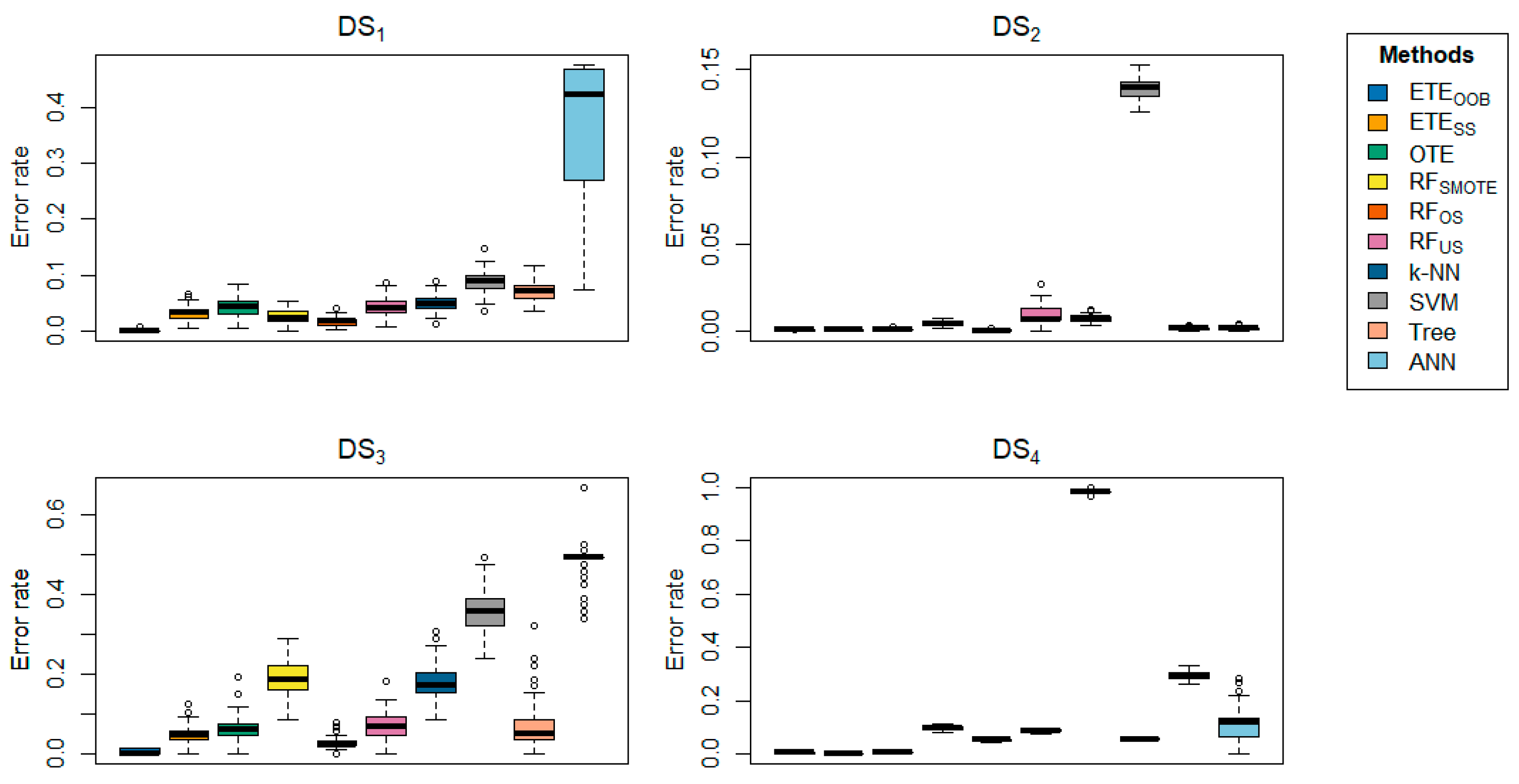
Figure 3.
Box-plots comparing and to other state-of-the-art methods, displaying the classification error rate for a range of datasets using 70% training and 30% testing.
Figure 3.
Box-plots comparing and to other state-of-the-art methods, displaying the classification error rate for a range of datasets using 70% training and 30% testing.
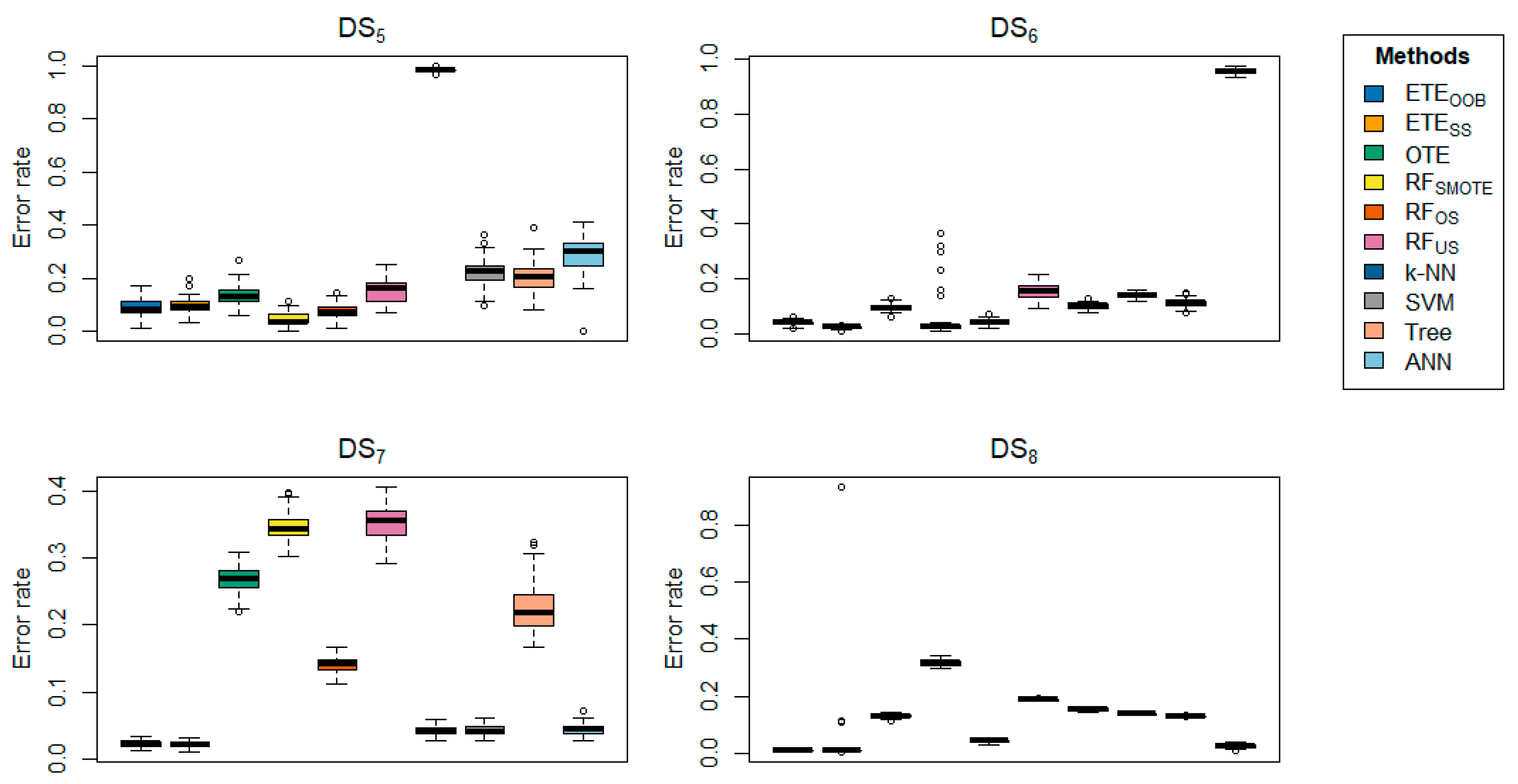
Figure 4.
Box-plots comparing and to other state-of-the-art methods, displaying the classification error rate for a range of datasets using 70% training and 30% testing.
Figure 4.
Box-plots comparing and to other state-of-the-art methods, displaying the classification error rate for a range of datasets using 70% training and 30% testing.
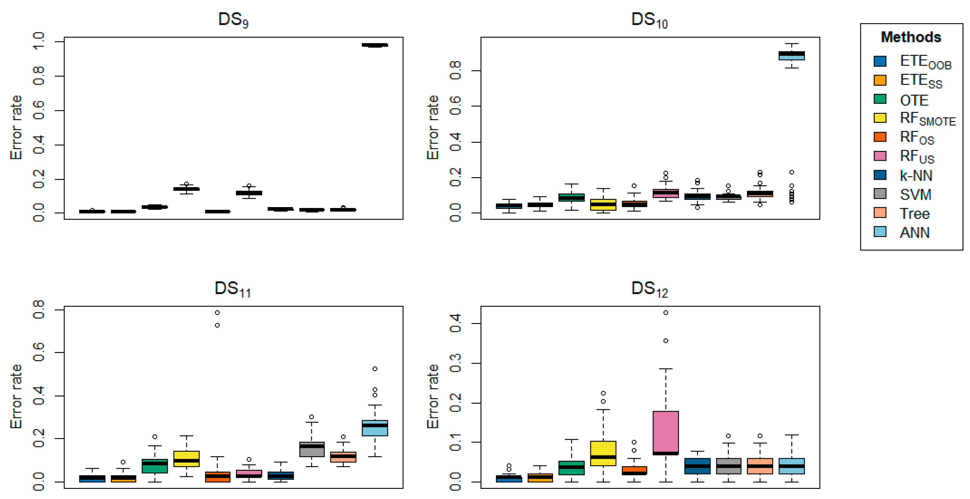
Figure 5.
Box-plots comparing and to other state-of-the-art methods, displaying the classification error rate for a range of datasets using 70% training and 30% testing.
Figure 5.
Box-plots comparing and to other state-of-the-art methods, displaying the classification error rate for a range of datasets using 70% training and 30% testing.
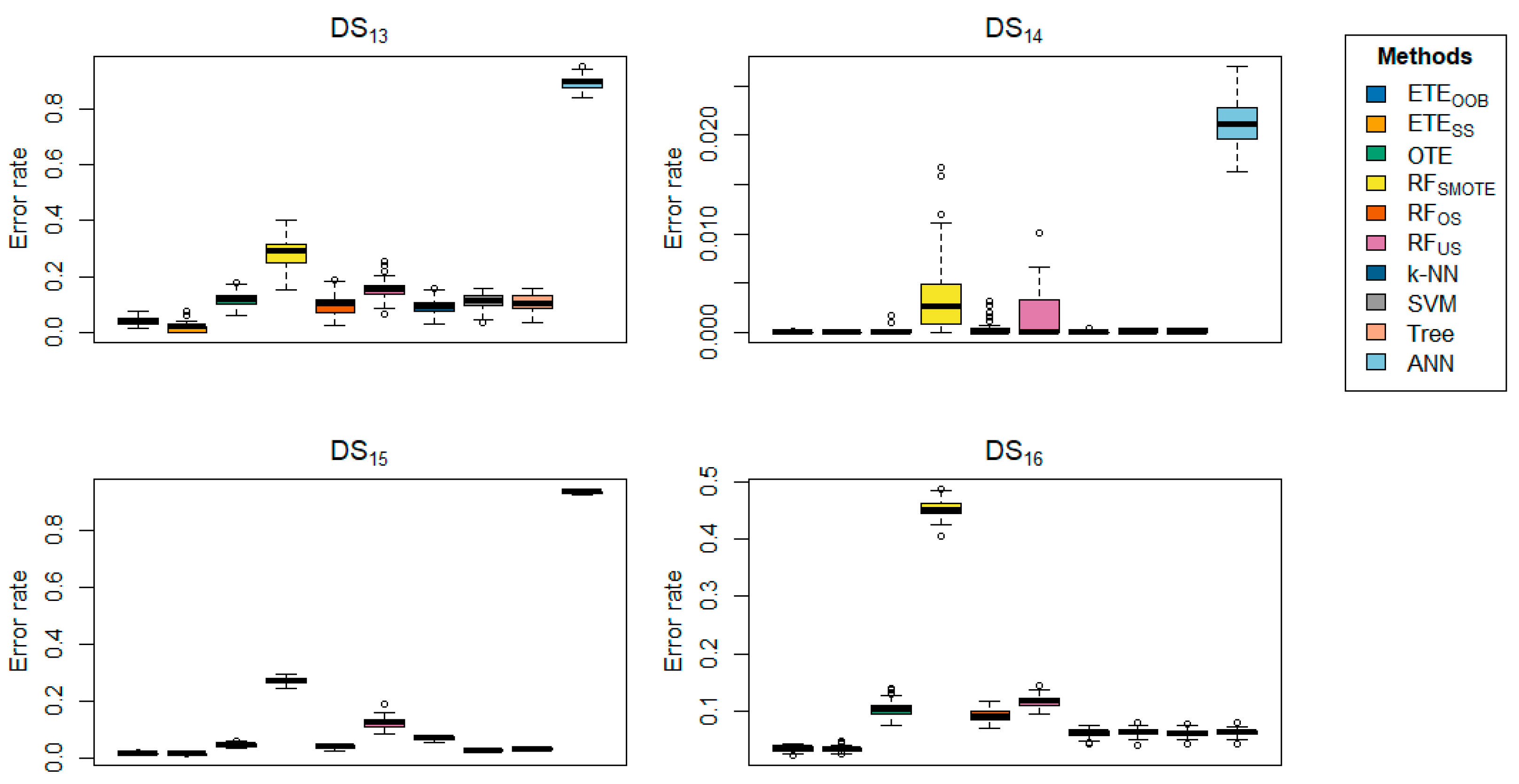
Figure 6.
Box-plots comparing and to other state-of-the-art methods, displaying the classification error rate for a range of datasets using 70% training and 30% testing.
Figure 6.
Box-plots comparing and to other state-of-the-art methods, displaying the classification error rate for a range of datasets using 70% training and 30% testing.
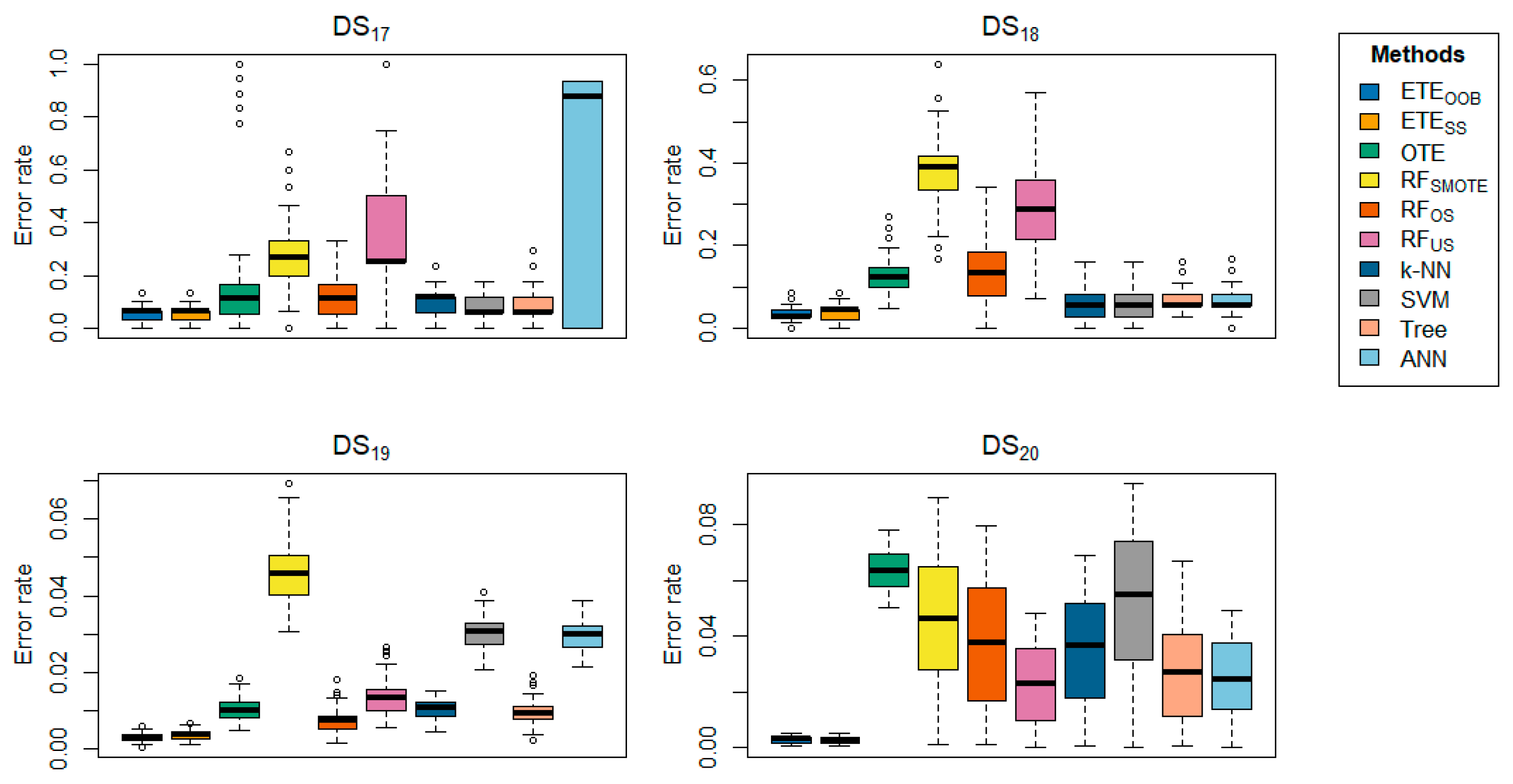
Figure 7.
Box-plots comparing and to other state-of-the-art methods, displaying the precision for a range of datasets using 70% training and 30% testing.
Figure 7.
Box-plots comparing and to other state-of-the-art methods, displaying the precision for a range of datasets using 70% training and 30% testing.
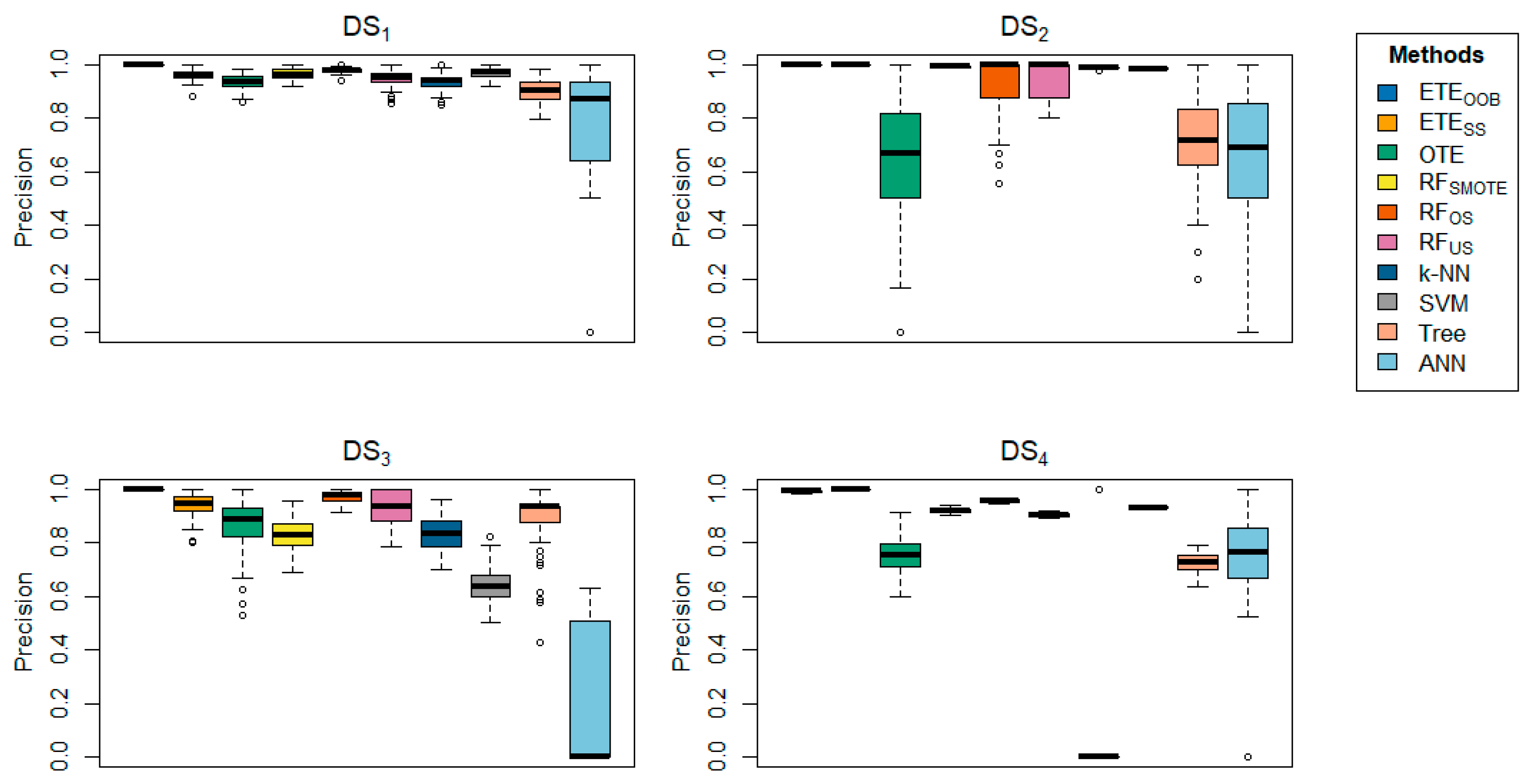
Figure 8.
Box-plots comparing and to other state-of-the-art methods, displaying the precision for a range of datasets using 70% training and 30% testing.
Figure 8.
Box-plots comparing and to other state-of-the-art methods, displaying the precision for a range of datasets using 70% training and 30% testing.

Figure 9.
Box-plots comparing and to other state-of-the-art methods, displaying the precision for a range of datasets using 70% training and 30% testing.
Figure 9.
Box-plots comparing and to other state-of-the-art methods, displaying the precision for a range of datasets using 70% training and 30% testing.
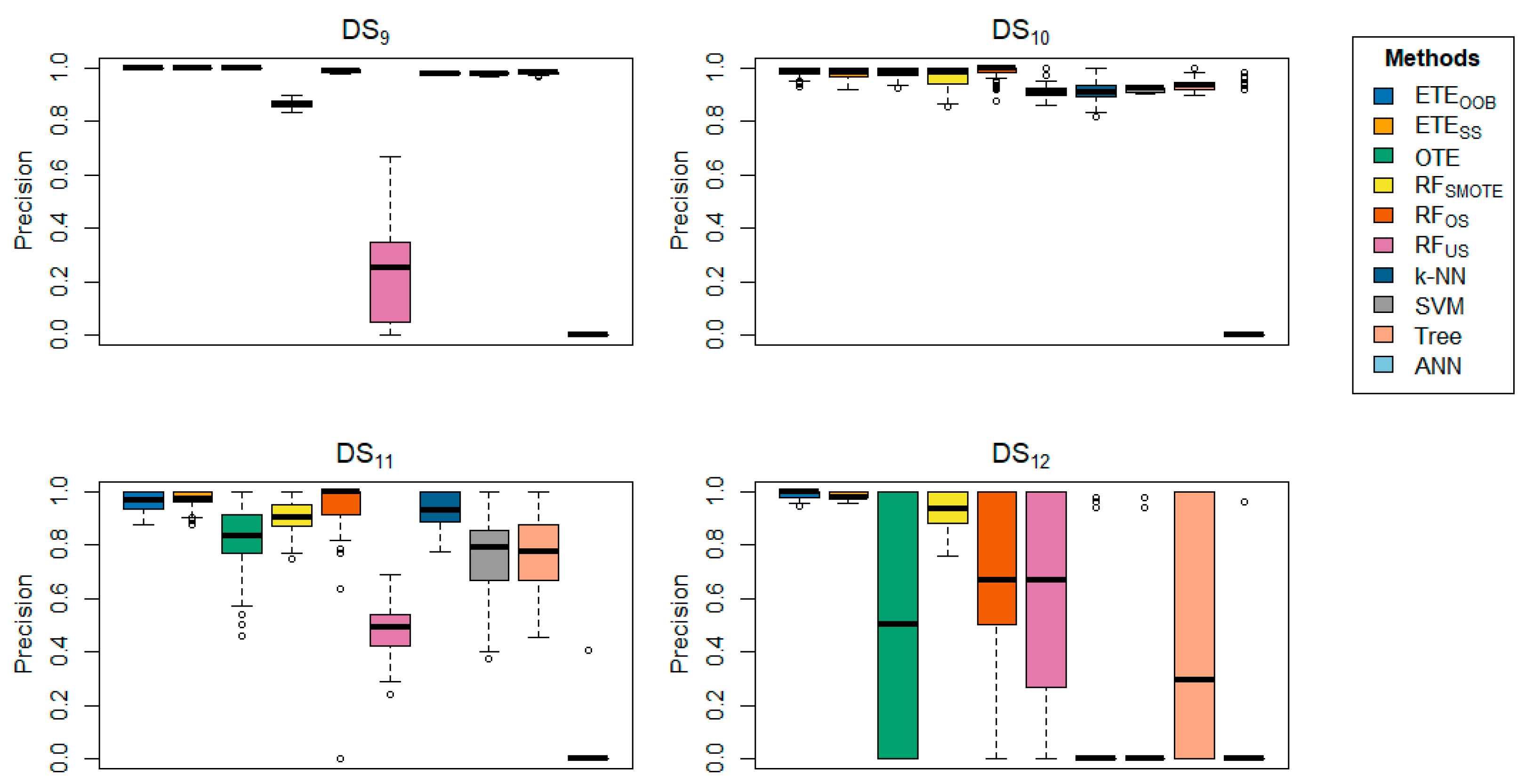
Figure 10.
Box-plots comparing and to other state-of-the-art methods, displaying the precision for a range of datasets using 70% training and 30% testing.
Figure 10.
Box-plots comparing and to other state-of-the-art methods, displaying the precision for a range of datasets using 70% training and 30% testing.

Figure 11.
Box-plots comparing and to other state-of-the-art methods, displaying the precision for a range of datasets using 70% training and 30%.
Figure 11.
Box-plots comparing and to other state-of-the-art methods, displaying the precision for a range of datasets using 70% training and 30%.
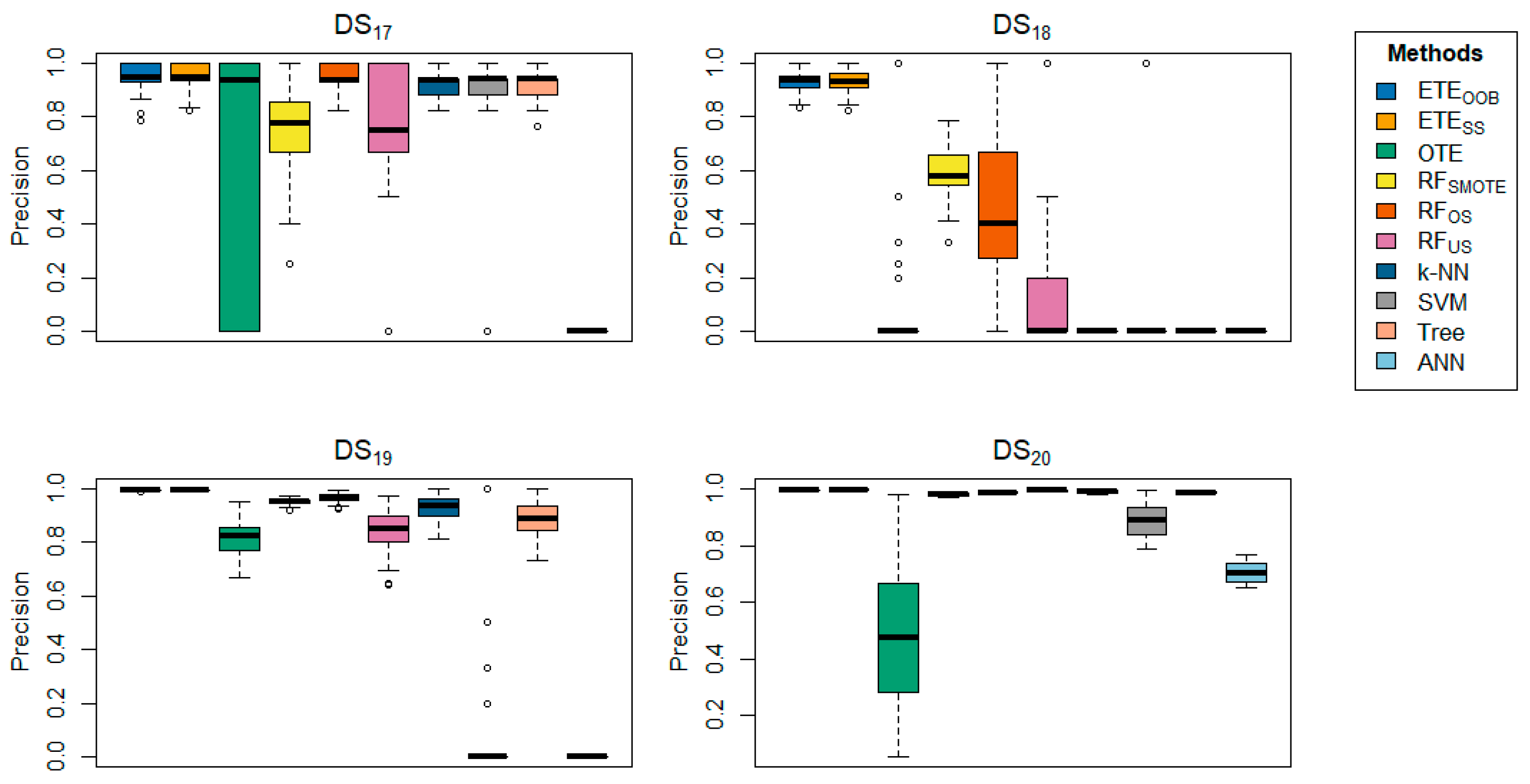
Figure 12.
A multi-line plot examines the impact of the proposed method, i.e., , varying the number of trees (H) in the ensemble on the error rate.
Figure 12.
A multi-line plot examines the impact of the proposed method, i.e., , varying the number of trees (H) in the ensemble on the error rate.
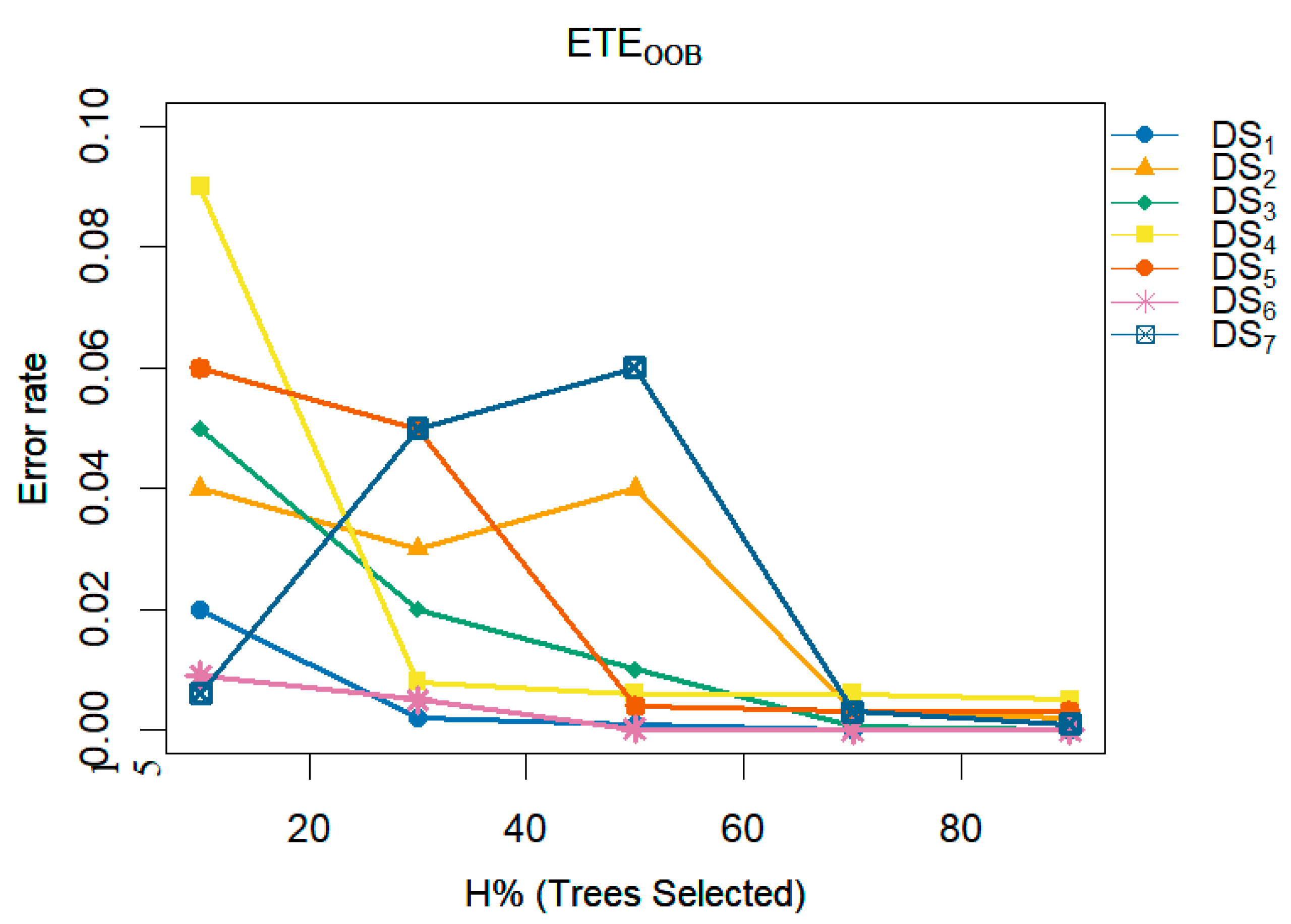
Figure 13.
A multi-line plot examines the impact of the proposed method, i.e., , varying the number of trees (H) in the ensemble on the error rate.
Figure 13.
A multi-line plot examines the impact of the proposed method, i.e., , varying the number of trees (H) in the ensemble on the error rate.
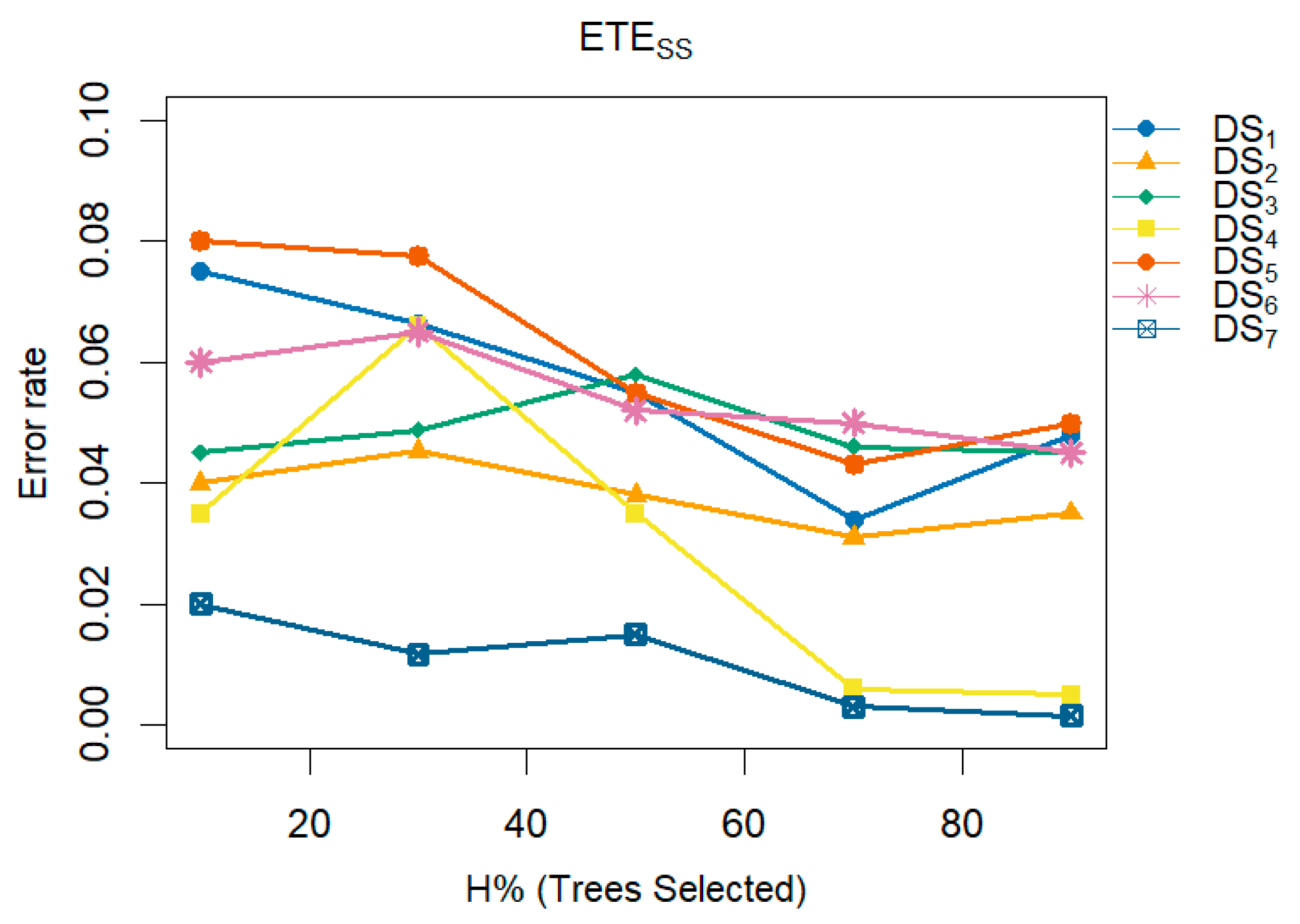
Figure 14.
Bar-plot display the proposed method, i.e., and , classification error rate and precision on both and including comparisons with other state-of-the-art techniques.
Figure 14.
Bar-plot display the proposed method, i.e., and , classification error rate and precision on both and including comparisons with other state-of-the-art techniques.
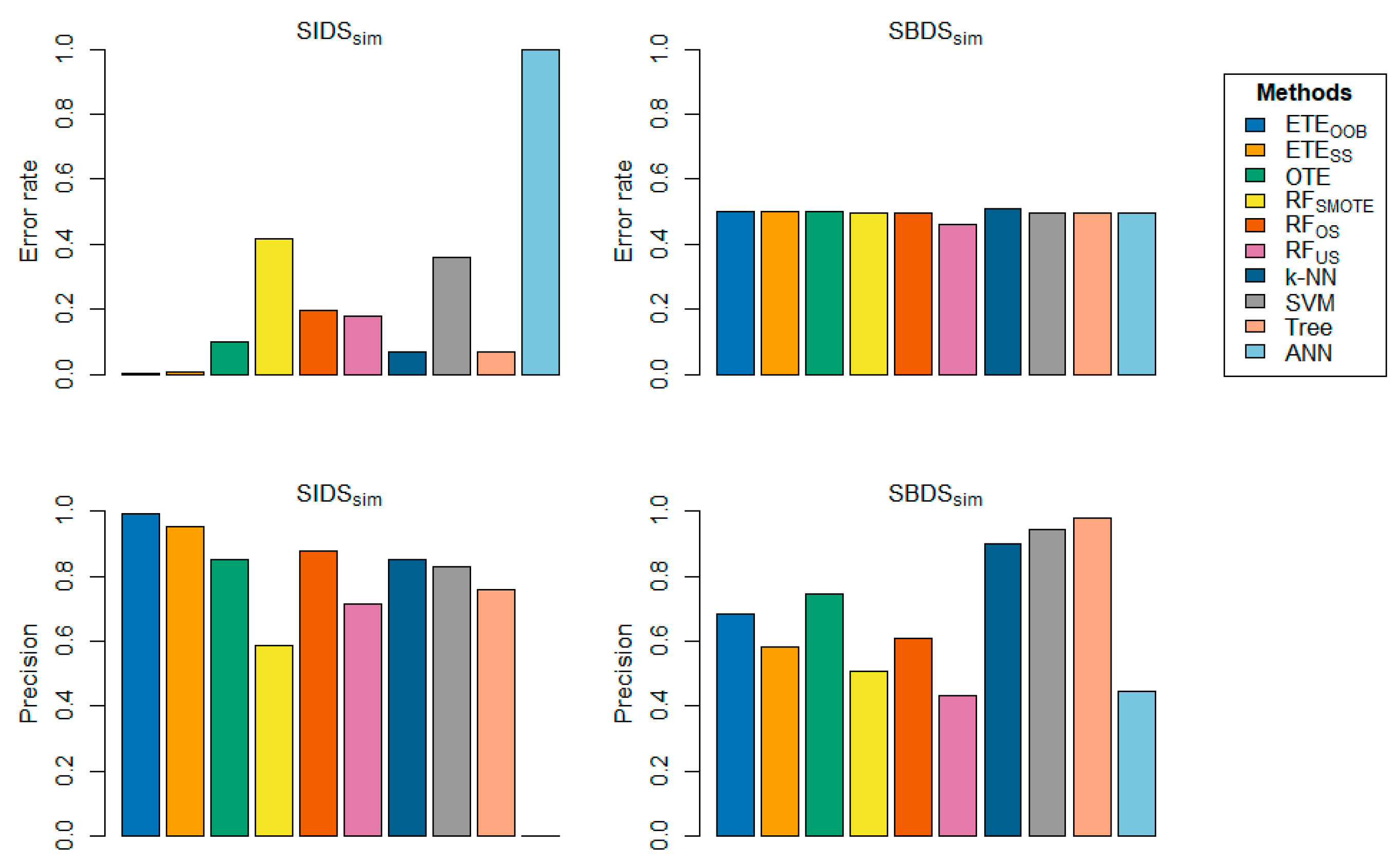

Table 1.
Summary of datasets with class-imbalanced problem.
| No | Dataset (DS) | Instances | Features | Class-based Distribution |
Source | |
|---|---|---|---|---|---|---|
| Breast Cancer | 569 | 31 | 357/212 | (1.6839:1) | https://www.kaggle.com/datasets/utkarshx27/breast-cancer-wisconsin-diagnostic-dataset | |
| Credit Card | 284807 | 30 | 284807/492 | (578.876:1) | https://www.kaggle.com/datasets/mlg-ulb/creditcardfraud | |
| Drug Classification | 200 | 6 | 145/54 | (2.685:1) | https://openml.org/search?type=data&status=active&id=43382 | |
| Eeg eye | 5856 | 14 | 5708/148 | (38.567:1) | https://openml.org/search?type=data&status=active&sort=runs&id=1471 | |
| Glass Classification | 213 | 9 | 144/69 | (2.086:1) | https://openml.org/search?type=data&status=active&id=43750 | |
| Pc4 | 1339 | 37 | 1279/60 | (21.316:1) | https://openml.org/search?type=data&status=active&sort=runs&id=1049 | |
| Madelon | 1358 | 500 | 1300/58 | (22.413:1) | https://openml.org/search?type=data&status=active&sort=runs&id=1485 | |
| Turing binary | 6384 | 20 | 6260/124 | (50.483:1) | https://www.openml.org/search?type=data&status=active&id=44269 | |
| KDD | 2566 | 35 | 2515/51 | (49.313:1) | https://openml.org/search?type=data&status=active&id=45075 | |
| Liver disorder | 220 | 6 | 200/20 | (10:1) | https://openml.org/search?type=data&status=active&id=8 | |
| Wine | 143 | 13 | 106/37 | (2.864:1) | https://archive.ics.uci.edu/dataset/109/wine | |
| Soy bean | 167 | 8 | 160/7 | (22.857:1) | https://archive.ics.uci.edu/dataset/913/forty+soybean+cultivars+from+subsequent+harvests | |
| Ionosphere | 350 | 32 | 312/38 | (8.210:1) | https://archive.ics.uci.edu/dataset/52/ionosphere | |
| Room Occupancy | 8407 | 14 | 8228/179 | (45.966:1) | https://archive.ics.uci.edu/dataset/864/room+occupancy+estimation | |
| Harth | 7269 | 7 | 6771/498 | (13.596:1) | https://archive.ics.uci.edu/dataset/779/harth | |
| Rocket League | 3015 | 6 | 2830/185 | 15.297:1 | https://archive.ics.uci.edu/dataset/858/rocket+league+skillshots | |
| Sirtuin6 | 54 | 6 | 50/4 | (12.5:1) | https://archive.ics.uci.edu/dataset/748/sirtuin6+small+molecules-1 | |
| Toxicity | 123 | 12 | 115/8 | (14.375:1) | https://archive.ics.uci.edu/dataset/728/toxicity-2 | |
| Dry bean | 4357 | 16 | 4246/129 | (32.914:1) | https://archive.ics.uci.edu/dataset/602/dry+bean+dataset | |
| Kc2 | 520 | 21 | 414/106 | (3.905:1) | https://openml.org/search?type=data&status=active&sort=runs&id=1063 |
Table 2.
Comparison of the proposed methods, and , with cutting-edge methods using 70% training and 30% testing in terms of classification error rate.
Table 2.
Comparison of the proposed methods, and , with cutting-edge methods using 70% training and 30% testing in terms of classification error rate.
| Dataset | OTE | RF(smote) | RF(over) | RF(under) | k-NN | SVM | ANN | Tree | |||||||
|---|---|---|---|---|---|---|---|---|---|---|---|---|---|---|---|
| Breast Cancer | 0.0015 | 0.0311 | 0.0427 | 0.0264 | 0.0166 | 0.0422 | 0.0851 | 0.0486 | 0.3625 | 0.0723 | |||||
| Credit Card | 0.0005 | 0.0005 | 0.0010 | 0.0046 | 0.0006 | 0.0083 | 0.1395 | 0.0071 | 0.0016 | 0.0014 | |||||
| Drug Classification | 0.0038 | 0.0461 | 0.0624 | 0.1875 | 0.0296 | 0.0650 | 0.3542 | 0.1771 | 0.4998 | 0.0697 | |||||
| Eeg eye | 0.0035 | 0 | 0.0063 | 0.0942 | 0.0521 | 0.0872 | 0.0553 | 0.9827 | 0.1094 | 0.2947 | |||||
| Glass Classification | 0.0914 | 0.0974 | 0.1330 | 0.0405 | 0.0710 | 0.1518 | 0.2194 | 0.9839 | 0.2879 | 0.1993 | |||||
| Pc4 | 0.0384 | 0.0213 | 0.0945 | 0.0411 | 0.0421 | 0.1519 | 0.1392 | 0.1006 | 0.9555 | 0.1120 | |||||
| Madelon | 0.0222 | 0.0218 | 0.2675 | 0.3459 | 0.1397 | 0.3525 | 0.0416 | 0.0420 | 0.0435 | 0.2260 | |||||
| Turing binary | 0.0102 | 0.0214 | 0.1321 | 0.3173 | 0.0437 | 0.1882 | 0.1392 | 0.1541 | 0.0271 | 0.1303 | |||||
| KDD | 0.0099 | 0.0101 | 0.0355 | 0.1394 | 0.0098 | 0.1191 | 0.0198 | 0.0226 | 0.9804 | 0.0185 | |||||
| Liver disorder | 0.0400 | 0.0453 | 0.0864 | 0.0469 | 0.0512 | 0.1153 | 0.0862 | 0.0915 | 0.7661 | 0.1126 | |||||
| Wine | 0.0227 | 0.0173 | 0.0796 | 0.1029 | 0.0680 | 0.0324 | 0.1605 | 0.0305 | 0.2574 | 0.1235 | |||||
| Soy bean | 0.0093 | 0.0100 | 0.0364 | 0.0706 | 0.0308 | 0.1229 | 0.0416 | 0.0420 | 0.0428 | 0.0402 | |||||
| Ionosphere | 0.0429 | 0.0172 | 0.1168 | 0.2830 | 0.0985 | 0.1531 | 0.1107 | 0.0898 | 0.8913 | 0.1093 | |||||
| Room Occupancy | 0 | 0 | 0.0002 | 0.0034 | 0.0003 | 0.0020 | 0.0001 | 0.00001 | 0.0211 | 0.0002 | |||||
| Harth | 0.0121 | 0.0119 | 0.0438 | 0.2698 | 0.0379 | 0.1214 | 0.0253 | 0.0682 | 0.9318 | 0.0303 | |||||
| Rocket League | 0.0334 | 0.0331 | 0.1032 | 0.4525 | 0.0914 | 0.1158 | 0.0622 | 0.0616 | 0.0614 | 0.0613 | |||||
| Sirtuin6 | 0.0516 | 0.0516 | 0.2433 | 0.2680 | 0.1200 | 0.3275 | 0.0700 | 0.0965 | 0.6519 | 0.0847 | |||||
| Toxicity | 0.0339 | 0.0352 | 0.1241 | 0.3828 | 0.1392 | 0.2750 | 0.0645 | 0.0570 | 0.0694 | 0.0692 | |||||
| Dry bean | 0.0030 | 0.0035 | 0.0102 | 0.0500 | 0.0075 | 0.0134 | 0.0301 | 0.0103 | 0.0295 | 0.0091 | |||||
| Kc2 | 0.0029 | 0.0026 | 0.0639 | 0.0459 | 0.0384 | 0.0236 | 0.0519 | 0.0353 | 0.0250 | 0.0277 | |||||
Table 3.
Comparison of the proposed methods, and , with cutting-edge methods using 70% training and 30% testing in terms of precision.
Table 3.
Comparison of the proposed methods, and , with cutting-edge methods using 70% training and 30% testing in terms of precision.
| Dataset | OTE | RF(smote) | RF(over) | RF(under) | k-NN | SVM | ANN | Tree | ||||
|---|---|---|---|---|---|---|---|---|---|---|---|---|
| Breast Cancer | 1.0000 | 0.9629 | 0.9364 | 0.9670 | 0.9795 | 0.9517 | 0.9696 | 0.9353 | 0.7200 | 0.9029 | ||
| Credit Card | 0.9993 | 0.9992 | 0.6503 | 0.9923 | 0.9241 | 0.9505 | 0.9860 | 0.9889 | 0.6123 | 0.7284 | ||
| Drug Classification | 1.0000 | 0.9378 | 0.8655 | 0.8277 | 0.9714 | 0.9361 | 0.6401 | 0.8328 | 0.2006 | 0.9031 | ||
| Eeg eye | 0.9929 | 1 | 0.7578 | 0.9216 | 0.9576 | 0.9049 | 0.9327 | 0.0700 | 0.6646 | 0.7257 | ||
| Glass Classification | 0.9153 | 0.9022 | 0.8050 | 0.9739 | 0.8984 | 0.8166 | 0.6440 | 0.1300 | 0.2665 | 0.7204 | ||
| Pc4 | 0.9981 | 0.9971 | 0.9755 | 0.9904 | 0.9885 | 0.9059 | 0.8811 | 0.9207 | 0 | 0.9287 | ||
| Madelon | 0.9554 | 0.9563 | 0.4063 | 0.6586 | 0.8614 | 0.6449 | 0.1750 | 0.0192 | 0 | 0.7171 | ||
| Turing binary | 0.9796 | 0.9799 | 0.0162 | 0.6648 | 0.9757 | 0.4800 | 0.2519 | 0.2176 | 0.0541 | 0.0140 | ||
| KDD | 1 | 1 | 0.9987 | 0.8649 | 0.9896 | 0.2506 | 0.9802 | 0.9794 | 0 | 0.9830 | ||
| Liver disorder | 0.9860 | 0.9830 | 0.9835 | 0.9713 | 0.9835 | 0.9134 | 0.9206 | 0.9135 | 0.1604 | 0.9365 | ||
| Wine | 0.9584 | 0.9720 | 0.8302 | 0.9111 | 0.9187 | 0.9218 | 0.7678 | 0.9296 | 0.0041 | 0.7702 | ||
| Soy bean | 0.9888 | 0.9864 | 0.4845 | 0.9309 | 0.6332 | 0.5975 | 0.0286 | 0.0288 | 0.0096 | 0.3968 | ||
| Ionosphere | 0.9733 | 0.6763 | 0.9292 | 0.7239 | 0.9589 | 0.9209 | 0.8954 | 0.9137 | 0 | 0.9397 | ||
| Room Occupancy | 1 | 1 | 0.9971 | 0.9962 | 0.9971 | 0.9936 | 0.9943 | 1 | 0 | 0.9948 | ||
| Harth | 0.9980 | 0.9976 | 0.9750 | 0.7336 | 0.9828 | 0.9190 | 0.9800 | 0.9317 | 0 | 0.9749 | ||
| Rocket League | 0.9336 | 0.9362 | 0.0759 | 0.5431 | 0.3916 | 0.0890 | 0.1240 | 0 | 0 | 0 | ||
| Sirtuin6 | 0.9554 | 0.9589 | 0.6373 | 0.7638 | 0.9509 | 0.7683 | 0.9200 | 0.9235 | 0 | 0.9182 | ||
| Toxicity | 0.9323 | 0.9314 | 0.0386 | 0.5924 | 0.4527 | 0.1049 | 0.0100 | 0 | 0 | 0 | ||
| Dry bean | 0.9961 | 0.9952 | 0.8161 | 0.9503 | 0.9639 | 0.9702 | 0.0353 | 0.9283 | 0 | 0.8880 | ||
| Kc2 | 0.9948 | 0.9952 | 0.4885 | 0.9793 | 0.9853 | 0.9925 | 0.8869 | 0.9895 | 0.7053 | 0.9869 | ||
Table 4.
Comparison of the proposed methods, and , with cutting-edge methods using 90% training and 10% testing in terms of classification error rate.
Table 4.
Comparison of the proposed methods, and , with cutting-edge methods using 90% training and 10% testing in terms of classification error rate.
| Dataset | OTE | RF(smote) | RF(over) | RF(under) | k-NN | SVM | ANN | Tree | ||
|---|---|---|---|---|---|---|---|---|---|---|
| Breast Cancer | 0.0261 | 0.0108 | 0.1827 | 0.0229 | 0.0069 | 0.0072 | 0.0259 | 0.0358 | 0.5105 | 0.0241 |
| Credit Card | 0.0312 | 0.0028 | 0.1343 | 0.0177 | 0.0134 | 0.006 | 0.0224 | 0.033 | 0.4165 | 0.026 |
| Drug Classification | 0.0041 | 0.0003 | 0.0042 | 0.0459 | 0.0267 | 0.0046 | 0.0046 | 0.0042 | 0.042 | 0.0026 |
| Eeg eye | 0.0176 | 0.010 | 0.039 | 0.0494 | 0.0207 | 0.0191 | 0.0379 | 0.0374 | 0.2532 | 0.1108 |
| Glass Classification | 0.0048 | 0.0059 | 0.0188 | 0.0245 | 0.047 | 0.0407 | 0.0749 | 0.3964 | 0.0996 | 0.1457 |
| Pc4 | 0.0009 | 0.0038 | 0.0382 | 0.0327 | 0.0349 | 0.0261 | 0.0373 | 0.0063 | 0.0231 | 0.0256 |
| Madelon | 0.0043 | 0.0001 | 0.0077 | 0.016 | 0.0048 | 0.0318 | 0.0062 | 0.0479 | 0.0406 | 0.0186 |
| Turing binary | 0.0018 | 0.0001 | 0.0225 | 0.0004 | 0.0034 | 0.0064 | 0.0163 | 0.0295 | 0.0182 | 0.0434 |
| KDD | 0.0019 | 0.0009 | 0.0336 | 0.0001 | 0.003 | 0.0128 | 0.0122 | 0.0456 | 0.015 | 0.0464 |
| Liver disorder | 0.0002 | 0.005 | 0.0072 | 0.0008 | 0.0009 | 0.0366 | 0.0231 | 0.0221 | 0.0406 | 0.0282 |
| Wine | 0.0026 | 0.0356 | 0.0217 | 0.0087 | 0.0384 | 0.0091 | 0.0405 | 0.0241 | 0.0146 | 0.0306 |
| Soy bean | 0.0005 | 0.0413 | 0.0137 | 0.033 | 0.0152 | 0.0141 | 0.0454 | 0.2376 | 0.1533 | 0.4282 |
| Ionosphere | 0.0007 | 0.0014 | 0.0017 | 0.0035 | 0.0006 | 0.0004 | 0.0015 | 0.0015 | 0.0008 | 0.001 |
| Room Occupancy | 0.0001 | 0.0046 | 0.0029 | 0.0028 | 0.004 | 0.0002 | 0.0013 | 0.0045 | 0.0048 | 0.0432 |
| Harth | 0.0003 | 0.011 | 0.0231 | 0.0011 | 0.0337 | 0.002 | 0.0294 | 0.0064 | 0.0285 | 0.0094 |
| Rocket League | 0.0032 | 0.0068 | 0.0334 | 0.0104 | 0.0499 | 0.0233 | 0.0169 | 0.0115 | 0.0513 | 0.0423 |
| Sirtuin6 | 0.0021 | 0.0325 | 0.0291 | 0.0162 | 0.0029 | 0.0325 | 0.0172 | 0.0069 | 0.1549 | 0.0219 |
| Toxicity | 0.0219 | 0.0259 | 0.0143 | 0.1353 | 0.0312 | 0.3115 | 0.1628 | 0.0619 | 0.4473 | 0.4854 |
| Dry bean | 0.0005 | 0.0683 | 0.1644 | 0.0418 | 0.3127 | 0.0238 | 0.1366 | 0.437 | 0.2924 | 0.2128 |
| Kc2 | 0.0001 | 0.0499 | 0.042 | 0.0021 | 0.0144 | 0.012 | 0.0076 | 0.0438 | 0.0066 | 0.0265 |
Table 5.
Comparison of the proposed methods, and , with cutting-edge methods using 90% training and 10% testing in terms of precision.
Table 5.
Comparison of the proposed methods, and , with cutting-edge methods using 90% training and 10% testing in terms of precision.
| Dataset | OTE | RF(smote) | RF(over) | RF(under) | k-NN | SVM | ANN | Tree | ||
|---|---|---|---|---|---|---|---|---|---|---|
| Breast Cancer | 0.9947 | 0.9947 | 0.6517 | 0.839 | 0.8804 | 0.838 | 0.8338 | 0.913 | 0.2983 | 0.8999 |
| Credit Card | 0.9896 | 0.9956 | 0.6501 | 0.8423 | 0.8884 | 0.8429 | 0.8354 | 0.9143 | 0.3128 | 0.9013 |
| Drug Classification | 0.9859 | 0.9898 | 0.7349 | 0.8767 | 0.9354 | 0.8716 | 0.8433 | 0.9266 | 0.4999 | 0.9079 |
| Eeg eye | 0.9785 | 0.9896 | 0.7333 | 0.8822 | 0.9386 | 0.8639 | 0.8457 | 0.9136 | 0.5117 | 0.9074 |
| Glass Classification | 0.9999 | 1 | 0.9998 | 0.8915 | 0.9406 | 0.9334 | 0.9542 | 0.97 | 0.7993 | 0.6966 |
| Pc4 | 0.9036 | 0.9139 | 0.8982 | 0.9492 | 0.9718 | 0.8841 | 0.8656 | 0.98 | 0.7396 | 0.8371 |
| Madelon | 1 | 0.9604 | 0.4013 | 0.9645 | 0.9104 | 0.7624 | 0.2103 | 0.6461 | 0.0445 | 0.5508 |
| Turing binary | 1 | 1 | 0.9197 | 0.6508 | 0.8596 | 0.6509 | 0.9591 | 0.6373 | 0.9565 | 0.8013 |
| KDD | 1 | 0.9999 | 0.9962 | 0.7037 | 0.949 | 0.8174 | 0.8721 | 0.8737 | 0.9815 | 0.8699 |
| Liver disorder | 0.9803 | 0.9798 | 0.2393 | 0.8568 | 0.9942 | 0.9056 | 0.1289 | 0.1582 | 0.0196 | 0.6431 |
| Wine | 0.9338 | 0.9264 | 0.2349 | 0.9372 | 0.8929 | 0.6402 | 0.3683 | 0.2322 | 0.1582 | 0.3683 |
| Soy bean | 1 | 0.994 | 0.9536 | 0.8912 | 0.9757 | 0.9665 | 0.8608 | 0.9704 | 0.7479 | 0.9216 |
| Ionosphere | 0.9922 | 0.9937 | 0.8841 | 0.0706 | 0.9889 | 0.9364 | 0.9586 | 0.958 | 0.9572 | 0.9765 |
| Room Occupancy | 0.9413 | 0.9988 | 0.5066 | 0.283 | 0.6602 | 0.5903 | 0.2519 | 0.8307 | 0.1087 | 0.5031 |
| Harth | 0.9999 | 1 | 0.9999 | 0.0034 | 0.9998 | 0.9992 | 1 | 0.9999 | 0.9788 | 0.9999 |
| Rocket League | 0.9775 | 0.9786 | 0.6987 | 0.2698 | 0.8552 | 0.7579 | 0.8854 | 0 | 0.0681 | 0.8709 |
| Sirtuin6 | 0.9995 | 0.9976 | 0.9505 | 0.4525 | 0.958 | 0.9407 | 0.9396 | 0.9383 | 0.9385 | 0.9386 |
| Toxicity | 0.9428 | 0.9394 | 0.09 | 0.268 | 0.6491 | 0.2142 | 0 | 0 | 0.3481 | 0 |
| Dry bean | 0.9994 | 0.9986 | 0.9074 | 0.3828 | 0.9502 | 0.8546 | 0.9369 | 0.9429 | 0.9305 | 0.9313 |
| Kc2 | 0.9999 | 1 | 0.9911 | 0.8849 | 0.9251 | 0.9725 | 0.942 | 0.004 | 0.6507 | 0.5571 |
Disclaimer/Publisher’s Note: The statements, opinions and data contained in all publications are solely those of the individual author(s) and contributor(s) and not of MDPI and/or the editor(s). MDPI and/or the editor(s) disclaim responsibility for any injury to people or property resulting from any ideas, methods, instructions or products referred to in the content. |
© 2024 by the authors. Licensee MDPI, Basel, Switzerland. This article is an open access article distributed under the terms and conditions of the Creative Commons Attribution (CC BY) license (http://creativecommons.org/licenses/by/4.0/).
Copyright: This open access article is published under a Creative Commons CC BY 4.0 license, which permit the free download, distribution, and reuse, provided that the author and preprint are cited in any reuse.


