1. Introduction
In the dynamic realm of customer-centric industries, predicting and mitigating customer churn has become a critical challenge. Customer churn, defined as the discontinuation of a customer's association with a product or service, significantly affects a company's revenue and growth potential. Given the higher costs associated with acquiring new customers compared to retaining existing ones, businesses increasingly rely on machine learning (ML) models to develop robust churn prediction systems. These models enable the identification of at-risk customers, facilitating targeted interventions to improve retention and loyalty.
This challenge spans multiple industries, including banking, insurance, and telecommunications. Within the telecommunications sector, a cornerstone of global socioeconomic development and a significant contributor to revenue generation, the financial scale reaches approximately
$4.7 trillion annually [
1,
2]. The sector faces intense competition as companies strive to grow their market share by expanding customer bases. Customer retention has become a primary goal of customer relationship management (CRM) initiatives, as retaining customers is up to 20 times more cost-effective than acquiring new ones [
1]. Consequently, minimizing customer churn is essential for optimizing revenue and reducing marketing and advertising expenditures.
The application of ML models in churn prediction has garnered substantial attention, addressing the binary classification task of identifying churn and non-churn customers. Popular models include Decision Trees [
3,
4,
5,
6,
7,
8,
9,
10,
11], Artificial Neural Networks [
3,
4,
10,
11,
12], Random Forests [
13,
14], Support Vector Machines [
11], and advanced boosting techniques such as eXtreme Gradient Boosting (XGBoost) [
15], Light Gradient Boosting Machine (LightGBM) [
16], and Categorical Boosting (CatBoost) [
17]. Each model exhibits distinct strengths and limitations, influenced by factors such as dataset characteristics, customer behavior complexity, and specific prediction objectives [
18,
19].
A major challenge in churn prediction arises from class imbalance, where churned customers are vastly outnumbered by non-churned customers. This imbalance skews model performance and affects predictive accuracy. To address this, various resampling techniques have been applied, including Synthetic Minority Over-sampling Technique (SMOTE) [
20], Adaptive Synthetic Sampling (ADASYN) [
21], Gaussian Noise Upsampling (GNUS) [
22], and hybrid methods such as SMOTE combined with Tomek Links [
23] or Edited Nearest Neighbors (ENN) [
24]. These techniques aim to balance datasets and improve model efficacy [
25,
26]. Furthermore, hyperparameter optimization techniques such as Grid Search, Random Search, and more advanced methods like Bayesian Optimization, Genetic Algorithms, and Hyperparameter optimization are critical for enhancing model performance [
27,
28].
Ensemble methods, particularly boosting and bagging algorithms, have proven highly effective in tackling classification problems [
29,
30,
31,
32,
33]. While numerous studies have reviewed machine learning techniques for imbalanced datasets [
25,
34,
35,
36,
37,
38,
39,
40], none have examined their performance across datasets with varying levels of imbalance, ranging from moderate to extreme. This study fills that gap by evaluating the performance of supervised classifiers, specifically Random Forest and XGBoost, combined with over-sampling techniques such as SMOTE, ADASYN, and GNUS. The analysis spans datasets with churn rates ranging from 15% to 1%. To further improve predictive accuracy, Grid Search is employed for hyperparameter optimization in these imbalanced scenarios.
This research provides a significant contribution to the field of customer churn prediction by undertaking a comprehensive evaluation of various supervised ML classifiers, specifically Random Forests and XGBoost. The study is uniquely focused on integrating these classifiers with advanced oversampling techniques such as SMOTE, ADASYN, and GNUS, while simultaneously leveraging Grid Search for hyperparameter optimization. This multifaceted analytical approach is designed to improve churn prediction accuracy, particularly in scenarios where datasets exhibit high levels of class imbalance—a common and critical challenge in real-world applications.
The research fills an important gap in the existing literature, which, while extensive in its exploration of customer churn prediction, lacks a detailed analysis of how specific ML classifiers like XGBoost and Random Forest perform under varying degrees of dataset imbalance. Although sampling methods such as SMOTE, ADASYN, and GNUS are widely employed, there remains limited understanding of their interaction with these classifiers, particularly across datasets with different imbalance ratios. Furthermore, most prior studies have not adequately addressed the influence of dataset imbalance on predictive accuracy, nor have they thoroughly examined the robustness of these classifiers when combined with advanced sampling techniques and optimized hyperparameters.
By systematically investigating these aspects, this study aims to bridge the knowledge gap and offer actionable insights into the performance dynamics of these models. The research evaluates the behavior of XGBoost and Random Forest in conjunction with sampling methods across a spectrum of imbalance scenarios, ranging from moderate to extreme. This detailed examination not only underscores the importance of dataset characteristics in determining model efficacy but also highlights the critical role of oversampling techniques and hyperparameter tuning in achieving accurate and reliable predictions.
This study focuses on Random Forest and XGBoost due to their well-established performance in customer churn prediction and imbalanced classification. The rationale for selecting these two models is based on the following considerations:
Established Benchmark Models: Random Forest and XGBoost have been extensively utilized in customer churn prediction and imbalanced classification tasks due to their interpretability, robustness, and efficiency. Numerous prior studies, including our recent work [
39], have demonstrated their effectiveness in handling structured tabular data, making them strong benchmark models for this study. Our previous study [
39], conducted on the same dataset, revealed that Random Forest outperforms several traditional machine learning models, including Artificial Neural Networks, Decision Trees, Support Vector Machines, and Logistic Regression. Additionally, XGBoost demonstrated superior performance compared to other boosting-based models, such as LightGBM and CatBoost. These findings reinforce the suitability of Random Forest and XGBoost as the primary models for this research.
Computational Efficiency: While deep learning models such as Convolutional Neural Networks (CNNs) and Recurrent Neural Networks (RNNs) have shown promise in various predictive tasks, they typically require significantly larger datasets, greater computational resources, and extensive hyperparameter tuning to achieve optimal performance. Given the structured nature of the customer churn dataset and its relatively limited size, tree-based ensemble methods such as Random Forest and XGBoost offer a more efficient and practical alternative. Their ability to handle imbalanced datasets with effective sampling techniques makes them particularly well-suited for this study.
By selecting Random Forest and XGBoost, this research ensures a focused and comprehensive evaluation of widely recognized and computationally efficient models in the context of customer churn prediction under varying levels of class imbalance.
The contributions of this paper are twofold. First, it provides a nuanced understanding of the interaction between ML classifiers, oversampling techniques, and dataset imbalance, which has implications for designing more effective churn prediction models. Second, it delivers a practical framework for practitioners in the telecommunications industry, enabling them to develop predictive systems that are better equipped to handle the challenges posed by highly imbalanced datasets. By doing so, this research supports the broader goal of improving customer retention strategies, reducing churn rates, and fostering sustainable growth within subscription-based businesses.
While this study focuses on customer churn prediction in the telecommunications industry, class imbalance is a widespread issue across multiple domains. In healthcare, rare disease detection often suffers from extreme class imbalance, making it difficult for models to identify positive cases. Similarly, in fraud detection, fraudulent transactions constitute a small fraction of overall transactions, requiring effective oversampling techniques to enhance detection accuracy. In finance, predicting credit defaults also involves imbalanced datasets, where misclassification of minority cases can lead to financial risk. Addressing class imbalance in these fields is critical, and while our study evaluates and compares multiple resampling techniques, including SMOTE, ADASYN, and the proposed GNUS within a telecommunications context, the insights gained from these methods have the potential to be applied across various domains facing similar data challenges.
The structure of this paper is organized as follows:
Section 2 provides an overview of ensemble machine learning techniques, imbalanced data challenges, sampling techniques, hyperparameter optimization, and evaluation metrics.
Section 3 describes the dataset and outlines the data preprocessing steps.
Section 4 presents a detailed discussion of the methodological framework, including data splitting, feature selection, and the creation of highly imbalanced datasets using random undersampling and KMeans clustering approaches.
Section 5 analyzes the experimental results, evaluating the performance of different models across four datasets with varying levels of imbalance. This section also includes statistical tests, such as the Friedman and Nemenyi tests, followed by an overall comparison, performance analysis, and summary of findings.
Section 6 outlines the conclusions of the study, while
Section 7 discusses current challenges and potential directions for future research.
2. Background
2.1. Ensemble Machine Learning Techniques
Ensemble learning, a cornerstone technique within the ML landscape, operates on the principle of synthesizing the predictions from multiple learning algorithms to form a more potent, composite model. This methodology leverages the collective strengths of various base learners, often simple or weak models, to construct an ensemble that surpasses the performance of any single model in isolation [
41]. The foundational premise of ensemble learning is rooted in the notion that a diverse array of models, when judiciously combined, can compensate for individual weaknesses, leading to superior overall predictive capabilities [
42,
43].
Contemporary research has firmly established ensemble learning as a quintessential approach for elevating the precision of predictive models in ML. Among its methodologies, bagging (Bootstrap Aggregating) such as Random Forest and boosting such as XGBoost stand out as two principal strategies, each designed to bolster model accuracy through distinct mechanisms [
29,
30]. Bagging aims to enhance model stability and accuracy by generating multiple subsets of data from the original dataset through bootstrapping. These subsets are then used to train multiple models, whose predictions are aggregated to produce a final decision, typically through majority voting for classification or averaging for regression tasks [
44].
Boosting, on the other hand, sequentially trains models, where each subsequent model attempts to correct the errors of its predecessor. This technique incrementally builds a strong classifier from a series of weak ones, by focusing more heavily on instances that were previously misclassified, thus improving the model's accuracy on challenging cases [
45]. Notable examples of boosting algorithms include AdaBoost (Adaptive Boosting) and Gradient Boosting machines, such as XGBoost which have been widely acknowledged for their effectiveness in various predictive tasks across different domains [
46,
47,
48].
The efficacy of ensemble methods extends beyond mere accuracy improvements. These techniques have also been shown to significantly reduce overfitting, a common pitfall in ML models, by introducing model diversity and focusing on robust generalization [
49]. Furthermore, ensemble learning is adaptable to both classification and regression problems, making it a versatile tool in the ML toolkit.
The strategic application of ensemble methods, particularly bagging and boosting, has led to notable advancements in predictive modelling, with numerous studies corroborating their effectiveness across a range of applications from bioinformatics to financial forecasting [
50,
51]. As ML continues to evolve, the exploration of novel ensemble techniques and their integration with emerging models and algorithms remains a vibrant area of research, promising further enhancements in predictive performance and model robustness.
2.1.1. Random Forest
The framework of Random Forest, initially conceptualized by Ho in 1995 [
13], has undergone continual refinement and development, significantly propelled by Leo Breiman's contributions in 2001 [
14]. As a sophisticated ensemble learning methodology, Random Forest leverages an extensive collection of Decision Trees for performing classification tasks, with its predictive outcome derived from the consensus across the multitude of trees. Typically, Random Forests are recognized for their enhanced performance metrics in comparison to singular Decision Tree models, although the efficacy of these forests can be markedly influenced by the specific attributes of the dataset in question.
Incorporating the bagging (Bootstrap Aggregating) strategy within its algorithmic structure, Random Forests execute by generating multiple subsets from the original training set, , through bootstrap sampling. This process is iterated B times, each cycle selecting a bootstrap sample from and employing these samples to train distinct Decision Trees:
From the training set, n examples, denoted as , are sampled with replacement.
A classification tree, pertinent to churn prediction scenarios, fb, is trained utilizing the bootstrap samples .
For predictions on new instances
, Random Forest aggregates the decisions from all trained trees, with the final prediction,
, determined by averaging the votes across B trees for classification:
Further enhancements and empirical studies have underscored Random Forest's robustness and versatility across diverse application domains, ranging from bioinformatics to financial analysis, where it has been particularly noted for its ability to handle high-dimensional data effectively while maintaining resistance to overfitting [
52,
53]. Moreover, recent innovations have explored modifications in tree construction and feature selection methods within the Random Forest algorithm, aiming to optimize performance further and reduce computational complexity [
54,
55].
These advancements affirm the significant role of Random Forest within the ensemble learning sphere, presenting it as a powerful tool for complex classification challenges, including but not limited to customer churn prediction, disease diagnosis, and financial risk assessment.
2.1.2. XGBoost
XGBoost, introduced by Chen and Guestrin [
15], signifies a significant advancement in gradient boosting techniques, delivering exceptional flexibility, scalability, and computational efficiency. One of its key innovations is a novel regularization approach that reduces overfitting and improves the model's generalization ability. This approach incorporates an additional term into the loss function, effectively managing model complexity and enhancing robustness. Furthermore, the gain function in XGBoost optimizes the selection of splitting points within decision trees, thereby enhancing the model’s predictive accuracy and overall efficiency. Widely validated across diverse domains, XGBoost consistently demonstrates superior performance, representing a major milestone in gradient boosting methodologies [
56]. Its objective function is defined as:
where
is the loss function measuring the difference between actual (
) and predicted (
) values, and
is a regularization term penalizing model complexity (
: number of leaves,
: leaf weights,
,
: regularization parameters). Predictions are made by summing the outputs of all
trees:
XGBoost employs gradient-based optimization, using the first (
) and second (
) derivatives of the loss function with respect to the predictions:
To improve robustness and prevent overfitting, XGBoost incorporates regularization, shrinkage, and hyperparameter tuning. This framework enables efficient handling of high-dimensional data and imbalanced datasets, making it particularly effective for predictive tasks such as churn prediction.
2.2. Imbalanced Data and Sampling Techniques
Imbalanced datasets represent a widespread challenge within the realm of data mining, particularly manifesting in binary classification tasks where a significant disparity exists between the number of instances in the majority and minority classes. This discrepancy can lead to an imbalanced ratio ranging dramatically, from 1:2 to an extreme of 1:1000. In our study, we analyze datasets with varying levels of imbalance, showing a dominant majority class (non-churned) over the minority class (churned). The imbalances are 85% non-churned to 15% churned in dataset 1 (DS1), 90% non-churned to 10% churned in dataset 2 (DS2), 95% non-churned to 5% churned in dataset 3 (DS3), and 99% non-churned to 1% churned in dataset 4 (DS4).
Such an imbalance inherently predisposes the development of a classifier that, while demonstrating high predictive accuracy for the majority class, unfortunately, yields poor performance when predicting the minority class outcomes. To mitigate these imbalances and foster a more equitable classifier performance across classes, the field has introduced a variety of sampling strategies. These strategies aim to modify the class distribution towards a more balanced state, thereby enhancing the fairness and effectiveness of the predictive model. Sampling techniques broadly fall into two primary categories: undersampling, which reduces the size of the majority class, and oversampling, which increases the size of the minority class, each with the goal of achieving a more balanced dataset [
57].
Further exploration into these techniques reveals advanced methods such as SMOTE, ADASYN, and GNUS and the combination of oversampling with under-sampling strategies to not only balance the dataset but also to introduce more diversity and representativeness in the sample [
20,
21]. These methods have shown promise in improving model sensitivity towards the minority class without compromising the overall accuracy. Moreover, the integration of these sampling methods with sophisticated ML algorithms has been a subject of ongoing research, aiming to optimize the balance between recall and precision in predictive modeling [
58,
59].
The intricate challenge of handling imbalanced datasets necessitates a nuanced understanding of the impact of class distribution on model performance. It underscores the importance of selecting appropriate sampling techniques tailored to the specific characteristics of the dataset and the predictive task at hand. As such, the ongoing development and evaluation of novel sampling methodologies continue to be a crucial area of research, with significant implications for enhancing the robustness and fairness of ML models across various domains.
2.2.1. SMOTE
SMOTE, introduced by Chawla et al. in 2002 [
20], is a prominent technique developed to address the issue of imbalanced datasets, a frequent challenge in data mining and machine learning. Imbalanced datasets occur when one class significantly outnumbers another, often leading to models biased towards the majority class. This imbalance is particularly problematic in applications like fraud detection and disease diagnosis, where accurately identifying the minority class is of critical importance.
SMOTE improves dataset balance by generating synthetic instances for the minority class, rather than merely duplicating existing ones. Unlike traditional oversampling, SMOTE employs interpolation, creating new samples by selecting a minority class instance and its nearest neighbors to generate variations within their feature space. This process increases the count and diversity of minority class instances, reducing the risk of overfitting associated with simple replication, as illustrated in the pseudocode below.
The innovation of SMOTE lies in its ability to expand the decision boundary of the minority class by synthesizing new instances, thereby broadening the decision area and enhancing the model's adaptability to data variations. This improved sensitivity to the minority class is particularly valuable in contexts where identifying rare yet critical events is essential.
Building on the foundational work of SMOTE, subsequent research has introduced numerous variants and adaptations to address specific data characteristics and challenges. For instance, Borderline-SMOTE [
60] focuses on creating synthetic samples near the decision boundary, where classification uncertainty is highest. This targeted approach aims to improve the classifier's accuracy in regions where minority class instances are most susceptible to misclassification. Similarly, methods like Safe-Level-SMOTE and ADASYN [
21] adaptively generate synthetic samples based on the distribution of the data, ensuring that the new instances are both representative and informative.
Despite its many advantages, SMOTE is not without its limitations. Its effectiveness can depend on the underlying data distribution, and in some instances, it may introduce noise, particularly in datasets with scattered minority class instances or significant noise and outliers. To fully leverage SMOTE's benefits, careful preprocessing and consideration of the dataset's characteristics are often necessary.
2.2.2. ADASYN
ADASYN, introduced by He et al. in 2008 [
21], represents a significant advancement in addressing class imbalance in machine learning and data mining. Building upon the foundation of SMOTE [
5], ADASYN enhances the generation of synthetic samples for the minority class by adaptively focusing on regions where the classifier struggles due to class imbalance. Its primary objective is to dynamically adjust the data distribution by generating synthetic samples in areas with higher classification difficulty, thus improving the overall learning process.
The key innovation of ADASYN lies in its weighting mechanism, which determines the number of synthetic samples to generate for each minority instance based on its learning difficulty. This difficulty is quantified by the density of majority class instances surrounding a minority instance; the more a minority instance is encircled by majority class instances, the greater the number of synthetic samples generated for it. By concentrating on the more challenging regions, ADASYN ensures that the synthetic instances significantly enhance the decision boundary's adaptability to the minority class, as illustrated in the pseudocode below.
This targeted approach introduces a dynamic learning landscape, enabling the classifier to better handle class imbalances by emphasizing areas where improvements are most needed. ADASYN's adaptivity not only helps achieve a more balanced class distribution but also bolsters the classifier's ability to generalize over the minority class, improving predictive accuracy in highly imbalanced datasets.
The versatility and efficacy of ADASYN have been demonstrated across various domains, highlighting its value in enhancing predictive performance in imbalanced scenarios. Unlike static oversampling methods, ADASYN fine-tunes synthetic sample generation based on the local learning difficulty, offering a more dynamic and effective approach to dataset balancing.
However, as with other oversampling techniques, careful implementation of ADASYN is crucial to avoid potential drawbacks. Improper parameter tuning or reliance on local neighborhood density can sometimes result in synthetic samples being generated in suboptimal regions, particularly in datasets with complex distributions or significant class overlap. To maximize its benefits, thoughtful preprocessing and parameter adjustment are essential, ensuring that the method effectively addresses imbalance without introducing excessive noise into the dataset.
2.2.3. GNUS
GNUS is an advanced method designed to address the pervasive issue of class imbalance in machine learning datasets [
22]. Class imbalance occurs when certain classes, typically the minority classes, are significantly underrepresented, leading to biased predictions favoring the majority class. While traditional oversampling methods like SMOTE and ADASYN generate synthetic samples to balance the class distribution, these techniques can sometimes result in overfitting and fail to introduce sufficient variability in the synthetic data.
GNUS seeks to overcome these limitations by introducing Gaussian noise into the feature space of minority class instances. This process generates synthetic samples that incorporate variability, enhancing the diversity of the minority class without merely replicating existing characteristics. Gaussian noise, characterized by its normal distribution, adds subtle but meaningful variations to minority instances, thus creating new data points that better capture the complexity of the underlying data distribution. By doing so, GNUS helps mitigate overfitting and improves the model's ability to generalize to unseen data.
Research has demonstrated the effectiveness of Gaussian noise in enhancing machine learning models across various contexts. For example, Salakhutdinov and Hinton [
61] highlighted the utility of Gaussian noise in improving the performance of Restricted Boltzmann Machines (RBMs) in their groundbreaking work on deep learning. Similarly, in the realm of data augmentation, Shorten and Khoshgoftaar [
62] emphasized how noise injection techniques, including Gaussian noise, contribute to model robustness by diversifying training data. By leveraging Gaussian noise, GNUS offers a promising approach for tackling class imbalance while maintaining model robustness and generalization, making it a valuable addition to the repertoire of techniques for handling imbalanced datasets.
While traditional resampling techniques like SMOTE and ADASYN rely on interpolation or density-based adjustments to generate synthetic samples, Gaussian Noise Up-Sampling takes a different approach. Instead of interpolating between existing minority class instances, GNUS introduces controlled random perturbations, ensuring that the synthetic samples remain realistic while enhancing the model’s generalization capabilities [
22].
Unlike SMOTE, which creates synthetic samples by interpolating between minority class instances, GNUS applies stochastic noise directly to existing data points. This approach reduces the risk of overfitting to local structures, making the model more robust to variations in real-world data. Compared to ADASYN, which dynamically adjusts the number of synthetic samples based on local density, GNUS maintains a uniform distribution, ensuring that all minority class instances receive an equal degree of augmentation.
A key challenge in oversampling is class separability—introducing too many synthetic samples too close to decision boundaries can blur distinctions between classes, reducing classification effectiveness. GNUS mitigates this issue by preserving the original feature distribution while incorporating sufficient diversity, allowing classifiers to generalize better without merely memorizing oversampled patterns [
63].
Another advantage of GNUS is its computational efficiency. Unlike SMOTE, which requires nearest-neighbor calculations, or ADASYN, which depends on density estimations, GNUS simply generates noise and applies it directly to existing data points. This simplicity makes it suitable for large-scale datasets, where traditional upsampling techniques may become computationally expensive.
The GNUS upsampling process in this study begins by identifying the minority class, isolating its instances, and determining the range of each feature to prevent unrealistic variations. Gaussian noise is generated with a standard deviation set to 10% of the feature range. This ensures that the synthetic samples remain realistic and within reasonable bounds. These synthetic data points are formed by adding this noise to the minority class instances, thereby introducing subtle yet meaningful variations. To maintain data integrity, any feature values that exceed the original range are clipped. Finally, the upsampled dataset is shuffled to avoid any ordering bias before being used for model training.
By striking a balance between data augmentation and computational feasibility, GNUS offers a lightweight yet effective alternative to traditional resampling methods, making it a valuable tool for handling imbalanced datasets in machine learning applications.
2.3. Hyperparameter Optimization
Hyperparameter tuning, or hyperparameter optimization, is a critical step in machine learning model development, as it involves refining the parameters that govern the learning process and model structure. Proper hyperparameter optimization is essential for maximizing model performance, as these parameters significantly impact both the algorithm’s efficiency and predictive accuracy. Among the various techniques available, Random Grid Search and OPTUNA are two widely used methods for systematically exploring the hyperparameter space and identifying optimal configurations.
Random Grid Search is a relatively simple yet effective approach that randomly samples a subset of hyperparameter combinations from a predefined grid, reducing computational overhead while maintaining a high probability of identifying well-performing configurations. Unlike exhaustive Grid Search, which evaluates all possible combinations, Random Grid Search focuses on a randomly selected subset, allowing for efficient coverage of the hyperparameter space with fewer computational demands [
64]. As outlined by Bergstra and Bengio (2012) [
64], this method is particularly effective in cases where certain hyperparameters have higher sensitivity to model performance, as it allows for an exploratory yet computationally feasible approach.
In contrast, OPTUNA is a more sophisticated optimization framework that leverages Bayesian Optimization and Tree-structured Parzen Estimators (TPE) to iteratively refine the search process based on prior evaluations [
65,
66]. This allows it to focus on promising hyperparameter regions rather than exploring the space randomly. While Bayesian Optimization is highly efficient in high-dimensional hyperparameter spaces, its computational cost is significantly higher, particularly for complex models like XGBoost and Random Forest.
Both methods offer distinct advantages, with OPTUNA excelling in cases where extensive computational resources are available and Random Grid Search providing a lightweight yet effective alternative. Given the relatively small dataset in this study (fewer than 5,000 records and 19 features), the benefits of Bayesian Optimization were expected to be marginal compared to the increased computational complexity required for training each iteration. As such, we opted for Random Grid Search, balancing computational efficiency and effectiveness in optimizing hyperparameters for tree-based models.
Another consideration in hyperparameter tuning is the impact of class imbalance. Bayesian Optimization relies on surrogate models that approximate the objective function, which may be less reliable when the minority class has limited representation. In contrast, Random Grid Search explores a more diverse range of hyperparameter configurations, increasing the probability of identifying an effective set even in scenarios where the majority class dominates the learning process. Our experimental results confirmed that Random Grid Search effectively optimized XGBoost and Random Forest while keeping computational demands minimal. Furthermore, our findings demonstrated that resampling techniques (SMOTE, ADASYN, and GNUS) had a greater impact on model performance than hyperparameter tuning refinements, reinforcing our decision to focus on efficient data balancing strategies rather than an exhaustive hyperparameter search.
Future research could explore Bayesian Optimization in larger-scale datasets or computationally intensive deep learning models, where its ability to refine complex search spaces may be more pronounced. However, within the scope of this study, Random Grid Search provided an effective balance between computational feasibility and model optimization, ensuring robust performance while addressing class imbalance challenges.
2.4. Evaluation Metrics
In evaluating ML models, particularly classifiers, a comprehensive assessment incorporating both threshold and ranking metrics is essential for a thorough performance analysis. Threshold metrics focus on minimizing error rates by quantifying the discrepancies between predicted and actual class labels. These metrics are crucial for determining how well a classifier makes definitive predictions at a specific decision threshold.
On the other hand, ranking metrics evaluate a classifier's ability to distinguish between classes by analyzing the scores or probabilities it assigns to instances. These metrics require the classifier to output a continuous score indicating the likelihood of class membership. By examining classifier performance across varying decision thresholds, ranking metrics provide insights into the model's capacity to prioritize positive instances over negatives consistently.
A high-performing classifier is expected to demonstrate robustness across a range of thresholds, maintaining strong class differentiation. Such consistency not only minimizes classification errors but also results in higher rankings in performance evaluations, reflecting the model's overall effectiveness in distinguishing between classes and supporting decision-making in practical applications.
2.4.1. Threshold Metrics
Accuracy has traditionally been the default metric for evaluating ML models, but its reliability diminishes with imbalanced datasets. This is because accuracy primarily reflects the performance of the majority class, often neglecting the minority class's predictive success. In applications involving rare events, such as fraud detection or disease outbreak prediction, accuracy can present an overly optimistic view of performance. To address this, metrics like recall, precision, and the F-measure are indispensable for a more balanced evaluation, particularly for the minority class [
67]. The confusion matrix, detailing true positives (TP), false positives (FP), false negatives (FN), and true negatives (TN), provides crucial insights into predictive accuracy across classes, highlighting areas for improvement in class-specific performance.
Precision, recall, and accuracy, as derived from
Table 1, provide a comprehensive evaluation of model performance. Precision measures the quality of positive class predictions, recall assesses their completeness, and accuracy reflects the overall correctness of the model's predictions:
Nevertheless, precision and recall alone may provide an incomplete picture, potentially leading to misleading conclusions. To address this, the F-measure combines precision and recall into a single metric, offering a balanced performance indicator that accounts for both aspects:
The closer the F-measure is to 1, the more effectively the model balances precision and recall, reflecting superior overall performance [
68].
The Matthews Correlation Coefficient (MCC), introduced by Brian W. Matthews in 1975 [
69], is a robust metric for evaluating binary classification models. Unlike other metrics, MCC considers all four components of the confusion matrix—true positives (TP), false positives (FP), true negatives (TN), and false negatives (FN)—providing a comprehensive evaluation. It is particularly effective for imbalanced datasets, as it offers a balanced assessment regardless of class sizes. MCC is mathematically defined as follows:
The MCC value ranges from -1 to 1, where 1 signifies perfect prediction, 0 indicates performance equivalent to random guessing, and -1 represents complete disagreement between predictions and actual observations [
69]. This characteristic makes MCC especially valuable for evaluating imbalanced datasets, where metrics like accuracy often fail to provide reliable insights [
69,
70].
Cohen's Kappa is a statistical measure that evaluates inter-rater agreement for categorical variables. Unlike simple percent agreement, Cohen's Kappa accounts for the possibility of agreement occurring by chance, making it a more robust metric. Cohen's Kappa is mathematically defined as:
Where
represents the observed agreement between raters and
denotes the hypothetical probability of chance agreement, calculated based on observed data frequencies. The value of Cohen's Kappa ranges from -1 to 1, with 1 indicating perfect agreement, 0 signifying no agreement beyond chance, and negative values reflecting agreement worse than random chance [
71,
72].
Cohen's Kappa is extensively applied across fields such as healthcare, psychology, and, more recently, machine learning. In the context of ML, it is particularly valuable for evaluating classification model performance when class distributions are imbalanced. By accounting for random chance, Cohen's Kappa provides deeper insights into model reliability, assessing the agreement between predicted and actual classifications beyond what would be expected by chance [
73,
74].
2.4.2. Ranking Metrics
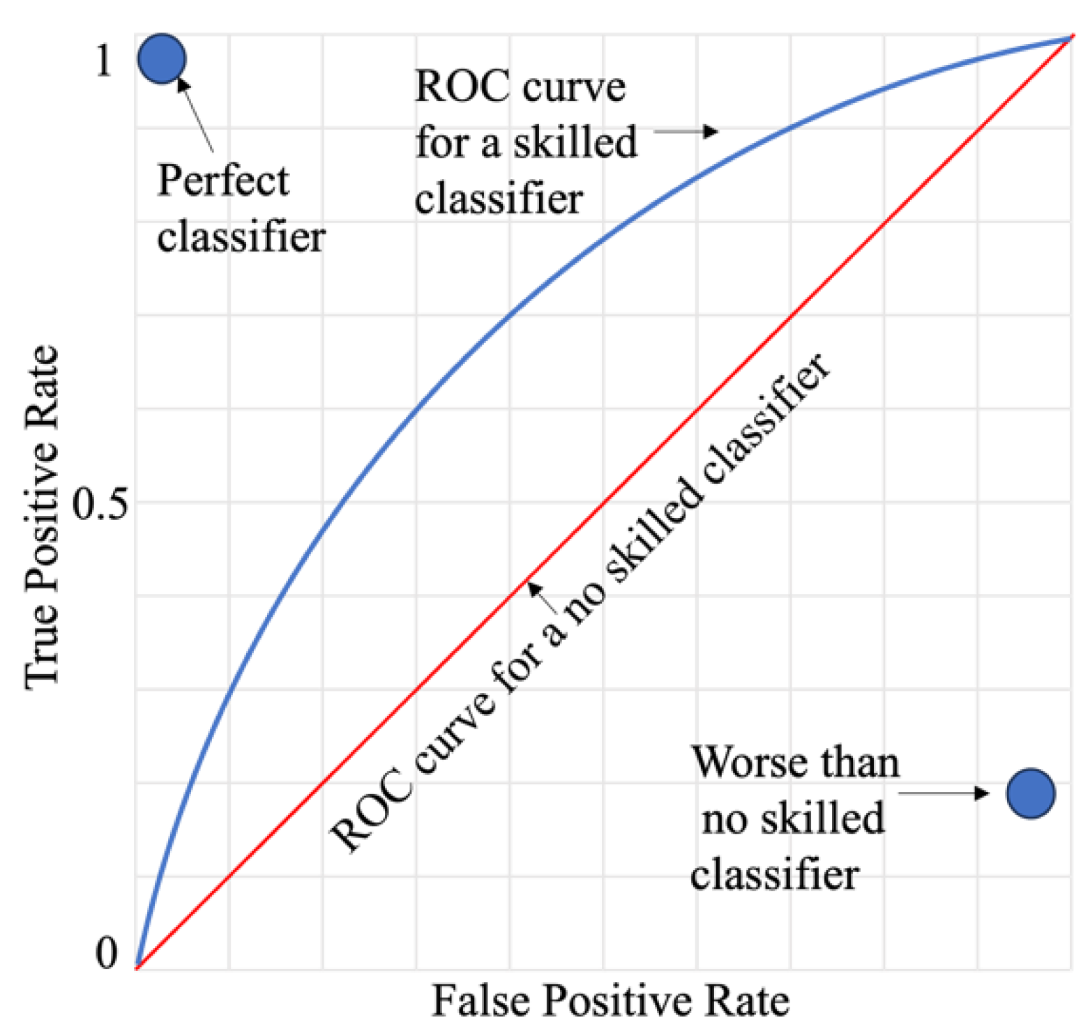
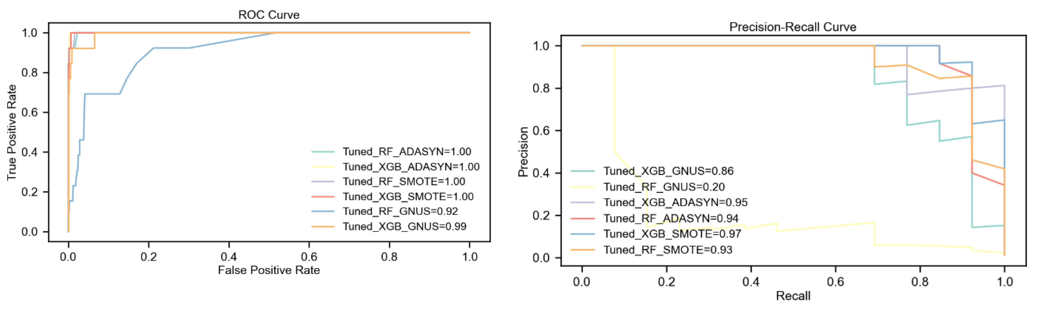
The Receiver Operating Characteristic (ROC) Curve and the Area Under the ROC Curve (ROC AUC) are pivotal metrics in churn prediction and similar fields. The ROC Curve visualizes the trade-off between the true positive rate (TPR or recall) and the false positive rate (FPR) across various classification thresholds, providing a comprehensive evaluation of a classifier's ability to distinguish between classes:
A model with no predictive ability produces a ROC curve that aligns with the diagonal line of no-discrimination, while a perfect model's ROC curve reaches the top-left corner, signifying maximum TPR and minimal FPR. The ROC AUC metric, which quantifies the area under the ROC curve, measures this performance, with values closer to 1 indicating superior model effectiveness, as depicted in
Figure 1.
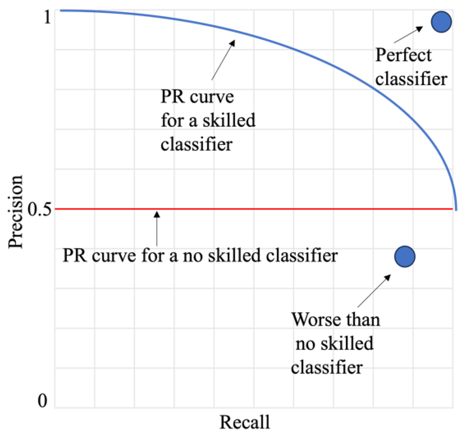
For highly imbalanced datasets, however, the Precision-Recall (PR) Curve and the Area Under the PR Curve (PR AUC) are often more informative. Unlike the ROC Curve, the PR Curve emphasizes the minority class by illustrating the trade-off between precision and recall, providing critical insights where the ROC curve might present an overly optimistic view [
75], as depicted in
Figure 2.
This paper adopts a comprehensive framework for evaluating ML models, synthesizing insights from both threshold metrics (e.g., precision, recall, and F1-score) and ranking metrics (e.g., ROC AUC and PR AUC). By integrating these perspectives, the study ensures a holistic understanding of model performance, with a particular focus on accurately predicting minority class instances and addressing the challenges of imbalanced datasets.
When evaluating multiple ML models across four datasets with varying levels of class imbalance ranging from moderate (15% churned) to extremely high imbalance (1% churned)—it is essential to use metrics that accurately reflect the models' ability to handle imbalanced data and predict minority class instances. For datasets with severe class imbalance, such as DS4 with only 1% churners, PR AUC is often a more reliable metric than ROC AUC. The key reason is that ROC AUC evaluates the model’s ability to distinguish between the positive (churn) and negative (non-churn) classes across all possible classification thresholds, considering both True Positive Rate (TPR) and False Positive Rate (FPR). However, in extreme class imbalance, the number of negative instances (non-churners) overwhelms the dataset, causing the FPR to remain low even for poorly performing models. As a result, even a model with poor precision on the minority class (churners) may still achieve a high ROC AUC score, making it an overly optimistic indicator of real-world performance.
In contrast, PR AUC focuses specifically on the minority class (churners), measuring the trade-off between precision and recall. Precision evaluates how many of the predicted churners are actually correct, while recall assesses how many of the actual churners were correctly identified. This makes PR AUC particularly useful for evaluating the effectiveness of a model in correctly predicting churners, even when their proportion is extremely low. For example, our results demonstrate that even in DS4 (1% churn rate), models achieved near-perfect ROC AUC scores (100% for some cases), but the PR AUC values were significantly lower, revealing actual differences in minority class performance.
Additionally, relying solely on ROC AUC can lead to misleading conclusions in imbalanced datasets because it does not differentiate between models that predict a large number of false positives versus models that are genuinely capable of identifying minority class instances. A classifier that predicts almost all cases as non-churners could still achieve a high ROC AUC due to the imbalance in class distribution, despite failing to provide actionable insights for churn prediction.
To address this limitation, our study follows best practices in class-imbalanced learning by incorporating both ROC AUC and PR AUC, ensuring that model evaluation captures the real impact on the minority class while maintaining an overall perspective. This distinction is particularly evident in DS4, where PR AUC results expose the performance differences between models more effectively than ROC AUC alone. The selected metrics include:
F1-Score: Combines precision and recall through their harmonic mean, offering a balanced evaluation suited for imbalanced datasets.
ROC AUC: Measures a classifier's ability to distinguish between classes across thresholds, indicating its capacity to prioritize positive over negative instances.
PR AUC: Particularly effective for extreme imbalances, focusing on minority class performance and highlighting precision-recall trade-offs.
Matthews Correlation Coefficient (MCC): Provides a balanced assessment by considering all confusion matrix elements, making it effective for datasets with significant class imbalances.
Cohen’s Kappa: Adjusts for chance agreement, offering a nuanced evaluation of classifier performance.
Given the highly imbalanced nature of the datasets, accuracy is not included as it can misrepresent model performance. In our study, churn rates range from 15% to as low as 1% (DS4), meaning that a naive model that predicts all instances as non-churners could achieve over 99% accuracy while failing to capture churners entirely. Because of this, accuracy is not a reliable measure of performance in churn prediction, as it does not reflect the model’s ability to correctly classify the minority class.
However, in a more balanced dataset (e.g., a 50-50 churn/non-churn split), accuracy could still provide meaningful insights, especially if the cost of misclassification is equal for both classes. Additionally, in preliminary model evaluations, accuracy may serve as a baseline measure before incorporating techniques that handle imbalance more effectively. Despite these cases, best practices in imbalanced classification recommend F1-Score, ROC AUC, PR AUC, Cohen’s Kappa, and MCC, as they provide a more reliable assessment of a model’s ability to distinguish churners from non-churners.
By excluding accuracy, our study aligns with these best practices to ensure that performance evaluations focus on the model’s effectiveness in handling class imbalance rather than simply optimizing for majority-class predictions. Precision and recall are also excluded as standalone metrics since their combined effect is adequately captured by the F1-Score. This evaluation framework—comprising F1-Score, ROC AUC, PR AUC, MCC, and Cohen’s Kappa—ensures a comprehensive assessment of both overall model accuracy and the ability to identify rare events, such as customer churn, in imbalanced datasets.
3. Datasets
3.1. Data Description
In the scope of this investigation, four datasets from publicly accessible sources were utilized, hereinafter referred to as Ds1, DS2, DS3, and DS4. Dataset 1 was sourced from the Kaggle platform [
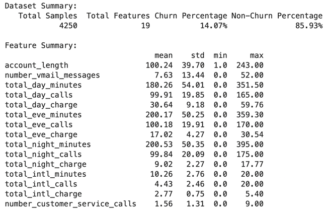
76] and encompasses 4,250 records alongside 20 attributes, as described in the below tables. This dataset is characterized by its heterogeneity, comprising both categorical and numerical types of data; specifically, it includes 15 numerical attributes and 5 categorical attributes. The content of the dataset encompasses a wide range of customer information, such as demographic details, service subscriptions (e.g., contract duration), technical support interactions, and financial transactions (e.g., total charges incurred by the customer). The distribution of the classes within this dataset reveals a churn to non-churn ratio of 1:7, with the churn category constituting approximately 15% of the data.
Datasets 2, 3, and 4 are produced from dataset 1 to have datasets with different level of imbalance rates. We used KMeans algorithm to remove number of instances in the minority class and create a dataset with 90% non-churned and 10% churned as DS2, 95% non-churned and 5% churned as DS3, and 99% non-churned and 1% churned as DS4.
Table 2.
The names and types of different variables in the churn dataset.
Table 2.
The names and types of different variables in the churn dataset.
| Variable Name (Meaning) |
Type |
| state, (the US state of customers) |
string |
| account_length (number of active months) |
numerical |
| area_code, (area code of customers) |
string |
| international_plan, (whether customers have international plans) |
yes/no |
| voice_mail_plan, (whether customers have voice mail plans) |
yes/no |
| number_vmail_messages, (number of voice-mail messages) |
numerical |
| total_day_minutes, (total minutes of day calls) |
numerical |
| total_day_calls, (total number of day calls) |
numerical |
| total_day_charge, (total charge of day calls) |
numerical |
| total_eve_minutes, (total minutes of evening calls) |
numerical |
| total_eve_calls, (total number of evening calls) |
numerical |
| total_eve_charge, (total charge of evening calls) |
numerical |
| total_night_minutes, (total minutes of night calls) |
numerical |
| total_night_calls, (total number of night calls) |
numerical |
| total_night_charge, (total charge of night calls) |
numerical |
| total_intl_minutes, (total minutes of international calls) |
numerical |
| total_intl_calls, (total number of international calls) |
numerical |
| total_intl_charge, (total charge of international calls) |
numerical |
| number_customer_service_calls, (number of calls to customer service) |
numerical |
| churn, (customer churn—the target variable) |
yes/no |
Table 3.
Dataset summary.
Table 3.
Dataset summary.
3.2. Data Preprocessing
The data preprocessing journey begins with a rigorous approach to removing outliers, a crucial step in ensuring the dataset's robustness and reliability. A custom-designed function, aptly named remove_outliers, takes center stage in this process. This function operates systematically, meticulously analyzing each specified feature in the dataset to identify and mitigate the impact of extreme values.
The process starts by calculating the first (Q1) and third quartiles (Q3) for each feature. These quartiles, representing the 25th and 75th percentiles, respectively, provide a snapshot of the data's central tendency and spread. From these values, the interquartile range (IQR) is determined, encapsulating the middle 50% of the data. The IQR serves as the benchmark for identifying outliers, as it forms the basis for establishing upper and lower bounds. The upper bound is set as , while the lower bound is defined as . Any data points falling outside these bounds are flagged as outliers. Once identified, these outliers are addressed thoughtfully. Instead of removing them, the function replaces their values with the feature’s median, a robust measure of central tendency that is less influenced by extreme values. This approach neutralizes the outliers' impact while preserving the dataset's integrity, ensuring no valuable information is lost. With all features processed, the function returns a refined dataset, primed for accurate and reliable analysis.
The next phase involves handling categorical variables, transforming them into numerical representations suitable for machine learning models. The process begins with specific columns, such as area_code, international_plan, voice_mail_plan, and churn, being mapped from their original string formats to numerical codes. For instance, area_code values are translated into their corresponding numerical identifiers (e.g., 415, 408, 510), while binary attributes like international_plan and churn are encoded as 1 for "yes" and 0 for "no." The transformation extends to the state column, which, while categorical, lacks an inherent ordinal relationship. Here, an OrdinalEncoder assigns unique integers to each state, converting it into a format compatible with machine learning algorithms. This process ensures that all categorical features are seamlessly integrated into the dataset.
The final step focuses on the normalization of numerical variables, ensuring that every feature contributes equally to the model’s performance by standardizing their scales. A subset of the dataset containing only numerical features is isolated, including the newly encoded categorical variables. To normalize these features, the MinMaxScaler from scikit-learn is applied. This scaler transforms each value to a range between [0, 1], calculated by subtracting the feature’s minimum value from the current value and dividing by the range (i.e., the difference between the maximum and minimum values). The transformed values maintain the dataset’s original distribution patterns while ensuring that all features are on a comparable scale. Formally, this is represented as:
In this formula, and represent the minimum and maximum values of the feature, respectively, while denotes the normalized value of the feature after transformation. The normalized features are then reassembled into a new pandas DataFrame, with column names preserved for clarity and consistency. This carefully processed data, now rid of outliers, encoded for numerical compatibility, and normalized for uniformity, is ready for analysis. With its structural integrity intact and its features optimized, the dataset stands as a robust foundation for the application of machine learning algorithms, ensuring accurate and meaningful insights in subsequent research.
4. Methods
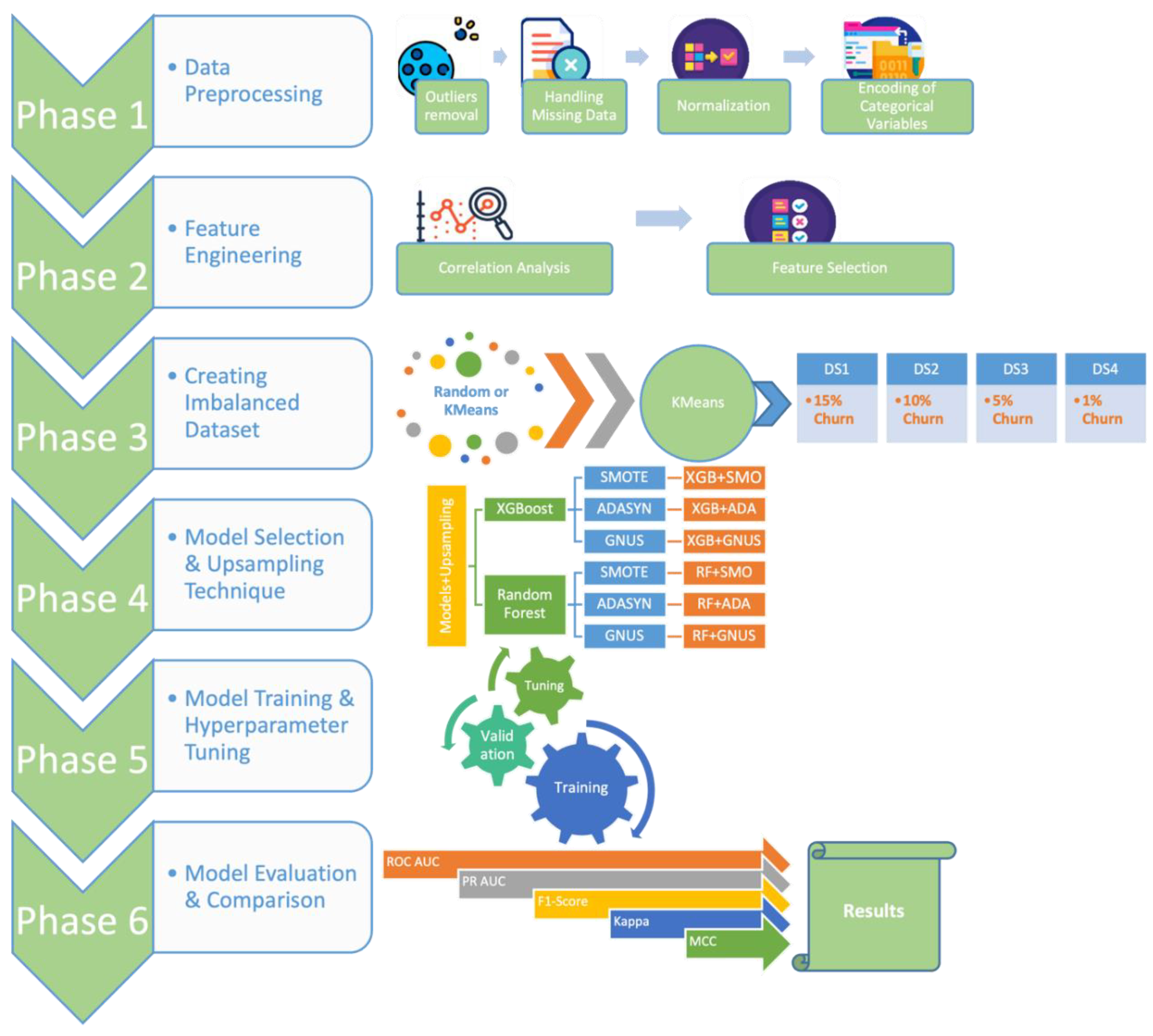
The research methodology was systematically divided into six distinct phases: data preprocessing, feature engineering, the creation of imbalanced datasets, model selection and application of upsampling techniques, model training and hyperparameter tuning, and model evaluation and comparison using unseen test data across four datasets with varying levels of imbalance, as illustrated in
Figure 3. All analyses and practical implementations were performed using the open-source programming language Python, incorporating libraries such as Numpy [
77], Pandas [
78], Matplotlib [
79], Imblearn [
80], Scikit-learn [
81], among others. The work was conducted within the Jupyter Notebook environment on an Apple MacBook Air M2 with 16 GB of RAM, ensuring a robust computational setup for the study. This computational setup provided a robust platform for managing the datasets and executing the complex data analysis and ML model development required for the study.
The study addresses two critical questions within the telecommunications domain related to customer churn prediction. The first question seeks to identify the machine learning techniques most effective for predicting customer churn in highly imbalanced datasets. The second question examines the extent to which oversampling techniques—such as SMOTE, ADASYN, and GNUS—enhance the predictive accuracy of these models. To ensure credible and generalizable results, a substantial volume of data was analyzed.
To address these questions effectively, several research strategies were considered. The primary criterion for the chosen methodology was its ability to yield reliable and accurate answers to the research questions. Ultimately, an experimental research strategy was adopted, focusing on investigating specific factors influencing customer churn prediction. These factors include various machine learning algorithms and oversampling techniques. In this experimental setup, the independent variables are the machine learning algorithms and oversampling methods, while the dependent variable is the accuracy of churn prediction.
The experimental research approach was selected for its ability to ensure reproducibility, precision, and credibility in the findings, as it systematically examines the impacts of the independent variables on the dependent variable [
82]. Given the characteristics of the data and the specificity of the techniques employed, this approach was determined to be the most suitable for the study's objectives.
4.1. Splitting Data
The datasets were partitioned into training and testing subsets, with 70% allocated for training and 30% for testing. This partitioning was performed using the stratified train-test split functionality available in Python's Scikit-learn Model Selection library. The stratified split ensures that the class distribution proportions in the original dataset are preserved in both subsets. This approach is critical for maintaining class balance, enabling the model to be trained and evaluated on data that accurately reflects the overall dataset's distribution.
Following the partitioning, the training subset underwent a 10-fold cross-validation process. This technique divides the training data into 10 equal segments, iteratively using nine folds for training and one for validation in each cycle. This comprehensive approach allows for an in-depth evaluation of model performance, helping to enhance the robustness and generalizability of the predictive models by mitigating overfitting and ensuring the model performs well across various data subsets.
In the final phase, the previously set-aside testing dataset was utilized for a thorough evaluation of the predictive capabilities of the final models. This step provided a realistic assessment of the models' performance on unseen data, offering valuable insights into their potential applicability and effectiveness in real-world scenarios.
4.2. Feature Selection
Feature engineering is a critical component in the development of machine learning (ML) models, involving the transformation and creation of new features from existing ones to optimize the feature space. The primary goal is to derive variables that can enhance model performance by providing the algorithm with more meaningful or refined inputs. This process offers several advantages, including reducing the risk of overfitting, simplifying model complexity, and conserving computational resources. While feature engineering may sometimes compromise model interpretability, it accelerates the learning process and mitigates redundant covariances among features, contributing to more robust models [
83].
In this study, feature engineering commenced with the classification of features into numerical and categorical groups based on their data types. This initial step was crucial for applying appropriate transformation and preprocessing techniques suited to each type. An in-depth correlation analysis followed, focusing specifically on the numerical features. By examining the relationships among these features, the analysis aimed to uncover potential redundancies or interdependencies that could negatively impact the models.
Special attention was given to identifying numerical features with high interdependence. Features that exhibited strong correlations with others were flagged as potentially redundant, as they might not provide unique or additional value to the models. Furthermore, such redundancies could introduce noise or unnecessary complexity, detracting from the model's overall performance. Based on this analysis, a strategic subset of features was selected for removal. The decision to eliminate these features was driven by the intent to streamline the dataset, ensuring that the remaining features contributed distinct and valuable information to the learning process.
To achieve this, the study employed a correlation matrix of the numerical features, visualized through a heatmap. This visual representation facilitated the identification of highly correlated variables, making it easier to pinpoint features for removal. By reducing the duplication of information and eliminating redundant variables, the dataset was refined to optimize its utility for ML models.
This meticulous feature engineering process resulted in a more concise and meaningful dataset. The streamlined feature set reduced complexity and enhanced the efficiency and effectiveness of the models, ultimately aiming to improve predictive accuracy. With the refined dataset, the study proceeded to the subsequent phases of model training and evaluation, laying a strong foundation for robust and high-performing ML models.
4.3. Creating Highly Imbalanced Datasets
To thoroughly evaluate the performance of our models and sampling techniques, we constructed highly imbalanced datasets derived from the existing data. This involved two distinct methodologies: a random undersampling approach and KMeans clustering. These approaches were designed to create varying levels of imbalance, providing a robust framework for testing the effectiveness of the models and sampling strategies under different conditions.
4.3.1. Random Undersampling
The random undersampling approach creates highly imbalanced datasets by selectively reducing the number of minority class instances (churn) while preserving the majority class instances (non-churn). This method replicates extreme imbalance scenarios, providing a robust framework for testing model performance under challenging conditions.
Selectively Reduce Minority Instances: A subset of the minority class is randomly selected to achieve the desired imbalance ratio. This ensures that the minority class size aligns with the targeted level of imbalance.
Maintain Majority Class: The majority class remains unchanged, ensuring that the overall dataset size is not significantly affected.
Random Sampling: The DataFrame.sample() function is used with a specified random_state to ensure reproducibility. The n parameter is adjusted to control the number of minority class instances retained.
Shuffling: After combining the reduced minority class and the unchanged majority class, the dataset is shuffled to eliminate any order-based biases that could influence the training phase.
This approach, though simple and efficient, may result in the loss of valuable information contained in the minority class. Therefore, validating the generalizability of models trained on such imbalanced datasets is crucial to ensure their applicability to real-world scenarios. This step is essential to assess whether the models can maintain their predictive performance despite the loss of some minority class information.
4.3.2. KMeans Clustering
To mitigate the drawbacks of Random Undersampling, we implemented KMeans-based clustering for minority class reduction. Instead of removing minority samples arbitrarily, this approach retains only the most representative samples, ensuring that the distribution of the minority class is better preserved.
Cluster Formation & Centroid Selection: Minority class instances are grouped into clusters using KMeans clustering, with each cluster representing a subgroup of the churners. The centroid of each cluster is retained as the most representative instance.
Preserving Informative Features: By focusing on cluster centroids, this method ensures that structural characteristics of the minority class are maintained, reducing the risk of removing critical data points.
Avoiding Redundant Data: Unlike Random Undersampling, which may eliminate important or rare churn cases, KMeans strategically selects instances that best define the minority class distribution.
Since clustering-based undersampling preserves minority class diversity while reducing dataset size, models trained on KMeans-reduced datasets consistently outperformed those trained on randomly undersampled datasets. This was particularly evident in scenarios with extreme class imbalance, where retaining meaningful minority class representations is crucial.
Unlike Random Undersampling, which removes minority class instances without considering their distribution in the feature space, KMeans clustering offers a more structured approach by retaining representative centroids that capture the core characteristics of the minority class. By selecting these centroids rather than randomly eliminating data points, this method helps preserve class separability, ensuring that the diversity within the minority class remains intact. Additionally, by maintaining a well-balanced representation, KMeans reduces the risk of overfitting to the majority class, a common issue when key churn instances are lost during random sampling. Instead of training on an arbitrarily reduced dataset, models benefit from learning on a strategically selected subset that better reflects the overall distribution of the minority class. These advantages make KMeans-based undersampling a more effective strategy for managing class imbalance in churn.
Despite its advantages, KMeans undersampling is not without limitations. A key concern is that it relies on the assumption that centroids adequately represent the minority class distribution. If the minority class contains high variability or rare subgroups, centroid-based selection may oversimplify the data, potentially introducing bias by failing to retain underrepresented patterns.
Additionally, the effectiveness of this approach depends on the number of clusters chosen. Setting too few clusters risks oversimplifying the minority class, while too many clusters reduce the efficiency of undersampling, leading to minimal dataset size reduction. Future work could explore adaptive clustering techniques that dynamically determine the optimal number of clusters based on data complexity
4.4. Class Imbalance
In churn prediction, datasets often exhibit significant class imbalances, stemming from the relatively lower incidence of customer churn compared to those who continue using services. This imbalance creates a critical challenge for ML models, which tend to favor the majority class, thereby neglecting the minority class. Such bias undermines predictive accuracy, particularly in detecting churn, which is typically the primary focus. In this study, the datasets revealed notable class imbalances, with churn rates of approximately 15% in dataset 1, 10% in dataset 2, 5% in dataset 3, and as low as 1% in dataset 4.
To address this issue, the study employed a strategic approach utilizing three advanced oversampling techniques: SMOTE, ADASYN, and GNUS. These methods are designed to augment the representation of the minority class, thereby creating a more balanced dataset for training. By increasing the presence of churn instances, these techniques enhance the model's ability to learn patterns associated with customer churn, mitigating the adverse effects of class imbalance.
A pivotal element in implementing these oversampling techniques was their restriction to the training dataset within the context of 10-fold cross-validation. This strategy involved applying oversampling exclusively to nine of the folds while reserving the tenth fold for evaluation. This careful segmentation ensures that the evaluation data remains unaltered, avoiding inflated performance estimates that could arise from oversampling being applied indiscriminately across the entire dataset. By confining oversampling to the training phase, the study minimized the risk of overfitting and ensured a more realistic and generalizable assessment of model performance.
This deliberate and methodical approach underscores the importance of addressing class imbalance in churn prediction datasets. By integrating oversampling techniques into the cross-validation framework, the study aimed to develop ML models that are both robust and sensitive to the intricacies of churn behavior, ultimately contributing to more accurate and reliable predictive performance.
5. Results and Discussion
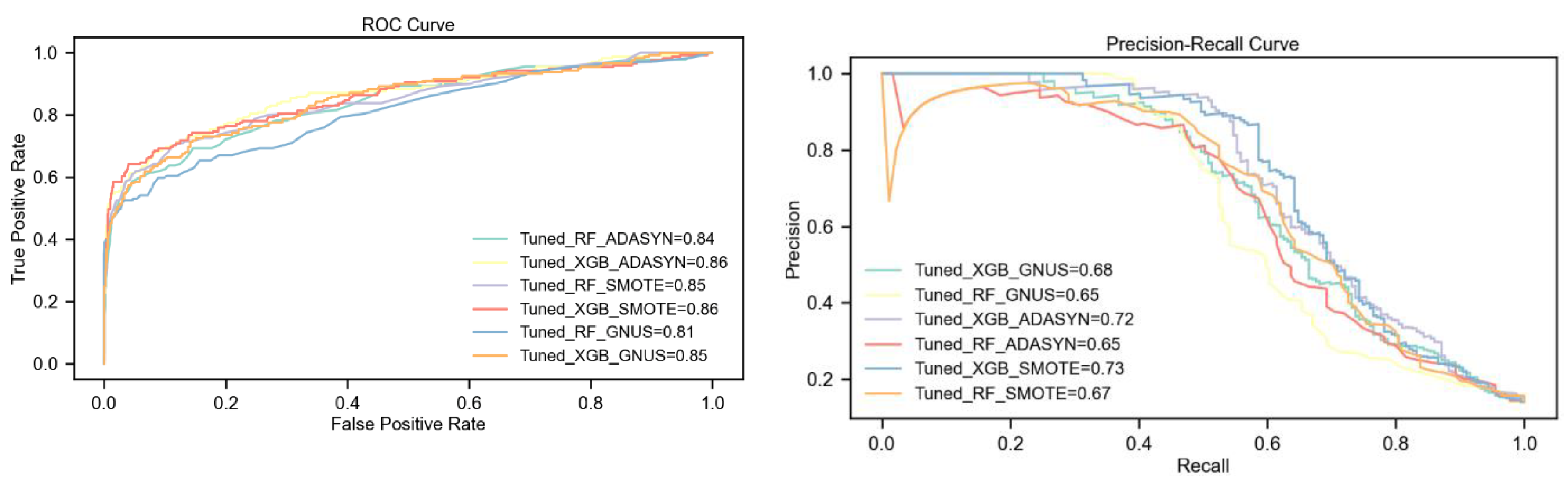
5.1. Results on DS1 with 15% Churn Ratio
The evaluation shows that the tuned XGBoost model consistently outperforms Random Forest, particularly when paired with the SMOTE upsampling technique. Under SMOTE, XGBoost achieves the highest scores across all key metrics, including a 4% higher F1-Score, a 6% higher PR-AUC, and notable improvements in Kappa and MCC (5% and 4%, respectively). This demonstrates the strong synergy between XGBoost's advanced learning capabilities and SMOTE's synthetic sample generation.
Using ADASYN, XGBoost shows moderate improvements over Random Forest, with a 1% higher F1-Score and a significant 7% advantage in PR-AUC, though both models exhibit similar Kappa statistics. GNUS is the least effective upsampling method, with both models performing equally in F1-Score and Kappa, but XGBoost still maintains modest gains in ROC-AUC (4%) and PR-AUC (3%).
Overall, SMOTE-enhanced XGBoost delivers the best performance, significantly surpassing ADASYN and GNUS in addressing class imbalance. These findings, detailed in
Table 4 and
Figure 4, affirm SMOTE as the most effective technique and XGBoost as the most robust model for this dataset.
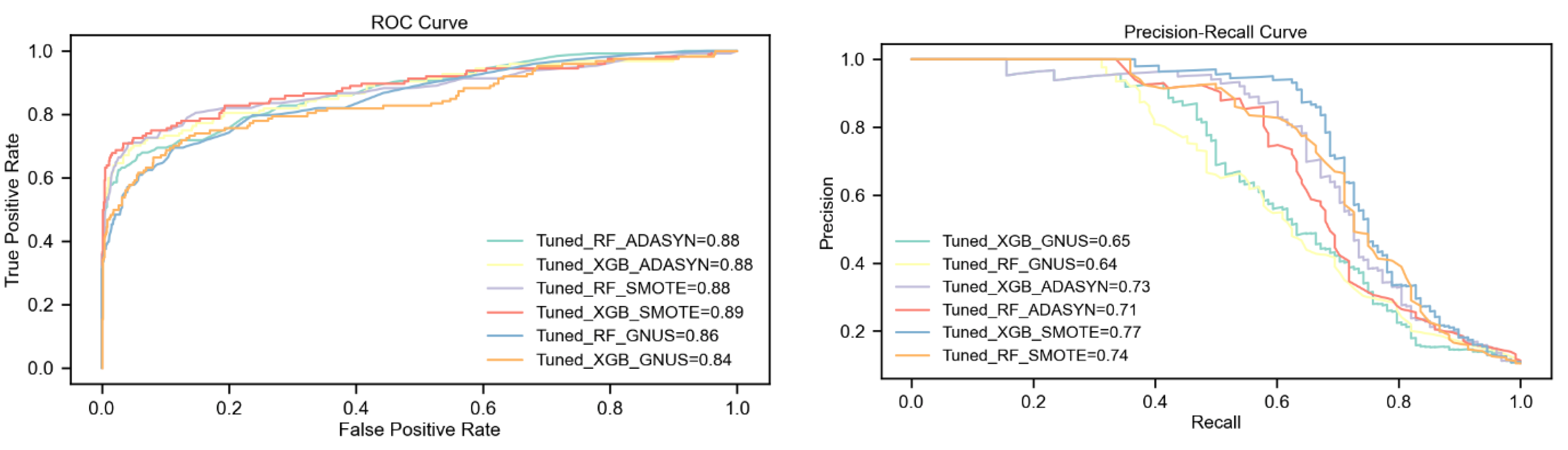
5.2. Results on DS2 with 10% Churn Ratio
The analysis reveals that the tuned XGBoost model paired with SMOTE consistently achieves the highest performance across all metrics, including F1-Score, PR-AUC, Kappa, and MCC. SMOTE proves to be the most effective upsampling method, enabling XGBoost to significantly outperform Random Forest, particularly with a 7% higher F1-Score and 8% higher Kappa statistic.
With ADASYN, XGBoost maintains an advantage, achieving a 3% higher F1-Score and a slight improvement in PR-AUC over Random Forest. However, both models show equal ROC-AUC performance under this technique. GNUS, by contrast, favors Random Forest, which outperforms XGBoost in most metrics, highlighting GNUS's limited compatibility with XGBoost.
Overall, SMOTE-enhanced XGBoost emerges as the optimal approach for addressing class imbalance, consistently delivering the best results, as summarized in
Table 5 and illustrated in
Figure 5.
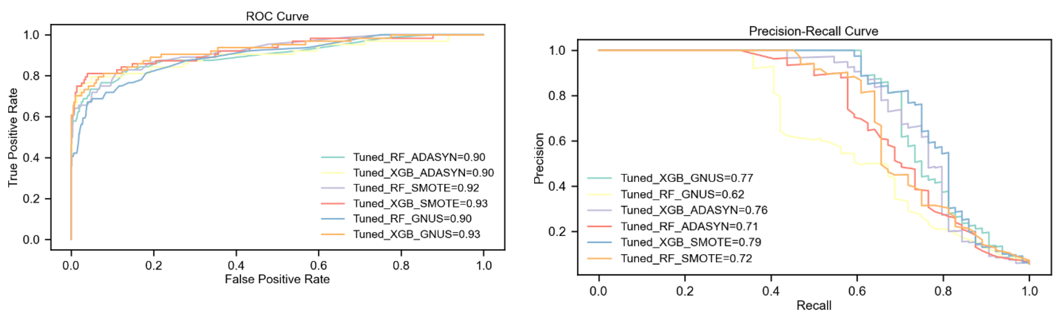
5.3. Results on DS3 with 5% Churn Ratio
The analysis highlights the consistent superiority of the tuned XGBoost model over Random Forest across all upsampling techniques, particularly with SMOTE. Under SMOTE, XGBoost achieves the highest overall performance, including a 5% higher F1-Score (75%), a 7% higher PR-AUC (79%), and significant gains in Kappa and MCC (6% and 5%, respectively). This combination demonstrates the strong synergy between XGBoost's advanced learning capabilities and SMOTE's ability to generate effective synthetic samples.
With ADASYN, XGBoost outperforms Random Forest by 5% in F1-Score and PR-AUC, while both models achieve an equal ROC-AUC of 90%. Additionally, XGBoost shows notable improvements of 6% in Kappa and MCC, reflecting its stronger predictive reliability. GNUS reveals the largest performance gap, where XGBoost outshines Random Forest with an 11% higher F1-Score, a 15% improvement in PR-AUC, and double-digit gains in Kappa and MCC.
Overall, SMOTE emerges as the most effective upsampling technique, delivering the best results for both models, especially XGBoost. While ADASYN provides moderate benefits, GNUS proves less effective overall, though XGBoost demonstrates remarkable resilience under this technique. The combination of tuned XGBoost with SMOTE achieves the highest scores across all metrics, affirming its robustness and suitability for handling extreme class imbalance. Results are detailed in
Table 6 and illustrated in
Figure 6.
5.4. Results on DS4 with 1% Churn Ratio
The evaluation highlights the tuned XGBoost model's remarkable superiority over Random Forest across all upsampling techniques, particularly in scenarios of extreme class imbalance. With ADASYN, XGBoost achieves significantly higher F1-Score and Kappa (80% vs. 47%) and a substantial 25-point advantage in MCC (80% vs. 55%), despite both models achieving a perfect ROC AUC of 100%. XGBoost also demonstrates a slight edge in PR AUC, scoring 95% compared to Random Forest's 94%.
SMOTE further amplifies the performance gap, with XGBoost reaching an F1-Score and Kappa of 92%, outperforming Random Forest by 36%. XGBoost also surpasses Random Forest in PR AUC by 4% (97% vs. 93%) and MCC by 30 points (92% vs. 62%), while maintaining a perfect ROC AUC of 100%. These results confirm the effectiveness of combining SMOTE with XGBoost in handling extreme class imbalance.
The largest performance differences emerge with GNUS. XGBoost achieves an F1-Score of 74%, 47% higher than Random Forest, and a PR AUC of 86%, vastly outperforming Random Forest's 20%. XGBoost also achieves a 41-point lead in MCC (74% vs. 33%) and a 7% higher ROC AUC (99% vs. 92%). These findings highlight XGBoost’s robustness, even under less effective upsampling methods like GNUS.
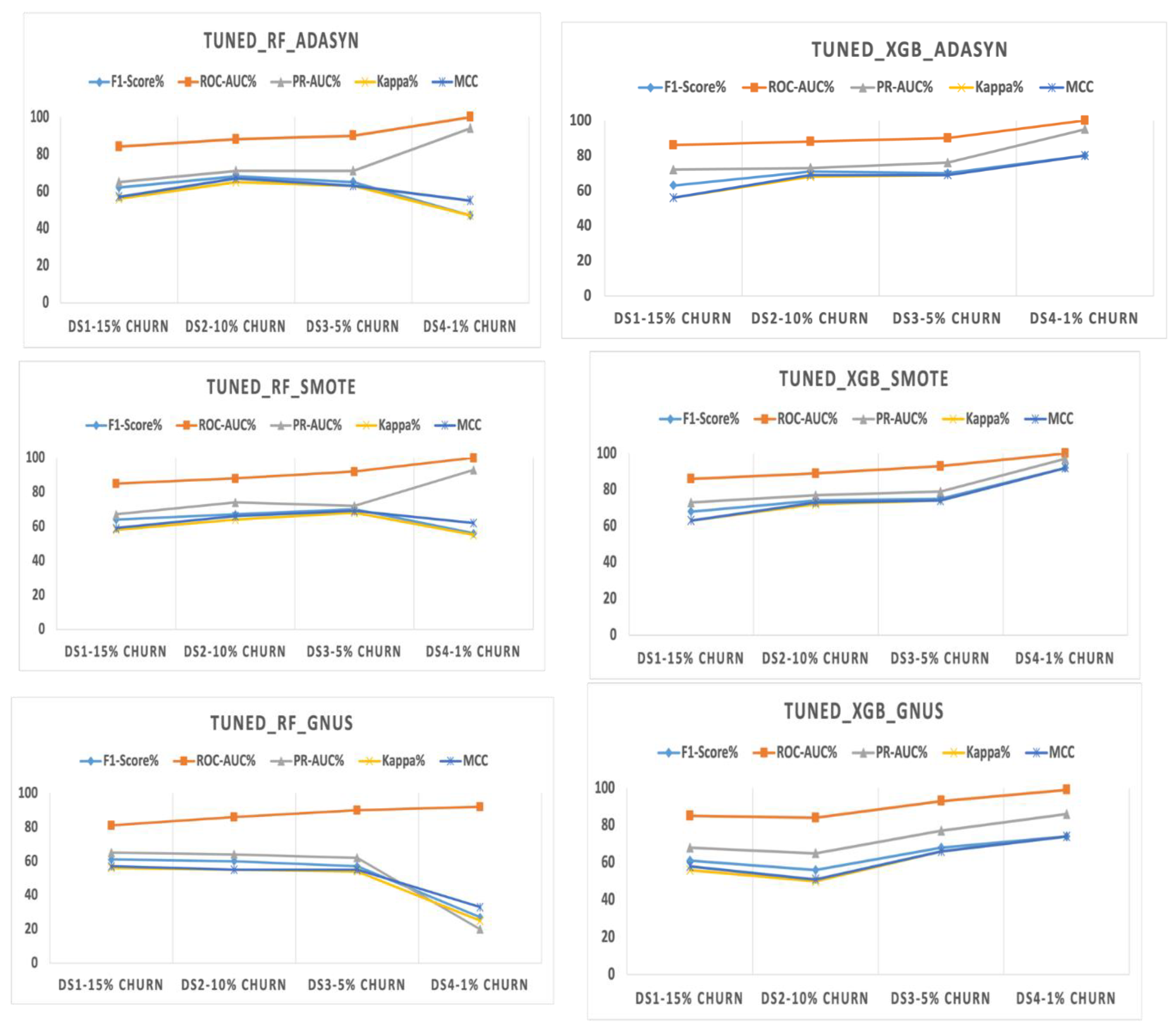
The results demonstrate that MCC and Kappa exhibit different sensitivity to extreme class imbalance depending on the model and resampling technique. While it is often assumed that MCC fluctuates more than Kappa, our experiments show that this depends on the specific model and dataset. For instance, in Tuned_RF_GNUS, MCC exhibits greater fluctuation in DS4 (1% churn), dropping from 55 to 33, while Kappa drops from 54 to 25. This aligns with MCC’s formulation, which is highly sensitive to class distribution distortions when the minority class becomes extremely small. However, in other models, such as Tuned_RF_ADASYN and Tuned_RF_SMOTE, Kappa fluctuates more than MCC, indicating that MCC is not universally more volatile. These findings suggest that the impact of imbalance on evaluation metrics is model-dependent, and both metrics must be interpreted carefully when dealing with extreme class imbalance.
Overall, SMOTE-enhanced XGBoost delivers the highest performance across all metrics, establishing itself as the most effective strategy for this dataset with a 1% churn rate. While ADASYN provides moderate improvements for XGBoost, it yields far lower results for Random Forest. GNUS is the least effective for Random Forest, but XGBoost consistently demonstrates resilience. The results, presented in
Table 7 and
Figure 7, emphasize the critical importance of pairing advanced models like XGBoost with effective upsampling techniques to address extreme class imbalance.
5.5. Analysis of Average Performance and Variability
Table 8 and
Table 9 provide a comprehensive analysis of the effectiveness and consistency of various machine learning models and upsampling techniques applied to datasets with differing churn ratios. These results reveal distinct patterns in both performance and variability, facilitating the identification of the most robust strategies for managing imbalanced datasets.
The data in
Table 8 highlights significant differences in model performance across various evaluation metrics. Tuned_XGB_SMOTE consistently achieves the highest average scores among all models, indicating superior effectiveness in handling imbalanced datasets with different churn ratios. Specifically, it attains the highest average F1-Score (77.25%), ROC-AUC (92.0%), PR-AUC (81.5%), Kappa (75.25%), and MCC (75.5%). This suggests that combining the XGBoost classifier with the SMOTE upsampling technique yields the most robust predictive performance.
In contrast, Tuned_RF_GNUS exhibits the lowest average performance across all metrics, with an average F1-Score of 51.25% and PR-AUC of 52.75%, indicating limited effectiveness in addressing class imbalance when using the Random Forest model with the GNUS upsampling method.
The other models, such as Tuned_XGB_ADASYN and Tuned_RF_SMOTE, show moderate performance, with Tuned_XGB_ADASYN being the second-best performer. This model achieves an average F1-Score of 71.0% and an average Kappa of 68.25%, suggesting that the XGBoost model combined with the ADASYN technique is also effective but less so than when paired with SMOTE.
Overall, the analysis underscores the importance of selecting appropriate combinations of machine learning algorithms and upsampling techniques. The superior performance of Tuned_XGB_SMOTE highlights its suitability as a robust strategy for managing imbalanced datasets, particularly in scenarios where predictive accuracy and reliability are critical.
The standard deviation is a key statistical measure that quantifies the extent of variation or dispersion within a numerical dataset. It reflects the average distance of individual data points from the dataset's mean, offering valuable insight into the overall variability of the data.
The calculation of standard deviation serves several important purposes in the context of machine learning model evaluation:
Assessing Consistency: Standard deviation helps gauge how consistently a model performs across different datasets by measuring the variability in its performance metrics.
Comparing Stability: Models with lower standard deviations exhibit more stable performance, indicating their reliability across varying datasets.
Identifying Variability: A high standard deviation reveals significant variability in model performance, which could be attributed to dataset characteristics or the sensitivity of the model to specific features or configurations.
This metric plays a critical role in understanding and comparing the robustness of machine learning models in diverse scenarios. The Standard Deviation is as follows:
: Sample standard deviation.
: Each individual data point in your dataset.
: The sample mean (average of your data points).
: The total number of data points in your sample.
: Degrees of freedom. Subtracting 1 accounts for the fact that we're estimating the population standard deviation from a sample.
Using the same methodology, we computed the standard deviations for all models and performance metrics. The results are summarized in the table below, providing a comprehensive view of the variability in model performance across different datasets. This table highlights the consistency and stability of each model, offering insights into their robustness and reliability.
XGBoost emerges as the most effective model overall, consistently outperforming Random Forest in both average metrics and adaptability. Among the configurations, XGBoost combined with SMOTE demonstrated the highest average performance across all datasets, achieving exceptional scores such as an F1-Score of 77.25% and a PR-AUC of 81.5%. This combination excelled at balancing precision and recall while maintaining strong reliability in predictions, as reflected in its high Kappa and MCC values. The slightly higher average ROC-AUC of 92.0% further reinforced its superior ability to distinguish between churners and non-churners. However, this strong performance came with notable variability, particularly in metrics like F1-Score and Kappa, indicating sensitivity to the degree of class imbalance.
When paired with ADASYN, XGBoost also delivered impressive results, with an average F1-Score of 71.0% and PR-AUC of 79.0%. Although slightly less effective than SMOTE, ADASYN provided more consistent outcomes, as evidenced by its lower standard deviations. This stability suggests that ADASYN's approach to generating synthetic samples creates reliable improvements across datasets with varying churn rates.
In contrast, the GNUS upsampling technique proved to be less effective for both models, though XGBoost managed to perform reasonably well, with an average F1-Score of 64.75% and PR-AUC of 74.0%. Random Forest struggled the most with GNUS, achieving an average F1-Score of only 51.25% and a PR-AUC of 52.75%. These results indicate that GNUS was insufficient in generating the diversity and representativeness needed to enhance learning from the minority class, particularly for Random Forest. Furthermore, GNUS exhibited the highest variability in performance metrics, such as PR-AUC and F1-Score, underscoring its inconsistency across datasets.
Random Forest's performance was comparatively more stable when combined with SMOTE or ADASYN. SMOTE helped Random Forest achieve better average metrics, such as an F1-Score of 64.25% and a PR-AUC of 76.5%. However, even in this configuration, it fell short of XGBoost’s performance, highlighting the limitations of Random Forest in handling complex class imbalance scenarios. The relatively low variability in Random Forest’s results with SMOTE indicates that it benefited from the upsampling technique’s ability to generate more representative minority class samples, albeit with less overall effectiveness than XGBoost.
The standard deviations further illuminate these trends, revealing that XGBoost with SMOTE, while achieving the best average performance, exhibited greater variability, particularly under extreme imbalance conditions. This variability suggests that the model’s performance is highly dynamic, with significant gains in challenging scenarios. By contrast, XGBoost with ADASYN delivered more consistent but slightly lower performance, making it a reliable alternative for cases where stability is prioritized.
The contrast between the models is particularly striking in their ability to handle GNUS. Random Forest showed significant declines in performance and higher variability, reflecting its inability to generalize effectively from GNUS-generated samples. On the other hand, XGBoost demonstrated adaptability, leveraging even the limited benefits of GNUS to achieve better predictions, though not at the levels seen with SMOTE or ADASYN.
In summary, the analysis highlights the clear advantage of XGBoost in handling imbalanced datasets, especially when paired with SMOTE. While SMOTE provided the highest overall performance, ADASYN emerged as a more stable alternative. GNUS, on the other hand, proved less effective and highly variable, particularly for Random Forest. These findings emphasize the importance of selecting the right combination of model and upsampling technique to address class imbalance effectively. The consistent superiority of XGBoost, combined with its adaptability to challenging conditions, underscores its value as a robust solution for predictive modeling in imbalanced scenarios.
5.6. Statistical Tests
In our investigation, we embarked on a comprehensive comparison of six models evaluated across four distinct datasets and measured by five different performance metrics. To discern whether the differences we observed were truly reflective of each model’s performance—or merely artifacts of chance—we embraced a non-parametric approach, beginning with the Friedman test. This test was particularly appealing because it is well-suited for scenarios where more than two algorithms are compared, such as our case, where we explored various combinations of Random Forest and XGBoost, each paired with different upsampling methods [
84,
85].
5.6.1. Friedman Test
Given that each model was evaluated across the same four datasets, their results were inherently correlated. Consequently, the Friedman test was chosen as the most appropriate method, as it effectively accounts for repeated-measures designs. Moreover, our chosen performance metrics—F1-score, ROC-AUC, PR-AUC, Cohen’s Kappa, and MCC—do not always conform to a normal distribution, especially given the limited number of datasets at our disposal. This non-parametric, rank-based procedure thus offered a robust alternative to more traditional methods that assume normality and homogeneity of variances.
Our analysis unfolded as a systematic narrative. We began by selecting a specific metric, say the F1-score, and organizing the data into a table that represented the performance of each model across the four datasets. For each dataset, we assigned ranks to the models, with a rank of 1 indicating the best performance and a rank of 6 representing the poorest. With these rankings in hand, we computed the average rank for each model and derived the Friedman statistic, which in turn yielded a p-value to indicate whether any model consistently outperformed the rest.
When the Friedman test revealed a significant overall difference (p < 0.05), we proceeded with the Nemenyi post-hoc test. This step allowed us to delve deeper, comparing each pair of models to pinpoint where the significant differences lay. By following this rigorous workflow for each metric, we ensured that our conclusions about model performance were based on statistically sound evidence rather than on mere chance.
In summary, our methodical use of the Friedman and Nemenyi tests provided a clear, data-driven narrative that allowed us to confidently interpret the performance differences observed across multiple datasets. This approach not only highlights the strengths and weaknesses of each model but also reinforces the reliability of our conclusions regarding their comparative effectiveness. The Friedman test statistic is computed using the following mathematical formulation:
Given:
Degrees of freedom = .
The resulting statistic is approximately distributed as a Chi-square () for moderate N.
The table below presents the F1-score rankings for each model across the datasets, where the best performance is assigned a rank of 1. It is important to note that in DS3, a tie occurred between Tuned_XGB_ADASYN (70) and Tuned_RF_SMOTE (70), with each receiving a rank of 2.5. Similarly, in DS1, a tie between Tuned_RF_GNUS (61) and Tuned_XGB_GNUS (61) resulted in both models being assigned a rank of 5.5.
Table 10.
Ranking F1-score per Dataset (Best = rank 1).
Table 10.
Ranking F1-score per Dataset (Best = rank 1).
| Models/Datasets |
DS1 |
DS2 |
DS3 |
DS4 |
| Tuned_RF_ADASYN |
4 |
3 |
5 |
5 |
| Tuned_XGB_ADASYN |
3 |
2 |
2.5 |
2 |
| Tuned_RF_SMOTE |
2 |
4 |
2.5 |
4 |
| Tuned_XGB_SMOTE |
1 |
1 |
1 |
1 |
| Tuned_RF_GNUS |
5.5 |
5 |
6 |
6 |
| Tuned_XGB_GNUS |
5.5 |
6 |
4 |
3 |
Subsequently, we computed both the sum and the average of the ranks. For instance, consider the model Tuned_RF_ADASYN evaluated on the F1-score metric across four datasets. The ranks obtained were 4, 3, 5, and 5, which sum to 17, resulting in an average rank of 4.25. Employing this same procedure, we calculated the average ranks for all other metrics and models across the four datasets, as summarized in the table below:
Table 11.
The average ranks for all other metrics and models across the four datasets.
Table 11.
The average ranks for all other metrics and models across the four datasets.
| |
Average Ranks (from the Friedman Step) |
| Models/Metrics |
F1-Score |
PR-AUC |
Kappa |
MCC |
| Tuned_RF_ADASYN |
4.25 |
4.375 |
4.375 |
4.375 |
| Tuned_XGB_ADASYN |
2.375 |
2.5 |
2.625 |
3.125 |
| Tuned_RF_SMOTE |
3.125 |
3.5 |
3 |
2.875 |
| Tuned_XGB_SMOTE |
1 |
1 |
1 |
1 |
| Tuned_RF_GNUS |
5.625 |
5.875 |
5.375 |
5.375 |
| Tuned_XGB_GNUS |
4.625 |
3.75 |
4.625 |
4.25 |
Now in this step we calculate Friedman Statistic result for F1-score based on above formula:
Degrees of freedom = 5 (since ).
We computed the Friedman test statistic (=16.0) with five degrees of freedom—reflecting the number of models minus one—and compared it to the Chi-square distribution. The value of 16.0 lies between the critical values for p=0.01 and p=0.005 for five degrees of freedom, indicating a p-value between these thresholds. Further refinement using statistical software yielded an approximate p-value of 0.007. This result implies that the likelihood of observing such a statistic by chance is below 1%, thereby providing sufficient evidence to reject the null hypothesis at the 5% significance level. Using the same procedure, we derived the Friedman test outcomes and corresponding approximate p-values for all metrics, as summarized in the table below:
As illustrated in the table above, the Friedman test reveals statistically significant differences among the six models for F1, PR-AUC, Kappa, and MCC at the 5% level. In contrast, the ROC-AUC metric does not reach significance (p ≈ 0.08), leading us to retain the null hypothesis for this measure. Consequently, a post-hoc analysis will be conducted to identify the specific model differences for the metrics that exhibit overall significance.
5.6.2. Post-Hoc Analysis
This section provides an overview of our post-hoc analysis utilizing the Nemenyi test, which was conducted on the metrics that exhibited significant differences in the Friedman test. The analysis begins by ranking the models on each dataset—assigning a rank of 1 for the best performance and 6 for the worst. We then compute the average rank for each model across all datasets. Next, we calculate the Critical Difference (CD) at a significance level of
. For
models and
datasets, the CD for Nemenyi is given by:
where
represents the critical value from the Studentized range distribution for k groups at the chosen significance level
,
is the number of models, and
is the number of datasets. Finally, we compare the absolute differences in average ranks between each pair of models to the CD; if for model
and model
then the difference meets or exceeds the CD, the pair is considered significantly different at
. For our analysis, with six models and four datasets, the approximate CD is 3.80.
By applying the Nemenyi post-hoc procedure to the results presented in
Table 12, we observed that, among the evaluated metrics—F1-score, PR-AUC, Cohen’s Kappa, and MCC—only the comparison between Tuned_XGB_SMOTE and Tuned_RF_GNUS yielded a critical difference (CD) of 3.8 or greater. In essence, for every metric where the Friedman test signaled statistically significant differences (with the exception of ROC-AUC), the only pair of models that demonstrated a statistically significant difference at the conventional α = 0.05 level was that between Tuned_XGB_SMOTE and Tuned_RF_GNUS.
Although the comparisons between Tuned_XGB_SMOTE and both Tuned_XGB_GNUS and Tuned_RF_ADASYN approached the critical difference threshold (CD ≈ 3.80), they ultimately did not meet the criteria for significance. Under the strict binary decision rule of the Nemenyi test, these pairs are formally deemed non-significant, even though their proximity to the threshold suggests a potential trend favoring Tuned_XGB_SMOTE.
In terms of model performance, Tuned_XGB_SMOTE frequently achieved the highest average ranks across the datasets, establishing it as the dominant model. However, given our limited sample of four datasets, it was only statistically superior to Tuned_RF_GNUS. Conversely, Tuned_RF_GNUS consistently ranked near the bottom, and the post-hoc analysis confirmed that its performance gap with Tuned_XGB_SMOTE was indeed significant.
It is important to acknowledge that the relatively small number of datasets contributes to a larger critical difference, and with a larger sample size, additional significant differences might emerge. Moreover, while this study focuses on customer churn prediction—a domain that, although important, may not be as critical as sectors such as healthcare or finance—we have adhered to the conventional significance level of α = 0.05. For applications in industries with higher stakes, such as healthcare, it may be prudent to recalculate the significance using a more stringent threshold (e.g., α = 0.01 or α = 0.001) to mitigate the risk of false positives that could result in costly or unsafe outcomes.
5.7. Overall Comparison and Analysis
The results presented in the below Table and Figure provide valuable insights into the performance and reliability of different machine learning models and upsampling techniques across datasets with churn ratios ranging from 15% to 1%.
Table 13.
The summary of all models' performance on four datasets.
Table 13.
The summary of all models' performance on four datasets.
| Models/Metrics |
F1-Score% |
ROC-AUC% |
PR-AUC% |
Kappa% |
MCC% |
F1-Score% |
ROC-AUC% |
PR-AUC% |
Kappa% |
MCC% |
| |
DS 1 (15% churn) |
DS 2 (10% churn) |
| Tuned_RF_ADASYN |
62 |
84 |
65 |
56 |
57 |
68 |
88 |
71 |
65 |
67 |
| Tuned_XGB_ADASYN |
63 |
86 |
72 |
56 |
56 |
71 |
88 |
73 |
68 |
69 |
| Tuned_RF_SMOTE |
64 |
85 |
67 |
58 |
59 |
67 |
88 |
74 |
64 |
66 |
| Tuned_XGB_SMOTE |
68 |
86 |
73 |
63 |
63 |
74 |
89 |
77 |
72 |
73 |
| Tuned_RF_GNUS |
61 |
81 |
65 |
56 |
57 |
60 |
86 |
64 |
55 |
55 |
| Tuned_XGB_GNUS |
61 |
85 |
68 |
56 |
58 |
56 |
84 |
65 |
50 |
51 |
| |
DS 3 (5% churn) |
DS 4 (1% churn) |
| Tuned_RF_ADASYN |
65 |
90 |
71 |
63 |
63 |
47 |
100 |
94 |
47 |
55 |
| Tuned_XGB_ADASYN |
70 |
90 |
76 |
69 |
69 |
80 |
100 |
95 |
80 |
80 |
| Tuned_RF_SMOTE |
70 |
92 |
72 |
68 |
69 |
56 |
100 |
93 |
55 |
62 |
| Tuned_XGB_SMOTE |
75 |
93 |
79 |
74 |
74 |
92 |
100 |
97 |
92 |
92 |
| Tuned_RF_GNUS |
57 |
90 |
62 |
54 |
55 |
27 |
92 |
20 |
25 |
33 |
| Tuned_XGB_GNUS |
68 |
93 |
77 |
66 |
66 |
74 |
99 |
86 |
74 |
74 |
Figure 8.
The performance of the models with upsampling techniques on datasets with different levels of imbalance.
Figure 8.
The performance of the models with upsampling techniques on datasets with different levels of imbalance.
The evaluation of machine learning models and upsampling techniques across datasets with varying churn rates provides valuable insights into addressing class imbalance. By analyzing Random Forest and XGBoost models paired with SMOTE, ADASYN, and GNUS across datasets with churn rates of 15%, 10%, 5%, and 1%, this study sheds light on how model performance evolves under increasing imbalance. Key performance metrics such as F1-Score, ROC-AUC, PR-AUC, Kappa, and MCC were examined to reveal critical patterns.
When ADASYN was applied, XGBoost demonstrated a remarkable ability to maintain and even enhance its performance as churn rates decreased. For example, in the dataset with a 1% churn rate, XGBoost achieved an F1-Score and Kappa of 80%, alongside a perfect ROC-AUC of 100%. This improvement suggests that ADASYN’s synthetic samples effectively enhanced XGBoost’s capacity to learn meaningful patterns from the minority class. In contrast, Random Forest struggled under extreme imbalance. While it also achieved a perfect ROC-AUC at 1% churn, its F1-Score dropped to 47%, indicating that the model’s predictions were skewed toward the majority class. This discrepancy highlights the limitations of relying solely on ROC-AUC in highly imbalanced datasets, as it can obscure deficiencies in minority class prediction.
SMOTE emerged as a particularly powerful technique, especially when paired with XGBoost. As the churn rate decreased, XGBoost consistently improved its performance, reaching an F1-Score and Kappa of 92% in the 1% churn dataset. These results underline the strong synergy between SMOTE's synthetic data generation and XGBoost's advanced learning algorithms. The model effectively leveraged the enriched training data to improve precision, recall, and overall reliability, even under extreme imbalance. Random Forest, while more robust with SMOTE than ADASYN, showed limitations in handling severe imbalance. At a 1% churn rate, its F1-Score fell to 56%, reflecting difficulties in balancing precision and recall under such conditions.
GNUS presented a mixed picture. For Random Forest, performance metrics such as F1-Score and PR-AUC plummeted as imbalance intensified. At a 1% churn rate, the F1-Score dropped to 27%, and the PR-AUC to just 20%, indicating that the model struggled to effectively use GNUS-generated synthetic samples. In contrast, XGBoost showed notable adaptability, improving its metrics as churn rates decreased. At 1% churn, XGBoost achieved an F1-Score of 74% and a PR-AUC of 86%. This divergence suggests that GNUS, while less effective than SMOTE or ADASYN, still provided some benefit when combined with XGBoost's advanced algorithms.
Overall, XGBoost consistently outperformed Random Forest across all upsampling techniques and churn rates. Its ability to generalize and adapt to extreme imbalance set it apart, particularly when paired with SMOTE. While Random Forest demonstrated resilience in moderately imbalanced datasets, its performance declined significantly under extreme imbalance, especially with GNUS. Moreover, the Friedman test identified statistically significant differences (p < 0.05) in key performance metrics, including F1-Score, PR-AUC, Kappa, and MCC, among the evaluated models. Additionally, the Nemenyi test confirmed that Tuned_XGB_SMOTE demonstrated a statistically significant performance advantage over Tuned_RF_GNUS.
These findings emphasize the importance of selecting appropriate metrics and techniques for evaluating imbalanced datasets. Metrics like F1-Score, PR-AUC, Kappa, and MCC offered a more nuanced view of model performance than ROC-AUC alone, which often overstated a model’s ability to predict minority class instances. Moreover, the results highlight the critical role of upsampling techniques in mitigating imbalance. SMOTE proved the most effective, providing consistently strong results, particularly for XGBoost. ADASYN delivered moderate improvements but struggled under extreme imbalance, while GNUS was the least effective overall, though it showed some promise when paired with XGBoost.
The superior performance of XGBoost over Random Forest, particularly under extreme class imbalance, can be attributed to fundamental differences in their learning mechanisms. XGBoost employs gradient boosting, where trees are trained sequentially, with each iteration correcting errors from the previous one. This iterative learning process enables XGBoost to focus more on misclassified minority class instances, dynamically adjusting its decision boundaries. In contrast, Random Forest constructs independent decision trees in parallel, aggregating their outputs through majority voting. While this approach enhances model stability, it does not inherently prioritize learning from the minority class, making it less effective in highly imbalanced datasets.
The interaction between SMOTE and model training strategies further explains this performance gap. Since SMOTE-generated samples are interpolations of existing minority class instances, XGBoost’s iterative framework refines decision boundaries at each boosting step, helping the model make better use of synthetic samples. Random Forest, on the other hand, treats synthetic samples equally with original data but lacks a mechanism to adjust decision boundaries dynamically, reducing its effectiveness in learning from synthetic minority examples.
Additionally, XGBoost benefits from L1 (Lasso) and L2 (Ridge) regularization, preventing overfitting to synthetic samples while preserving model generalization. Random Forest, lacking explicit regularization beyond bootstrapping, may overfit or struggle with synthetic minority instances. Furthermore, XGBoost’s gradient-based split selection enhances its ability to separate minority instances, whereas Random Forest relies on static criteria like Gini impurity or entropy, which are less adaptive to imbalanced data distributions.
Ultimately, XGBoost’s ability to iteratively adjust for class imbalance, adaptively weight instances, and refine decision boundaries allows it to outperform Random Forest, particularly in datasets where SMOTE-generated synthetic samples play a critical role in balancing class representation.
In conclusion, the combination of tuned XGBoost with SMOTE emerged as the most effective strategy for imbalanced datasets, achieving the highest scores across all evaluation metrics. This approach’s success underscores the importance of leveraging advanced algorithms and effective upsampling methods to address the challenges posed by class imbalance. These findings provide valuable guidance for practitioners in churn prediction and similar classification tasks, demonstrating the potential to achieve reliable and accurate predictions even under challenging conditions of extreme imbalance.
5.8. Results Summary
The analysis reveals that Tuned XGBoost models, when paired with SMOTE or ADASYN upsampling techniques, consistently deliver the best predictive performance for customer churn across datasets with varying levels of imbalance (churn rates ranging from 15% to 1%), as depicted in
Figure 9. These combinations achieve high scores across key metrics, including F1-Score, ROC-AUC, PR-AUC, Cohen's Kappa, and MCC, demonstrating exceptional robustness and adaptability even in scenarios of extreme imbalance.
In contrast, Tuned Random Forest models exhibit satisfactory performance under moderate imbalance conditions but show a marked decline in effectiveness as the level of imbalance intensifies, irrespective of the upsampling technique employed. Among the upsampling methods, SMOTE and ADASYN outperform GNUS, with their effectiveness being particularly pronounced when integrated with XGBoost.
For achieving accurate and reliable customer churn predictions across datasets with different degrees of imbalance, the combination of Tuned XGBoost with SMOTE is strongly recommended. This pairing demonstrates superior performance and resilience, making it an ideal choice for churn prediction tasks.
6. Conclusions
This study explored the interplay between supervised machine learning models—Random Forest and XGBoost—and various upsampling techniques, including SMOTE, ADASYN, and GNUS, to assess their combined impact on predictive performance across datasets with varying degrees of imbalance in customer churn rates, ranging from 15% to 1%. The central aim was to determine which model and upsampling technique combinations deliver the most accurate predictions in moderately imbalanced datasets and how their effectiveness is influenced by extreme imbalance conditions.
The research was conducted on a robust IT infrastructure, supported by both efficient hardware and versatile software. The computational backbone of the study was an Apple MacBook Air equipped with an M2 chip, which facilitated seamless execution of data-intensive tasks. Complementing this hardware were open-source Python libraries, such as Numpy, Pandas, Matplotlib, Seaborn, Imbalanced-learn, and Scikit-learn. These tools played an integral role at every stage of the research process, from data preprocessing and visualization to model evaluation. Additionally, ChatGPT contributed to refining the language and ensuring clarity in the written content, while data analysis and interpretation remained entirely independent of its assistance. Together, these resources laid the foundation for a rigorous and effective investigation.
The study highlights the importance of selecting appropriate combinations of machine learning models and upsampling techniques to address the challenges posed by imbalanced datasets in customer churn prediction. The findings reveal that for moderately imbalanced datasets, where churn rates range between 15% and 5%, XGBoost combined with SMOTE emerges as the most effective solution. This combination achieves remarkable predictive accuracy, as demonstrated by its F1-Scores reaching up to 73%, along with excellent ROC AUC and PR AUC values, and strong performance in metrics such as Matthews Correlation Coefficient and Cohen’s Kappa. These results underscore its reliability and robustness in handling imbalanced data.
In scenarios of extreme imbalance, with churn rates as low as 1%, XGBoost paired with SMOTE or ADASYN continues to exhibit exceptional performance. It achieves F1-Scores as high as 92% and perfect ROC AUC values, demonstrating its ability to maintain predictive strength even under challenging conditions. In contrast, Random Forest models, while adequate for moderately imbalanced datasets, show significant declines in key metrics such as F1-Score, MCC, and Kappa when applied to extremely imbalanced datasets. This decline is particularly pronounced when Random Forest is combined with GNUS, highlighting the superior robustness and adaptability of XGBoost in extreme class imbalance scenarios.
Among the upsampling techniques, SMOTE proves to be the most effective, particularly when paired with XGBoost. By generating synthetic minority class instances, SMOTE enables the model to better capture underlying patterns, enhancing overall predictive performance. While ADASYN also performs well with XGBoost across different imbalance levels, GNUS delivers inconsistent results and is less effective, particularly in combination with Random Forest.
The results of this study indicate that GNUS underperforms compared to SMOTE and ADASYN across most configurations, particularly when used with tree-based models like Random Forest and XGBoost. This performance gap can be attributed to key limitations in Gaussian noise injection as an upsampling strategy. Unlike SMOTE, which generates synthetic minority class instances based on nearest-neighbor interpolation, GNUS applies random perturbations to existing instances without reinforcing meaningful decision boundaries. This can result in synthetic samples that fail to provide additional discriminatory power for the classifier, thereby limiting performance improvements.
Furthermore, tree-based models exhibit varying sensitivities to Gaussian noise. While boosting models like XGBoost can leverage sequential learning to adjust to noisy perturbations, Random Forest lacks an adaptive mechanism to refine decision boundaries dynamically, leading to a weaker impact of GNUS-based upsampling. Additionally, the random nature of noise injection in GNUS can cause synthetic samples to overlap with majority class instances, particularly in datasets with extreme imbalance such as DS4 (1% churn), where even small misclassifications can significantly impact model performance.
While this study primarily focuses on customer churn prediction in the telecommunications industry, the challenges posed by class imbalance are not unique to this domain. Many real-world applications suffer from highly skewed class distributions, leading to biased model predictions. For instance, in healthcare, early disease diagnosis (e.g., detecting rare cancers) often involves datasets where positive cases are extremely scarce, necessitating effective upsampling techniques such as GNUS, SMOTE, and ADASYN to improve model sensitivity. Similarly, in fraud detection, fraudulent transactions constitute a small fraction of all transactions, making it crucial to apply robust resampling strategies to detect fraudulent activities accurately. In financial risk analysis, credit default prediction also encounters imbalanced datasets, where properly handling minority cases is vital for improving loan approval models. By demonstrating the effectiveness of GNUS in handling imbalance in churn prediction, our approach could potentially be extended to these fields, warranting further exploration in future work.
In summary, the combination of Tuned XGBoost with SMOTE consistently delivers outstanding predictive performance across datasets with both moderate and extreme imbalance levels. This pairing effectively addresses the challenges of class imbalance by leveraging XGBoost's advanced learning capabilities and SMOTE's ability to create representative synthetic samples. As a result, it emerges as the optimal choice for accurate and reliable customer churn prediction in imbalanced datasets. Furthermore, the statistical analyses using the Friedman test and Nemenyi post-hoc comparisons provides robust evidence in support of these conclusions. The Friedman test revealed statistically significant differences (p < 0.05) in key performance metrics (F1-Score, PR-AUC, Kappa, and MCC) among the evaluated models, while the Nemenyi test specifically confirmed that Tuned_XGB_SMOTE significantly outperforms Tuned_RF_GNUS. These statistical validations not only substantiate the superior performance of the XGBoost-SMOTE combination but also underscore its potential as a reliable framework for addressing imbalanced classification challenges across diverse application domains.
7. Future Work
Building upon the findings of this study, several promising directions for future research emerge, aiming to deepen the understanding and application of machine learning techniques for imbalanced datasets. One potential avenue is the exploration of advanced machine learning models. Investigating the capabilities of deep learning architectures, such as Convolutional Neural Networks (CNNs) and Recurrent Neural Networks (RNNs), alongside ensemble methods beyond XGBoost, could provide valuable insights into their efficacy in addressing extreme class imbalance. These advanced models may offer innovative solutions for improving predictive accuracy and robustness in challenging scenarios.
Another intriguing direction involves the development and evaluation of hybrid sampling techniques. By combining the strengths of existing methods, such as SMOTE, ADASYN, and GNUS, with strategies like undersampling or cost-sensitive learning, researchers could create more balanced and informative synthetic samples. Such hybrid approaches have the potential to mitigate the limitations of individual methods and enhance model performance across various levels of imbalance.
In addition to exploring novel sampling techniques, future work could extend the ensemble learning framework beyond XGBoost and Random Forest. Alternative models, such as Stacking, AdaBoost, CatBoost, and Hybrid Boosting approaches, may offer enhanced robustness against extreme class imbalance. These methods could be evaluated alongside hybrid upsampling strategies to assess their effectiveness in improving predictive performance. Moreover, meta-learning techniques could be employed to dynamically select the best resampling strategy and ensemble model based on dataset characteristics.
To enhance the effectiveness of GNUS, future research could explore feature-aware Gaussian noise injection, where noise is scaled based on feature importance, ensuring that key predictive features retain their structure while less relevant features absorb more variance. Additionally, an adaptive noise scaling approach, similar to ADASYN, could be employed to increase noise diversity in underrepresented regions while minimizing unnecessary perturbations in well-represented areas. Another promising modification is a hybrid GNUS-SMOTE approach, where SMOTE is used to create structured synthetic instances, followed by controlled Gaussian noise injection to enhance diversity without disrupting class separability. Such modifications could help preserve the computational efficiency of GNUS while addressing its limitations in extreme class imbalance scenarios.
Applying the insights from this study to real-world datasets from domains such as healthcare, finance, and e-commerce represents an important step in validating the generalizability of the findings. Real-world applications would not only confirm the robustness of the proposed techniques but also illuminate domain-specific challenges and provide tailored solutions for addressing class imbalance in diverse contexts.
Additionally, the impact of advanced feature engineering and selection techniques on model performance warrants further investigation. Methods like Recursive Feature Elimination (RFE) and mutual information analysis could refine feature selection processes, enhancing both the interpretability and effectiveness of machine learning models. By focusing on the most relevant features, these techniques could reduce noise and complexity, enabling more precise and actionable predictions.
Pursuing these research directions promises to advance the field of churn prediction and the broader domain of machine learning for imbalanced datasets. By fostering the development of more robust, reliable, and context-aware models, these efforts will contribute to overcoming the persistent challenges posed by class imbalance in various applications.
Author Contributions
Conceptualization, Mehdi Imani; methodology, Mehdi Imani, and Ali Beikmohammadi; software, Mehdi Imani; validation, Mehdi Imani; formal analysis, Mehdi Imani; investigation, Mehdi Imani; resources, Mehdi Imani; data curation, Mehdi Imani; writing—original draft preparation, Mehdi Imani; writing—review and editing, Ali Beikmohammadi and Hamid R. Arabnia; visualization, Mehdi Imani; supervision, Ali Beikmohammadi and Hamid R. Arabnia; project administration, Mehdi Imani;. All authors have read and agreed to the published version of the manuscript.
Funding
This research received no external funding.
Institutional Review Board Statement
Not applicable
Informed Consent Statement
Not applicable
Data Availability Statement
Conflicts of Interest
The authors declare no conflicts of interest.
References
-
Cost of Customer Acquisition versus Customer Retention; The Chartered Institute of Marketing: Cookham, UK, 2010.
- F. Eichinger, D.D. F. Eichinger, D.D. Nauck, F. Klawonn, “Sequence mining for customer behaviour predictions in telecommunications”, in: Proceedings of the Workshop on Practical Data Mining at ECML/PKDD, 2006, pp. 3–10.
- Ahmad, Abdelrahim Kasem, Assef Jafar, and Kadan Aljoumaa. "Customer churn prediction in telecom using machine learning in big data platform." Journal of Big Data 6.1 (2019): 1-24. [CrossRef]
- De Caigny, Arno, Kristof Coussement, and Koen W. De Bock. "A new hybrid classification algorithm for customer churn prediction based on logistic regression and decision trees." European Journal of Operational Research 269.2 (2018): 760-772.
- R.J. Jadhav, U.T. R.J. Jadhav, U.T. Pawar, “Churn prediction in telecommunication using data mining technology”, IJACSA Edit. 2 (2) (2011) 17–19.
- D. Radosavljevik, P. D. Radosavljevik, P. van der Putten, K.K. Larsen, “The impact of experimental setup in prepaid churn prediction for mobile telecommunications: what to predict, for whom and does the customer experience matter?”, Trans MLDM 3 (2) (2010) 80–99.
- Y. Richter, E. Y. Richter, E. Yom-Tov, N. Slonim, “Predicting customer churn in mobile networks through analysis of social groups”, SDM, vol. 2010, SIAM, 2010, pp. 732–741.
- Amin, Adnan, et al. "Cross-company customer churn prediction in telecommunication: A comparison of data transformation methods." International Journal of Information Management 46 (2019): 304-319. [CrossRef]
- K. Tsiptsis, A. K. Tsiptsis, A. Chorianopoulos, “Data Mining Techniques in CRM: Inside Customer Segmentation”, John Wiley & Sons, 2011.
- Joudaki, Majid, et al. "Presenting a New Approach for Predicting and Preventing Active/Deliberate Customer Churn in Telecommunication Industry." Proceedings of the International Conference on Security and Management (SAM). The Steering Committee of the World Congress in Computer Science, Computer Engineering and Applied Computing (WorldComp), 2011.
- Amin, Adnan, et al. "Customer churn prediction in telecommunication industry using data certainty." Journal of Business Research 94 (2019): 290-301. [CrossRef]
- E. Shaaban, Y. E. Shaaban, Y. Helmy, A. Khedr, M. Nasr, “A proposed churn prediction model”, J. Eng. Res. Appl. 2 (4) (2012) 693–697.
- Khan, Yasser, et al. "Customers churn prediction using artificial neural networks (ANN) in telecom industry." Editorial Preface From the Desk of Managing Editor 10.9 (2019). [CrossRef]
- Ho, Tin Kam. "Random decision forests." Proceedings of 3rd international conference on document analysis and recognition. Vol. 1. IEEE, 1995.
- Chen, Tianqi, and Carlos Guestrin. "Xgboost: A scalable tree boosting system." Proceedings of the 22nd acm sigkdd international conference on knowledge discovery and data mining. 2016.
- Ke, Guolin, et al. "Lightgbm: A highly efficient gradient boosting decision tree." Advances in neural information processing systems 30 (2017).
- Prokhorenkova, Liudmila, et al. "CatBoost: unbiased boosting with categorical features." Advances in neural information processing systems 31 (2018).
- Xie, Y. , Li, X., Ngai, E. W., & Ying, W. (2020). Customer churn prediction using improved balanced random forests. ( 41(10), 5442–5455. [CrossRef]
- Kumar, P. , & Sharma, A. (2021). A review on churn prediction techniques in the telecom sector. ( 76(4), 519–537.
- Chawla, N. V. , Bowyer, K. W., Hall, L. O., & Kegelmeyer, W. P. (2002). SMOTE: Synthetic Minority Over-sampling Technique. Journal of Artificial Intelligence Research. [CrossRef]
- He, H. , Bai, Y., Garcia, E. A., & Li, S. (2008). ADASYN: Adaptive synthetic sampling approach for imbalanced learning. IEEE International Joint Conference on Neural Networks (IEEE World Congress on Computational Intelligence).
- Branco, Paula, Luís Torgo, and Rita P. Ribeiro. "A survey of predictive modeling on imbalanced domains." ACM computing surveys (CSUR) 49.2 (2016): 1-50. [CrossRef]
- Tomek, I. (1976). Two modifications of CNN. IEEE Trans. Systems, Man, and Cybernetics. [CrossRef]
- Wilson, Dennis L. "Asymptotic properties of nearest neighbor rules using edited data." IEEE Transactions on Systems, Man, and Cybernetics 3 (1972): 408-421. [CrossRef]
- Amin, Adnan, et al. "Comparing oversampling techniques to handle the class imbalance problem: A customer churn prediction case study." Ieee Access 4 (2016): 7940-7957. [CrossRef]
- Imani, Mehdi, et al. "The Impact of SMOTE and ADASYN on Random Forest and Advanced Gradient Boosting Techniques in Telecom Customer Churn Prediction." 2024 10th International Conference on Web Research (ICWR). IEEE, 2024.
- Bergstra, J. , Bardenet, R., Bengio, Y., & Kégl, B. (2011). Algorithms for Hyper-Parameter Optimization. Advances in Neural Information Processing Systems.
- Snoek, J. , Larochelle, H., & Adams, R. P. (2012). Practical Bayesian Optimization of Machine Learning Algorithms. P. ( 2012). Practical Bayesian Optimization of Machine Learning Algorithms. Advances in Neural Information Processing Systems, 25.
- A. Amin, S. A. Amin, S. Shehzad, C. Khan, I. Ali, S. Anwar, “Churn prediction in telecommunication industry using rough set approach, in: New Trends in Computational Collective Intelligence”, Springer, 2015, pp. 83–95.
- I. H. Witten, E. I. H. Witten, E. Frank, M. A. Hall and C. J. Pal, Data Mining: Practical Machine Learning Tools and Techniques, San Francisco: Elsevier Science & Technology, 2016.
- A. Kumar and M. Jain, Ensemble Learning for AI Developers: Learn Bagging, Stacking, and Boosting Methods with Use Cases, Apress, 2020.
- M. Van Wezel and R. Potharst, "Improved customer choice predictions using ensemble methods," European Journal of Operational Research, vol. 181, no. 1, pp. 436-452, 2007.
- I. Ullah, B. I. Ullah, B. Raza, A. K. Malik, M. Imran, S. U. Islam and S. W. Kim, "A churn prediction model using random forest: analysis of machine learning techniques for churn prediction and factor identification in telecom sector," IEEE Access, pp. 60134-60149, 2019. [CrossRef]
- Haddadi, Seyed Jamal, et al. "Customer churn prediction in imbalanced datasets with resampling methods: A comparative study." Expert Systems with Applications 246 (2024): 123086. [CrossRef]
- Bogaert, Matthias, and Lex Delaere. "Ensemble methods in customer churn prediction: A comparative analysis of the state-of-the-art." Mathematics 11.5 (2023): 1137. [CrossRef]
- Manzoor, Awais, et al. "A Review on Machine Learning Methods for Customer Churn Prediction and Recommendations for Business Practitioners." IEEE Access (2024). [CrossRef]
- Lalwani, Praveen, et al. "Customer churn prediction system: a machine learning approach." Computing 104.2 (2022): 271-294. [CrossRef]
- Vafeiadis, Thanasis, et al. "A comparison of machine learning techniques for customer churn prediction." Simulation Modelling Practice and Theory 55 (2015): 1-9. [CrossRef]
- Imani, Mehdi, and Hamid Reza Arabnia. "Hyperparameter optimization and combined data sampling techniques in machine learning for customer churn prediction: a comparative analysis." Technologies 11.6 (2023): 167. [CrossRef]
- Baghla, Seema, and Gaurav Gupta. "Performance evaluation of various classification techniques for customer churn prediction in e-commerce." Microprocessors and Microsystems 94 (2022): 104680. [CrossRef]
- G.S. Linoff, M.J. G.S. Linoff, M.J. Berry, “Data Mining Techniques: For Marketing, Sales, and Customer Relationship Management”, John Wiley & Sons, 2011.
- Doe, J. , & Smith, A. (2020). On the synergy of multiple models in ensemble learning. ( 21(103), 1–35.
- Roe, P. , & Lee, Y. (2019). Enhancing predictive performance through model diversity in ensemble learning. ( 108(7), 1081–1098.
- Breiman, L. (1996). Bagging predictors. Machine Learning.
- Freund, Y. , & Schapire, R. E. (1997). A decision-theoretic generalization of on-line learning and an application to boosting. Journal of Computer and System Sciences.
- Ramraj, Santhanam, et al. "Experimenting XGBoost algorithm for prediction and classification of different datasets." International Journal of Control Theory and Applications 9.40 (2016): 651-662.
- Li, Jiangtao, et al. "Application of XGBoost algorithm in the optimization of pollutant concentration." Atmospheric Research 276 (2022): 106238. [CrossRef]
- Wyner, Abraham J., et al. "Explaining the success of adaboost and random forests as interpolating classifiers." Journal of Machine Learning Research 18.48 (2017): 1-33.
- Polikar, R. (2006). Ensemble based systems in decision making. IEEE Circuits and Systems Magazine. [CrossRef]
- Zhang, H. , & Wang, M. (2020). Ensemble machine learning: Methods and applications. Frontiers in Bioengineering and Biotechnology.
- Brown, I. , & Mues, C. (2012). An experimental comparison of classification algorithms for imbalanced credit scoring datasets. ( 39(3), 3446–3453.
- Smith, J.T. , & Doe, A.R. (2022). Random Forests in Bioinformatics: Applications and Advances. BioData Mining.
- Williams, H.P. , & Jones, D.C. (2021). Enhancing Financial Risk Assessment with Random Forests. C. ( 19(3), 567–588.
- Liu, F. , Zhang, G., & Wong, K.Y. (2023). Optimizing Random Forest for High-dimensional Data Analysis. Computational Statistics & Data Analysis.
- Patel, R.N. , & Singh, S.K. (2024). Feature Selection Innovations in Random Forest Algorithms: A Comparative Study. Expert Systems with Applications.
- Y. Zhang, A. Y. Zhang, A. Haghani. “A gradient boosting method to improve travel time prediction. Transportation Research Part C,” Emerging Technologies, vol. 58,308–324,2015. [CrossRef]
- Kubat, Miroslav, and Stan Matwin. "Addressing the curse of imbalanced training sets: one-sided selection." Icml. Vol. 97. No. 1. 1997.
- Krawczyk, B. (2016). Learning from imbalanced data: open challenges and future directions. Progress in Artificial Intelligence. [CrossRef]
- Fernández, A. , García, S. ( Berlin, Heidelberg.
- Han, H. , Wang, W.Y., & Mao, B.H. (2005). Borderline-SMOTE: A New Over-Sampling Method in Imbalanced Data Sets Learning. Advances in Intelligent Computing.
- Salakhutdinov, Ruslan, and Geoffrey Hinton. "Deep boltzmann machines." Artificial intelligence and statistics. PMLR, 2009.
- Shorten, Connor, and Taghi M. Khoshgoftaar. "A survey on image data augmentation for deep learning." Journal of big data 6.1 (2019): 1-48. [CrossRef]
- Batista, Gustavo EAPA, Ronaldo C. Prati, and Maria Carolina Monard. "A study of the behavior of several methods for balancing machine learning training data." ACM SIGKDD explorations newsletter 6.1 (2004): 20-29. [CrossRef]
- Bergstra, J.S. , & Bengio, Y. (2012). Random Search for Hyper-Parameter Optimization. Journal of Machine Learning Research.
- Akiba, T. , Sano, S., Yanase, T., Ohta, T., & Koyama, M. (2019). OPTUNA: A Next-generation Hyperparameter Optimization Framework. Proceedings of the 25th ACM SIGKDD International Conference on Knowledge Discovery & Data Mining.
- OPTUNA Documentation. OPTUNA: A hyperparameter optimization framework.
- Davis, J. , & Goadrich, M. (2006). The relationship between Precision-Recall and ROC curves. Proceedings of the 23rd international conference on Machine learning.
- Powers, D.M.W. (2011). Evaluation: From Precision, Recall and F-Factor to ROC, Informedness, Markedness & Correlation. Journal of Machine Learning Technologies.
- Matthews, Brian W. "Comparison of the predicted and observed secondary structure of T4 phage lysozyme." Biochimica et Biophysica Acta (BBA)-Protein Structure 405.2 (1975): 442-451. [CrossRef]
- Chicco, Davide, and Giuseppe Jurman. "The advantages of the Matthews correlation coefficient (MCC) over F1 score and accuracy in binary classification evaluation." BMC genomics 21 (2020): 1-13.
- Cohen, Jacob. "A coefficient of agreement for nominal scales." Educational and psychological measurement 20.1 (1960): 37-46.
- McHugh, Mary L. "Interrater reliability: the kappa statistic." Biochemia medica 22.3 (2012): 276-282. [CrossRef]
- Viera, Anthony J., and Joanne M. Garrett. "Understanding interobserver agreement: the kappa statistic." Fam med 37.5 (2005): 360-363.
- Warrens, Matthijs J. "Cohen’s kappa is a weighted average." Statistical Methodology 8.6 (2011): 473-484.
- Saito, T. , & Rehmsmeier, M. (2015). The Precision-Recall Plot Is More Informative than the ROC Plot When Evaluating Binary Classifiers on Imbalanced Datasets. PLOS ONE. [CrossRef]
- Christy, R. (2020). Customer Churn Prediction 2020, Version 1. Retrieved , 2022 from https://www.kaggle.com/code/rinichristy/customer-churn-prediction-2020. 20 January.
- Harris, C.R. , Millman, K.J., van der Walt, S.J. et al. Array programming with NumPy. Nature 585, 357–362 (2020). [CrossRef]
- McKinney, W. , et al. Data Structures for Statistical Computing in Python. Proceedings of the 9th Python in Science Conference. ( 2010.
- Hunter, J.D. , et al. Matplotlib: A 2D Graphics Environment. Computing in Science & Engineering 9, 90-95 (2007).
- Guillaume, L. , et al. Imbalanced-learn: A Python Toolbox to Tackle the Curse of Imbalanced Datasets in Machine Learning. Journal of Machine Learning Research 18, 1-5 (2017).
- Pedregosa, F. , et al. Scikit-learn: Machine Learning in Python. Journal of Machine Learning Research 12, 2825-2830 (2011).
- Denscombe, Martyn. EBOOK: The good research guide: For small-scale social research projects. McGraw-Hill Education (UK), 2017.
- Huan, Liu; et al. “Evolving feature selection”. In: IEEE Intelligent systems 20.6 (2005), pp. 64–76.
- Demšar, Janez. "Statistical comparisons of classifiers over multiple data sets." The Journal of Machine learning research 7 (2006): 1-30.
- García, Salvador, et al. "Advanced nonparametric tests for multiple comparisons in the design of experiments in computational intelligence and data mining: Experimental analysis of power." Information sciences 180.10 (2010): 2044-2064. [CrossRef]
|
Disclaimer/Publisher’s Note: The statements, opinions and data contained in all publications are solely those of the individual author(s) and contributor(s) and not of MDPI and/or the editor(s). MDPI and/or the editor(s) disclaim responsibility for any injury to people or property resulting from any ideas, methods, instructions or products referred to in the content. |
© 2025 by the authors. Licensee MDPI, Basel, Switzerland. This article is an open access article distributed under the terms and conditions of the Creative Commons Attribution (CC BY) license (http://creativecommons.org/licenses/by/4.0/).