Submitted:
18 August 2024
Posted:
19 August 2024
You are already at the latest version
Abstract
Imbalanced classes can cause machine learning models to classify positive class instances poorly, and the models require hyperparameter sets to optimal values. This study aims to develop random forest (RF) and support vector machine (SVM) models that use the optimal hyperparameters obtained through 5-fold cross-validation data. Both models were trained using optimal hyperparameter pairs that fit two data scenarios, the original and oversampling training sets, to produce the benchmark and best models. The model's performance was evaluated using six metrics, including training and testing data. The acquired optimal RF hyperparameter pair was (500, 10) for the minimum number of instances and tree depth level. In contrast, the acquired optimal SVM hyperparameter pair was (0.001, 500) for the gamma and constant values. The benchmark model performed approximately 98% on Accuracy, Precision, Recall, and F1 score metrics but failed to deliver any performance on Mathew's Correlation Coefficient (MC) and Area under Curve (AUC) metrics. The best RF and SVM perform less than both benchmark models in four famous metrics. Both best models have performance improvements of approximately 6% and 11% for the MCC and AUC metrics, respectively. The best RF performance was slightly better than the best SVM performance.
Keywords:
Area Under Curve
; Cross-validation data
; Mathew's Correlation Coefficient
; Optimal hyperparameters
; Oversampling method
I. Introduction
Choosing the right decision from among the decision candidates will lead to the right decision-maker policy. Decision-makers often face a binary choice in various fields, ranging from economics to medical sciences, when making a crucial decision. Financial analysts evaluated the company profile, that is, features related to the practice of good accounting, to recommend the company status, which is fraudulent or not fraudulent [1]. Nutritionists inferred the status of the baby as stunting or normal [2]. Midwives decide whether a pregnant woman should give birth through surgery or give birth normally [3]Unfortunately, binary class datasets, especially medical data, often have imbalanced classes, as in Liu et al. [4], and Mienye and Sun [5]. Imbalanced data can cause machine learning models to produce a biased output in which the model cannot classify instances from the positive class as satisfactory. The imbalanced class issue should be addressed before executing the model training process.
Machine learning linear models, including logistic regression, linear discriminant, Bayesian, and naïve Bayes, employ a linear hyperplane as the separating boundary to classify instances from different classes [6]. Unfortunately, the linear separating boundary has many possible lines as solution candidates, and the optimal solution line is not unique. A Decision tree categorized as a model called a random forest (RF) is a choice for better performance than a decision tree classification model [8]. Some studies have presented satisfactory performance of the RF model, including Speiser et al. [9], Alam et al. [10], and El-Sappagh et al. [11]. Although RF models are relatively safe from the overfitting problem, some hyperparameters, such as the depth level of trees in the RF and the number of minimum instances in the tree leaf node, greatly influence the optimal RF model. Tuning RF hyperparameters should receive significant attention to obtain the best RF model. Another classification model type, the support vector machine (SVM), is a popular model with superior performance with nonlinear hyperplane boundaries [12]. Nevertheless, determining an optimal SVM model is difficult [13]. The SVM with a kernel of the radial basis function (RBF) has two hyperparameters: a constant value, which is the inverse of the regularization part of the SVM objective function, and a gamma value, which is the parameter of the RBF kernel [14]. Like RF modeling, tuning the hyperparameters of the SVM model should receive significant attention. The works conducted by Kumar et al. [15], Bektaş [16], and Ganaie et al. [17] are some examples of applications of the SVM classification model. Again, both hyperparameters of the SVM with the RBF kernel must be tuned systematically to obtain the optimal SVM model. The performance evaluation metric is another critical factor in determining the best model [18]. A confusion matrix was employed to calculate the performance metrics [19]. Employing different metrics for model performance evaluation will lead to a difference in the acquired best model, especially in the case of imbalanced class data classification.
This research faces three main issues in yielding the best model: either the RF or SVM for classifying the medical dataset, namely, an imbalanced class problem, tuning the hyperparameter of models, and employing the appropriate performance metrics. The imbalanced class problem is addressed through the oversampling method, as done by Kovács [20] and Xu et al. [21], where oversampling can significantly increase the model performance in classifying instances from the positive class. Hyperparameters of both models were tuned systematically through k-fold cross-validation data, such as those conducted by Passos and Mishra. [22] and Nematzadeh et al. [23]. They randomly divided the training set into k folds and created k pairs of new training and validation sets. The performance of both the optimal RF and SVM models will be evaluated by not only four famous metrics, that is accuracy, precision, recall, and F1 score [24], but also MCC and AUC metrics [25].
This research aims to build optimal RF and SVM models by tuning hyperparameters through k-fold cross-validation data and overcoming the imbalanced class issue with the oversampling method. The optimal hyperparameters of both RF (minimum number of instances on the tree leaf node and the depth level of trees in the RF) and the SVM (constant and gamma values) were acquired from the average accuracy of k validation data using the grid search method. The best models of both RF and SVM with optimal hyperparameters were trained using either the training set or the oversampling training set. Performance comparisons of the acquired best models are evaluated on the training and testing sets using six performance metrics. Finally, the essential features of the best RF model are explored. The remaining sections of this paper are organized by reviewing the related works given in Section 2, the data and proposed methods described and explained in Section 3, the results covering the hyperparameter tuning, a comparison of the model’s performance, and the discussion presented in Section 4, and finally, the conclusion given in Section 5.
II. Literature Review
High dimensionality and data imbalance are common problems affecting the classifier performance of machine learning models. In reality, both issues can occur in all aspects of human life, including business, such as predicting fraudulent firms [26], industry (i.e., manufacturing quality prediction) [27], and public health (i.e., the necessity for cancer classification) [28]. Fraudulent companies, defective products, and people living with cancer are minority groups or classes that trigger imbalanced classes. Efforts have been made to address the issue of imbalanced classes for better classifier performance. These methods range from simple methods with basic principles to creating a balanced class through random sampling without replacement, employing oversampling or undersampling techniques [29] to sophisticated methods that were conducted either by hybridization between simulated annealing algorithms for under-sampling and some machine learning methods [30] or ensemble methods that focus on combining individual techniques such as undersampling technique, Real Adaboost, cost-sensitive weight modification, and adaptive boundary decision strategy to obtain classifier models with better performance [31].
The deployment of artificial intelligence in various human applications has made machine learning methods a prevalent approach and the center of research. In general, machine learning methods are categorized into unsupervised and supervised learning based on the existence of the target feature [32]. The popular method of unsupervised learning is clustering, which groups instances with many similarities into the same group [33]. The other unsupervised method, namely, the ranking method, for example, the analytical hierarchy process, is often used in decision support systems [34]. The supervised method is also known as predictive modeling. When the target feature has a numerical scale, the appropriate model is called a regression model, which can be used to predict [35] or forecast future values [36]. Predictive modeling using the target feature category is known as the classification model [37]. The categorical target features can be either binary [38] or multiple classes [39].
Classification models of the binary class can have either a linear decision boundary, such as logistic regression [40] and linear discriminant [41], or a nonlinear one, such as a decision tree [42] and Support vector machine [43]. The decision tree implemented in various fields outperformed the other machine models. The ensemble of decision tree models creates a random forest (RF) model that not only resolves the disadvantages of the decision tree model, such as reducing the possible occurrence of overfitting issues, but also has higher performance than the DT model [44]. The RF classification performed very satisfactorily for the brain stroke classification performed by Subudhi et al. [45], and Arabic sentiment analysis in social media for COVID-19 related to conspiracy theories by Al-Hashedi et al. [46]. Nevertheless, similar to the DT model, The RF model also has hyperparameters that should be tuned systematically.
Another classification model with a different approach is the support vector machine (SVM), which has a unique separating line as the decision boundary [47]. When binary classes have a complicated nonlinear decision boundary, SVM models outperform logistic regression [48] and k-mean clustering [49]. It also performs commensurately compared to neural network ensembles and boosted shallow trees [50]. The superior performance of both RF and SVM has attracted many researchers to compare their performances, including fraud detection in credit card transactions performed by Hussain et al. [51], classification of invasive and expansive species by Sabat-Tomala et al. [52], and optimization modeling of callus growth and development in Cannabis sativa done by Hesami and Jones [53]. In the results of the above research, RF and SVM have commensurate performances, where their performances are not significantly different from each other. The RF hyperparameters should be adequately tuned, providing better model performance. Efforts to obtain the RF optimal hyperparameters were conducted in various ways, such as the Grid Search method [54], the Bayesian algorithm [55], and the RF model hybridized with a genetic algorithm [56]. On the other hand, the SVM hyperparameters: gamma value, and kernel parameter became the focus of SVM hyperparameter tuning. Al-Mejibli et al. [57] investigated SVM performance based on hyperparameters of various gamma values and the parameters of different types of kernels. Wainer and Fonseca [58] employed grid search, random search, Bayesian optimization, simulated annealing, particle swarm optimization, Nelder Mead, and others as methods for SVM tuning hyperparameters.
High-dimensional datasets and target features with imbalanced classes are problems often encountered in implementing machine learning models and affect the performance of classifier models. The application of artificial intelligence in various applications in daily life has made machine learning methods a prevalent approach and central to challenging research objects. RF and SVM perform satisfactorily in binary class classification with nonlinear decision boundaries. The hyperparameter tuning of both models must be performed systematically to produce an optimal and better-performing classification model. The performance comparison of both optimal models is still challenging, particularly in classifying imbalanced data.
III. Materials and Methods
The dataset used in this research is the preprocessed one as a part produced by a data mining project that contains 52159 joint replacement surgery patient records. The raw data were taken from a Taiwanese hospital in 2021 and published as public data. The target feature had binary classes with the value of neither infected nor infected. It was named the outcome feature, which is supposed to be affected by 29 categorical and numerical features. Table 1 lists the categorical features and their corresponding label distributions. Table 2 presents a list of numerical features, followed by their simple statistics summary, including each feature's minimum, maximum, and variance values.
In Table 1, the target (outcome) feature has two label categories, that is, [not infected (class_0), infected (class_1)], with the distribution of [51280, 879]. The label distribution clearly shows that the two classes are highly imbalanced. The number of instances in class_0 has a percentage of 98%, which means that without using a classification model (only by guessing an instance comes from class_0), the probability of an example coming from class_0 is 98% correct. The dataset contains 17 categorical predictor features, 11 features with two labels and two features with three labels. The remaining four features have four, six, 14, and 16 label categories. Predictor features with two labels are dominant, and their label distributions are different from each other. Nevertheless, the label distributions of the categorical predictors tended to be balanced compared to the label distribution of the target feature.
Table 2 presents 12 numerical features followed by their simple statistics summary. Based on the feature names, it can imply that they did not have a commensurate measure. Each feature's minimum and maximum values create the range values with significant gaps where very heterogeneous feature variances support the situation. Furthermore, the commensurate measurement issue can be handled by feature transformation into the Z-score, which means each numerical feature has a variance of 1, and their values are between -3 and 3.
The study develops two optimal models, namely RF and SVM classification. In essence, four main processes are carried out sequentially: the oversampling method to overcome the imbalanced class labels of the target feature, tuning hyperparameters using 5-fold cross-validation data to acquire the optimal ones, training model candidates using the optimal hyperparameters, and evaluation of model performances on the training and testing sets using six performance metrics. Before dividing the dataset into training and testing sets, data preprocessing was performed using Z-score transformation to yield commensurate measurements of the numerical features. The stages of the SVM classification model are illustrated in Figure 1. Meanwhile, the stages of the building of the RF classification model are almost the same as the SVM building, except that they do not involve the PCA dimension reduction process. This means that both normalized numerical and categorical features were directly employed as the input of the RF classification model.
A. Create Pairs of Training And Validation Subsets through K Folds Cross-validation
A peculiarity of machine learning modeling is the availability of a testing set (out of sample data), a subset of data usually obtained by randomly splitting the dataset. The dataset was divided into two subsets: training and testing sets. In most cases, the training set was 80%, and the testing set was the remaining 20% of the dataset. The training set was used to build or train candidate models, whereas the test set was used to evaluate or test the model performance. Most machine-learning models involve hyperparameters that should be carefully tuned [59]. The k-fold cross-validation method is a popular method that requires sufficient effort to acquire the optimal hyperparameters of machine learning models [60]. Figure 2 explains how to divide the training set into k pairs of training and validation subsets using the k-fold cross-validation method.
In Figure 2, the dataset is randomly split into training and testing sets. The second stage focuses only on the training set, randomly divided into k folds with almost the same number of instances in each subset. Furthermore, k pairs of training and validation subsets are created based on k-folds, and the process is summarized as follows.
- The first fold was selected as the validation set, and the other folds as the training set.
- The second fold was selected as the validation set, and the other folds as the training set.
- Pick the third fold as the validation set and other folds as the training set,
- Finally, the kth fold is selected as the validation set, and the other folds as the training set.
Each pair of training and validation sets was used to train a model candidate according to the given hyperparameters employed in the model training phase, and the acquired model was evaluated using the associated validation set on the accuracy performance. The model candidate yielding the most enormous average accuracy performance on the validation sets is searched using the grid search method [61]The optimal ones are the hyperparameters associated with the model with the best average accuracy performance.
B.Random Forest Classification Model
The Random Forests (RF) method was proposed by Leo Breiman in 2001. It is an ensemble method designed explicitly for decision tree classifiers. There are two sources of randomness: bagging and random input vector. Bagging means that each tree was grown using a bootstrapped dataset. A random input vector was used at each decision node, where the best split was chosen from a random sample of m features or a subset of attributes instead of all attributes [62].
Figure 3 describes the stages in building the RF model, including considering a dataset with M dimensions and m less than M, choosing m features randomly, and computing their information gains. Furthermore, the feature with the most considerable information gain is the splitting feature. The RF algorithm is as follows [63]:
for b = 1 to B,
- i.
- Pick up a bootstrapped data called Db with size N from the dataset D.
- ii.
-
Grow a decision tree called Tb based on Db by recursively repeating the following steps for each decision node until reaching a leaf node.
- -
- Randomly select m features from the M features with (m < M)
- -
- Calculate the information gains (IG) of all m features
- -
- Pick up the best feature and its IG as the splitting feature
- -
- Split the node into two child nodes
- iii.
- The output of the ensemble of trees (RF) was obtained using the majority vote of all tree outputs.
Figure 3.
The concept of building a random forest model.
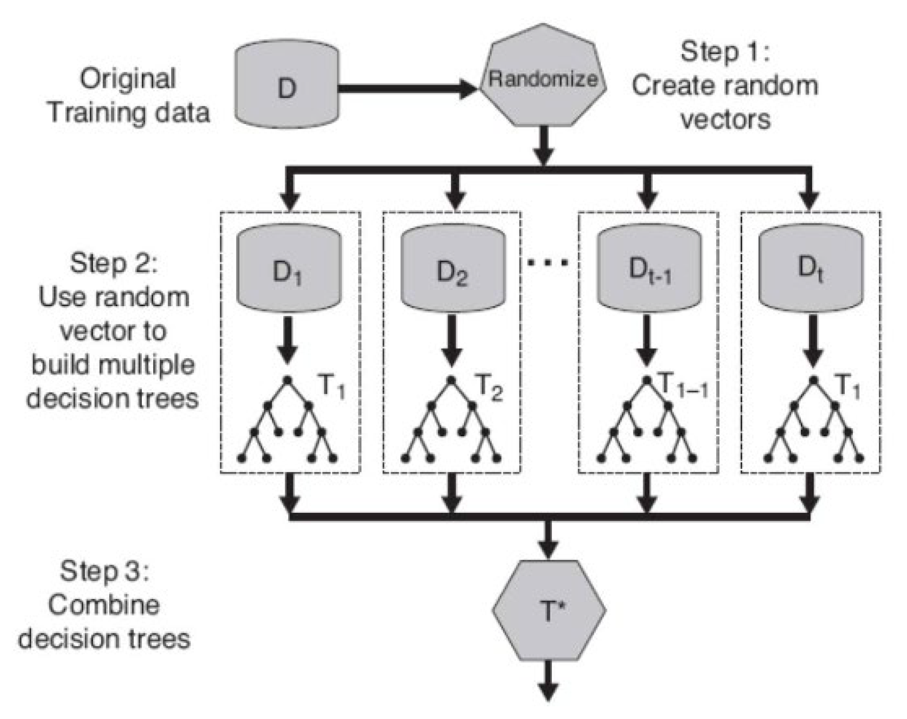
A crucial decision in step (ii) is to determine the tree hyperparameters of the RF, including the level of the depth tree and the minimum number of instances in a leaf node of the tree. Both hyperparameters of the RF are tuned somewhat through 5-fold cross-validation data using the grid search method.
C. Support Vector Classification Model
Some linear classification models, such as logistic regression (LR) or Fisher linear discriminant (FDL), are poorly defined because they have many possible lines separating the two classes as the decision boundary. Therefore, a classification model with a better definition is required to achieve the best one with satisfactory performance. An option model is a maximum margin classification that maximizes the distance between the decision boundary and nearest training instances by providing the maximum slack for classifying new cases.
The margin of an SVM classifier is the smallest distance between the decision boundary and any training instance called a support vector [64]. Figure 4 describes the relationship among the components of an SVM model, including the decision boundary (separating hyperplane), decision margin, and support vectors. A support vector is a training point that lies on the decision-margin line. The SVM concept involves finding support vectors that minimize the distance between two decision margin lines. In other words, the SVM task is the same as maximizing the vectors of x nearest to the decision boundary [65].
Figure 4 shows three types of points: well-classified points (, points lying within the margin ( ), and misclassified points ( ). All the cases can be rewritten as Equation (1) as follows:
where , are called slack variable constraints. The SVM optimization problem involves maximizing the margin and minimizing the slack variable. The optimization formulation is as follows:
subject to
and
Equation (2) is formulated using the Lagrange multiplier to obtain Equation (3), as follows:
where and . To minimize is done by set , and finally, rewrite the dual problem formulation given in Equation (4) as the following [66]:
Subject to
The C constant is the hyperparameter of the SVM model, which is the inverse of the regularization strength. C has a behavior: if the C value increases, then the model becomes overfitted. On the other hand, if the C value decreases, the model becomes underfitted.
The last part of Equation (4) can be substituted by a kernel function that acts as a nonlinear mapping from a low-dimensional feature space to a high-dimensional feature space to simplify the optimization problem. This is known as the kernel-trick method. Mathematically, the formula for a kernel function is defined as
where k is the kernel and is the feature map. The decision function of the SVM model in the feature-map space is expressed as follows:
where
An instance x is classified by involving a kernel with the following formula
with as the target class of the instance, and the bias b is calculated using
The w and b formulas above were obtained through the Karush Kuhn Tucker (KKT) conditions.
The Radial Bases Function (RBF) kernel is defined as
Equation (5) 's denominator (used only for the RBF kernel) is called the gamma value, which is the hyperparameter of the RBF kernel. The gamma value exhibits a behavior such that as it increases, the model becomes overfitted. However, as it decreases, the model becomes underfitted.
D. Performance Metrics of Classification Model
All of the performance metrics to evaluate classifier models of binary classes are calculated using the elements of a confusion matrix, such as that given in Equation (6), as follows:
where TN, FN, FP, and TP represent true negatives, false negatives, false positives, and true positives, respectively [67]. This study employs the six metrics presented in Equation (7) as follows:
Performance metrics, including accuracy, precision, recall, and F1 score, are famous metrics often used as performance measures for evaluating classifier models in binary classification with balanced classes. Two other metrics, namely Matthews Correlation Coefficient (MCC) and Area Under ROC Curve (AUC), were employed to evaluate the classifier performance more comprehensively [68].
The MCC metric is widely used to evaluate the performance of classifier models in biomedical research. Both MCC and AUC are elective metrics for reaching a consensus on the best practices for the development and validation of predictive models for personalized medicine [69]. The AUC value ranges from 0.0 to 1.0, describing the capability of the binary classifier to separate instances of the positive class (class_1) from instances of the negative class (class_0).
IV. Result and Discussion
A commensurate measure related to the numerical features of the dataset is the first issue faced in the preprocessing stage. The various measurement units were handled by transforming them into a standardized Gaussian (Z score) with a zero mean and a variance of 1. Normalized data provides an easy way to trace outlier values. An observation value is an outlier value when its absolute Z-score exceeds 3. If an instance contains an outlier value for any feature, it is dropped from the dataset. The last version of the dataset has commensurate measures, and no outliers are split into the training and testing sets.
A. Do Oversampling and Format 5 Pairs of the Training and Validation Subsets
The dataset with all predictor features was randomly split into training (80%) and testing (20%) sets. The random forest (RF) and support vector machine (SVM) models were developed by employing a training set that trained the models and five pairs of training and validation subsets for tuning hyperparameter purposes. The testing set acts as out-of-sample data for evaluating the performance of the best model, which is the one with the optimal hyperparameters. Because the dataset has an imbalanced class, the issue has to be overcome by conducting oversampling before the training set is divided randomly into five folds of cross-validation data. It is known that the target feature has a class label distribution of [class_0, class_1] = [36155, 611], which clearly shows an imbalanced distribution. The oversampling method was conducted on the class with the lower frequency (class_1) until the class_1 frequency was the same as the class_0 frequency. Figure 5 shows that both the classes had the same frequency.
By applying the oversampling method, the class_1 frequency increased from 611 to 36155, affecting the total number of instances in the oversampling training set to 72310. The application of oversampling creates a trade-off that must be paid for model training, and hyperparameter tuning consumes a longer processing time. Furthermore, the oversampling training set was divided randomly into five folds and formatted into the five training and validation subsets. The number of instances in each fold or validation subset is 14462. The training subset was used to train model candidates on a given hyperparameter pair, and the validation subset was employed to calculate the accuracy metric of the model performance. Each hyperparameter pair was used to train a model candidate in five training subsets that produced five accuracy values from the five validation subsets. The average of the five accuracy values represents the model candidate's performance on the given hyperparameter pair.
B. Tunining Hyperparameters of Random Forest Classification
In building the random forest (RF) model, this research considers two types of hyperparameters that are supposed to influence RF performance greatly. Both hyperparameters are the minimum number of instances on the tree leaf node and the depth level of the trees in the forest. The range values of the hyperparameters expected to cover the optimal one are determined first by trial and error. Finally, the minimum number of instances on the tree leaf node was set as [300, 500, 700, 1000, 1200], and the depth level of the trees was set as [7, 8, 9, 10, 12, 14]. Each combination of both values is employed to train the RF model candidate using the training subset, the union of four-folds, and the accuracy performance is calculated on the corresponding validation subset, with one remaining fold. Because there are five training subsets and five validation subsets, each pair of hyperparameters is employed five times to train the RF model candidate, and the accuracy metric of each model yielded is calculated using the corresponding validation subset. The model accuracy performance on a pair of hyperparameters was the average accuracy of the model on five validation subsets. Figure 6 shows the average accuracy metric of the 30-pair combination of hyperparameters.
The average accuracy of the RF model candidates for various pairs of hyperparameters is shown in Figure 6. The average accuracy increases consistently, which follows an increase in the depth level of the trees. Considering the increasing average accuracy pattern preceding depth levels of trees of 10, the average accuracy always increases by more than 6% if the depth level of the trees in the RF increases by two points. Nevertheless, a different pattern occurs when the depth level of the trees is more significant than 10, and the increasing average accuracy update is lower than the increasing average accuracy in the preceding depth level of the trees. There is only an increasing average accuracy of approximately 4%, where the depth level of the trees increases from 10 to 12 points. This phenomenon implicitly shows that overfitting will occur when the depth level of the trees in the RF is greater than 10. However, the hyperparameter of the minimum number of instances in the tree leaf node did not significantly affect the shifting of average accuracy values. The average accuracy of the depth levels of trees of 10 is in the range of 0.828-0.830, where the maximum average accuracy occurs on the hyperparameter pair of [500, 10], which is selected as the best one. The best hyperparameter pair was used to train the RF model using an oversampling training set. The confusion matrix of the optimal RF model was calculated for both the training and testing sets, as given in Table 3, as follows:
Table 3 presents the confusion matrices in both the RF training and testing sets with hyperparameters [500, 10]. The optimal RF incorrectly classified 9826 of 36155 instances in the negative class (class_0) on the training set and incorrectly classified 2511 of 9023 instances in class_0 on the testing set. Furthermore, the optimal RF incorrectly classified 36 of 611 instances in the positive class (class_1) in the training set and incorrectly classified 84 of 169 instances in class_1 in the testing set.
C. Tuning Hyperparameter of the Support Vector Classification Model
In developing the support vector machine (SVM) classification, the constant and gamma values are two hyperparameters tuned through cross-validation data. The range value for the optimal hyperparameter was determined carefully. First, the SVM model candidate was trained by a given constant value and various gamma values to acquire the gamma value with the highest accuracy performance and pick it up as the selected gamma value. Furthermore, the SVM model was again trained using the selected gamma and various constant values. Finally, it is obtained sets of gamma and constant values which are [0.0001, 0.0005, 0.001, 0.005, 0.01] and [100, 500, 1000, 3000, 5000, 10000]. Each combination of hyperparameters consisting of 30 pairs was used to train the SVM model candidate in the training set, which was the union of four-folds, and the accuracy performance on the associated validation set, which was one remaining fold, was calculated. The average accuracy performance for all folds and pairs of gamma and constant values is presented as a heat map in Figure 7.
Figure 7 presents the SVM model candidate's average accuracy values in the gamma coordinates and constant hyperparameters' coordinates. They appear randomly distributed and compete tightly with each other. The best accuracy occurred in the pair value of [0.001, 500] for the gamma and constant values, respectively. The hyperparameter pair associated with the SVM model had an average accuracy of 0.668. Furthermore, the yielded hyperparameter pair [0.001, 500] was employed to train the SVM model candidate using the oversampling training data, and the confusion matrix in both the training and testing sets is given in Table 4.
Table 4 shows the SVM confusion matrix in which the model incorrectly classified 13342 of 36155 instances in the training set's negative class (class_0) and incorrectly classified 3562 of 9023 instances in the negative class of the testing set. Subsequently, the model incorrectly classified 192 of 611 instances in the training set's positive class (class_1) and classified 65 of 169 instances in class_1 of the testing set. The SVM model better classified the class_1 instance in the testing set than the RF model. Nevertheless, the RF performed better than the SVM in the training part. The SVM model average accuracy presented in the heat map had a random distribution that implies no occurrence of the overfitting problem. In addition, it must be highlighted that training the SVM in 5-fold validation data consumed longer than the RF training.
D. The Comparison of Models Performance and the Important Features
Performance metrics, including accuracy, precision, recall, F1 score, MCC, and AUC, were calculated in both the training and testing sets to compare the RF and SVM models comprehensively. In addition, the optimal hyperparameters were employed to train both models using the original training set (not the oversampling training set) as a benchmark. Table 5 presents the performance of the benchmark and best models in the training and testing sets. Table 5 has two primary columns: the first consists of columns presenting the RF performance, and the second consists of columns explaining the SVM performance. Each central column contains four columns, where the first and second columns show the benchmark model performance, and the two remaining columns present the best model performance.
In the performance evaluation of the RF model in the training set, the RF benchmark model performed 98% in four metrics: accuracy, precision, recall, and F1 score. In comparison, it performed 15% and 51.2% for the MCC and AUC metrics, respectively. On the other hand, the best RF model has a lower performance than the RF benchmark in the three metrics. Still, it performs with the same precision as the RF benchmark and performs better with gaps in both metrics of 4% and 32.3% for the MCC and AUC, respectively.
Evaluating the RF model in the testing set, the RF benchmark performs better than the best RF in the three metrics, including the accuracy, recall, and F1 score, with gaps of 26.4%, 26%, and 15%, respectively. However, the best RF performs better than the RF benchmark for precision, MCC, and AUC, with gaps of 1%, 6.7%, and 11.2%, respectively. The RF benchmark performs 0% on the MCC and 50% on the AUC, which is the same as the probability of a toss-balanced coin, or the RF benchmark has no performance. Although the best RF model performed lower than the RF benchmark in the three famous metrics, it performed significantly better than the MCC and AUC metrics, which were 6.7% and 61.2%, respectively. Conducting oversampling increased the MCC and AUC values by 6.7 and 11.2%, respectively.
By evaluating the SVM models in the training set, the SVM benchmark model performs with the same precision of 97% as the best SVM model, and both models have performance gaps of 35.1%, 35%, and 21% for the metrics of accuracy, recall, and F1 score, respectively. In addition, the best SVM performs better than the benchmark, with gaps of 8.5% and 15.8% for the MCC and AUC metrics, respectively. In evaluating the SVM models in the testing set, the SVM benchmark model performed better than the best SVM for accuracy, recall, and F1 score metrics with gaps of 37.7%, 37%, and 24%, respectively. In contrast, the best SVM performed better than the benchmark model for the precision, MCC, and AUC metrics with gaps of 1%, 5.6%, and 11.1%, respectively.
The performance of the SVM benchmark on the test set was almost identical to that of the RF benchmark. Both benchmark models do nothing, as indicated by the MCC metric of 0 and the AUC metric of 0.5. This explains why neither benchmark model can correctly predict the labels of unknown positive class instances in the test set. Extensive efforts have been made to tune the hyperparameters to produce a well-performing classification model but ended up in vain. The best RF model performed similarly to the best SVM model for training and test sets. In the training set, the best RF performed slightly better than the best SVM, with gaps of 10%, 1%, 10%, 7%, 10.5%, and 17.7% for the metrics accuracy, precision, recall, F1 score, MCC, and AUC, respectively. In the test set, the best RF performs slightly better than the best SVM for the metrics accuracy, recall, F1 score, MCC, and AUC with gaps of 11.3%, 11%, 8%, 1.1%, and 0.1%, respectively. Except for the precision metric, the best SVM is better than the best RF by a margin of 1%.
The results confirmed that the oversampling method performed on class imbalance to train machine learning models can improve the model performance. This is similar to the work done by [20], [29], and [30]. The MCC or AUC metrics clearly explain performance improvements. The MCC value increased by 6.7% and 5.6% for the best RF and SVM models, respectively, whereas the AUC value of both models was approximately 11%. Although the best RF model performs slightly better than the best SVM model, searching for optimal hyperparameters in the RF model must be careful. Otherwise, there is a potential for overfitting problems [55]. Additionally, other findings indicated by the benchmark model should receive significant attention. The benchmark model has a high performance of approximately 98% on both the training and test sets in four performance metrics: accuracy, precision, recall, and F1 score. However, both benchmark models performed nothing in the test set, as indicated by an MCC value of 0 and an AUC value of 0.5, where their performance was only equal to the probability of a balanced coin toss [25]. The event implicitly recommends that using four famous metrics to evaluate the model performance of imbalanced binary classes is foolish.
In machine learning modeling, evaluating the model's performance on the test set is more important because it depicts its ability to classify the out-of-sample data. This study presents a performance evaluation of the training and test sets to implicitly show that the goodness-of-fit model obtained based on the training set can lead to biased inferences. The model had a lower performance on the test set, but the pattern of performance metrics was similar when the model did not suffer from overfitting problems [52]. Obtaining an optimal RF model is constrained by the difficulty of determining the hyperparameter domain that includes optimal values. However, running the RF model on cross-validation data requires less time. On the other hand, the hyperparameter domain of an SVM model can be determined easily, but running the SVM model on cross-validation data is an arduous task that takes a long time.
Another advantage of building an RF model is that it is an important feature that needs to be explored. The degree of importance of each feature can be used to determine the dominant features or for dimension reduction [10]. Developing a model that involves a few predictor features is preferable because the system mechanism underlying the model can be explained and interpreted well [42]. Figure 8 presents the degree of essential features produced by the best RF model.
The bar chart in Figure 8 presents the ranking of important features in increasing order. The numerical features appear to dominate the degree of higher importance, acting as the splitting feature in developing the RF model. The first five important features are CBC_Platelet, AGE, K, GOT, and LOS, with a degree of importance of approximately 10%, 9$, 8%, 8%, and 8%, respectively. This means that the five features have a role of approximately 43% in developing the RF model. The next group has four features, each with a degree of importance of roughly 6%, followed by Na and GPT features with a degree of importance of approximately 5%. There were five features with a degree of importance of roughly 3%. The importance of the first 16 critical features is approximately 92%. From the viewpoint of dimension reduction, 16 features could explain the total variance in the dataset by approximately 92%. It is supposed to be noted that all of the 12 numerical features are included as important features.
V. Conclusion
Applying the oversampling method significantly increased the number of instances for hyperparameter tuning, where the number of cases in the training set increased almost twice. This consumes a lot of time, especially when running SVM models on cross-validation data for hyperparameter tuning. The optimal hyperparameter pair obtained by the RF model is [500,10]; that is, the minimum number of instances in the tree's leaf nodes is 500, and the tree depth level in the RF is 10. Meanwhile, the optimal hyperparameter pair from the SVM model is [1000, 0.05], namely, the hyperparameter constant value of 1000 and the hyperparameter gamma value of 0.05.
The RF and SVM benchmark models have high-performance values of 98% for accuracy, precision, recall, and Fi score metrics. Still, both benchmark models do nothing in MCC and AUC metrics, with 0 and 50% values, respectively. In contrast, the best RF and SVM models performed similarly for the six metrics. The two best models had lower performance than the two benchmark models on accuracy, precision, recall, and F1 score. Nevertheless, the best models performed better than the benchmark models on the MCC and AUC metrics. The best RF performance experienced an increase in the MCC value of 6.7% and an AUC value of 11.2%, whereas the best SVM performance experienced an increase in the MCC value of 5.6% and an AUC value of 11.1%. The best RF model performed better than the best SVM, with slightly different MCC and AUC metrics performance. In addition, the RF model produces important features that can be potential inputs for building other machine-learning models. In future research, building an RF model using the original feature scale and MCC or AUC as selection criteria to obtain optimal hyperparameters is expected to improve the model performance significantly.
Author Contributions
Conceptualization, Samingun Handoyo and Ying-Ping Chen; Data curation, Ratno Bagys Wibowo and Agus Widodo; Formal analysis, Ratno Bagys Wibowo; Investigation, Ying-Ping Chen and Agus Widodo; Methodology, Samingun Handoyo; Resources, Ratno Bagys Wibowo; Software, Samingun Handoyo and Agus Widodo; Validation, Ying-Ping Chen; Writing – original draft, Samingun Handoyo; Writing – review & editing, Ying-Ping Chen.
Conflicts of Interest
The authors declare no conflict of interest related to this research project.
References
- A. W. Widodo, S. Handoyo, G. Irianto, N. W. Hidajati, D. S. Susanti, and I. N. Purwanto, “Finding the Best Performance of Bayesian and Naïve Bayes Models in Fraudulent Firms Classification through Varying Threshold,” International Journal of Emerging Technology and Advanced Engineering, vol. 12, no. 12, pp. 94–106, Dec. 2022. [CrossRef]
- S. Syahrial, R. Ilham, Z. F. Asikin, and St. S. I. Nurdin, “Stunting Classification in Children’s Measurement Data Using Machine Learning Models,” Journal La Multiapp, vol. 3, no. 2, 2022. [CrossRef]
- W. Cnota et al., “The Killer Placenta” — a threat to the lives of young women giving Birth by cesarean section,” Ginekol Pol, vol. 93, no. 4, 2022. [CrossRef]
- T. Liu, W. Fan, and C. Wu, “A hybrid machine learning approach to cerebral stroke prediction based on the imbalanced medical dataset,” Artif Intell Med, vol. 101, 2019. [CrossRef]
- I. D. Mienye and Y. Sun, “Performance analysis of cost-sensitive learning methods with application to imbalanced medical data,” Inform Med Unlocked, vol. 25, 2021. [CrossRef]
- A. V. Barmak, Y. V. Krak, E. A. Manziuk, and V. S. Kasianiuk, “Information technologyof separating hyperplanes synthesisfor linear classifiers,” Journal of Automation and Information Sciences, vol. 51, no. 5, 2019. [CrossRef]
- Priyanka and D. Kumar, “Decision tree classifier: A detailed survey,” International Journal of Information and Decision Sciences, vol. 12, no. 3, 2020. [CrossRef]
- T. Lan, H. Hu, C. Jiang, G. Yang, and Z. Zhao, “A comparative study of decision tree, random forest, and convolutional neural network for spread-F identification,” Advances in Space Research, vol. 65, no. 8, 2020. [CrossRef]
- J. L. Speiser, M. E. Miller, J. Tooze, and E. Ip, “A comparison of random forest variable selection methods for classification prediction modeling,” Expert Systems with Applications, vol. 134. 2019. [CrossRef]
- M. Z. Alam, M. S. Rahman, and M. S. Rahman, “A Random Forest based predictor for medical data classification using feature ranking,” Inform Med Unlocked, vol. 15, 2019. [CrossRef]
- S. El-Sappagh, F. Ali, T. Abuhmed, J. Singh, and J. M. Alonso, “Automatic detection of Alzheimer’s disease progression: An efficient information fusion approach with heterogeneous ensemble classifiers,” Neurocomputing, vol. 512, 2022. [CrossRef]
- J. Cervantes, F. Garcia-Lamont, L. Rodríguez-Mazahua, and A. Lopez, “A comprehensive survey on support vector machine classification: Applications, challenges and trends,” Neurocomputing, vol. 408, 2020. [CrossRef]
- W. Pannakkong, K. Thiwa-Anont, K. Singthong, P. Parthanadee, and J. Buddhakulsomsiri, “Hyperparameter Tuning of Machine Learning Algorithms Using Response Surface Methodology: A Case Study of ANN, SVM, and DBN,” Math Probl Eng, vol. 2022, 2022. [CrossRef]
- X. Ding, J. Liu, F. Yang, and J. Cao, “Random radial basis function kernel-based support vector machine,” J Franklin Inst, vol. 358, no. 18, 2021. [CrossRef]
- A. Kumar, N. Sinha, and A. Bhardwaj, “A novel fitness function in genetic programming for medical data classification,” J Biomed Inform, vol. 112, 2020. [CrossRef]
- J. Bektaş, “EKSL: An effective novel dynamic ensemble model for unbalanced datasets based on LR and SVM hyperplane-distances,” Inf Sci (N Y), vol. 597, 2022. [CrossRef]
- M. A. Ganaie and M. Tanveer, “KNN weighted reduced universum twin SVM for class imbalance learning,” Knowl Based Syst, vol. 245, 2022. [CrossRef]
- D. Chicco and G. Jurman, “The advantages of the Matthews correlation coefficient (MCC) over F1 score and accuracy in binary classification evaluation,” BMC Genomics, vol. 21, no. 1, 2020. [CrossRef]
- G. Canbek, T. Taskaya Temizel, and S. Sagiroglu, “BenchMetrics: a systematic benchmarking method for binary classification performance metrics,” Neural Comput Appl, vol. 33, no. 21, 2021. [CrossRef]
- G. Kovács, “An empirical comparison and evaluation of minority oversampling techniques on a large number of imbalanced datasets,” Applied Soft Computing Journal, vol. 83, 2019. [CrossRef]
- Z. Xu, D. Shen, T. Nie, Y. Kou, N. Yin, and X. Han, “A cluster-based oversampling algorithm combining SMOTE and k-means for imbalanced medical data,” Inf Sci (N Y), vol. 572, 2021. [CrossRef]
- D. Passos and P. Mishra, “A tutorial on automatic hyperparameter tuning of deep spectral modelling for regression and classification tasks,” Chemometrics and Intelligent Laboratory Systems, vol. 223. 2022. [CrossRef]
- S. Nematzadeh, F. Kiani, M. Torkamanian-Afshar, and N. Aydin, “Tuning hyperparameters of machine learning algorithms and deep neural networks using metaheuristics: A bioinformatics study on biomedical and biological cases,” Comput Biol Chem, vol. 97, 2022. [CrossRef]
- R. Yacouby and D. Axman, “Probabilistic Extension of Precision, Recall, and F1 Score for More Thorough Evaluation of Classification Models,” 2020. [CrossRef]
- D. Chicco and G. Jurman, “The Matthews correlation coefficient (MCC) should replace the ROC AUC as the standard metric for assessing binary classification,” BioData Min, vol. 16, no. 1, 2023. [CrossRef]
- S. Handoyo, Y. P. Chen, G. Irianto, and A. Widodo, “The varying threshold values of logistic regression and linear discriminant for classifying fraudulent firm,” Mathematics and Statistics, vol. 9, no. 2, 2021. [CrossRef]
- H. Zhou, K. M. Yu, Y. C. Chen, and H. P. Hsu, “A Hybrid Feature Selection Method RFSTL for Manufacturing Quality Prediction Based on a High Dimensional Imbalanced Dataset,” IEEE Access, vol. 9, 2021. [CrossRef]
- A. S. Sumant and D. V. Patil, “Parallel Ensemble Feature Subset Selection based Deep Learning Approach for Imbalanced High Dimensional Cancer Datasets,” Indian Journal of Computer Science and Engineering, vol. 13, no. 6, 2022. [CrossRef]
- T. Wongvorachan, S. He, and O. Bulut, “A Comparison of Undersampling, Oversampling, and SMOTE Methods for Dealing with Imbalanced Classification in Educational Data Mining,” Information (Switzerland), vol. 14, no. 1, 2023. [CrossRef]
- A. S. Desuky and S. Hussain, “An Improved Hybrid Approach for Handling Class Imbalance Problem,” Arab J Sci Eng, vol. 46, no. 4, 2021. [CrossRef]
- W. Lu, Z. Li, and J. Chu, “Adaptive Ensemble Undersampling-Boost: A novel learning framework for imbalanced data,” Journal of Systems and Software, vol. 132, 2017. [CrossRef]
- P. Roy and C. Chowdhury, “A Survey of Machine Learning Techniques for Indoor Localization and Navigation Systems,” Journal of Intelligent and Robotic Systems: Theory and Applications, vol. 101, no. 3, 2021. [CrossRef]
- Marji, S. Handoyo, I. N. Purwanto, and M. Y. Anizar, “The effect of attribute diversity in the covariance matrix on the magnitude of the radius parameter in fuzzy subtractive clustering,” J Theor Appl Inf Technol, vol. 96, no. 12, 2018.
- I. N. Purwanto, A. Widodo, and S. Handoyo, “System for selection starting lineup of a football players by using analytical hierarchy process (AHP),” J Theor Appl Inf Technol, vol. 96, no. 1, 2018.
- S. Handoyo, Marji, I. N. Purwanto, and F. Jie, “The fuzzy inference system with rule bases generated by using the fuzzy C-means to predict regional minimum wage in Indonesia,” International Journal of Operations and Quantitative Management, vol. 24, no. 4, 2018.
- L. Liu, N. Jia, L. Lin, and Z. He, “A Cohesion-Based Heuristic Feature Selection for Short-Term Traffic Forecasting,” IEEE Access, vol. 7, 2019. [CrossRef]
- W. H. Nugroho, S. Handoyo, and Y. J. Akri, “An influence of measurement scale of predictor variable on logistic regression modeling and learning vector quntization modeling for object classification,” International Journal of Electrical and Computer Engineering, vol. 8, no. 1, 2018. [CrossRef]
- Marji and S. Handoyo, “PERFORMANCE OF RIDGE LOGISTIC REGRESSION AND DECISION TREE IN THE BINARY CLASSIFICATION,” J Theor Appl Inf Technol, vol. 100, no. 15, 2022.
- M. Koklu and I. A. Ozkan, “Multiclass classification of dry beans using computer vision and machine learning techniques,” Comput Electron Agric, vol. 174, 2020. [CrossRef]
- S. Handoyo, N. Pradianti, W. H. Nugroho, and Y. J. Akri, “A Heuristic Feature Selection in Logistic Regression Modeling with Newton Raphson and Gradient Descent Algorithm,” International Journal of Advanced Computer Science and Applications, vol. 13, no. 3, 2022. [CrossRef]
- N. Han et al., “Transferable Linear Discriminant Analysis,” IEEE Trans Neural Netw Learn Syst, vol. 31, no. 12, 2020. [CrossRef]
- Y. T. Mursityo, I. Rupiwardani, W. H. N. Putra, D. S. Susanti, T. Handayani, and S. Handoyo, “Relevant Features Independence of Heuristic Selection and Important Features of Decision Tree in the Medical Data Classification,” Journal of Advances in Information Technology, vol. 15, no. 5, pp. 591–601, 2024. [CrossRef]
- P. H. Huynh and V. H. Nguyen, “A Novel Ensemble of Support Vector Machines for Improving Medical Data Classification,” Engineering Innovations, vol. 4, 2023. [CrossRef]
- M. M. Chen and M. C. Chen, “Modeling road accident severity with comparisons of logistic regression, decision tree, and random forest,” Information (Switzerland), vol. 11, no. 5, 2020. [CrossRef]
- A. Subudhi, M. Dash, and S. Sabut, “Automated segmentation and classification of brain stroke using expectation-maximization and random forest classifier,” Biocybern Biomed Eng, vol. 40, no. 1, 2020. [CrossRef]
- A. Al-Hashedi et al., “Ensemble Classifiers for Arabic Sentiment Analysis of Social Network (Twitter Data) towards COVID-19-Related Conspiracy Theories,” Applied Computational Intelligence and Soft Computing, vol. 2022, 2022. [CrossRef]
- M. Aslani and S. Seipel, “Efficient and decision boundary aware instance selection for support vector machines,” Inf Sci (N Y), vol. 577, 2021. [CrossRef]
- A. Widodo and S. Handoyo, “The classification performance using logistic regression and support vector machine (SVM),” J Theor Appl Inf Technol, vol. 95, no. 19, 2017.
- T. Y. Wen and S. A. Mohd Aris, “Hybrid Approach of EEG Stress Level Classification Using K-Means Clustering and Support Vector Machine,” IEEE Access, vol. 10, 2022. [CrossRef]
- G. Bologna and Y. Hayashi, “A Comparison Study on Rule Extraction from Neural Network Ensembles, Boosted Shallow Trees, and SVMs,” Applied Computational Intelligence and Soft Computing, vol. 2018, 2018. [CrossRef]
- S. K. Saddam Hussain, E. Sai Charan Reddy, K. Gangadhar Akshay, and T. Akanksha, “Fraud Detection in Credit Card Transactions Using SVM and Random Forest Algorithms,” in Proceedings of the 5th International Conference on I-SMAC (IoT in Social, Mobile, Analytics and Cloud), I-SMAC 2021, 2021. [CrossRef]
- A. Sabat-Tomala, E. Raczko, and B. Zagajewski, “Comparison of support vector machine and random forest algorithms for invasive and expansive species classification using airborne hyperspectral data,” Remote Sens (Basel), vol. 12, no. 3, 2020. [CrossRef]
- M. Hesami and A. M. P. Jones, “Modeling and optimizing callus growth and development in Cannabis sativa using random forest and support vector machine in combination with a genetic algorithm,” Appl Microbiol Biotechnol, vol. 105, no. 12, 2021. [CrossRef]
- C. G. Siji George and B. Sumathi, “Grid search tuning of hyperparameters in random forest classifier for customer feedback sentiment prediction,” International Journal of Advanced Computer Science and Applications, vol. 11, no. 9, 2020. [CrossRef]
- D. Sun, J. Xu, H. Wen, and D. Wang, “Assessment of landslide susceptibility mapping based on Bayesian hyperparameter optimization: A comparison between logistic regression and random forest,” Eng Geol, vol. 281, 2021. [CrossRef]
- M. Daviran, A. Maghsoudi, R. Ghezelbash, and B. Pradhan, “A new strategy for spatial predictive mapping of mineral prospectivity: Automated hyperparameter tuning of random forest approach,” Comput Geosci, vol. 148, 2021. [CrossRef]
- I. S. Al-Mejibli, J. K. Alwan, and D. H. Abd, “The effect of gamma value on support vector machine performance with different kernels,” International Journal of Electrical and Computer Engineering, vol. 10, no. 5, 2020. [CrossRef]
- J. Wainer and P. Fonseca, “How to tune the RBF SVM hyperparameters? An empirical evaluation of 18 search algorithms,” Artif Intell Rev, vol. 54, no. 6, 2021. [CrossRef]
- W. H. Nugroho, S. Handoyo, H. C. Hsieh, Y. J. Akri, Zuraidah, and D. DwinitaAdelia, “Modeling Multioutput Response Uses Ridge Regression and MLP Neural Network with Tuning Hyperparameter through Cross Validation,” International Journal of Advanced Computer Science and Applications, vol. 13, no. 9, 2022. [CrossRef]
- T. Yan, S. L. Shen, A. Zhou, and X. Chen, “Prediction of geological characteristics from shield operational parameters by integrating grid search and K-fold cross validation into stacking classification algorithm,” Journal of Rock Mechanics and Geotechnical Engineering, vol. 14, no. 4, 2022. [CrossRef]
- G. N. Ahmad, H. Fatima, Shafiullah, A. Salah Saidi, and Imdadullah, “Efficient Medical Diagnosis of Human Heart Diseases Using Machine Learning Techniques with and Without GridSearchCV,” IEEE Access, vol. 10, 2022. [CrossRef]
- Z. Chai and C. Zhao, “Enhanced random forest with concurrent analysis of static and dynamic nodes for industrial fault classification,” IEEE Trans Industr Inform, vol. 16, no. 1, 2020. [CrossRef]
- L. Gigović, H. R. Pourghasemi, S. Drobnjak, and S. Bai, “Testing a new ensemble model based on SVM and random forest in forest fire susceptibility assessment and its mapping in Serbia’s Tara National Park,” Forests, vol. 10, no. 5, 2019. [CrossRef]
- A. Murugan, S. A. H. Nair, and K. P. S. Kumar, “Detection of Skin Cancer Using SVM, Random Forest and kNN Classifiers,” J Med Syst, vol. 43, no. 8, 2019. [CrossRef]
- Y. Zhang, D. Xiao, and Y. Liu, “Automatic Identification Algorithm of the Rice Tiller Period Based on PCA and SVM,” IEEE Access, vol. 9, 2021. [CrossRef]
- D. D. Shankar and A. S. Azhakath, “Minor blind feature based Steganalysis for calibrated JPEG images with cross validation and classification using SVM and SVM-PSO,” Multimed Tools Appl, 2020. [CrossRef]
- A. W. Widodo, S. Handoyo, I. Rupiwardani, Y. T. Mursityo, I. N. Purwanto, and H. Kusdarwati, “The Performance Comparison between C4.5 Tree and One-Dimensional Convolutional Neural Networks (CNN1D) with Tuning Hyperparameters for the Classification of Imbalanced Medical Data,” International Journal of Intelligent Engineering and Systems, vol. 16, no. 5, pp. 748–759, 2023. [CrossRef]
- D. Chicco and G. Jurman, “A statistical comparison between Matthews correlation coefficient (MCC), prevalence threshold, and Fowlkes–Mallows index,” J Biomed Inform, vol. 144, 2023. [CrossRef]
- S. Boughorbel, F. Jarray, and M. El-Anbari, “Optimal classifier for imbalanced data using Matthews Correlation Coefficient metric,” PLoS One, vol. 12, no. 6, 2017. [CrossRef]
Figure 1.
The stages of the developing SVM classification model.
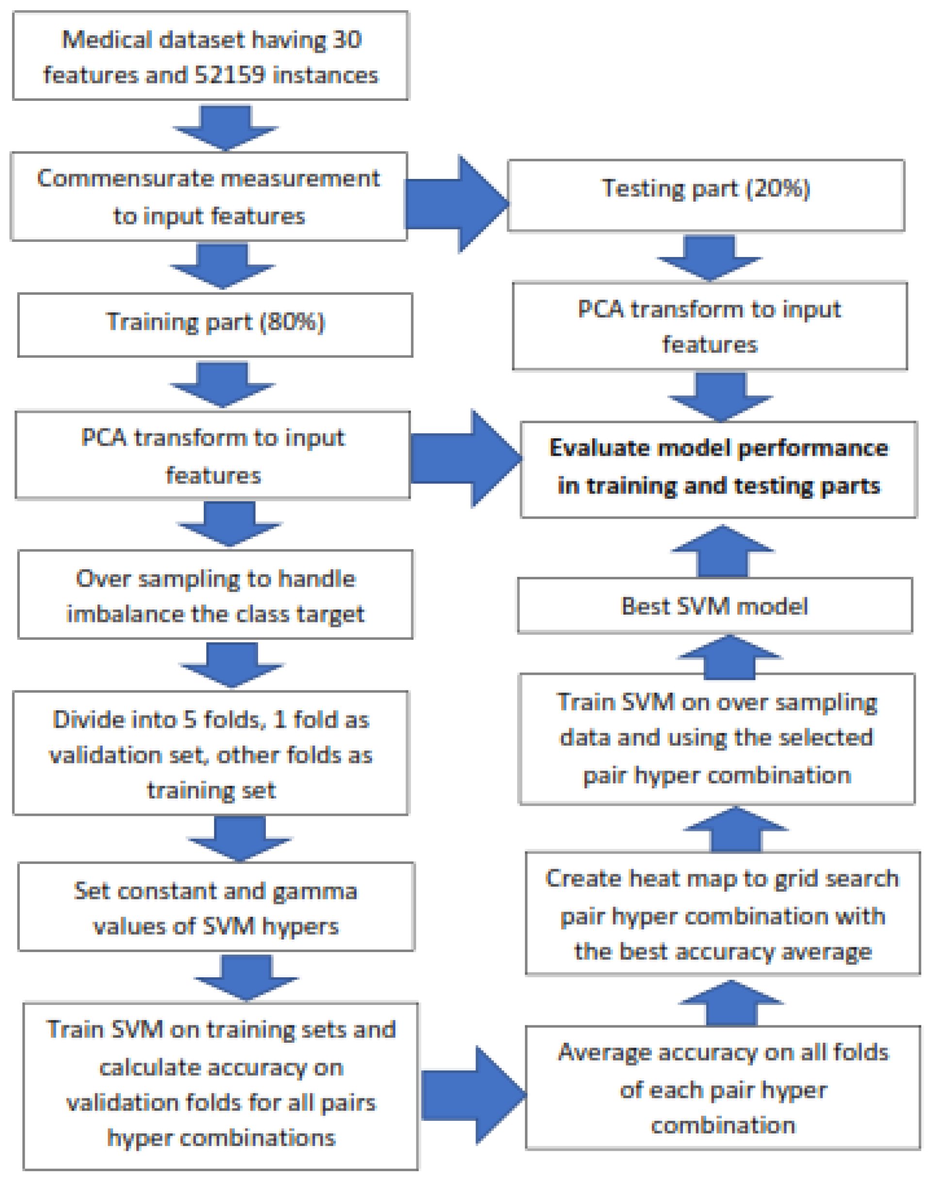
Figure 2.
Format the training set into k folds cross-validation data.
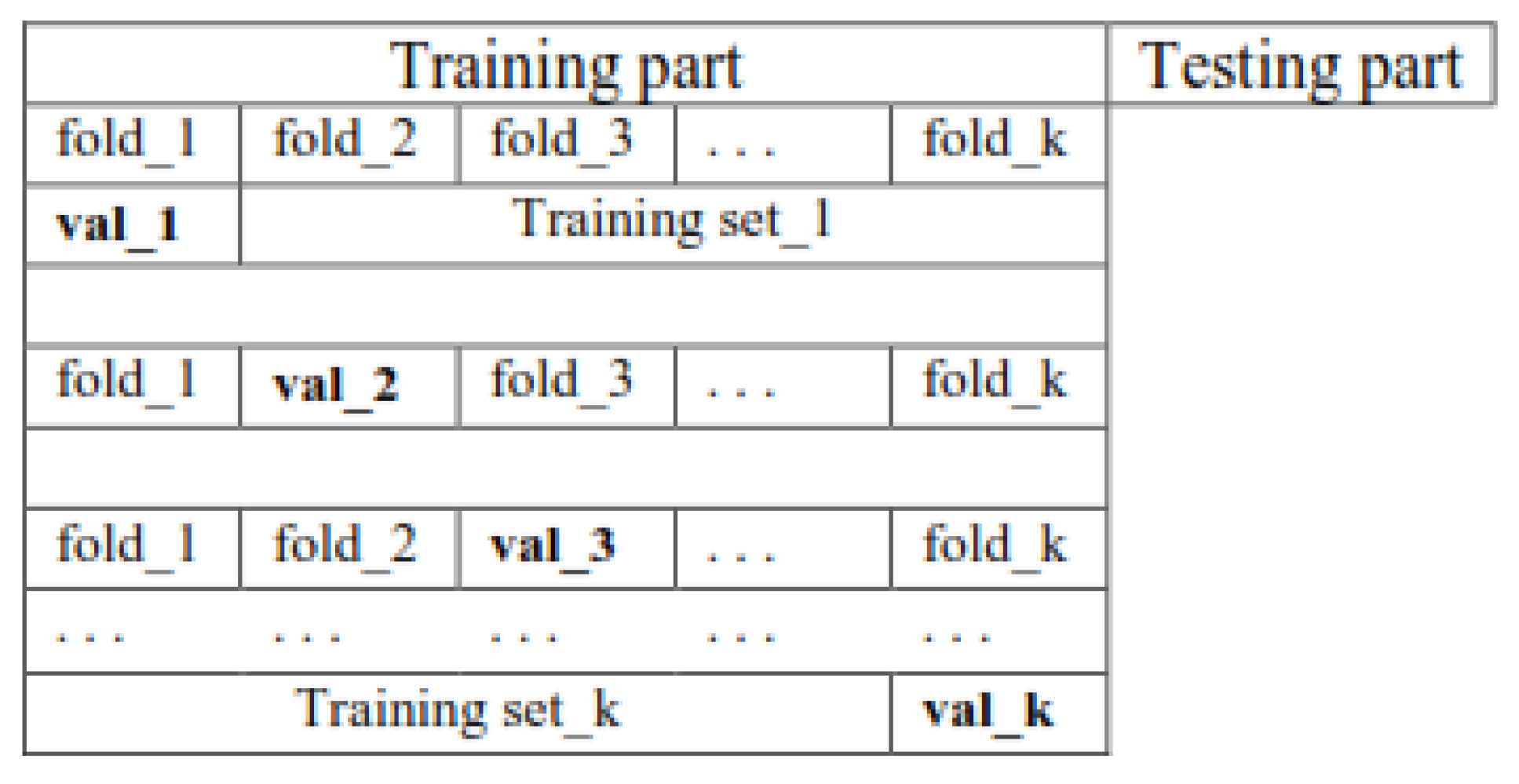
Figure 4.
The decision boundary and support vectors of an SVM model.
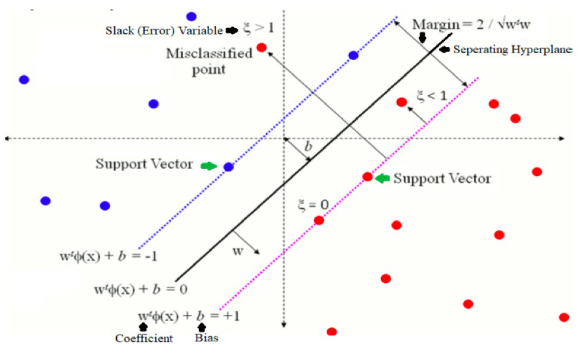
Figure 5.
Distribution of the target feature class after the conducted oversampling.
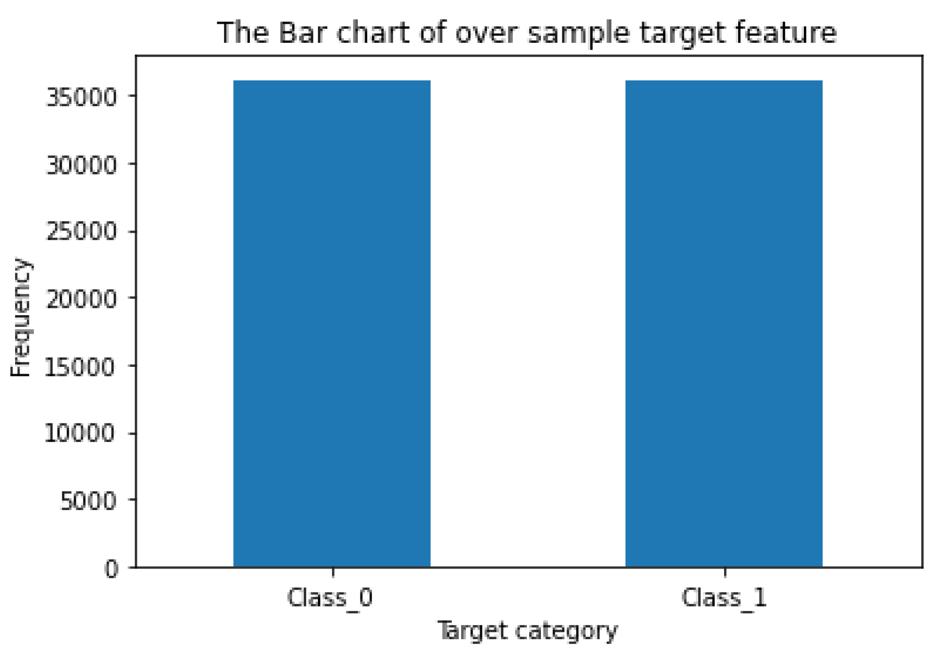
Figure 6.
The average accuracy performance of the RF in 5 validation data presented in a heat map.
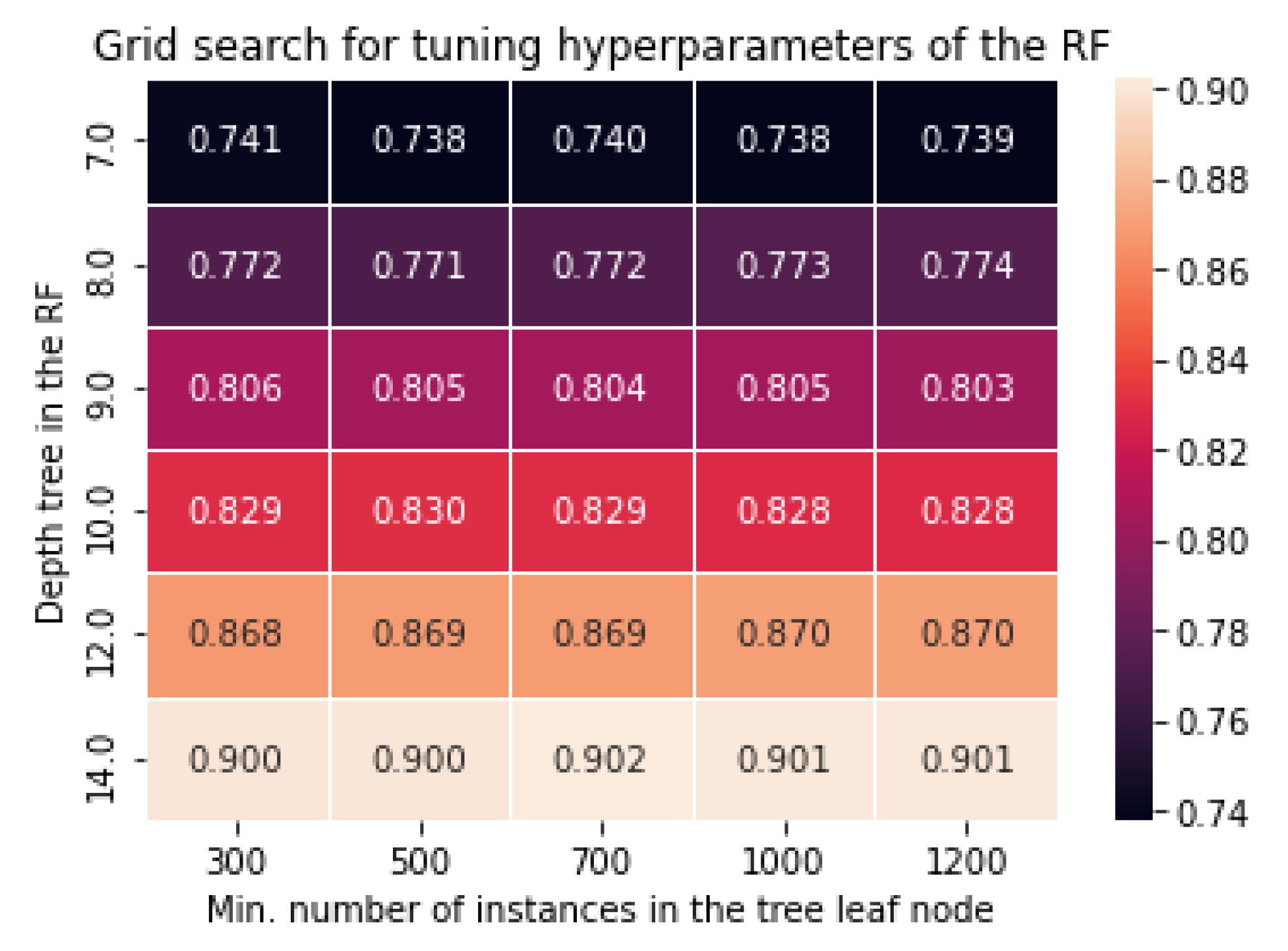
Figure 7.
The average accuracy performance of the SVM classification in 5 validation data presented in a heat map.
Figure 7.
The average accuracy performance of the SVM classification in 5 validation data presented in a heat map.
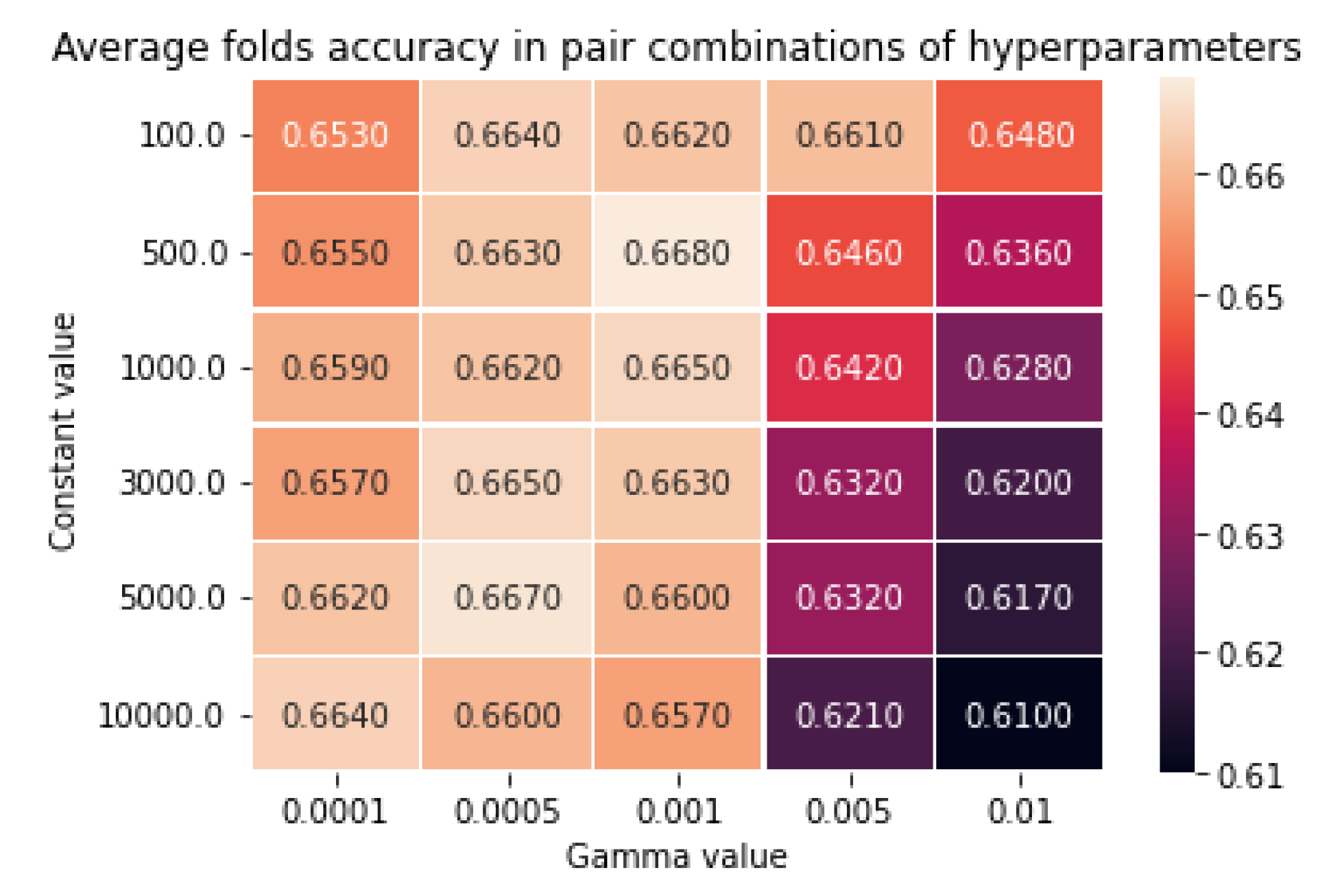
Figure 8.
The important feature is the degree of the optimal RF model.
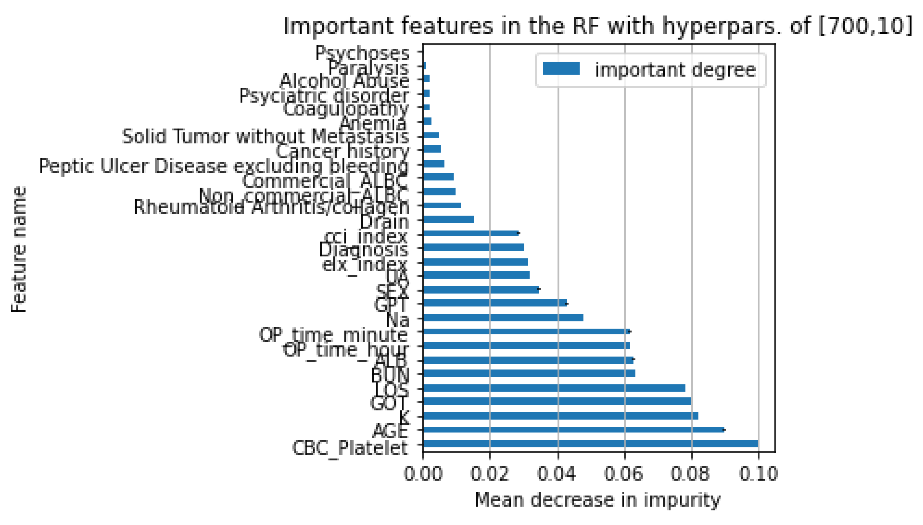

Table 1.
List of categorical features and their label distribution.
| Feature Name | Distribution Label | Labels number | Feature Name | Distribution Label | Labels number |
|---|---|---|---|---|---|
| Outcome | [51280, 879] | 2 | Commercial_ALBC | [47355, 4804] | 2 |
| Psychoses | [51999, 160] | 2 | Drain | [38550, 13609] | 2 |
| Alcohol Abuse | [51541, 618] | 2 | Paralysis | [52025, 134] | 2 |
| Coagulopathy | [51802, 357] | 2 | SEX | [34786, 17279] | 2 |
| Solid Tumor without Metastasis | [50089, 2070] | 2 | Non_commercial_ALBC | [30418, 21741] | 2 |
| Peptic Ulcer Disease, excluding bleeding | [49244, 2915] | 2 | Anemia | [51510, 629, 20] | 3 |
| Rheumatoid Arthritis/collagen | [49890, 2269] | 2 | Psychiatric disorder | [51114, 986, 59] | 3 |
| Cancer history | [50001, 1964, 193, 1] | 4 | |||
| Diagnosis | [40786, 7023, 2038, 1310, 906, 96] | 6 | |||
| elx_index | [29700, 9366, 6165, 3474, 1768, 898, 464, 188, 74, 32, 18, 9, 2, 1] | 14 | |||
| cci_index | [35002, 8003, 4343, 2301, 1172, 656, 289, 131, 117, 84, 29, 13, 12, 4, 2, 1] | 16 | |||
Table 2.
list of numerical features and their simple statistics.
| Feature name | Min. | Max. | Var. |
|---|---|---|---|
| CBC_Platelet | 16.1 | 992 | 1509.13 |
| AGE | 12 | 99 | 148.93 |
| LOS | 1 | 72 | 8.35 |
| OP_time_minute | 2 | 1539 | 1030.98 |
| OP_time_hour | 0.03 | 25.65 | 0.29 |
| BUN | 1.8 | 140.67 | 25.76 |
| GOT | 4 | 15643 | 4824.68 |
| GPT | 2 | 506 | 171.28 |
| ALB | 2 | 7.01 | 0.17 |
| Na | 22.1 | 169.32 | 3.07 |
| K | 2.3 | 8.13 | 0.17 |
| UA | 1.1 | 18.74 | 0.8 |
Table 3.
The confusion matrix of the optimal RF model.
| Actual value | Prediction training | Prediction testing | ||
| Class_0 | Class_1 | Class_0 | Class_1 | |
| Class_0 | 26329 | 9826 | 6512 | 2511 |
| Class_1 | 36 | 575 | 84 | 85 |
Table 4.
The confusion matrix of the optimal SVM with the RBF kernel.
| Actual value | Prediction training | Prediction testing | ||
| Class_0 | Class_1 | Class_0 | Class_1 | |
| Class_0 | 22813 | 13342 | 5461 | 3562 |
| Class_1 | 192 | 419 | 65 | 104 |
Table 5.
The performance comparison between the optimal rf and the optimal SVM.
| Performance measures | Random Forest (RF) | Support Vector Machine (SVM) | ||||||
|---|---|---|---|---|---|---|---|---|
| Benchmark | Best model | Benchmark | Best model | |||||
| Training | Testing | Training | Testing | Training | Testing | Training | Testing | |
| Accuracy | 0.984 | 0.982 | 0.732 | 0.718 | 0.983 | 0.982 | 0.632 | 0.605 |
| Precision | 0.980 | 0.960 | 0.980 | 0.970 | 0.970 | 0.970 | 0.970 | 0.980 |
| Recall | 0.980 | 0.980 | 0.730 | 0.720 | 0.980 | 0.980 | 0.630 | 0.610 |
| F1-score | 0.980 | 0.970 | 0.830 | 0.820 | 0.970 | 0.980 | 0.760 | 0.740 |
| MCC | 0.150 | 0.000 | 0.190 | 0.067 | 0.000 | 0.000 | 0.085 | 0.056 |
| AUC | 0.512 | 0.500 | 0.835 | 0.612 | 0.500 | 0.500 | 0.658 | 0.611 |
About the Authors
 |
Samingun Handoyo received a B.Sc. in Statistics and an M.Sc. in Computer Science from Brawijaya University and Gadjah Mada University, Indonesia. He is an Associate Professor in Science Data at Brawijaya University and a PhD candidate in Electrical Engineering and Computer Science -IGP from National Yang-Ming Chiao Tung University, Taiwan. His research interests include Machine Learning, Statistical Learning, Predictive Modeling, Fuzzy Systems, and Time Series forecasting. He has written two textbooks, The Fuzzy System Implementation with R and The Linear Time Series Analysis Application with R. |
 |
Ying-Ping Chen received the B.S. and M.S. degrees in computer science and information engineering from National Taiwan University, Taiwan, in 1995 and 1997, respectively, and the Ph.D. degree in 2004 from the Department of Computer Science, University of Illinois at Urbana-Champaign, Illinois, USA. He is currently a full professor in the Department of Computer Science at National Yang-Ming Chiao Tung University, Taiwan. His research interests include understanding intelligence via computational mechanisms and from computational perspectives, working principles, and dimensional/facet-wise models in genetic and evolutionary computation. |
 |
Ratno Bagus Edy Wibowo received a B.Sc. in Mathematics from Brawijaya University, an M.Sc. from Bandung Institute of Technology (ITB) in Indonesia, and a Ph.D. in Mathematics from Osaka University, Japan. Currently, he serves as the Dean of the Mathematics and Natural Sciences Faculty of Brawijaya University and Head of Analysis and Geometry Sciences at the Indonesian Mathematical Society (IndoMS). His research interests include Mathematical Analysis and its applications, Nonlinear PDEs, and Modeling and Analysis with mathematical approaches. |
 |
Agus Wahyu Widodo received a bachelor's degree in electrical engineering from the Faculty of Engineering, Brawijaya University, and a master's degree in computer science from Gadjah Mada University. He currently serves as the vice dean for general administration, finance, and resources at the computer science faculty at Universitas Brawijaya. He is also active as a researcher in the intelligent computing laboratory at the same faculty: his research concerns optimization, machine learning, and digital image processing. |
Disclaimer/Publisher’s Note: The statements, opinions and data contained in all publications are solely those of the individual author(s) and contributor(s) and not of MDPI and/or the editor(s). MDPI and/or the editor(s) disclaim responsibility for any injury to people or property resulting from any ideas, methods, instructions or products referred to in the content. |
© 2024 by the authors. Licensee MDPI, Basel, Switzerland. This article is an open access article distributed under the terms and conditions of the Creative Commons Attribution (CC BY) license (http://creativecommons.org/licenses/by/4.0/).
Copyright: This open access article is published under a Creative Commons CC BY 4.0 license, which permit the free download, distribution, and reuse, provided that the author and preprint are cited in any reuse.


