
Submitted:
04 September 2024
Posted:
05 September 2024
You are already at the latest version
Abstract
Breast cancer remains a global health problem requiring effective diagnostic methods for early detection in order to achieve WHO’s ultimate goal of breast self-examination (BSE). A literature review indicates the urgency of improving diagnostic methods and identifies thermography as a promising, cost-effective, and non-invasive and adjunctive and complementary detection method. This research explores the potential of using machine learning (ML) techniques, specifically Bayesian Networks (BN) combined with Convolutional Neural Networks (CNN) to improve breast cancer diagnosis at early stages. Explainable artificial intelligence (XAI) aims to clarify the reasoning behind any output of artificial neural networks based models. The proposed integration adds interpretability of the diagnosis, which is particularly significant for a medical diagnosis. We have constructed two diagnostic expert models. In research model A, combining thermal images after XAI process together with medical records, an accuracy of 84.07% has been achieved, while model B, that includes also CNN prediction, achieved an accuracy of 90.93%. These results demonstrate the potential of XAI to transform breast cancer diagnosis, increasing accuracy and reducing the risk of misdiagnosis.
Keywords:
Breast cancer
; Bayesian Networks
; Convolutional Neural Network
; Explainable artificial intelligence
; Machine Learning
; Thermography
1. Introduction
Cancer is characterized by irregular cell division in the body, which accelerates the formation of tumors [1]. It represents a major health problem worldwide, being the second leading cause of death in the world and causing approximately ten million deaths each year [2]. Over the past 10 years, cancer mortality rates have increased by almost 30%. Breast and lung cancers are among the most common types in the world. For women in particular, breast cancer poses a significant health risk because, according to statistics, one in eight women is at risk of developing it during her lifetime [3]. In 2020, the World Health Organization (WHO) stated that breast cancer was the most commonly diagnosed cancer with 2.3 million cases reported, resulting in the loss of 0.7 million lives [4], highlighting the critical nature of the problem. It is also expected that by 2025, the incidence of breast cancer will increase by 1.3 times among women over 30 years of age [5]. In some Asian countries, problems such as access to treatment, misdiagnosis, and long waiting periods in healthcare facilities hinder timely diagnosis and treatment of breast cancer [6]. Unfortunately, effective control of breast tumor growth remains a challenge [7].
According to the WHO, widespread adoption of breast self-examination (BSE) can be an effective means of combating breast cancer [8], which involves regularly examining breasts for lumpiness or tissue thickness [9]. With recent advances in technology, artificial intelligence (AI) may be a potentially useful tool for BSE. AI may offer a safer alternative beneficial for women who are at increased risk of breast cancer or have a family history of breast cancer [10].
Timely detection is imperative for precise diagnosis, given that breast cancer contributes to approximately 15% of cancer-related fatalities [11,12,13]. The early identification of breast tissue irregularities enhances prospects for survival as prompt interventions furnish crucial insights into the progression of cancer, thereby ameliorating overall survival rates [14]. Routine voluntary screening assumes pivotal importance in curtailing breast cancer mortality rates; however, the screening process must be economically viable, safe, and patient-friendly. Although an array of imaging modalities, encompassing mammography, ultrasound, magnetic resonance imaging (MRI), and thermography, are employed for diagnostic purposes, each is beset by constraints such as diminished sensitivity, exposure to radiation, discomfort, financial exigency, and a predisposition toward yielding false-positive outcomes [15]. Consequently, increased attention of researchers has been aimed at improving and facilitating methods for early detection of cancer [16].
The most widely used diagnostic method is mammography, which involves imaging and uses X-rays to detect abnormalities in the mammary glands [17,18,19]. As for ultrasound imaging, it uses acoustic waves and acts as an additional diagnostic tool, but its accuracy depends on the accuracy of the equipment, operator skill, and interpretation experience [15]. MRI is costly method for breast cancer detection, in addition women living in remote areas has limited access to it.
Recent studies have highlighted the effectiveness of thermography as a primary screening method for detecting breast cancer. It offers a safe, cost-effective, and non-invasive operation method capable of detecting tumors at early stages compared to traditional methodologies [20]. As a valuable supplementary method, thermography identifies subtle temperature changes that signal developing abnormalities, providing a painless and radiation-free option suitable for women of all ages, particularly those with dense breast tissue or implants [21,22,23,24,25,26,27]. In addition, infrared (IR) cameras are relatively cheap, fast and simple equipment for rapid breast cancer screening [23]. Table 1 presents a comparison of above discussed imaging techniques for breast cancer.
This research aims to harness interpretable ML methodologies to enhance early detection of breast cancer, with objectives centered on improving accuracy and mitigating risks associated with misdiagnosis and radiation exposure. Leveraging XAI techniques, particularly focusing on thermography, allows for efficient processing of large datasets to identify patterns that significantly enhance algorithm effectiveness as dataset size increases [24]. To streamline radiologists' workload and cut costs, a proposed novel computer detection system is suggested for lesion classification and accurate identification. ML widely and effectively utilized across various domains, finds suitability in processing and predicting breast cancer data [25,26,27]. The integration of CNNs with Bayesian Network (BN) presenting advantages such as effective performance with large datasets, and minimized error rates and most importantly interpretability which is very important for a physician. This study's overarching aim is to optimize radiologists' workload by diminishing time, effort, and financial resources required for breast cancer diagnosis.
2. Related Work
While numerous studies leverage ML methods with mammograms, CT images, and ultrasounds, there is a notable lack of focus on ML with thermograms. As known, thermograms offer critical health information that, when properly analyzed, can significantly aid accurate pathology determination and diagnoses.
Specialized NN, trained on extensive databases, can systematically process medical images, incorporating patients' complete medical histories to generate over 90% accurate diagnostic outcomes. Recent comprehensive reviews [21,25,26,27,28,29] on breast cancer detection using thermography highlight the advantages and drawbacks of screening methods, the potential of thermography in this domain, and the advancements in AI applications for diagnosing breast cancer.
Research [30] aimed to comprehensively evaluate the predictive distribution of all classes using such classifiers as: naïve Bayes (NB), Bayesian networks (BN), and tree-augmented naïve Bayes (TAN). These classifiers were tested on three datasets: breast cancer, breast cancer Wisconsin, and breast tissue. The results indicated that the Bayesian networks (BN) algorithm achieved the best performance with an accuracy of 97.281%.
Nicandro et al. [31] explored BN classifiers in diagnosing breast cancer using a combination of image-derived and physician-provided variables. Their study, with a dataset of 98 cases, showcased BN's accuracy, sensitivity, and specificity, with different classifiers presenting varying strengths.
Ekicia et al. [32] also proposed software for automatic breast cancer detection from thermograms, integrating CNN and Bayesian algorithms. Their study, conducted on a database of 140 women, achieved a remarkable 98.95% accuracy.
Study by the authors [33] utilized CNN to execute and prove the deep learning model based on thermograms. The presented algorithm was able to classify them as “Sick” and “Healthy”. The main result of the study was absence of image pre-processing by utilizing data augmentation technique which artificially increases the dataset size, helps the CNN better learn and differentiate in binary classification tasks.
The authors also conducted research on integration of BN and CNN models [34], which showed that integration of two methods can improve the results of the system that is based only on one of the models. Such expert system is beneficial as it offers explainability, allowing physicians to understand the key factors influencing diagnostic decisions.
Further research has investigated several transfer learning models. It shows that the transfer learning approach leads to better results compared to the baseline approach. Among the four transfer learning models, MobileNet achieves one of the best results with a 93.8% accuracy according to most metrics, moreover it demonstrated competitive results, even when compared to state-of-the-art transfer learning models [35].
The current research reports a further development of our methodology to achieve interpretable diagnosis with the use of XAI algorithms that enhance the integration of BNs with CNNs, for the breast cancer at early stages.
3. Methodology
3.1. Overview
Developing an accurate medical expert model for diagnosing conditions requires substantial patient data. This dataset should encompass images as well as a variety of relevant factors, i.e. age, weight and other medical history data. Using such a comprehensive dataset, our integrated CNN and BN network analyzes images and the relationships between these factors, expressed as conditional probabilities. Because ANNs and BNs operate based on statistical principles, the accuracy of their predictions relies heavily on the size of the dataset. Therefore, the research process involves several stages:
- Initial acquisition and preprocessing of data
- Compilation of the collected data
- Deployment and utilization of CNN+BNs algorithm
The overall methodology in key steps is the following. 1) thermal images as well as medical history data are collected 2) segmentation of thermal images is performed 3) CNN is trained with the thermal images and makes a diagnosis 4) XAI algorithms identify which are the critical parts of images 5) statistical and computational factors are evaluated from the critical parts of the thermal images 6) BN is trained with the factors and the medical records dataset and makes a diagnosis 5) if BN has similar to the CNN accuracy then the structure of BN reveals a full interpretable model of the decision of diagnosis 6) Finally, including the diagnosis of the CNN into the previous BN and train it and running it again generates a very high accurate expert system for diagnosis.
This section may be divided by subheadings. It should provide a concise and precise description of the experimental results, their interpretation, as well as the experimental conclusions that can be drawn.
3.2. Initial Data Collection
3.2.1. Patient’s Medical Information
The research presented received certification from the Institutional Research Ethics Committee (IREC) of Nazarbayev University (identification number 294/17062020). Before undergoing thermographic imaging, patients are subjected to an introductory procedure and are required to provide their consent to participate in the research. Additionally, they are asked to complete questionnaires to provide us with medical information.
3.2.2. Thermal Images
Thermal images were obtained from two separate sources to form a combined dataset. The first dataset was obtained from a publicly available breast research database [36] managed by international researchers. The second data set of thermal images, collected locally as part of an ongoing project at Astana Multifunctional Medical Center [37], and was obtained with the approval and certification of the Institutional Research Ethics Committee (IREC) of Nazarbayev University (identification number 294/17062020) and the hospital itself.
Local thermographic images (Figure 1) were captured using the IRTIS 2000ME and FLUKE TiS60+ thermal cameras (Figure 2). These infrared cameras are employed to measure the temperature distribution on the surface of the breast. Healthy breast tissue usually exhibits uniform temperature distribution, while areas affected by cancer may experience disturbances such as increased temperature due to increased blood flow near the tumor and metabolic activity.
However, in thermograms, temperature points external to the body may influence the calculations. Therefore, the key steps of our proposed method are depicted in Figure 3. In the proposed method thermograms first preprocessed and then region of interest is segmented.
Temperature readings are extracted from the thermographic images and saved in Excel format, selected for ease of calculation (Figure 4). Within this Excel file, the recorded temperatures correspond to distinct pixels within the thermographic image. Notably, the red regions within the image represent areas exhibiting higher temperatures relative to the surrounding regions. It's worth mentioning that the maximum temperature for the red color is adjusted within the program to ensure accurate analysis.
3.3. Segmentation
3.4. Convolutional Neural Network Model
The CNN model utilizes thermal images in JPEG format as input data and produces binary output (1 for positive, 0 for negative), as elaborated in [33,34].
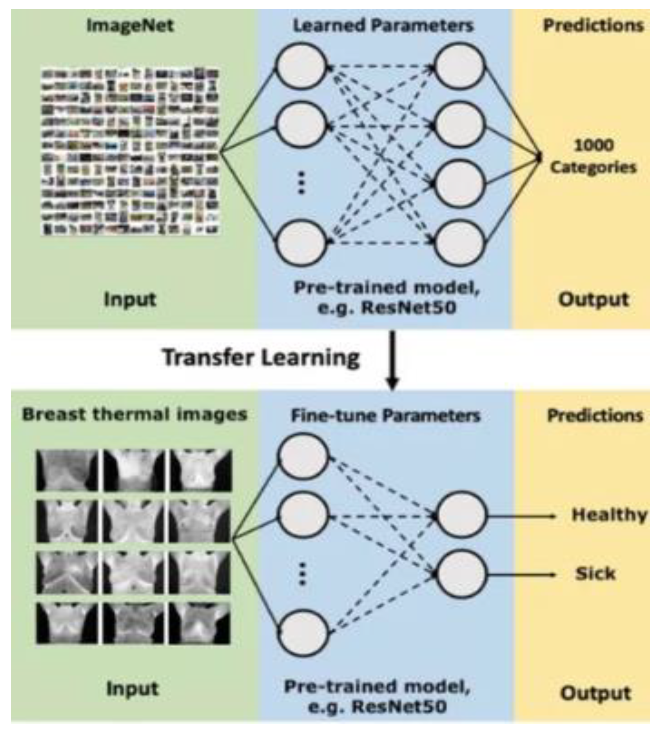
CNNs process data reminiscent of the grid processing seen in the LeNet architecture. According to [33,34], CNN consists of five data processing layers: alignment and two output layers. During the training phase, the CNN adjusts its parameters based on the provided data set, gradually increasing its accuracy [33,34,35]. Moreover, transfer learning was used to adapt an existing model to the current task, speeding up the learning process. The dataset was divided into separate subsets for training, cross-validation, and testing.
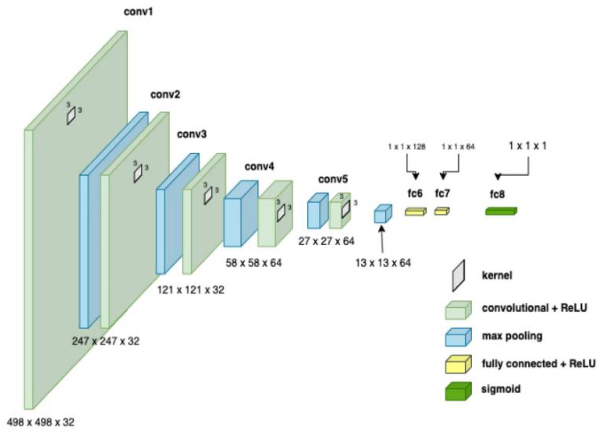
Figure 8.
Scheme of transfer learning method for binary classification.
To evaluate the models' performance eight metrics, including accuracy and precision, were used. The confusion matrix was useful in identifying areas where the model made errors.
3.5. Explainable Artificial Intelligence (XAI) Framework
Explainable Artificial Intelligence (XAI) is a subset of machine learning (ML) focused on elucidating the processes by which ML models generate their outputs. Applying XAI to an ML model enhances its reliability, as the reasoning behind the model's inferences becomes traceable [38].
Artificial Neural networks (ANN) usually comprise numerous layers linked through complex, nonlinear relationships. Even if all these layers and their interconnections were examined, it would be nearly impossible to fully understand how the ANN arrived at its decision. Consequently, deep learning is frequently regarded as a 'black box.' Given the high stakes involved in medical decision-making, it is unsurprising that medical professionals have expressed concerns about the opaque nature of deep learning, which currently represents the leading technology in medical image analysis [39,40,41,42].
There has been a demand for methods to demystify the 'black box' nature of deep learning. These methods are typically known as interpretable deep learning or explainable artificial intelligence (XAI) [38,46]. Given the high stakes in medical decision-making, it is not surprising that medical professionals have expressed concerns about the opaque nature of deep learning, which is currently the leading technology in medical image analysis [39,40,41,44].
LIME, which stands for Local Interpretable Model-Agnostic Explanations, is an algorithm designed to faithfully explain the predictions of any classifier or regressor by locally approximating it with an interpretable model. LIME offers local explanations by substituting a complex model with simpler ones in specific regions. For instance, it can approximate a CNN with a linear model by altering the input data, and then the output of the complex model changes. LIME uses the simpler model to map the relationship between the modified input data and the output changes. The similarity of the altered input to the original input is used as a weight, ensuring that explanations from the simple models with significantly altered inputs have less influence on the final explanation [45,46].
First of all, the digit classifier was built by installing tensorflow specifically employing Keras, which is installed in tensorflow. The Keras frontend simplifies the complexity of lower-level training processes, making it an excellent tool for quickly building models.
Keras includes the MNIST dataset in its distribution, which can be accessed using the load_data() method from the MNIST module. This method provides two tuples containing the training and testing data organized for supervised learning. In the code snippet, 'x' and 'y' are used to represent the images and their corresponding target labels, respectively.
The images returned by the method are 1-D numpy arrays, each with a size of 784. These images are converted from uint8 to float32 and reshaped into 2-D matrices of size 28x28. Since the images are grayscale, their pixel values range from 0 to 255. To simplify the training process, the pixel values are normalized by dividing by 255.0, which scales them between 0 and 1. This normalization step is crucial because large values can complicate the training process.
Then, a basic CNN model was developed that processes a 3-D image by passing it through Conv2D layers with 16 filters, each sized 3x3 and using the ReLU activation function. These layers learn the weights and biases of the convolution filters, essentially functioning as the "eyes" of the model to generate feature maps. These feature maps are then sent to the MaxPooling2D layer, which uses a default 2x2 max filter to reduce the dimensionality of the feature maps while preserving important features to some extent.
The basic CNN model is trained for 2 epochs with a batch size of 32 through model.fit(), and a validation set, which was set aside earlier while loading MNIST data, is used. In this context, "epochs" denotes the total number of times the model sees the entire training data, whereas "batch_size" refers to the number of records processed to compute the loss for one forward and backward training iteration.
With the model ready, LIME for Explainable AI (XAI) could be applied. The lime_image module from the LIME package is explored to create a LimeImageExplainer object. This object has an explain_instance() method that takes 3-D image data and a predictor function, such as model.predict, and provides an explanation based on the predictions made by the function.
The explanation object features a get_image_and_mask() method, which, given the predicted labels for the 3-D image data, returns a tuple of (image, mask). Here, the image is a 3-D numpy array and the mask is a 2-D numpy array that can be used with skimage.segmentation.mark_boundaries to show the features in the image that influenced the prediction.
The results of the applied algorithm will be more thoroughly presented and discussed in Result and Discussion section of the paper.
3.6. Informational Nodes for the Diagnosis
After XAI algorithms isolating the critical region of interest (ROI) (each breast separately) is isolated from the image files. At this stage, temperature data of both healthy and tumor-affected breasts, stored in spreadsheet format, are used to calculate various statistical/computational parameters. Each temperature value within the spreadsheet cell corresponds to a singular pixel from the thermal image. It is worth noting that based on available medical information, a determination is made between a healthy and an affected breast. In cases where there is no tumor, for calculations the left breast is considered affected, and the right breast is considered healthy. Temperature values are measured in degrees Celsius. Below is a complete list of parameters used for these calculations.
- Maximum Temperature
- Minimum Temperature
- Temperature Range (Maximum minus Minimum Temperature)
- Mean
- Median
- Standard deviation
- Variance
- Deviation from the Mean (Maximum minus Mean Temperature)
- Deviation from the Maximum Temperature of the Healthy Breast (Maximum minus Maximum Temperature of the Healthy Breast)
- Deviation from the Minimum Temperature of the Healthy Breast (Maximum minus Minimum Temperature of the Healthy Breast)
- Deviation from the Mean Temperature of the Healthy Breast (Maximum minus Mean Temperature of the Healthy Breast)
- Deviation between Mean Temperatures (Mean minus Mean Temperature of the Healthy Breast)
- Distance between Points of Maximum and Minimum Temperature:
- 14.
- A = Number of Pixels near the Maximum with Temperature Greater than
- 15.
- B = Number of pixels of the entire area
- 16.
- C = Number of All Pixels with Temperature Greater than
- 17.
- Ratio of A to B (A/B)
- 18.
- Ratio of C to B (C/B)
The calculated factors, along with the initially gathered patient information, are merged into a unified file format compatible with the software requirements.
3.7. Bayesian Network (BN) Model
A Bayesian network (BN), also known as a belief network or probabilistic directed acyclic graphical model, is defined mathematically as a Graph Structure and more specifically a directed Acyclic Graph (DAG), G = (V, E) where V is a set of vertices (nodes) representing random variables and E is a set of directed edges (arcs) representing conditional dependencies between the variables. Each node in the network is associated with a conditional probability distribution where are the parent nodes of in the graph G.
The main property of a BN is a theorem that simplifies the calculation of the joint probability distribution. Let be a set of n random variables represented by the nodes in the DAG, G. Then the joint probability of the set of random variables X can be factorized as:
Thus, BNs provide an efficient way to represent the joint probability distribution by exploiting conditional independencies. Inference in Bayesian networks involves computing the posterior distribution of a set of query variables given evidence about some other variables. By defining the structure and the conditional probability distributions for each node, we can model complex probabilistic relationships using Bayesian networks.
The BN models that we have constructed include as informational nodes all previously mentioned factors presented in subsection 2.6 as well as historical medical record data. Finally, we can also include as an additional factor, the diagnosis from the pure CNN model if we want.
Within the compiled data file, the diagnosis variable is integrated, where a value of 1 signifies a positive diagnosis and 0 denotes a negative one. The file is then inputted into the software (BayesiaLab 11.2.1 [47]), categorizing different parameters as either continuous or discrete (Figure 9).
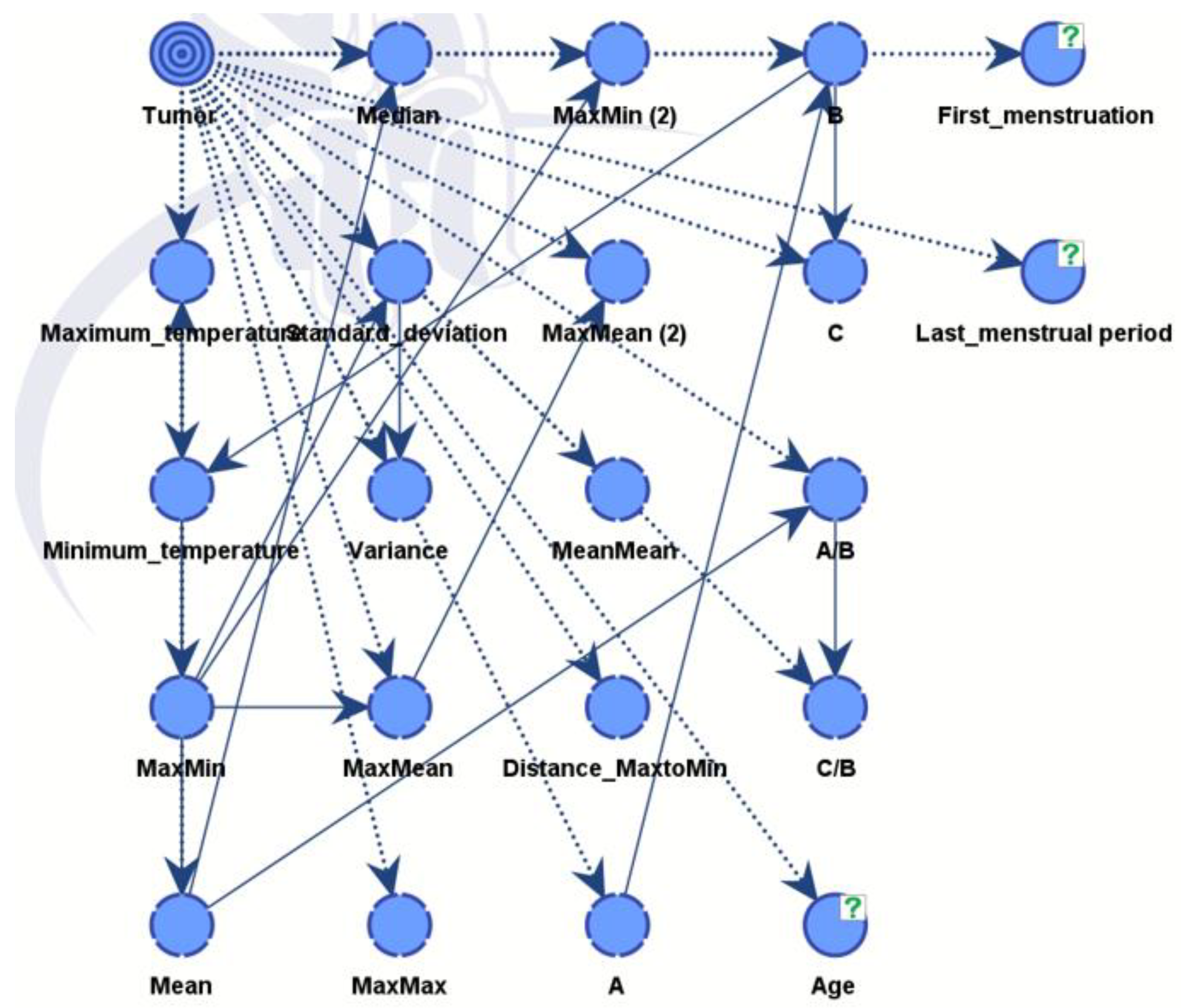
The final diagnosis decision is specifically designated as a target variable of the whole BN. Subsequently, the software computes freequencies between the provided parameters and the target variable, presenting the outcomes as conditional probabilities. Using this, the connections between nodes were established during training finalizing the acyclic graph (DAG).
Figure 10.
The link (relationship) between nodes through training in DAG.
Supervised learning, including Augmented Naive Bayes, was used to get results, and our findings were validated using K-fold analysis. In BayesiaLab, K-fold cross validation is a method used to evaluate the performance of Bayesian network models. It involves dividing the data set into K subsets (or folds), where one subset is used as the test set and the remaining K-1 subsets are used to train the model.
4. Results and Discussion
4.1. Data Compilation Results
The compiled dataset consisted of 364 images, of which 153 thermal images were categorized as “sick” and 211 thermal images were categorized as “healthy” according to the physician's diagnosis.

Table 2.
Information about the dataset.
| Healthy | Sick | Total | |
| Information gathered from a publicly accessible database [36] | 166 | 100 | 266 |
| Medical Center Astana [37] | 45 | 53 | 98 |
| Total | 211 | 153 | 364 |
Images from a total of 364 thermograms have been further processed with XAI algorithms and the factors together with patient’s medical history data were prepared for integration into Bayesialab 11.2.1 [47].
We have constructed two models. Model A suffices to discover all influential factors that drive the diagnosis from a CNN. It provides full explainability to our expert model. Model B is the final expert model that gives the best possible diagnosis.
4.2. Results of Convolutional Neural Network with XAI
XAI in this case depicted areas that contributed most when classifying images and giving them probabilities of classes Sick and Healthy. LIME library that is used to analyze images and CNN models have highlighted areas of thermal images of breast that can clearly show areas that do show movement in development of cancerous tissues. explainable parts of images are shown in Figure 11 with their respective diagnosis and classification results.
The XAI algorithm identifies the critical ROI, meaning the part of thermogram that is critical to the decision making. The model identifies in most of the cases breast regions for sick cases and the XAI doesn't identify in most cases one particular thermogram region for healthy cases.
4.3. Bayesian Network Results - Model A
Model A integrates medical record information and the factors from the thermal images that have been evaluated from critical parts of images with the help of XAI algorithm. Model B just includes also diagnostic data from a CNN model.
The combined dataset was used to train the network and evaluate its performance. The results of both models were developed and analyzed using BayesiaLab 11.2.1 software, specifically using a supervised learning approach, the Tree Augmented Naive Bayes. Additionally, the K-fold verification method did not reveal any noticeable shortcomings of the BN models, and this indicates their reliability.
In Figure 12, the nodes showed different influences and were assessed using mutual information assessment. The model displayed robustness and reliability with a dataset of 364 patients, resulting in high accuracy.
The influential factors identified were in line with data process from both unsupervised and supervised learning, as shown in Table 3.
An important measure from Table 4 is the Gini index, which reflects the equilibrium between positive and negative values of the target variable across the dataset. This equilibrium is crucial for the model to discern between the two conditions successfully and make precise predictions in both instances. An ideal Gini index, representing perfect balance, is set at 50%. In our case, the value registers at 43.04895%, which is relatively proximate to the optimal equilibrium.
Table 5 shows very good results for a XAI expert model, particularly highlighting the rates of true positives (79.5%) and true negatives (87.68%). Only 58 patients out of 364 were misclassified by the model. The model performance shown in Figure 13 below is depicted using a receiver operating characteristic (ROC) curve. The overall accuracy of the model stands at 84.07%, as shown in Table 6.
4.4. Bayesian Network with Convolutional Neural Network Results – Model B
Model B is similar to the previous model but integrates also predictions from a CNN model. The final directed acyclic graph (DAG) is presented in Figure 14. Including additional information improves performance and strengthens the model's robustness. The CNN model effectively differentiated between healthy and diseased samples, achieving an accuracy rate of 88%. Following this classification, the outcomes were integrated into the dataset for Model B.
The influential factors identified were in line with data gathered from both unsupervised and supervised learning, as shown in Table below.
Table 7.
Influence on tumor in model B.
| Node | Mutual Information | Normalized Mutual Information | Relative Mutual Information | Relative Significance | Prior Mean Value | G-test | df | p-value | G-test (Data) | df (Data) | p-value (Data) |
| CNN prediction | 0.4073 | 40.7339 | 41.4967 | 1.0000 | 0.3599 | 205.5477 | 1 | 0.0000 | 205.6822 | 1 | 0.0000 |
| Min_temperature | 0.2607 | 26.0710 | 26.5592 | 0.64000 | 29.0253 | 131.5569 | 2 | 0.0000 | 131.6458 | 2 | 0.0000 |
| Max_temperature | 0.2580 | 25.8026 | 26.2859 | 0.6334 | 34.0704 | 130.2030 | 2 | 0.0000 | 130.3019 | 2 | 0.0000 |
| Mean | 0.2251 | 22.5134 | 22.9350 | 0.5527 | 31.5695 | 113.6049 | 2 | 0.0000 | 113.6820 | 2 | 0.0000 |
| Median | 0.1999 | 19.9856 | 20.3599 | 0.4906 | 31.5530 | 100.8498 | 2 | 0.0000 | 100.9124 | 2 | 0.0000 |
| Age | 0.1860 | 18.6007 | 18.9491 | 0.4566 | 57.0016 | 93.8614 | 66 | 1.3715 | 94.4754 | 66 | 1.2300 |
| Last_menstrual period | 0.1453 | 14.5310 | 14.8032 | 0.3567 | 48.1478 | 73.3252 | 38 | 0.0503 | 87.4606 | 38 | 0.0009 |
| MaxMin | 0.0617 | 6.1739 | 6.2895 | 0.1516 | 5.0452 | 31.1542 | 2 | 0.0000 | 31.1756 | 2 | 0.0000 |
| MaxMax | 0.0423 | 4.2325 | 4.3118 | 0.1039 | 0.4620 | 21.3579 | 2 | 0.0023 | 21.3938 | 2 | 0.0023 |
| A/B | 0.0413 | 4.1279 | 4.2052 | 0.1013 | 0.0379 | 20.8299 | 2 | 0.0030 | 22.7747 | 2 | 0.0011 |
| B | 0.0383 | 3.8263 | 3.8980 | 0.0939 | 28,334.7862 | 19.3081 | 2 | 0.0064 | 19.3214 | 2 | 0.0064 |
The results are reflected in Table 8, Table 9 and Table 10, and Figure 13. Table 10 illustrates the significant improvement in model performance after integrating the CNN variable, resulting in fewer incorrect predictions. Of the 364 cases, only 33 were inaccurately diagnosed, resulting in an overall accuracy of 90.9341%. The Gini index has increased to 46.9272% due to the addition of the CNN node. In addition, the ROC index increased from 93.049% to 96.9272%.
4.5. Comparative Assessment
This section compares the performance of Model B with previous research studies that also used thermal imaging. Data was collected from various research papers using thermal imaging technology to give an idea of how Model B compares. This analysis aims to understand how well Model B performs compared to existing approaches using thermal imaging. Table 11 shows a summary of the results.
The table's comparative analysis presented Model B's performance within the context of studies focused on thermal imaging. Notably, Model B exhibits competitive accuracy with a performance of 90.9341%, which closely matches the results of several previous studies. It is worth noting that some of these previous studies may have used smaller datasets than ours, which could potentially affect the accuracy of their results. Moreover, our use of XAI integration of CNNs and BNs provides a clear advantage.
Model B in the present study has somewhat lower accuracy compared with model B of reference [35]. The reason is that we have enlarged the dataset including different sets of images with some of them of missing medical records. However, the aim of the paper is to demonstrate the efficiency of the proposed XAI methodology. It is well known that one can always achieve higher accuracy with better training based on larger and of good quality datasets.
These comparisons provide valuable information to both researchers and practitioners, guiding future developments in thermal imaging applications and highlighting ways to optimize XAI expert models’ performance in real-world scenarios.
5. Conclusion
Breast cancer continues to represent a major global health problem, highlighting the need for advanced diagnostic techniques to improve survival rates through early detection. This study extensively explored machine learning techniques, specifically Bayesian Networks (BNs), combined with Convolutional Neural Networks (CNNs) to improve intepretable early detection of breast cancer. The literature review highlights the growing burden of breast cancer and the limitations of current diagnostic methods, stimulating the study of innovative approaches. Thermography has emerged as a cost-effective and non-invasive alternative for detection.
XAI offers transparent and interpretable decision-making processes, promoting trust and collaboration between humans and artificial intelligence systems in several application domains. In the present study we have used XAI algorithms to identify the critical parts of thermal images and consequently we have integrated CNN and BN to build a highly accurate expert model for diagnosis.
The methodology included diverse datasets, facilitating the development of robust Bayesian network models for accurate breast cancer diagnosis. Using thermal images and medical records, Model A achieved an accuracy of 84.07%, while Model B, combining CNN predictions, achieved a 90.9341% accuracy. Model A has a similar performance with a sole CNN model and therefore we can trust it as a practically acceptable model that is fully readable by a physician. From Model A we can easily read the interpretation of the diagnosis. We can observe which factors are dominant as well their interactions. These results highlight the potential of machine learning methods to transform breast cancer diagnosis, improving accuracy and reducing the risk of misdiagnosis.
Moreover, the study models demonstrated competitiveness with other peer-reviewed literature articles, confirming their effectiveness and relevance. Both models performed well despite the relatively small dataset size, as confirmed by k-fold cross-validation. Future research will focus on increasing the size of the network training dataset and improving the Gini index to ensure a more balanced dataset and thereby improve performance.
In conclusion, this study contributes to advancing interpretable machine learning in healthcare by introducing innovative approaches to breast cancer detection. Successful integration of thermography, CNN, and Bayesian networks promises to improve outcomes and quality of patient care in the fight against breast cancer. Given that thermography has been cleared by the FDA only as an adjunctive tool, meaning it should only be use alongside a primary diagnostic test like mammography, not as a standalone screening or diagnostic tool, continued research and validation are thus critical to exploit these methodologies' potential.
Author Contributions
Conceptualization, M.Y.Z., V.Z. and E.Y.K.N.; methodology, Y.M., N.A. and A.M.; software, Y.M. and N.A.; validation, Y.M., N.A., V.Z. and A.M.; formal analysis, V.Z., M.Y.Z.; investigation, Y.M., N.A. and A.M.; resources, A..M., A.M..; data curation, , Y.M., N.A.; writing—original draft preparation, Y.M., N.A. and A.M.; writing—review and editing, M.Y.Z., V.Z. and E.Y.K.N; visualization, Y.M., N.A.; supervision, M.Y.Z., V.Z. and E.Y.K.N; project administration, A.M.; funding acquisition, A.M., M.Y.Z. All authors have read and agreed to the published version of the manuscript.
Funding
This research was supported by the Ministry of Science and Higher Education of the Republic of Kazakhstan AP19678197 “Integrating Physics-Informed Neural Network, Bayesian and Convolutional Neural Networks for early breast cancer detection using thermography”
Institutional Review Board Statement
The study was conducted in accordance with the Declaration of Helsinki, and approved by the Institutional Review Board (or Ethics Committee) of the Institutional Research Ethics Committee (IREC) of Nazarbayev University (identification number 775/09102023 and approval date 11/10/2023).
Data Availability Statement
Data is available at http://visual.ic.uff.br/dmi/ and https://sites.google.com/nu.edu.kz/bioengineering/dataset?authuser=0
Conflicts of Interest
The authors declare no conflicts of interest.
References
- Monticciolo D. L. et al. “Breast cancer screening recommendations inclusive of all women at average risk: update from the ACR and Society of Breast Imaging”. Journal of the American College of Radiology, 2021; Vol. 18 (9), pp. 1280-1288.
- H.-Y. Lin and J. Y. Park, “Epidemiology of cancer”, Anesthesia for Oncological Surgery, pp. 11–16, 2023. [CrossRef]
- A.N. Giaquinto, K.D. Miller, K.Y. Tossas, R.A. Winn, A. Jemal, R.L. Siegel, "Cancer statistics for African American/black people 2022," CA: Cancer J. Clin., vol. 72, no. 3, pp. 202-229, 2022.
- H. Sung et al., "Global Cancer Statistics 2020: GLOBOCAN Estimates of Incidence and Mortality Worldwide for 36 Cancers in 185 Countries," CA: A Cancer Journal for Clinicians, vol. 71, no. 3, pp. 209-249, 2021. Available: 10.3322/caac.21660.
- S. Zaheer, N. Shah, S.A. Maqbool, N.M. Soomro, "Estimates of past and future time trends in age-specific breast cancer incidence among women in Karachi, Pakistan: 2004–2025," BMC Public Health, vol. 19, pp. 1-9, 2019.
- Afaya et al., "Health system barriers influencing timely breast cancer diagnosis and treatment among women in low and middle-income Asian countries: evidence from a mixed-methods systematic review," BMC Health Serv. Res., vol. 22, no. 1, pp. 1-17, 2022.
- A.H. Farhan and M.Y. Kamil, “Texture analysis of breast cancer via LBP, HOG, and GLCM techniques,” IOP Conference Series: Materials Science and Engineering, vol. 928, no. 7, 2020. [CrossRef]
- World Health Organization (WHO). WHO—Breast Cancer: Prevention and Control. 2020. Available online: http://www.who.int/cancer/detection/breastcancer/en/index1.html (accessed on 6 February 2024).
- O. Mukhmetov et al., “Physics-informed neural network for fast prediction of temperature distributions in cancerous breasts as a potential efficient portable AI-based Diagnostic Tool,” Computer Methods and Programs in Biomedicine, vol. 242, p. 107834, Dec. 2023. [CrossRef]
- D. Tsietso, A. Yahya, and R. Samikannu. “A review on thermal imaging-based breast cancer detection using Deep Learning”. Mobile Information Systems, vol. 2022, pp. 1–19, Sep. 2022. [CrossRef]
- Grusdat, N. P., Stäuber, A., Tolkmitt, M., Schnabel, J., Schubotz, B., Wright, P. R., & Schulz, H. “Routine cancer treatments and their impact on physical function, symptoms of cancer-related fatigue, anxiety, and depression”. Supportive Care in Cancer, 2022; Vol. 30 (5), pp. 3733-3744. [CrossRef]
- M.Y. Kamil, “Computer-aided diagnosis system for breast cancer based on the Gabor filter technique,” International Journal of Electrical and Computer Engineering, vol. 10, no. 5, pp. 5235–5242, 2020. [CrossRef]
- Li, G., Hu, J., & Hu, G. “Biomarker studies in early detection and prognosis of breast cancer”. Translational Research in Breast Cancer: Biomarker Diagnosis, Targeted Therapies and Approaches to Precision Medicine, 2017; pp. 27-39. ISBN: 978-981-10-6019-9.
- P.N. Pandey, N. Saini, N. Sapre, D.A. Kulkarni, and D.A.K. Tiwari. “Prioritising breast cancer theranostics: a current medical longing in oncology”. Cancer Treatment and Research Communications, vol. 29, 2021. [CrossRef]
- G. Jacob, I. Jose. “Breast cancer detection: A comparative review on passive and active thermography”. Infrared Physics & Technology, vol. 134, p. 104932, Nov. 2023. [CrossRef]
- S.G. Kandlikar, I. Perez-Raya, P.A. Raghupathi, J.-L. Gonzalez-Hernandez, D. Dabydeen, L. Medeiros, P. Phatak. “Infrared imaging technology for breast cancer detection–Current status, protocols and new directions”. Int. J. Heat Mass Transfer, vol. 108, pp. 2303-2320, 2017.
- B.A. Zeidan, P.A. Townsend, S.D. Garbis, E. Copson, R.I. “Cutress. Clinical proteomics and breast cancer”. Surgeon, vol. 13, no. 5, pp. 271–278, 2015. [CrossRef]
- Yoen, H., Jang, M. J., Yi, A., Moon, W. K., & Chang, J. M. “Artificial intelligence for breast cancer detection on mammography: factors related to cancer detection”. Academic Radiology, 2024. [CrossRef]
- P.E. Freer, “Mammographic breast density: Impact on breast cancer risk and implications for screening,” RadioGraphics, vol. 35, no. 2, pp. 302–315, Mar. 2015. [CrossRef]
- M.H. Alshayeji, H. Ellethy, S. Abed, and R. Gupta, “Computer-aided detection of breast cancer on the Wisconsin dataset: an artificial neural networks approach,” Biomedical Signal Processing and Control, vol. 71, 2022. [CrossRef]
- Mashekova, Y. Zhao, E.Y. Ng, V. Zarikas, S.C. Fok, and O. Mukhmetov, "Early detection of breast cancer using infrared technology–A comprehensive review," Therm. Sci. Eng. Prog., vol. 27, article 101142, 2022.
- M.B. Rakhunde, S. Gotarkar, and S.G. Choudhari, "Thermography as a breast cancer screening technique: A review article," Cureus, vol. 14, no. 11, 2022.
- P. P. R. Pavithra, R. K. S. Ravichandran, S. K. R. Sekar, and M. R. Manikandan. “The effect of thermography on breast cancer detection-A survey,” Systematic Reviews in Pharmacy, vol. 9, no. 1, pp. 10–16, Jul. 2018. [CrossRef]
- F. AlFayez, M.W.A. El-Soud, and T. Gaber, "Thermogram breast cancer detection: A comparative study of two machine learning techniques," Appl. Sci., vol. 10, no. 2, p. 551, 2020.
- Rai, Hari Mohan, and Joon Yoo. "A comprehensive analysis of recent advancements in cancer detection using machine learning and deep learning models for improved diagnostics." Journal of Cancer Research and Clinical Oncology 149, no. 15 (2023): 14365-14408.
- Ukiwe, E. K., Adeshina, S. A., Jacob, T., & Adetokun, B. B. “Deep learning model for detection of hotspots using infrared thermographic images of electrical installations”. Journal of Electrical Systems and Information Technology, 2024, 11(1), 24.
- Raghavan, K., Balasubramanian, S. and Veezhinathan, K. “Explainable artificial intelligence for medical imaging: Review and experiments with infrared breast images”. Computational Intelligence, 2024, 40(3), p.e12660.
- Husaini MASA, Habaebi MH, Hameed SA, Islam MR, Gunawan TS. “A systematic review of breast cancer detection using thermography and neural networks”. IEEE Access. 2020; 8:208922–37. [CrossRef]
- Hakim A, Awale RN. “Thermal imaging—an emerging modality for breast cancer detection: a comprehensive review”. J Med Syst. 2020; 44 (136):10. [CrossRef]
- Ibeni, W. N. L. W. H., Salikon, M. Z. M., Mustapha, A., Daud, S. A., & Salleh, M. N. M. “Comparative analysis on bayesian classification for breast cancer problem”. Bulletin of Electrical Engineering and Informatics, 2019; Vol. 8 (4), pp. 1303-1311. [CrossRef]
- Nicandro CR, Efrén MM, Yaneli AAM, Enrique MDCM, Gabriel AMH, Nancy PC, Alejandro GH, Guillermo de Jesús HR, Erandi BMR. “Evaluation of the diagnostic power of thermography in breast cancer using Bayesian network classifiers”. Comput. Math Methods Med. 2013; 13:10. [CrossRef]
- Ekicia S, Jawzal H. “Breast cancer diagnosis using thermography and convolutional neural networks”. Med Hypotheses. 2020; 137:109542. [CrossRef]
- Aidossov, N., Mashekova, A., Zhao, Y., Zarikas, V., Ng, E. and Mukhmetov, O. “Intelligent Diagnosis of Breast Cancer with Thermograms using Convolutional Neural Networks”. In Proceedings of the 14th International Conference on Agents and Artificial Intelligence (ICAART 2022) – Vol. 2, pp. 598-604. [CrossRef]
- Aidossov, N., Zarikas, V., Zhao, Y. et al. “An Integrated Intelligent System for Breast Cancer Detection at Early Stages Using IR Images and Machine Learning Methods with Explainability”. SN COMPUT. SCI. 4, 184 (2023). [CrossRef]
- Aidossov, N.; Zarikas, V.; Mashekova, A.; Zhao, Y.; Ng, E.Y.K.; Midlenko, A.; Mukhmetov, O. “Evaluation of Integrated CNN, Transfer Learning, and BN with Thermography for Breast Cancer Detection”. Appl. Sci. 2023, 13, 600. [CrossRef]
- Visual Lab DMR Database. Available online: http://visual.ic.uff.br/dmi/ (accessed in November 2022).
- Thermogram dataset (2023). Available at: https://sites.google.com/nu.edu.kz/bioengineering/dataset?authuser=0 (Access: January, 2024).
- Adadi, A., Berrada, M. “Peeking Inside the Black-Box: A Survey on Explainable Artificial Intelligence (XAI)”. IEEE, 2018; Access 6, 52138–52160. [CrossRef]
- Jia, X., Ren, L., Cai, J. “Clinical implementation of AI technologies will require interpretable AI models”. Med. Phys., 2020; 47, 1–4. [CrossRef]
- Litjens, G., Kooi, T., Bejnordi, B.E., Setio, A.A.A., Ciompi, F., Ghafoorian, M., van der Laak, J.A.W.M., van Ginneken, B., Sánchez, C.I., 2017. “A survey on deep learning in medical image analysis”. Med. Image Anal., 2017. [CrossRef]
- Meijering, E. “A bird’s-eye view of deep learning in bioimage analysis”. Comput. Struct. Biotechnol. J., 2020. [CrossRef]
- Shen, D., Wu, G., Suk, H.I. “Deep learning in medical image analysis”. Annu. Rev. Biomed. Eng., 2017; 19, 221–248. [CrossRef]
- Murdoch, W.J., Singh, C., Kumbier, K., Abbasi-Asl, R., Yu, B. “Definitions, methods, and applications in interpretable machine learning”. Proc. Natl. Acad. Sci. USA, 2019; 116, 22071–22080. [CrossRef]
- Shen, S., Han, S.X., Aberle, D.R., Bui, A.A., Hsu, W. “An interpretable deep hierarchical semantic convolutional neural network for lung nodule malignancy classification”. Expert Syst. Appl. 2019; 128, 84–95. [CrossRef]
- Ribeiro, M.T., Singh, S., Guestrin, C. “Why should I trust you?” Explaining the predictions of any classifier. In: Proceedings of the ACM SIGKDD International Conference on Knowledge Discovery and Data Mining. Association for Computing Machinery, New York, New York, USA, 2016; pp. 1135–1144. [CrossRef]
- Malhi, A., Kampik, T., Pannu, H., Madhikermi, M., Framling, K., 2019. Explaining machine learning-based classifications of in-vivo gastral images. In: Proceedings of the International Conference on Digital Image Computing: Techniques and Applications, DICTA doi:10.1109/DICTA47822.2019.8945986, 2019. Institute of Electrical and Electronics Engineers Inc., Department of Computer Science, Aalto University Finland, Finland.
- Bayesia Lab (2001). Computer program. Available at: https://www.bayesia.com/ (Downloaded: September 2023).
- M. de F. O. Baffa and L. G. Lattari, “Convolutional neural networks for static and Dynamic Breast Infrared Imaging Classification,” 2018 31st SIBGRAPI Conference on Graphics, Patterns and Images (SIBGRAPI), Oct. 2018. [CrossRef]
- J. C. Torres-Galván et al., “Deep convolutional neural networks for classifying breast cancer using infrared thermography,” Quantitative InfraRed Thermography Journal, vol. 19, no. 4, pp. 283–294, May 2021. [CrossRef]
- Y.-D. Zhang et al., “Improving ductal carcinoma in situ classification by convolutional neural network with exponential linear unit and rank-based weighted pooling,” Complex & Intelligent Systems, vol. 7, no. 3, pp. 1295–1310, Nov. 2020. [CrossRef]
- M. A. Farooq and P. Corcoran, “Infrared Imaging for human thermography and breast tumor classification using thermal images,” 2020 31st Irish Signals and Systems Conference (ISSC), Jun. 2020. [CrossRef]
Figure 1.
Thermographic images: (a) image of healthy patient, (b) omage of sick image.
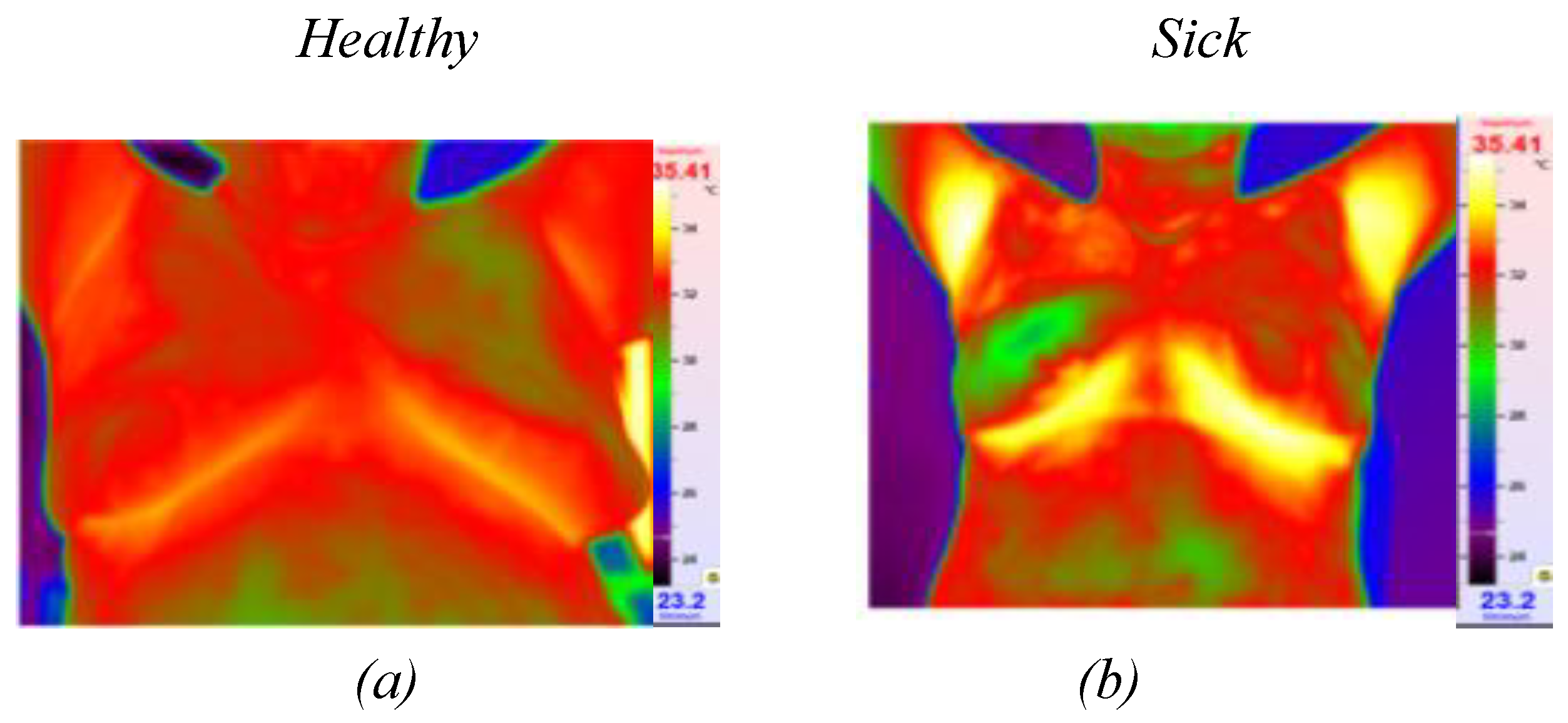
Figure 2.
Thermal imaging cameras: (a) IRTIS 2000ME, (b) FLUKE TiS60+.
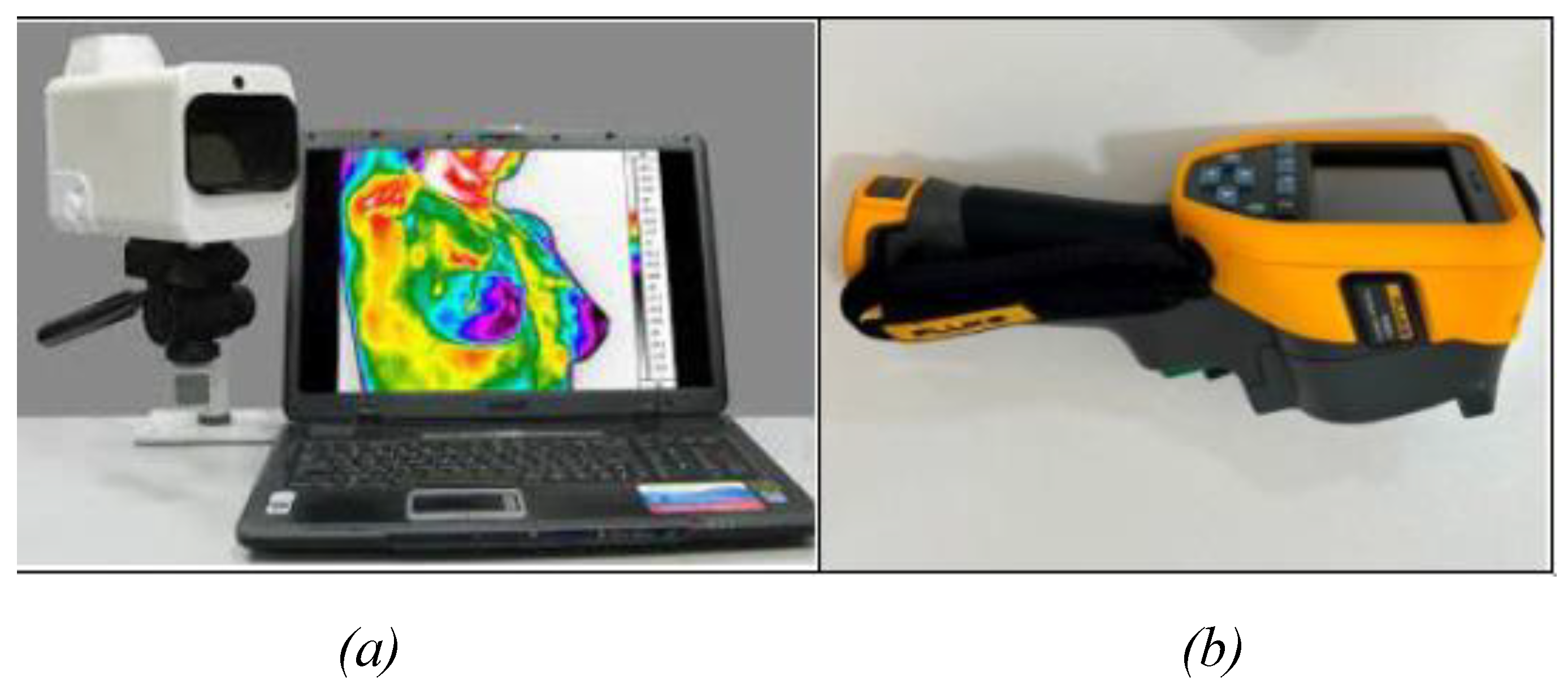
Figure 3.
Diagram for detecting breast abnormalities using thermography.
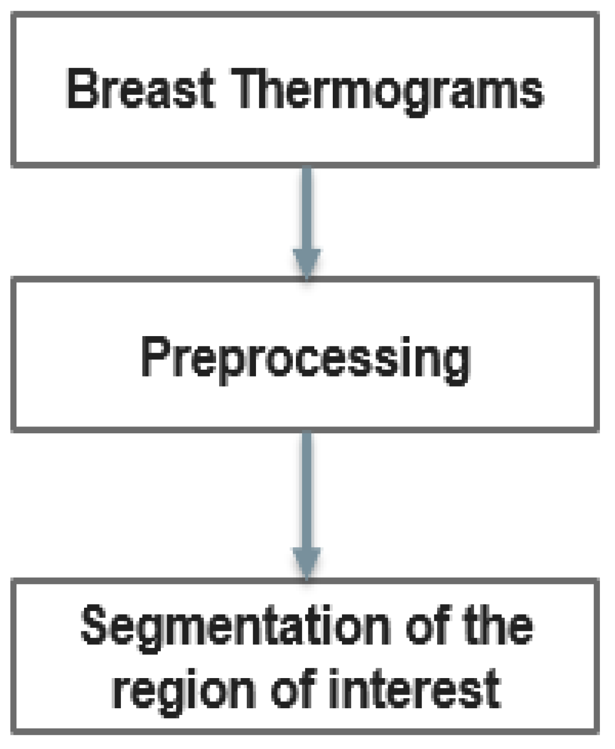
Figure 4.
Transforming thermal images into an array of temperature values per pixel.
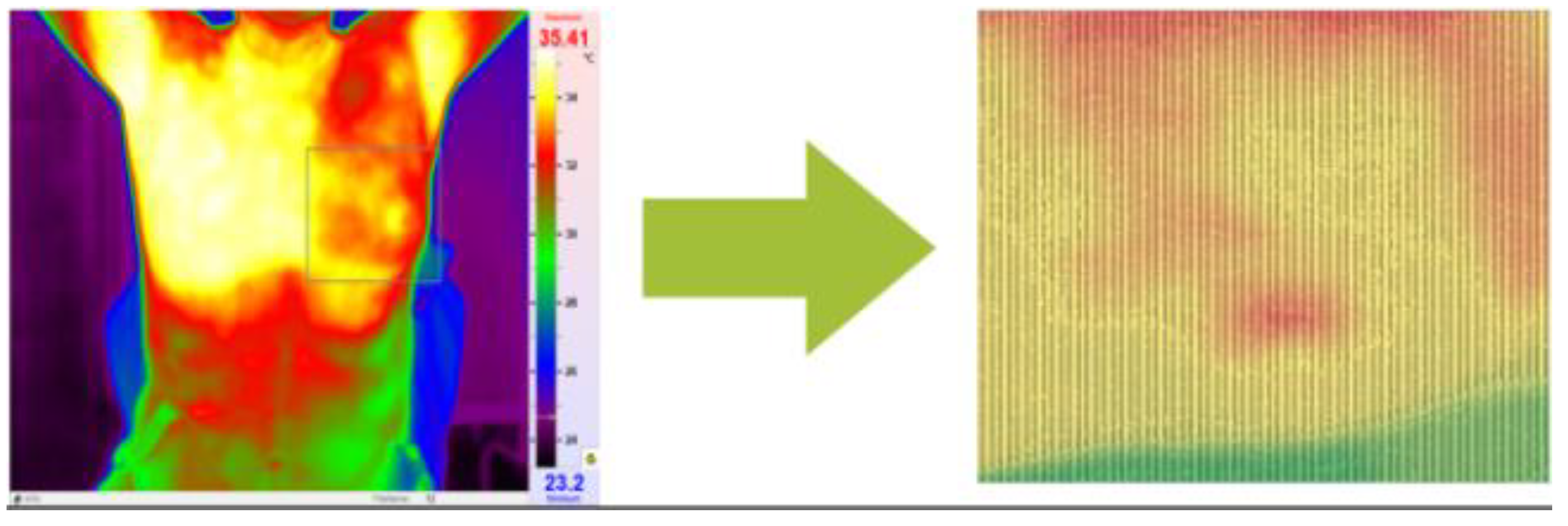
Figure 5.
Python code of the proposed model
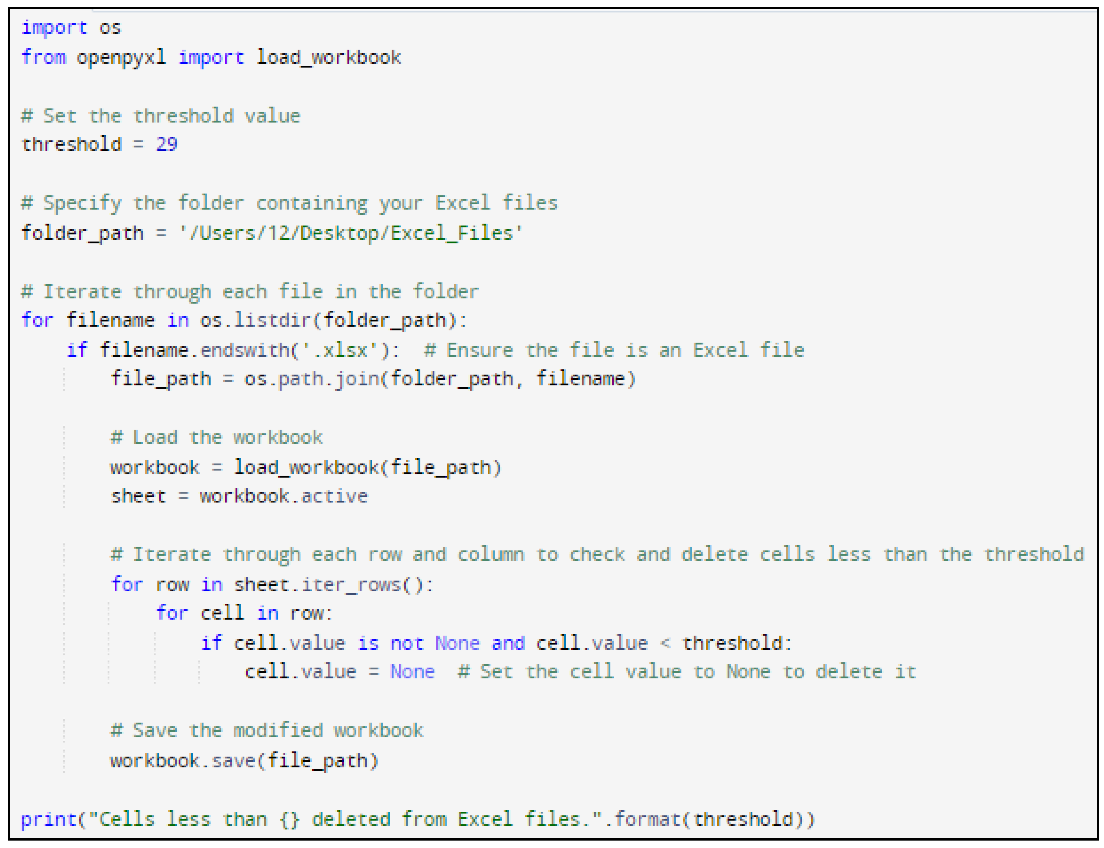
Figure 6.
Result of the segmentation.
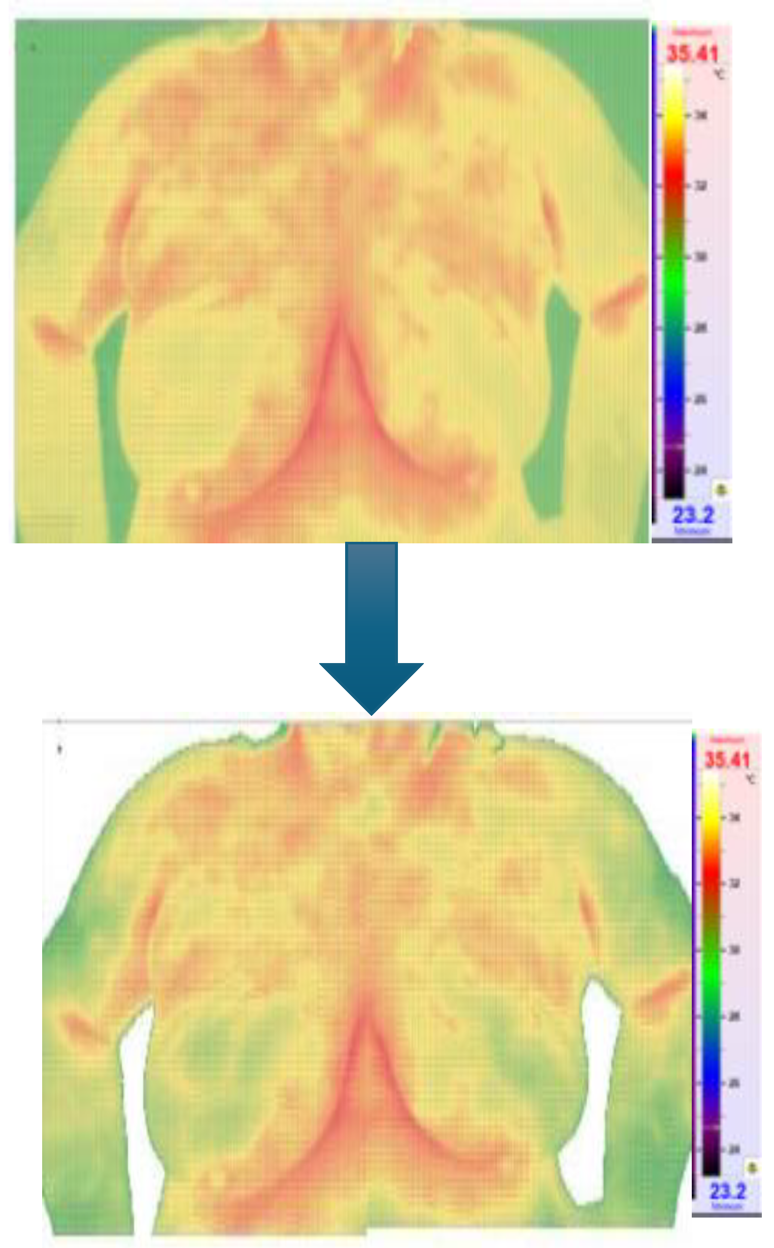
Figure 9.
Definition of Variables (Continuous/Discrete).
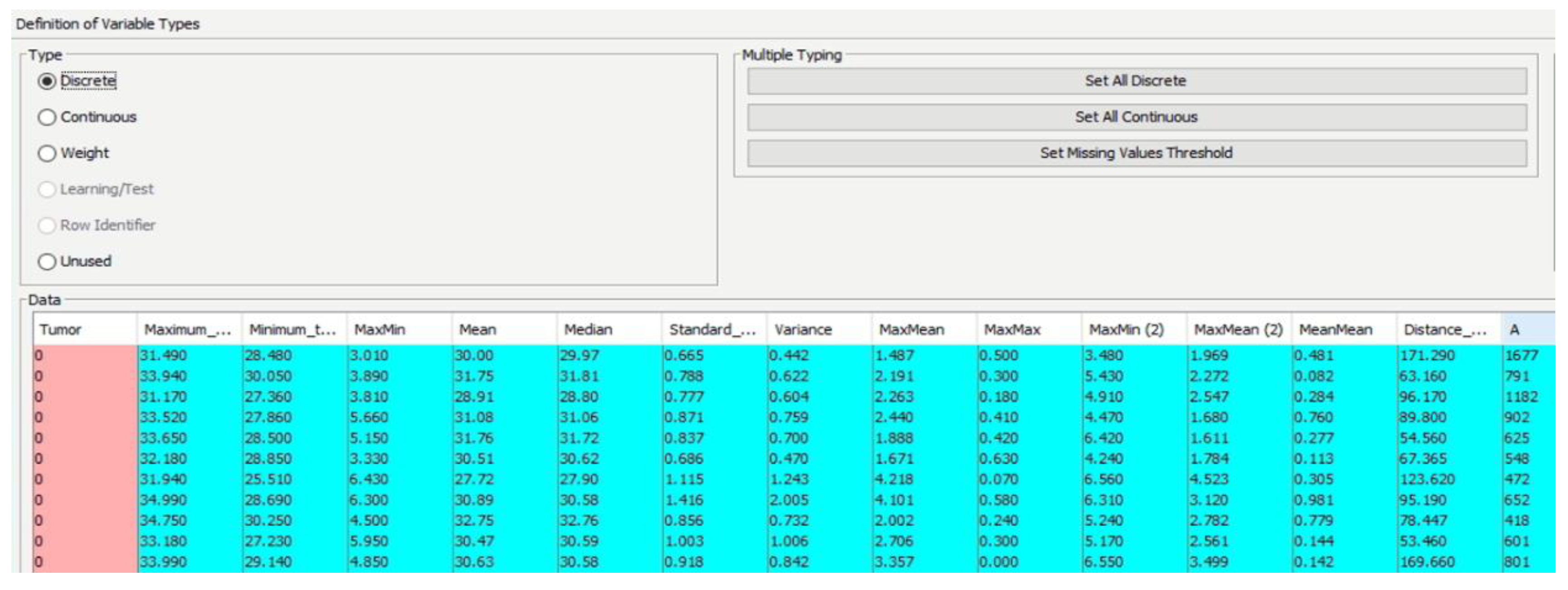
Figure 11.
Highlighted areas of image by XAI library that shows parts which contributed for CNN to make decision.
Figure 11.
Highlighted areas of image by XAI library that shows parts which contributed for CNN to make decision.
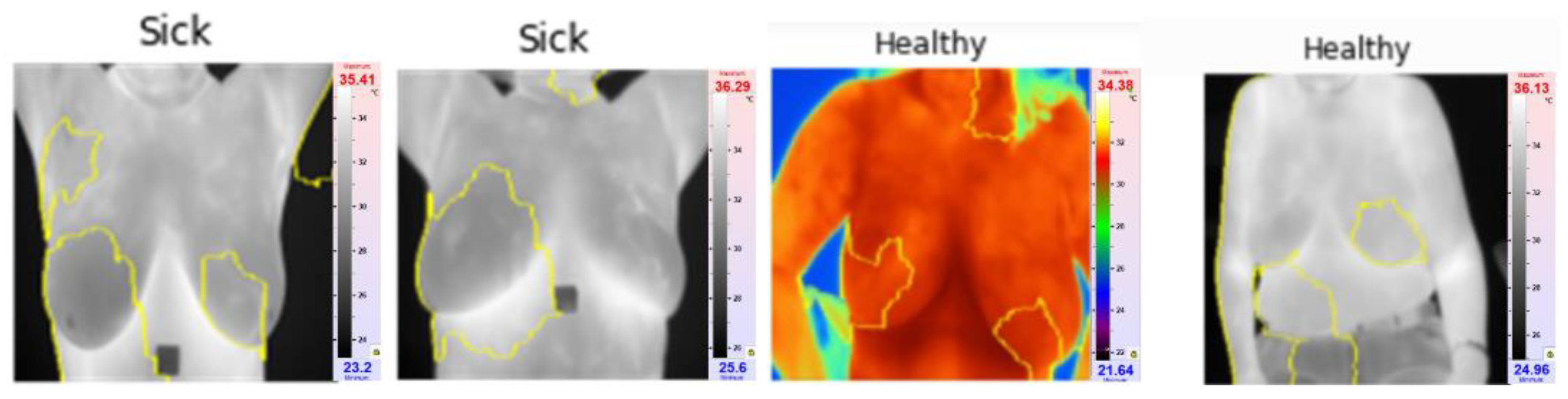
Figure 12.
Model A and Factors Influencing the Tumor Target Variable.
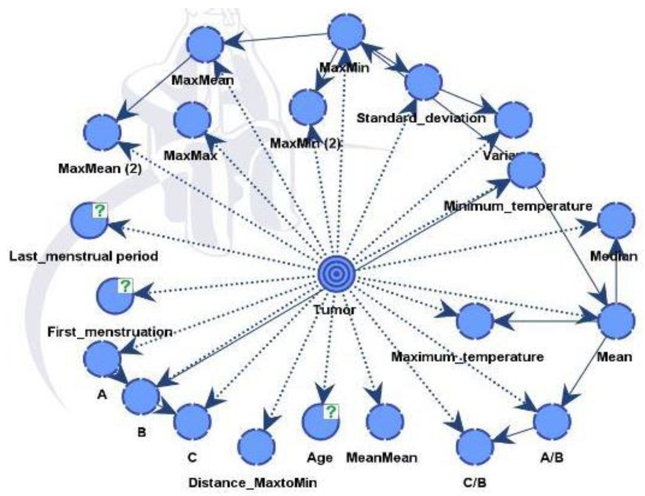
Figure 13.
ROC Curve for Model A and Model B.
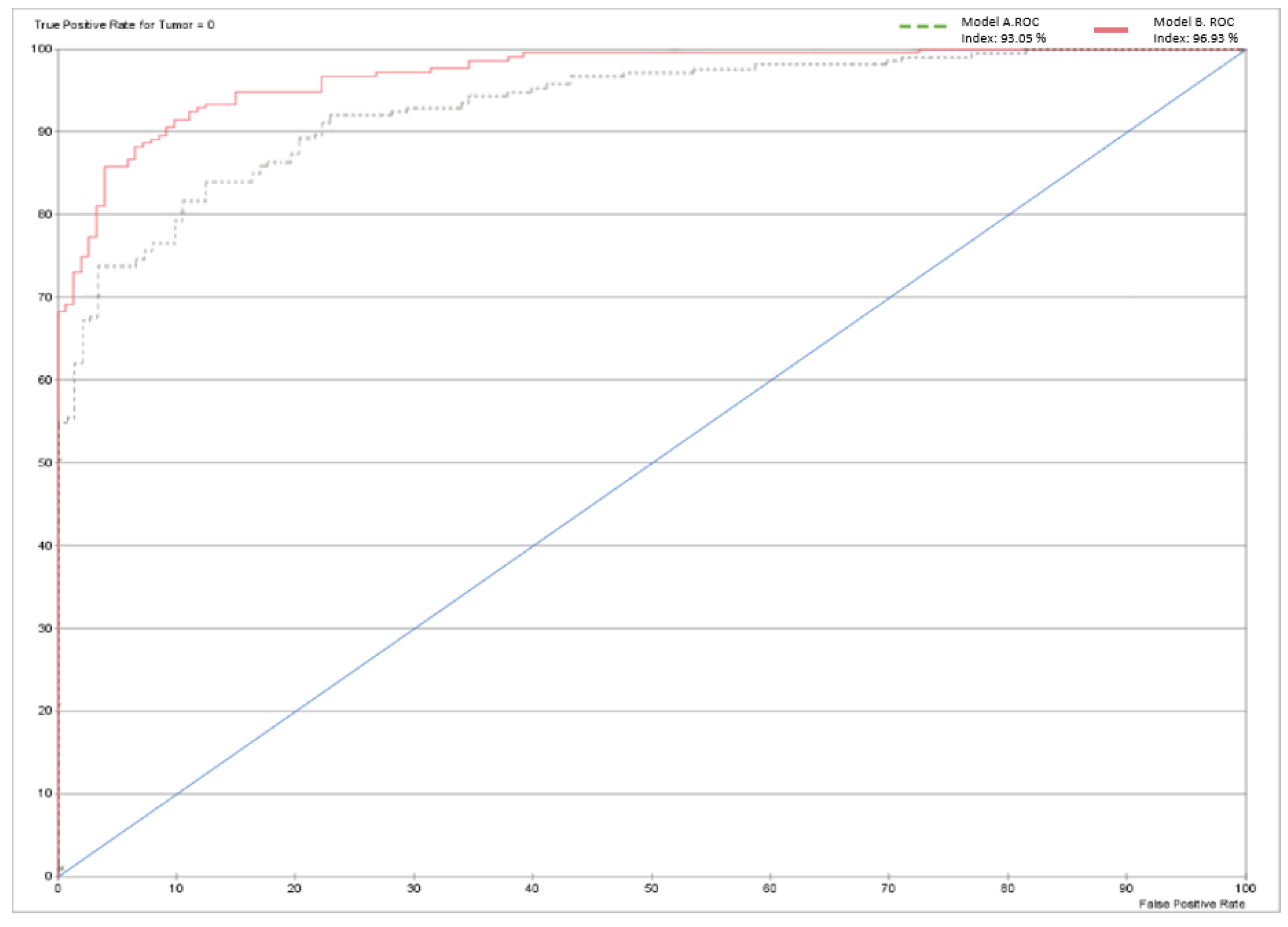
Figure 14.
Model B and Factors Influencing the Tumor Target Variable.
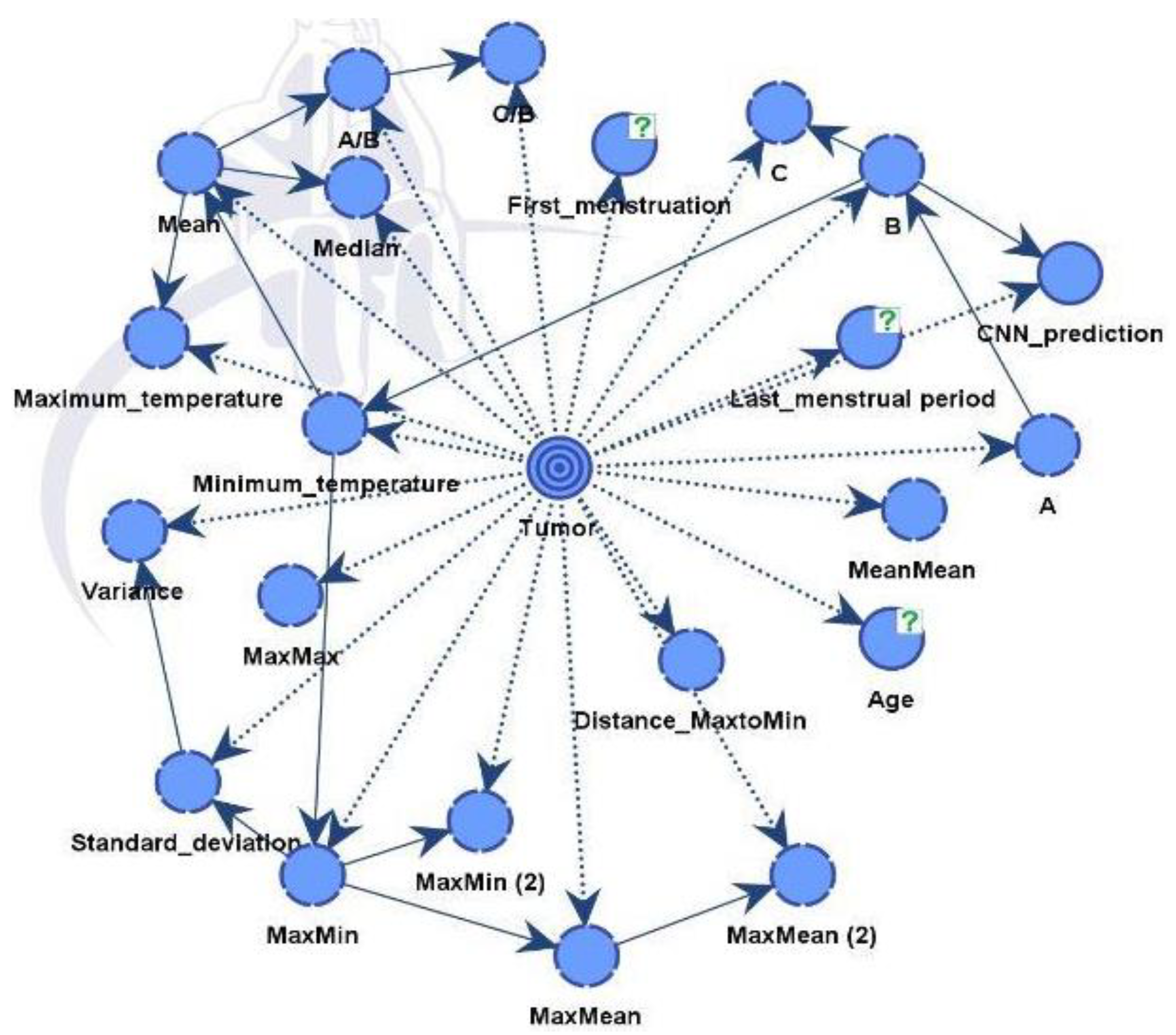
Table 1.
Evaluation of current breast cancer detection methodologies.
| Methods | Radiation | Sensitivity | Tumor size | Advantage | Disadvantage |
| Mammography | X-rays | 84% | ≤2 cm | Simultaneous screening of bone, soft tissues, and blood vessels on a mass scale | Preferentially chosen for individuals above 40 years old due to considerations regarding the impact of ionizing radiation |
| Ultrasound | Sound waves | 82% | 2 cm | Affordable evaluation of breast lumps with safety considerations | Low resolution |
| Magnetic Resonance Imaging (MRI) | RF Waves | 95% | ≤2 cm | Non-invasive and safe | The reconstruction process encounters an ill-posed problem |
| Thermography | No radiation | 85% | 1 cm | Cost-effective, non-invasive, and safe | Limited in its ability to detect tumors located deeper within the body |
| Computer Tomography (CT) | Ionizing radiation | 81.2% | 1 cm | Non-invasive, powerful to create clear images on the computer, does not depend on density of the breast | X-ray exposure, expensive, limited accessibility |
Table 3.
Influence on tumor in model A.
| Node | Mutual Information | Normalized Mutual Information | Relative Mutual Information | Relative Significance | Prior Mean Value | G-test | df | p-value | G-test (Data) | df (Data) | p-value (Data) |
| Max_Temperature | 0.2648 | 26.4847 | 26.9807 | 1.0000 | 34.0704 | 133.6448 | 2 | 0.0000 | 133.7700 | 2 | 0.0000 |
| Mean | 0.2173 | 21.7323 | 22.1393 | 0.8206 | 31.5696 | 109.6638 | 2 | 0.0000 | 109.7311 | 2 | 0.0000 |
| Median | 0.2135 | 21.3515 | 21.7514 | 0.8062 | 31.5531 | 107.7421 | 2 | 0.0000 | 107.8073 | 2 | 0.0000 |
| Min_temperature | 0.1881 | 18.8055 | 19.1577 | 0.7101 | 29.0253 | 94.8947 | 2 | 0.0000 | 94.9764 | 2 | 0.0000 |
| Age | 0.1860 | 18.6007 | 18.9491 | 0.7023 | 57.0016 | 93.8614 | 66 | 1.3715 | 94.4754 | 66 | 1.2300 |
| Last_menstrual period | 0.1453 | 14.5310 | 14.8032 | 0.5487 | 48.1478 | 73.3252 | 38 | 0.0503 | 87.4606 | 38 | 0.0009 |
| B | 0.0522 | 5.2226 | 5.3204 | 0.1972 | 28,337.8891 | 26.3539 | 2 | 0.0002 | 26.5726 | 2 | 0.0002 |
| MaxMax | 0.0450 | 4.4994 | 4.5837 | 0.1699 | 0.4621 | 22.7045 | 2 | 0.0012 | 22.8927 | 2 | 0.0011 |
| MaxMin | 0.0314 | 3.1357 | 3.1944 | 0.1184 | 5.0454 | 15.8229 | 2 | 0.0367 | 15.8454 | 2 | 0.0362 |
| A/B | 0.0223 | 2.2306 | 2.2724 | 0.0842 | 0.0369 | 11.2559 | 2 | 0.3596 | 11.2609 | 2 | 0.3587 |
Table 4.
Performance Summary of Model A.
| Target: Tumor | |
| Gini Index | 43.04895% |
| Relative Gini Index | 86.0979% |
| Lift index | 1.62245 |
| Relative Lift Index | 95.31725% |
| ROC Index | 93.049% |
| Calibration Index | 89.19985% |
Table 5.
Model A Confusion Table
| Occurrences | ||
| Value | 0 (211) | 1 (153) |
| 0 (203) | 178 | 25 |
| 1 (161) | 33 | 128 |
| Reliability | ||
| Value | 0 (211) | 1 (153) |
| 0 (203) | 87.6847% | 12.3153% |
| 1 (161) | 20.4969% | 79.5031% |
| Precision | ||
| Value | 0 (211) | 1 (153) |
| 0 (203) | 84.3602% | 16.3399% |
| 1 (161) | 15.6398% | 83.6601% |
Table 6.
Overall Accuracy of Model A
| Classification Statistics | |
| Overall Precision | 84.0659% |
| Mean Precision | 84.0102% |
| Overall Reliability | 84.2457% |
| Mean Reliability | 83.5939% |
Table 8.
Performance Summary of Model B.
| Target: Tumor | |
| Gini Index | 46.9272% |
| Relative Gini Index | 93.8544% |
| Lift index | 1.67005 |
| Relative Lift Index | 98.02405% |
| ROC Index | 96.9272% |
| Calibration Index | 88.3618% |
Table 9.
Model B Confusion Table.
| Occurrences | ||
| Value | 0 (211) | 1 (153) |
| 0 (203) | 195 | 17 |
| 1 (161) | 16 | 136 |
| Reliability | ||
| Value | 0 (211) | 1 (153) |
| 0 (203) | 91.9811% | 8.0189% |
| 1 (161) | 10.5263% | 89.4737% |
| Precision | ||
| Value | 0 (211) | 1 (153) |
| 0 (203) | 92.4171% | 11.1111% |
| 1 (161) | 7.5829% | 88.8889% |
Table 10.
Overall Accuracy of Model B.
| Classification Statistics | |
| Overall Precision | 90.9341% |
| Mean Precision | 90.6530% |
| Overall Reliability | 90.9272% |
| Mean Reliability | 90.7274% |
Disclaimer/Publisher’s Note: The statements, opinions and data contained in all publications are solely those of the individual author(s) and contributor(s) and not of MDPI and/or the editor(s). MDPI and/or the editor(s) disclaim responsibility for any injury to people or property resulting from any ideas, methods, instructions or products referred to in the content. |
© 2024 by the authors. Licensee MDPI, Basel, Switzerland. This article is an open access article distributed under the terms and conditions of the Creative Commons Attribution (CC BY) license (http://creativecommons.org/licenses/by/4.0/).
Copyright: This open access article is published under a Creative Commons CC BY 4.0 license, which permit the free download, distribution, and reuse, provided that the author and preprint are cited in any reuse.


