Submitted:
03 September 2024
Posted:
04 September 2024
You are already at the latest version
Abstract
Short-circuit blowing is an important technical means to ensure the rapid surfacing of submersible. In order to study the impact of seven multiple manipulation factors of three levels on blowing, a proportional short-circuit blowing model test bench had been built and L18(37) orthogonal experiments were carried out; then, using Back propagation neural network and Pearson correlation analysis, the experimental data were trained and predicted, correlation between individual factor and blowing was further studied as supplement of orthogonal experiments. It had been proved that both multi-factor combination and individual including blowing duration, sea tank back pressure, the gas blowing pressure of the cylinder group, and sea valve flowing area had larger influence, whose correlation coefficients were 0.6535, 0.8105, 0.5569, 0.5373, of which the F-ratio of blowing duration is over critical value 3.24. And statistical evaluation indicators of Back propagation neural network were between 10e-2 and 10e-13, relative error was less than 3%, and prediction error accuracy was 100%. Based on the results above, a reasonable prediction method for submersible short-circuit blowing had been formed and suggestions on engineering design and operations were proposed, including advantage of short-circuit blowing method, initial condition settings and manipulation strategy.
Keywords:
submersible
; proportional short-circuit blowing model
; orthogonal experiments
; statistical researching methods
; back propagation neural network
; statistical evaluation indicator
; pearson correlation method
1. Introduction
In recent years, the navigational safety of submersibles has received increasing and widespread attentions. High-pressure blowing is one of the critical means to ensure the submersible surfacing. Among them, rudder jam under high-speed navigation and emergency disposal when compartment is flooding are the two most common applications [1]. Short-circuit blowing, specifically refers to an effective way to blow off ballast tanks directly with compressed gas from the cylinder group without passing through the gas distribution mechanism, of which the blowing efficiency depends on many manipulation factors including gas pressure and volume of high-pressure gas cylinder group [2].At present, the main methods to study short-circuit blowing include mathematical modeling, numerical calculations and real ship or bench experiments.
In the field of mathematical modeling and numerical calculations,CFD method was used to study the formation and evolution of the gas-liquid two-phase interface in the ballast tank during short-circuit blowing, and deeply analyzed the change process of discharge rate [1]. Several studies in this field had considered individual manipulation factor including flowing area of sea valve [3], outboard back pressure, high-pressure cylinder group gas pressure and cylinder volume [4], and gas or water supply pipeline[5]. With the help of Laval nozzle theory, an emergency surfacing motion model of submersible including short-circuit blowing was established and water ingress restriction line in underwater maneuverability safety boundary diagram was further deduced [6]. In summary, those studies above lack specific experimental evaluations and universality because of ignoring entire manipulation factors, so they can not reflect the physics principle of short-circuit blowing thoroughly.
In the field of real ship or bench experiments, an emergency short-circuit blowing test on a Spanish S-80 submarine had been conducted with an instantaneous blowing gas pressure up to 25MPa, which was equivalent as 2500m depth of outboard back pressure and too dangerous [7]. Small-scale emergency gas jet blowing-off bench experiments had been carried out, simulating the blowing and drainage performance at a depth of 100m, which had acquired relative errors of 5% and 10% of drainage percentage individually [8,9]. Experiments of small-scale short-circuit blowing test bench had been carried out, evaluating the physics principle of Laval nozzle theory and acquiring the relative errors of 8% of flowing-rate of high-pressure gas cylinder group, which was highly related with the drainage percentage of ballast tank [10,11]. For the real ship experiments, although the data was highly credible, but it is too risky. While the small scale bench experiments could be used to verify theoretical models, but due to the restriction of scale effect, the results still lacked significant guidings for real ship manipulations or engineering designs. However, proportional short-circuit blowing model experiment is a method to study the performance of short-circuit blowing of real-ship, the test bench had simulated the process of gas cylinder deflation and ballast tank drainage to analyze the influencing effects of gas cylinder group volume and gas pressure, sea valve flowing area on the blowing efficiency, obtaining the relative error of gas peak pressure of ballast tank, which was below 15% when the high pressure gas pressure of gas cylinder was under 15MPa [2]. Comparing with real ship short-circuit blowing, it couldn’t cover whole range of working conditions, and had ignored several key manipulation factors including outboard back pressure, length and inner diameter of gas supply pipeline, and blowing duration.
The researches above can be briefly concluded as below:

Table 1.
Recent Researches on short-circuit blowing or related field.
| Researching Field | Methodology | Disadvantage |
|---|---|---|
| Mathematical modeling | Short-circuit blowing in center of Laval nozzle theory [6]. | Lacking specific experimental evaluations and universality because of ignoring entire manipulation factors. |
| Gas-liquid two-phase interface evolution modeling of blowing [1]. | ||
| Simulation considering flowing area of sea valve of blowing [3]. | ||
| Simulation considering outboard back pressure, high-pressure cylinder group gas pressure and cylinder volume of blowing [4]. | ||
| Simulation considering the gas or water supply pipeline [5]. | ||
| Real ship or bench experiments | Emergency short-circuit blowing test on a Spanish S-80 submarine [7]. | Too risky. |
| Experiments considering the depth of 100m [8,9]. | Restriction of scale effect. | |
| Experiments of small-scale short-circuit blowing test bench [10,11]. | ||
| Experiments of proportional short-circuit blowing model test [2]. | Incomplete working conditions, ignoring entire manipulation factors. |
In this paper, in aim of studying the influencing of more manipulation factors on blowing, our contributions are fourfold:
- First, in section 2, seven detailed influencing factors of 3 levels of high pressure short-circuit blowing were further considered in and corresponding proportional model test bench had been built, L18(37) orthogonal experiments were carried out.
- Second, in section 3, by analysis of extreme variance and variance, the correlation coefficients of blowing duration, sea tank back pressure, gas blowing pressure of the cylinder group, and sea valve flowing area were 0.6535, 0.8105, 0.5569, 0.5373, of which the F-ratio of blowing duration is over critical value 3.24.
- Third, in section 4.1, the orthogonal experimental data had been trained by Back propagation Neural Network, of which the statistical indicators were between 10e-2 and 10e-13, the relative errors of prediction was less than 3%, and the prediction error accuracy was 100%.
- Fourth, in section 4.2, through Pearson correlation analysis based on orthogonal experimental data, the correlation coefficient between individual factor and blowing had been explored, forming in-depth supplements to the conclusions of orthogonal experiments.
2. Proportional Short-Circuit Blowing Model Test Bench and Orthogonal Experiments Design
A Proportional Short-circuit blowing model test bench had been constructed, basing on real-ship parameters and investigating the effects of multiple manipulation factors of different levels on blowing through orthogonal experiments.
2.1. Detailed Setup of Model Test Bench
The bench included gas cylinder group, air compressor, high-pressure gas cylinder group and gas distribution mechanism, sea tank and ballast tank. Among these, ballast water tank and sea tank were set between sea valves of different diameters. The air compressor inflates the gas cylinder group, and at the same time inflates the top of the sea tank to form back pressure. When blowing started, the gas of cylinder group flew into the ballast tank through the gas supply pipeline, discharging the water into the sea tank through sea valve. The diagram of proportional short-circuit blowing test bench of submersible had been shown in Figure 1, whose main parameters had been shown in Table 2.
2.2. Orthogonal Experiment Design
Compared with test bench of reference [2], the manipulation factors of this bench included gas cylinder group volume and pressure, gas supply pipeline length, sea valve inner diameter, blowing duration, gas supply pipeline inner diameter and sea tank back pressure, each factor with three levels. According to principle of permutation and combination, there are totally 37=2187 experiments which is a huge number.
Orthogonal experimental method is an efficient, fast and economical evaluation method, especially suitable for multi factors of various level. By reasonably selecting the orthogonal experiments, more accurate and reliable results can be obtained with fewer trials [12]. In this bench, constructing orthogonal experiment table L18(37), 3 is the number of levels, 7 is the number of factors, 18 is the number of experiments, which were shown in Table 3. The ballast tank drainage percentage was selected to measure the blowing effect, seven manipulation factors were represented by A, B, C, D, E, F, G, and three levels were represented by 1, 2, 3 respectively as follows: A represents the gas cylinder group volume, three levels of 1-250L/2-500L/3-750L; B represents the length of the gas supply pipeline, three levels of 1-10m/2-20m/3-30m; C represents the inner diameter of the sea valve, three levels of 1-125mm/2-150mm/3-200mm; D represents the blowing duration, three levels of 1-5s/2-10s/3-15s; E represents the inner diameter of the gas supply pipeline, and three levels of 1-6mm/2-8mm/3-10mm; F represents the blowing pressure of gas cylinder group, three levels of 1-10MPa/2-15MPa/3-20MPa; G represents the back pressure of the sea tank, three levels of 1-0.2MPa/2-0.5MPa/3-1.0MPa.
3. Orthogonal Experimental Data Analysis
The statistical researching methods of orthogonal experiments include analysis of extreme variance and analysis of variance [13,14].
3.1. Analysis of Extreme Variance
Analysis of extreme variance, under all factors with all levels, collects the offset between the maximum value and between the minimum value of orthogonal experimental results, to measure the degree of various factors with all levels, and thus determines the optimal combination of multi-factors, so as to provide the development of optimal blowing strategy and corresponding data support [13].
First, it is necessary to solve for the sum of the experimental results of either factor for all levels, which can be seen as below:
In equation (1), x is the factor, taken as A-G; y is the level, taken as 1-3.
Then, the ratio of to total number of levels, represented by had been solved, which can be seen as below:
To subtract from the average of the results of all orthogonal experiments, obtaining the offset:
In equation (3), is the average of the results of all orthogonal experiments and is the offset between and .
For either factor x, the extreme variance is the subtraction between maximum value of and the minimum value of as follows:
In equation (4), is the extreme variance in corresponding to any factor x.
After obtaining the extreme variance of either factor, the order of the factor’s effect on the results of the experiment can be arranged. The larger the was, the stronger its effect would be. The optimal combination of all factors in different levels can also be obtained. 18 groups of the extreme variance data of orthogonal experiments can as shown in Table 4.
In Table 4, the drainage percentage of ballast tank had been studied, the larger the value was, the more the water had been discharged. It can be inferred that the optimal levels were A2, B1, C3, D3, E3, F3, G1, and A2B1C3D3E3F3G1 was the optimal multi-factor combination. That is, under the three levels, the corresponding optimal levels were 2, 1, 3, 3, 3, 3, 3, and 1. Which means, the volume of the gas cylinder group was 500L, the length of the gas supply pipeline was 20m, the inner diameter of the sea valve was 200mm, and the blowing duration was 15s, gas pipe inner diameter was 10mm, blowing gas pressure of gas cylinder group was 20MPa, sea tank back pressure was 0.2MPa. Analyzing the reasons of the optimal multiple-factor combination as below:
- First, 500L cylinder group volume provided the optimal balance of gas-water interactions in the ballast tank in the context of the other factors available, and it was most conducive to provide sufficient high-pressure gas to enhance the blowing effect [3].
- Second, 20m gas supply pipeline length could satisfy the sufficient gas mass flowing into the ballast tank per unit time with the existing combination of other factors [23];
- Third, 200mm, corresponding to the maximum flowing area of the sea valve, under the same conditions it could maximize the discharging volume of water during per unit time [24];
- Fourth, 15s, corresponding to the maximum blowing duration, ensured that the gas flowing into the ballast tank to the maximum extent;
- Fifth, 10 mm, corresponding to the maximum inner diameter of the gas supply pipe, ensured that the maximum gas mass flowing into the ballast tank during per unit time;
- Sixth, 20MPa was the maximum blowing pressure of cylinder group and 0.2MPa was the minimum back pressure, which can maximize the blowing effect [19].
3.2. Analysis of Variance
Analysis of extreme variance has the advantage of less computation, but it is unable to directly measure the changes caused by different factor levels and experimental errors [16]. Analysis of variance, through the mean square calculations of variance and freedom degree, decomposes the total deviation square sum of experimental results into square sum of factor deviation and square sum of error deviation, and constructs the F-ratio in further, comparing it with the critical value, intuitively reflecting the influence of various factors on the experimental results [16,17].
Firstly, calculating the total square sum of the deviations of all the experimental results, i.e., the variance, by accumulating the square sum of deviation between and ,which can be seem as below:
In equation (5), the factor x is taken from A to G, is the total square sum of the deviations of all the experimental results.
For the individual factor x, the square sum of its deviations can be calculated by the following formula, which is specified by the square sum of the subtraction between of all levels, i.e., , and as follows:
In equation (6), y corresponds to 1, 2, and 3.
After calculating all the factor variances, the square sum of error deviations is:
In equation (7), the factor x is taken from A to G.
After calculating the variance of each factor and error, the total degree of freedom was further calculated as follows:
In equation (8), m is the number of levels of each factor, which is taken as 3, and n is the number of orthogonal experiments, which is taken as 18.
For each factor, the corresponding degree of freedom is the number of levels minus one, calculated as follows:
For the error degree of freedom, it can be obtained by subtracting the sum of all factor degrees of freedom from as follows:
In equation (10), the factor x is taken from A to G.
The mean square was further calculated, obtained by dividing the factor variance and error variance by the corresponding degrees of freedom, which were calculated as follows:
The F-ratio of each factor was further calculated, which reflects the extent to which different levels of a factor contribute to the experimental results at a certain confidence level, removing the interference of errors. Taking factor x as an example, its F-ratio can be calculated as following:
The F-ratio at confidence level α=0.05 was taken as the critical value, if was greater than the critical value, the factor was considered to have a significant effect on the experimental results, otherwise it was considered to have an insignificant effect. Table 5 was formed by calculating all the groups of data and the F critical value.
It can be inferred that the blowing duration, sea tank back pressure, the gas blowing pressure of the cylinder group and sea valve flowing area have larger influence on the blowing effect, which reproved the conclusion of section 3.1 that the best blowing effect can be achieved when the maximum gas volume flows into the ballast tank for the longest time under the highest gas pressure and the smallest back pressure [19].
4. BP Neural Network and Pearson Correlation Analysis
In order to study in-depth law of short-circuit blowing, appropriate method should be adopted. As one of the most widely used artificial neural networks, Back propagation neural networ (BPNN), which was a typical method of AI, has been widely used in prediction scenarios of gas-liquid or two-phase flowing [22,23,24], but none of applications in related field of short-circuit blowing till now. Due to high-adaptive capabilities of nonlinear mapping, fault-tolerant and statistical correlation analysis, BPNN and Pearson correlation analysis are effective prediction tools for orthogonal experiments [15,16]. On base of L18(37)orthogonal experiments, using BPNN and Pearson correlation analysis to predict the law, and analyzing the correlation between individual manipulation factor and blowing in further.
4.1. Model Setting
4.1.1. Principles of Mathematics
It has a multi-layered structure, including input layer, output layer and hidden layer [24], which are shown in Figure 2. Supposing that the number of neurons in the hidden layer is L, the number of neurons in the input layer is N, and the number of neurons in the output layer is M.
Same with the orthogonal experiments data set, the drainage percentage of the ballast tank was selected as the output results sampled by the output layer, so M is taken to be 1. The input layer included cylinder group volume and gas pressure, gas pipeline length and inner diameter, sea valve inner diameter, blowing duration, sea tank back pressure, considering ballast water tank level, temperature, and the gas volume in the ballast tank synchronously, so N is taken to be 10. For the hidden layer, L was selected as below:
In equation(13), a is taken to be between 1 and 10 [16].
Output of the BPNN, i.e., YBP(t) can be calculated as follows:
In equation (14), ωj and b are the weights and bias between the jth hidden layer neuron and the output layer; Hj(t)is the output of the jth hidden layer neuron, which is computedas as follows:
In equation (15), ωij is the connection weight between the ith input layer neuron and the jth hidden layer neuron, xi(t)is the input variable of the ith input layer neuron at the moment t, and αj is the bias of the jth hidden layer neuron. f(x) is the activation function of the hidden layer, which is nonlinear, monotonic and used to provide mapping learning capability, including sigmoid, gaussian, ReLU, etc. Generally, the hyperbolic and tangent biological S-type activation function sigmoid is chosen, and its expression is:
In equation (16), α is the parameter that controls the slope. To train a successful BPNN, the training algorithm needs to be set reasonably.The Levenberg-Marquard method which has a faster convergence rate was generally chosen [21].
4.1.2. Evaluation Indicators
Precision percentage(PP%), Relative Error Percentage (δ) and typical statistical indicators, including Sum of Square Errors (ESSE), Mean Absolute Error (EMAE), Mean absolute Percentage Error (EMAP), Mean Square Error (EMSE), Root Mean Square Error (ERMSE), Pearson’s linear correlation coefficient (R) were used as evaluation indicators [21].
In equation (17), S is the number of data set; Xi is the actual value, is the average of the actual values; and Yi is the prediction value, is the average of the prediction values. The detailed explanation of each indicator was shown as follows:
- The precision percentage (PP%), 1 is the indicator function, which is 1 if the condition in parentheses is satisfied with, and 0 otherwise;
- The relative error δ, which identifies the percentage of the ratio between the absolute value of subtraction from the Xi to Yi and the absolute value of Xi;
- The square sum of errors, ESSE, measures the fit between the Yi and Xi. The smaller the value is, the better the model is. But, this metric tends to ignore the effect of model complexity;
- The mean absolute error, EMAE, calculates the average of the absolute value between Yi and Xi. The smaller the value is, the better the model is. But, it can not characterize the direction of the error;
- The mean absolute percentage error EMAP, measures the error between datasets of different magnitudes by calculating the average of sum of the absolute ratio between the prediction error and Xi. Its limitations are reflected in the distribution errors when Xi is zero;
- The mean square error EMSE, reflects the average of the square sum of the prediction errors, but it is too sensitive to large error which may easily cause over-fittings;
- The root mean square Error ERMSE, which represents the square root of EMSE, is a standard measure of the difference between the Yi and Xi, and is less sensitive to errors than EMSE. But, it does not accurately measure the magnitude of the error when the actual values are very small;
- Pearson’s linear correlation coefficient, R, has a value between -1 and 1, where 0-1 can be subdivided as below: 0.0-0.2 referred to as very weak or no correlation, 0.2-0.4 referred to as a weak correlation, 0.4-0.6 referred to as a moderate correlation, 0.6-0.8 referred to as a strong correlation, and 0.8-1.0 referred to as a very strong correlation; and the same is true for the division of the -1-0 interval.
4.1.3. Proposing Algorithm
In this paper, the proposing algorithm of BPNN concluded five parts, its detailed code could be seen in Algorithm 1 and procedures had been demonstrated in Figure 3:
- First, collecting the orthogonal experimental data and dividing them into training set and testing set. Then, normalizing them so as to capture the real characteristics, excluding the scale restriction of the data set [26].
- Second, ensuring node numbers of input and output based on criteria of section 4.1.1, choosing activation functions of input and output as tansig and purelin by default.
- Third, choosing training algorithm of Levenberg-Marquard and building the neural network, whose parameters include training epochs of 1000, learning rate of 0.01 and minimal training goal error of 1e-5.
- Fourth, choosing the number of hidden layer based on equation (13) and using the prepared neural network to obtain mean squared error. Under condition that when it is below training goal error, the corresponding node number of hidden layer will be confirmed as the best option.
- Fifth, confirming the BPNN model including the data and information above and beginning predictions.
- Sixth, arranging the data set into matrix and calculate Pearson’s linear correlation coefficients, generating heat map.
| Algorithm 1 Detailed code of BPNN and Pearson Analysis |
|
%First step, setting the training set and test set input=data_total(:,1:end-1); %input output=data_total(:,end); %output trainNum=length(data(:,end)); % Number of training set testNum=length(exp(:,end)); %Number of test set input_train=input(1:trainNum,:)’; %input of training set output_train=output(1:trainNum,:)’; %output of training set input_test=input(trainNum+1:trainNum+testNum,:)’; %input of test set output_test=output(trainNum+1:trainNum+testNum,:)’; %output of test set [inputn,inputps]=mapminmax(input_train,0,1); %Normalization of train set input [outputn,outputps]=mapminmax(output_train); %Normalization of train set output inputn_test=mapminmax(‘apply’,input_test,inputps); %Normalization of test set input %Second step, ensuring node numbers of input and output layers %Choosing the activation functions of input and output inputnum=size(input,2); %inputnum is the node number of input layer outputnum=size(output,2); %outputnum is the node number of output layer transform_func={‘tansig’,‘purelin’}; %activation functions of input and output %Third step,choosing the training algorithm and building the neural network train_func=‘trainlm’; %training algorithm For hiddennum=fix(sqrt(inputnum+outputnum))+1:fix(sqrt(inputnum+outputnum))+10; net=newff(inputn,outputn,hiddennum,transform_func,train_func );%set the BPNN net.trainParam.epochs=1000; %epochs net.trainParam.lr=0.01; %learning rate net.trainParam.goal=1e-5; %minimal training goal error %Fourth step,obtain the mean squared error and check whether it’s less than 1e-5 net=train(net,inputn,outputn); an0=sim(net,inputn); mse0=mse(outputn,an0); %obtain the mean squared error if mse0<1e-5 hiddennum_best=hiddennum; %obtain the best node number of hidden layer end End %Fifth step,confirming the BPNN model and starting prediction net=newff(inputn,outputn,hiddennum_best,transform_func,train_func); %Sixth step, calculating Pearson’s linear correlation coefficient, generating heat map data_correlation=[input,output]; data_correlation1=[input,output]; rho=corr([data_correlation;data_correlation1],‘type’,‘pearson’); %Pearson’s linear %correlation analysis string_name={‘blowing duration(s)’,‘air pressure of cylinders(MPa)’,‘liquid level of ballast tank(cm)’,‘air volume of ballast tank(m^3)’,‘air pressure of ballast tank(MPa)’,‘temperature of ballast tank(degree Celsius)’,‘back pressure of sea tank(MPa)’,‘Length of air pipe(m)’,‘Internal diameter of sea pipe(mm)’,‘Volume of cylinders(m^3)’,‘Ballast tank drainage percentage(%)’}; %String name of heat map xvalues=string_name;yvalues=string_name; h=heatmap(xvalues,yvalues,rho); %Generating the heat map |
4.2. Computation Analysis
4.2.1. Evaluation of Working Conditions
The training set included 10 input parameters: the blowing duration (s), the gas pressure of the cylinder group (MPa), the volume of the cylinder group (L), liquid level of the ballast tank (cm), length of gas supply pipeline (m), inner diameter of the gas supply pipeline (mm), inner diameter of sea valve (mm), gas pressure in the ballast tank (MPa), temperature in the ballast tank (MPa), back pressure of the sea tank (MPa). The training set included 1 output parameter: the drainage percentage of ballast tank (dimensionless). Prediction values based on training set had been compared with the actual values as below in Figure 4, Figure 5, Figure 6, Figure 7, Figure 8, Figure 9, Figure 10, Figure 11, Figure 12, Figure 13, Figure 14, Figure 15, Figure 16, Figure 17, Figure 18, Figure 19, Figure 20 and Figure 21:
In Figure 4, Figure 5, Figure 6, Figure 7, Figure 8, Figure 9, Figure 10, Figure 11, Figure 12, Figure 13, Figure 14, Figure 15, Figure 16, Figure 17, Figure 18, Figure 19, Figure 20 and Figure 21, the dashed line showed the boundary between the training set and test set, while the training set on the left and the test set on the right. Different line symbols were used to identify the prediction values and actual values, in which the black solid line represents prediction values while the red dots represent actual values. It can be inferred that BPNN can predict the test set data well after training, and the prediction and actual values are basically consistent.
According to the specific evaluation indicators in 4.1.3, a comparative study had been carried out and the indicators had been analyzed as shown in Table 6 below:
As described in the table above, ESSE, EMAE, EMAP, EMSE, ERMSE for orthogonal experimental working conditions 1-18 had demonstrated the fidelity of the BPNN prediction. Among the 18 working conditions, the maximum value of ESSE is 0.011281, the maximum value of EMAE is 0.0096929, the maximum value of EMAP is 0.028729, the maximum value of EMSE is 0.011281, and the maximum value of ERMSE is 0.011096, which are all within 0.03, proving that the BPNN can provide high-quality prediction results [22].
4.2.2. Relative Error and Prediction Accuracy Analysis
With reference to equation (17), the relative error δ, the prediction accuracy PP% of the ballast tank drainage percentage in orthogonal experimental conditions had been analyzed. Taking 3% as the threshold [23], the prediction accuracy of 18 conditions was analyzed by enumeration as shown in Table 7:
The histograms of relative error for the 18 orthogonal experimental conditions above had been shown in Figure 22, Figure 23, Figure 24, Figure 25, Figure 26, Figure 27, Figure 28, Figure 29, Figure 30, Figure 31, Figure 32, Figure 33, Figure 34, Figure 35, Figure 36, Figure 37, Figure 38 and Figure 39, where the horizontal coordinate was the sample number and the vertical coordinate was the relative error.
4.2.3. Correlation Analysis of Individual Influencing Factor
Based on the Pearson correlation calculation method in equation (17), the correlation between individual factor and the ballast tank drainage percentage had been additionally verified for 18 orthogonal experimental conditions [27]. The blowing duration (s), the gas pressure of the cylinder group (MPa), volume of the cylinder group (L), liquid level of the ballast tank (cm), length of gas supply pipeline (m), inner diameter of the gas supply pipeline (mm), inner diameter of sea valve (mm), gas pressure in the ballast tank (MPa), temperature in the ballast tank (MPa), back pressure of the sea tank (MPa) and ballast tank drainage percentage (dimensionless) were selected to generate the Pearson’s correlation analysis heat map as shown in Figure 40.
The logical relationship between each individual factor and the blowing had formed supplements to the conclusions of the orthogonal experiments of section 3.1 and section 3.2:
- First, blowing duration was 0.6535, which was a strong positive correlation. Theoretically, the longer the duration of gas supply was, the more the amount of water had been blew off [28];
- Second, sea tank back pressure was 0.8105,which was an extremely strong positive correlation. It indicated that the drainage of the ballast tank was closely related to the outboard back pressure with a very complicated relationship. Firstly, the magnitude of back pressure affected the pressure change of blowing in the ballast tank [29,30]. Then, the magnitude of back pressure affected dynamic balance between gas and water and the corresponding blowing efficiency [2,30]. Finally, the back pressure magnitude affected the energy consumption and system efficiency during blowing [27,29];
- Third, the volume of the gas cylinder group was 0.3587, which was a weak positive correlation. According to the aerodynamic computation theories, there was a certain direct relationship between gas consumption and drainage of the ballast tank [31];
- Fourth, the gas pressure of cylinder group was 0.5569, which was a moderately strong positive correlation. Theoretically, the gas pressure of cylinder group can significantly affect the blowing effect [28];
- Fifth, the inner diameter of gas supply pipeline was 0.02499, which was a very weak positive correlation. Theoretically, the larger the inner diameter was, the higher the gas supply efficiency would be during per unit time, which was conducive for a faster establishment of the gas cushion at top of the ballast tank, causing improvement of the blowing [32]. However, because the inner diameter of the gas supply pipeline in this bench was only 6mm, 8mm and 10mm, and its length was 0.3m, which had size restriction on the overall flowing;
- Sixth, the gas supply pipeline length was -0.3741, which was a medium-strength negative correlation. It proved that the shorter the pipeline length was, the better the blowing effect was with other constant conditions. And, it further proved the advantage of the short-circuit blowing over the conventional blowing [32];
- Seventh, the internal diameter of the sea valve was 0.5373, which was moderately positively correlated. It indicated that enhancing the flowing area of the sea valve would increase the drainage during per unit time and improved the blowing efficiency [28].
4.2.4. Comparison Analysis with Existing Resolutions
Referencing to Table 1, choosing existing resolutions of short-circuit experiments in reference [2] and reference [10,11], and choosing existing resolutions of gas jet blowing in reference [8,9], of which the comparison analysis had been listed in Table 8:
- In reference [10,11], the small-scale short-circuit experimental test bench was focused on the flowing-rate of high-pressure gas cylinder group, which was closely related with drainage percentage of ballast tank, and the relative error was 8% which was much larger than maximal relative error in Table 7 in section 4.2.2;
- From the comparison analysis can we infer that the BPNN method has a much higher prediction accuracy than traditional numerical modeling, and there were none of statistical correlation researches above between manipulation factors and blowing process in section 3.1, section 3.2 and section 4.2.3.
5. Conclusion
In this paper, based on submersible high-pressure gas proportional short-circuit blowing model test bench, L18 (37) orthogonal experiments had been carried out with multiple factors of various levels. Further more, the training predictions of 18 orthogonal experiments were further analyzed with BPNN and Pearson correlation analysis. It can be concluded as below:
- First, analyzing the orthogonal experimental data by extreme variance method, the optimal combination of multiple factors including the blowing duration(39.16%), back pressure(33.35%), gas blowing pressure of cylinder group(10.94%) and sea valve flowing area(9.02%). Of which, the blowing duration was the most sensitive with F-ratio of 3.27;
- Second, the training and prediction of orthogonal experimental data had been carried out by BPNN. It had been proved that the high nonlinear fitting ability of BPNN could well forecast the high-pressure gas short-circuit blowing, of which the statistical evaluation indicators were distributed from 10e-2 to 10e-13, the relative errors were within the 3% threshold, and the prediction accuracy was all up to 100%. BPNN method had been proved to be a reasonable AI prediction method for submersible short-circuit blowing;
- Third , the BPNN training set data was collected for Pearson correlation analysis between individual factor and the result, which showed that the ballast blowing duration (0.6535), the sea tank back pressure (0.8105), the gas cylinder group pressure (0.5569), and the internal diameter of the sea valve (0.5373) all demonstrated positive correlations, whereas the negative correlation (-0.3741) of the gas supply pipeline length demonstrated higher efficiency of short-circuit blowing than conventional blowing.
Based on the conclusions above, some recommendations on engineering design and operations for submersible high pressure gas short-circuit blowing had been proposed:
- First, in terms of the blowing method, short-circuit blowing provides higher blowing efficiency than conventional method because of shorter length of gas supply pipeline;
- Second, in terms of engineering design, Multiple manipulation factors, including larger volume and gas pressure of cylinder group, flowing area of sea valve have direct positive impacts on blowing. Additionally, reasonable gas supply pipeline specification, including inner diameter and length should be set;
- Third, in terms of operations, ensuring reasonable blowing duration to achieve the best effect according to outboard back pressure changing when blowing.
Author Contributions
Conceptualization, Xiguang He ; investigation, Xiguang He; resources, Bin Huang, Peng Likun; data curation, Xiguang He; writing—original draft preparation, Xiguang He; writing-review and editing, Jia Chen; supervision, Peng Likun; project administration, Xiguang He; funding acquisition, Bin Huang. All authors have read and agreed to the published version of the manuscript.
Funding
This research was funded by Key Laboratory of Power Engineering Fund, grant number 2023-HCX-04612.
Institutional Review Board Statement
Not applicable, because the studies are not involving humans or animals.
Informed Consent Statement
Not applicable, because the studies are not involving humans.
Data Availability Statement
The authors declared that the data presented in this study are available upon request.
Conflicts of Interest
The authors declare no conflicts of interest.
Appendix A
| Nomenclature1. Orthogonal experiment | |
| The sum of the experimental results of either factor | |
| The ratio of the sum of the experimental results of either factor to total number of levels | |
| The average of the results of all orthogonal experiments | |
| The offset between and | |
| The extreme variance | |
| The total square sum of the deviations of all the experimental results, i.e., the variance | |
| The square sum of individual factor x’s deviations, i.e., the variance | |
| The sum of squared error deviations | |
| The total degree of freedom | |
| m | The number of levels of each factor |
| n | The number of orthogonal experiments |
| The degree of freedom of each factor | |
| The error degree of freedom | |
| The mean square of | |
| The mean square of | |
| The F-ratio of individual factor x | |
| Nomenclature2. BPNN and Pearson correlation analysis | |
| L | The number of neurons in the hidden layer |
| N | The number of neurons in the input layer |
| M | The number of neurons in the output layer |
| a | Constant taken to be between 1 and 10 |
| ωj | The weight of the the j-th hidden neuron |
| b | The bias term of the output neuron |
| YBP(t) | Output of the BPNN |
| Hj(t) | The output of the j-th hidden neuron |
| ωij | The connection weight between the i-th input neuron and the j-th hidden neuron |
| xi(t) | The input from the i-th neuron at time t |
| αj | The bias term for the j-th hidden neuron |
| f(x) | The activation function of the hidden layer |
| α | The rake ratio of activation function |
| PP% | Predictive accuracy |
| δ | Relative Error Percentage |
| ESSE | Sum of Squared Errors |
| EMAE | Mean Absolute Error |
| EMAP | Mean absolute Percentage Error |
| EMSE | Mean Square Error |
| ERMSE | Root Mean Squared Error |
| R | Pearson’s linear correlation coefficient |
| S | The number of data |
| Xi | the actual value |
| the average of the actual values | |
| Yi | the predicted value |
| the average of the actual values | |
References
- Zhang, J.H.; Hu, K.; Liu, C.B. Numerical simulation on compressed gas blowing ballast tank of submarine. Journal of Ship Mechanics 2015, 19, 363–368. (in Chinese). [Google Scholar] [CrossRef]
- Yi, Q.; Lin, B.; Zhang, W.; Qian, Y.; Zou, W.; Zhang, K. Simulation and experimental verification of main ballast tank blowing based on short circuit blowing model. Chinese Journal of Ship Research 2022, 17, 246–252. [Google Scholar] [CrossRef]
- Wang, X.; Wang, X.; Zhang, Z.; Feng, D. Experiment and Mathematics Model of High Pressure Air Blowing. Chinese Journal of Ship Research 2014, 9, 80–86. [Google Scholar] [CrossRef]
- Zhang, J.; Huang, H.; Liu, G.; Hu, K. Numerical simulation of blowing characteristics of submarine main ballast tanks using VOF model. Journal of Ordnance Equipment Engineering 2022, 43, 234–239. [Google Scholar] [CrossRef]
- Zhang, J.-H.; Hu, K.; Huang, H.-F.; Wei, J.-G. Analysis of the influence of 90° elbow on the pressure loss along the submarine high pressure gas pipe. Ship Science and Technology 2020, 42, 93–97. [Google Scholar] [CrossRef]
- Jin, T.; Liu, H.; Wang, J.-Q.; Yang, F. Emergency recovery of submarine with flooded compartment. Journal of Ship Mechanics 2010, 14, 34–43. [Google Scholar]
- Wilgenhof, J.D.; Giménez, J.J.C.; Peláez, J.G. Performance of the main ballast tank blowing system. In Undersea Defense Technology Conference 2011; UDT Europe: London, Britain, 2011. [Google Scholar]
- Yang, S.; Yu, J.Z.; Cheng, D. , et al. Theoretical analysis and experimental validation on gas jet blowing-off process of submarine emergency. Journal of Beijing University of Aeronautics and Astronautics 2009, 35, 411–416. [Google Scholar]
- Yang, S.; Yu, J.Z.; Cheng, D. , et al. Numerical simulation and experimental validation on gas jet blowing-off process of submarine emergency. Journal of Beijing University of Aeronautics and Astronautics 2010, 36, 227–230. [Google Scholar]
- Liu, H.; Pu, J.Y.; Li, Q.X. , et al. The experiment research of submarine high-pressure air blowing off main ballast tanks. Journal of Harbin Engineering University 2013, 34, 34–39. [Google Scholar] [CrossRef]
- Liu, H.; Li, Q.X.; Wu, X.J. , et al. The establishing of pipe flow model and experimental analysis on submarine high pressure air blowing system. Ship Science and Technology 2015, 37, 52–55. [Google Scholar] [CrossRef]
- Wang, C.-L.; Fang, Y.-L.; Su, G.-H.; Tian, W.-X.; Qiu, S.-Z. A high temperature and high flowing rate gas flow heat transfer experimental device and experimental method. 201910377151.1[P]. 2020-7-10. (in Chinese)
- Yang, X.-Q.; Ren, Z.-L. Design and Analyses of Orthogonal Test with Null Ratio Factor. Journal of Biomathematics 2006, 2, 291–296. [Google Scholar]
- Wu, W.; Xu, Z.; Teng, K.; Yan, S.; Zhang, L. Process Parameters Optimization for 2AL2 Aluminum Alloy Laser Cutting Based on Orthogonal Experiment and BP Neural Network. Machine Tool&Hydraulics 2018, 46, 13–17. [Google Scholar] [CrossRef]
- Shi, Y. Ship structure optimization based on PSO-BP neural network; Dalian Maritime University, June 2015. [Google Scholar]
- Zhang, H.; Han, D.; Guo, C. Modeling of the principal dimensions of large vessels based on a BPNN trained by an improved PSO. Journal of Harbin Engineering University 2012, 33, 806–810. [Google Scholar] [CrossRef]
- Pān, J.-S.; Shàn, P. Fundamentals of Gas Dynamics, (in Chinese), 1st ed.; National Defense Industry Press, 2017; p. 164. [Google Scholar]
- Hao, H.-Y. Times Series Forecasting based on Feed-forward Neural Networks; Nanjing University, May 2021. [Google Scholar]
- Design and Key Technology Research on High Pressure Pneumatic Blowing Valve With Differential Pressure Control; Wuhan Institute of Technology, May 2015.
- Shao, D.; Yan, Y.; Zhang, W.; Sun, S.; Sun, C.; Xu, L. Dynamic measurement of gas volume fraction in a CO2 pipeline throughcapacitive sensing and data driven modelling. International Journal of Greenhouse Gas Control 2020, 94, 102950. [Google Scholar] [CrossRef]
- Shao, M.; Yu, Y. Optimization of Gas-liquid Two-phase Flow Liquid Hold-up Prediction Model with BP Neural Network Based on Genetic Algorithm. Journal of Xi’an Shiyou University (Natural Science Edition) 2019, 34, 44–49. [Google Scholar] [CrossRef]
- Zhao, Y. Research on Temperature Prediction Based on Artificial Neural Network Applied in High-pressure Airtight Detection; University of Science and Technology, May 2009. [Google Scholar]
- Assani, N.; Matic, P.; Kastelan, N.; Cavka, I.R. A review of artificial neural networks application in Maritime Industry. IEEE Access 2023, 11, 139823–139848. [Google Scholar] [CrossRef]
- Zhang, Y.; Hu, Q.W.; Li, H.L.; Li, J.Y.; Liu, T.C.; Chen, Y.T.; Ai, M.Y.; Dong, J.Y. A Bacl Propagation Neural Network-Based Radiometric Correction Method (BPNNRCM) for UAV Multispectral Image. IEEE Journal Of Selected Topics In Applied Earth Observations And Remote Sensing 16, 112–125. [CrossRef]
- Liu, M. Variance Analysis of Orthogonal Experimental Design; Northeast Forestry University, April 2011. [Google Scholar]
- Wang, Y. Analysis of Normalization for Deep Neural Networks; Nanjing University of Posts and Telecommunications, 2019; Volume 12, p. 9. [Google Scholar]
- Barnett, R. ; Mukherjee; et al. The generalized higher criticism for testing SNP-Set Effects in Genetic Association studies. Journal of the American Statistical Association 2017. [Google Scholar] [CrossRef]
- Yi, Q.; Lin, B.-Q.; Zhang, W.-L. Analysis of the blowing process of high pressure air from the bottom into the main ballast tank. Ship Science And Technology 2020, 42, 60–63. [Google Scholar] [CrossRef]
- Yi, Q.; Lin, B.-Q.; Zhang, W.-L.; Chen, S.; Zou, W.-T.; Zhang, K. CFD simulation and experimental verification of blowing process of main ballast tank. Journal of Ship Mechanics 2023, 27, 218–226. [Google Scholar]
- Font, R.; Garcia-Peláez, J. On a submarine hovering system based on blowing and venting of ballast tanks. Ocean Engineering 2013, 72, 441–447. [Google Scholar] [CrossRef]
- Chen, L.-J.; Yang, P.; Li, S.; Liu, K.; Wang, K.; Zhou, X. Online modeling and prediction of maritime autonomous surface ship maneuvering motion under ocean waves. Ocean Engineering 2023, 276, 114183. [Google Scholar] [CrossRef]
- Liu, H.; Pu, J.-Y.; Jin, T. Research on system model of high pressure air blowing submarine’s main ballast tanks. Ship Science And Technology 32, 26–30. [CrossRef]
Figure 1.
Proportional short-circuit blowing test bench of submersible.
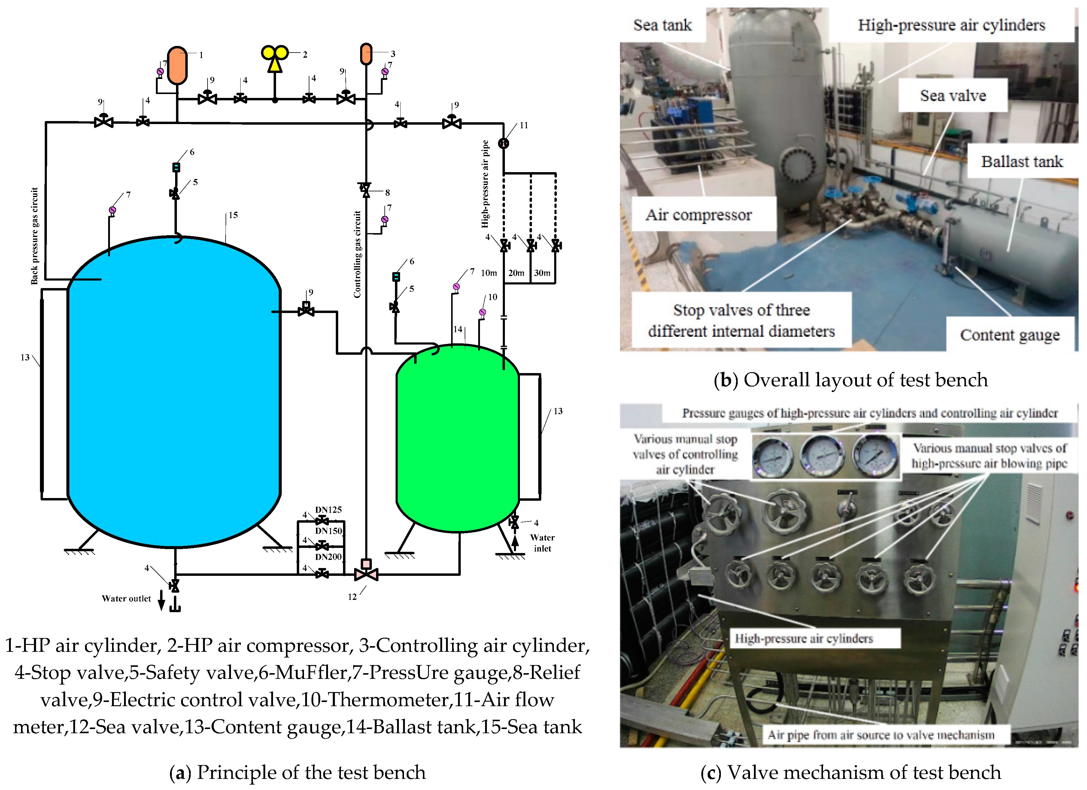
Figure 2.
Typical structure of BPNN.
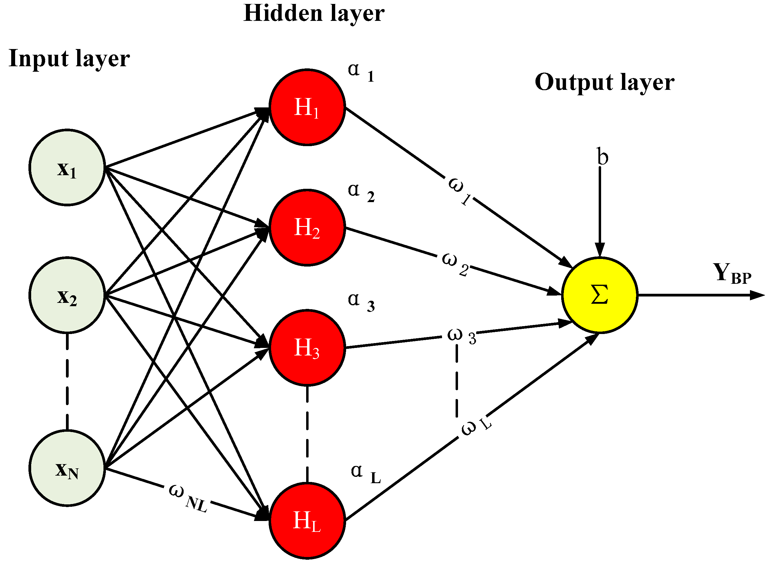
Figure 3.
The proposing algorithm of BPNN.
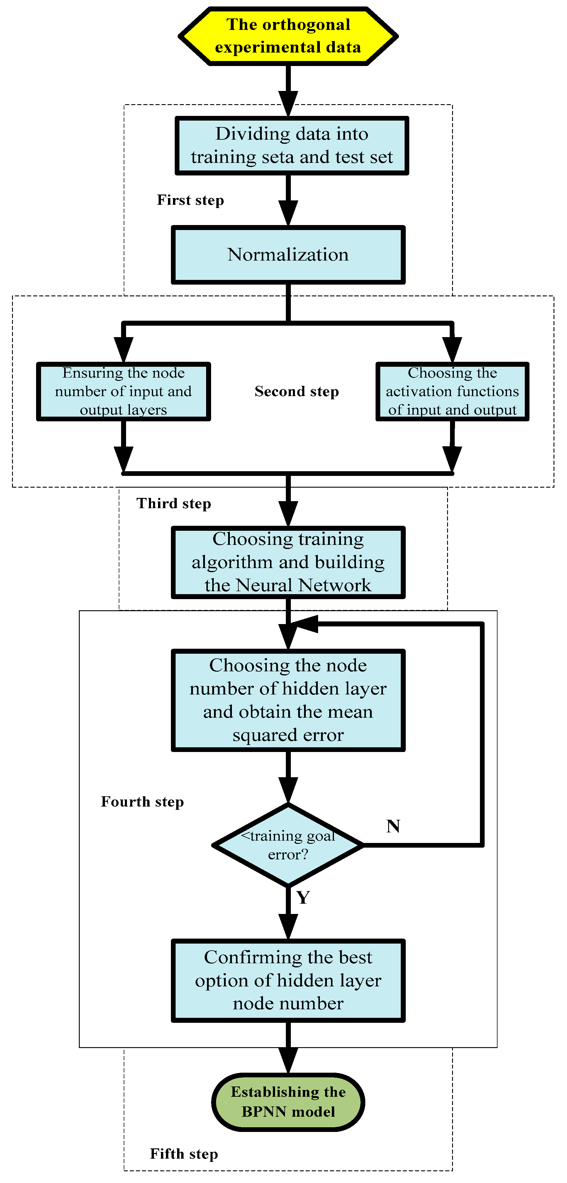
Figure 4.
Evaluation of working-condition1.
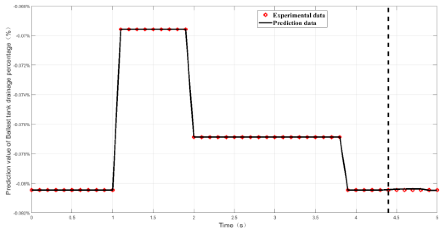
Figure 5.
Evaluation of working-condition2.
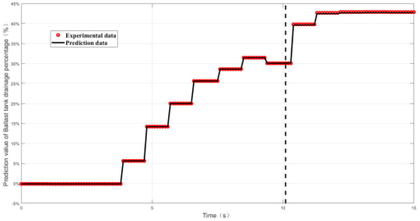
Figure 6.
Evaluation of working-condition3.
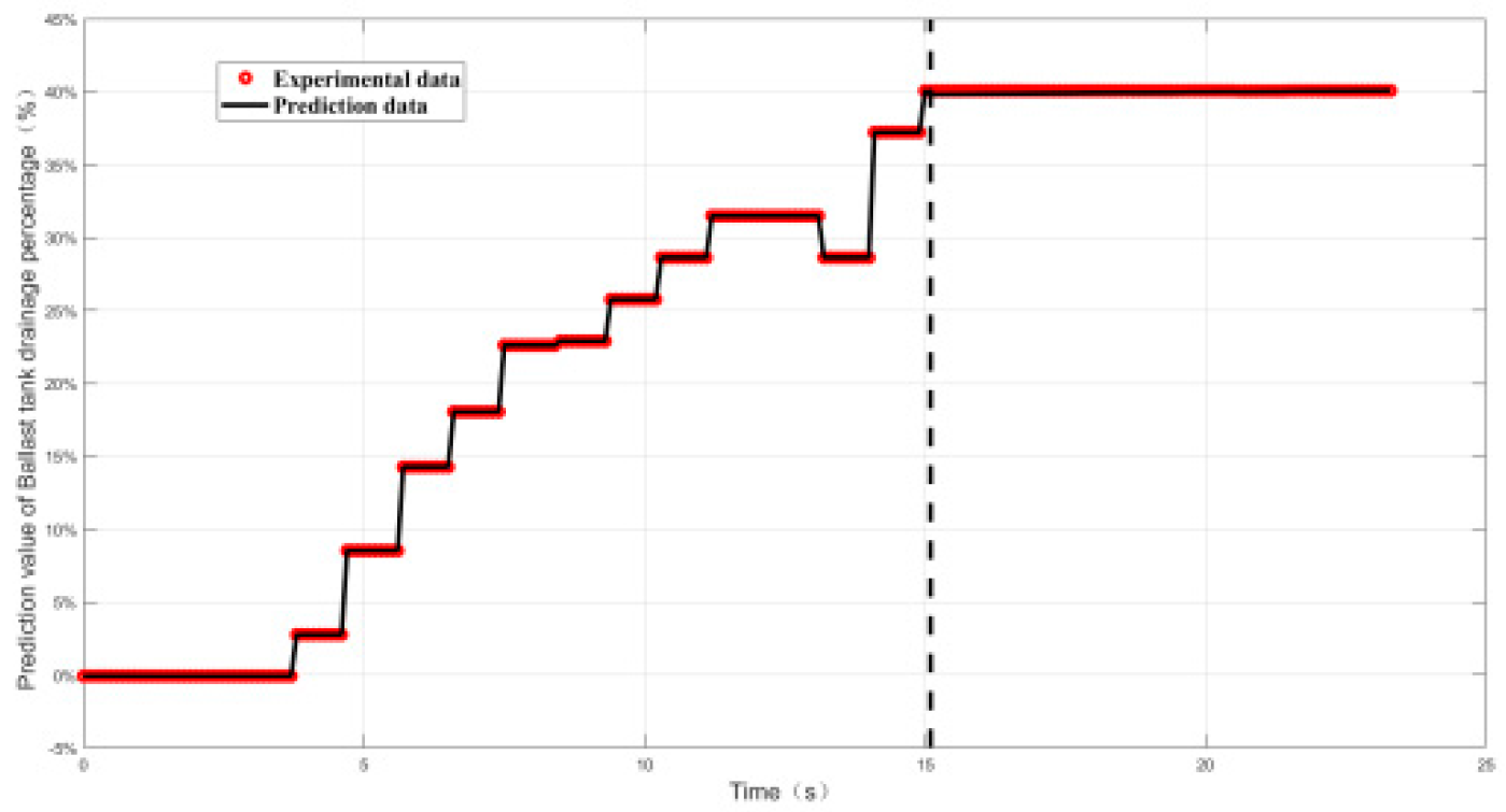
Figure 7.
Evaluation of working-condition4.
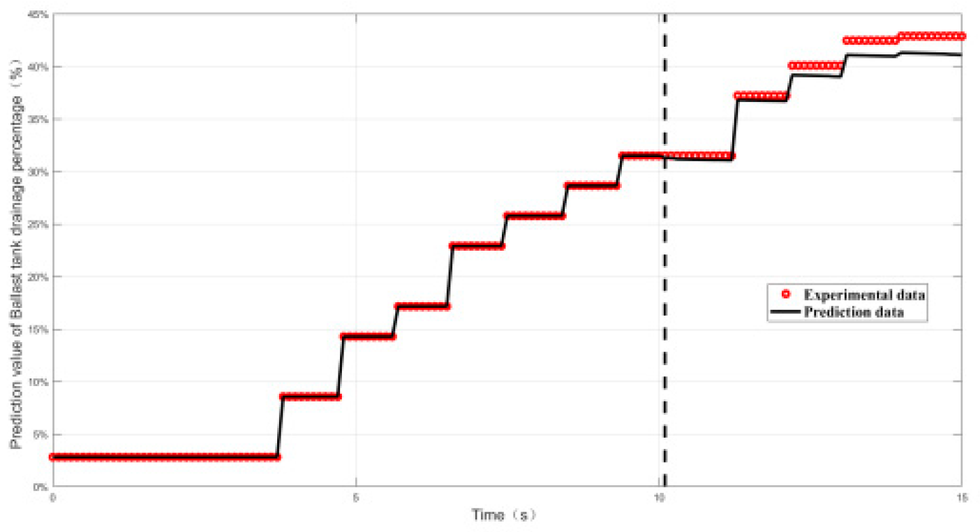
Figure 8.
Evaluation of working-condition3.
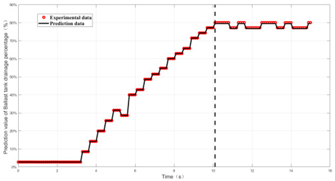
Figure 9.
Evaluation of working-condition4.
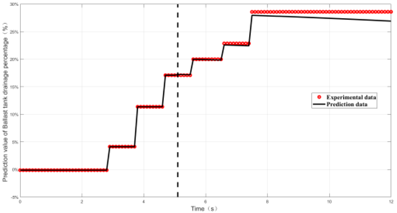
Figure 10.
Evaluation of working-condition7.
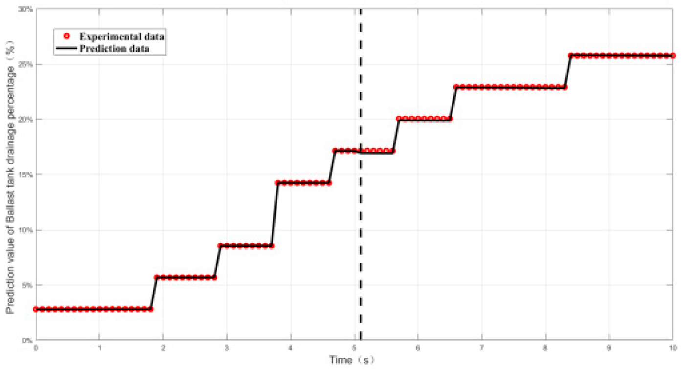
Figure 11.
Evaluation of working-condition8.
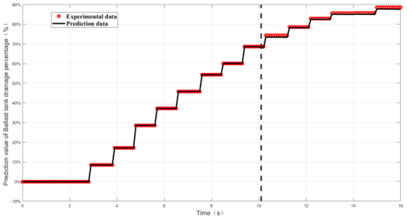
Figure 12.
Evaluation of working-condition9.
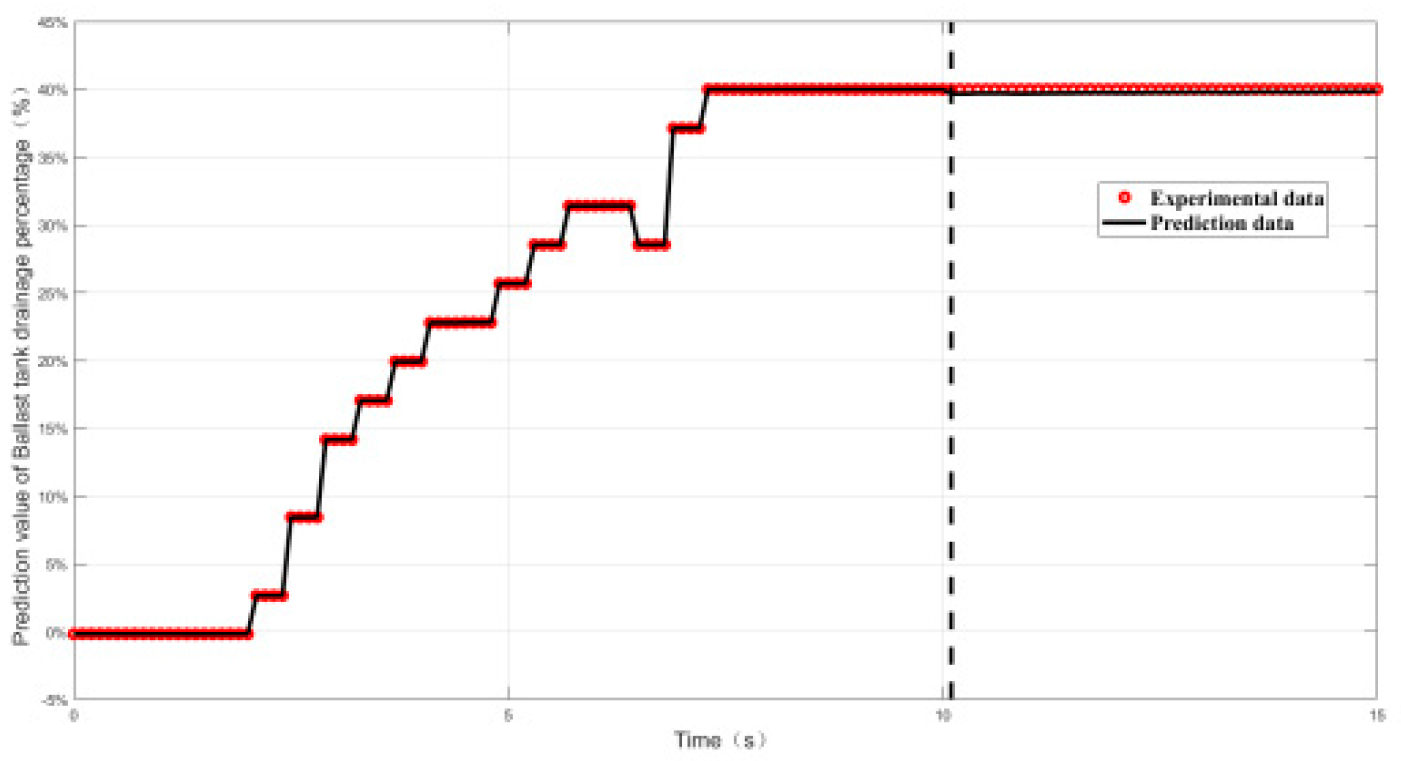
Figure 13.
Evaluation of working-condition10.
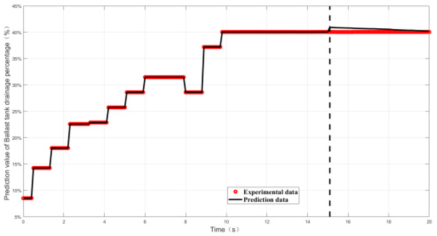
Figure 14.
Evaluation of working-condition11.
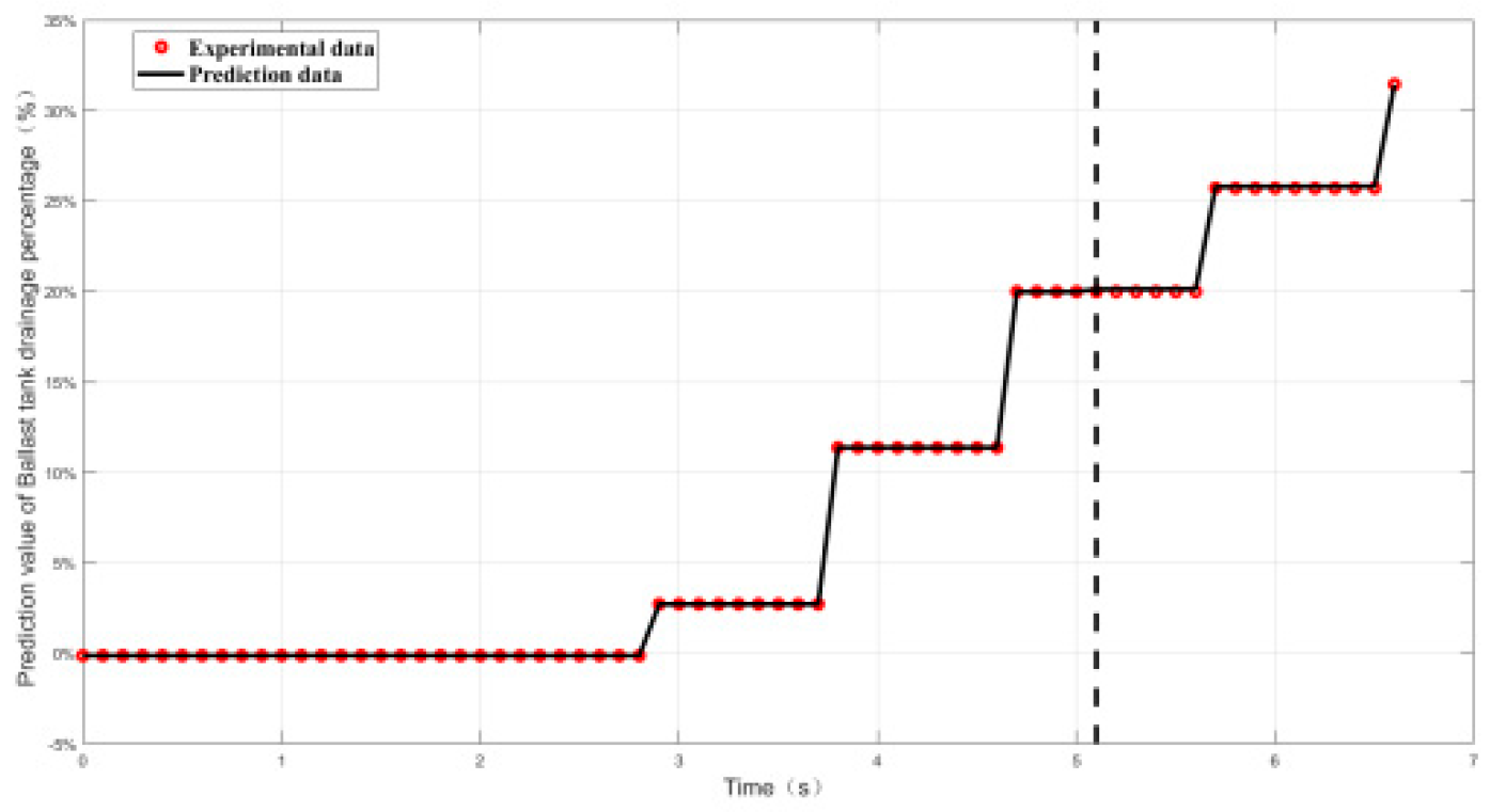
Figure 15.
Evaluation of working-condition12.
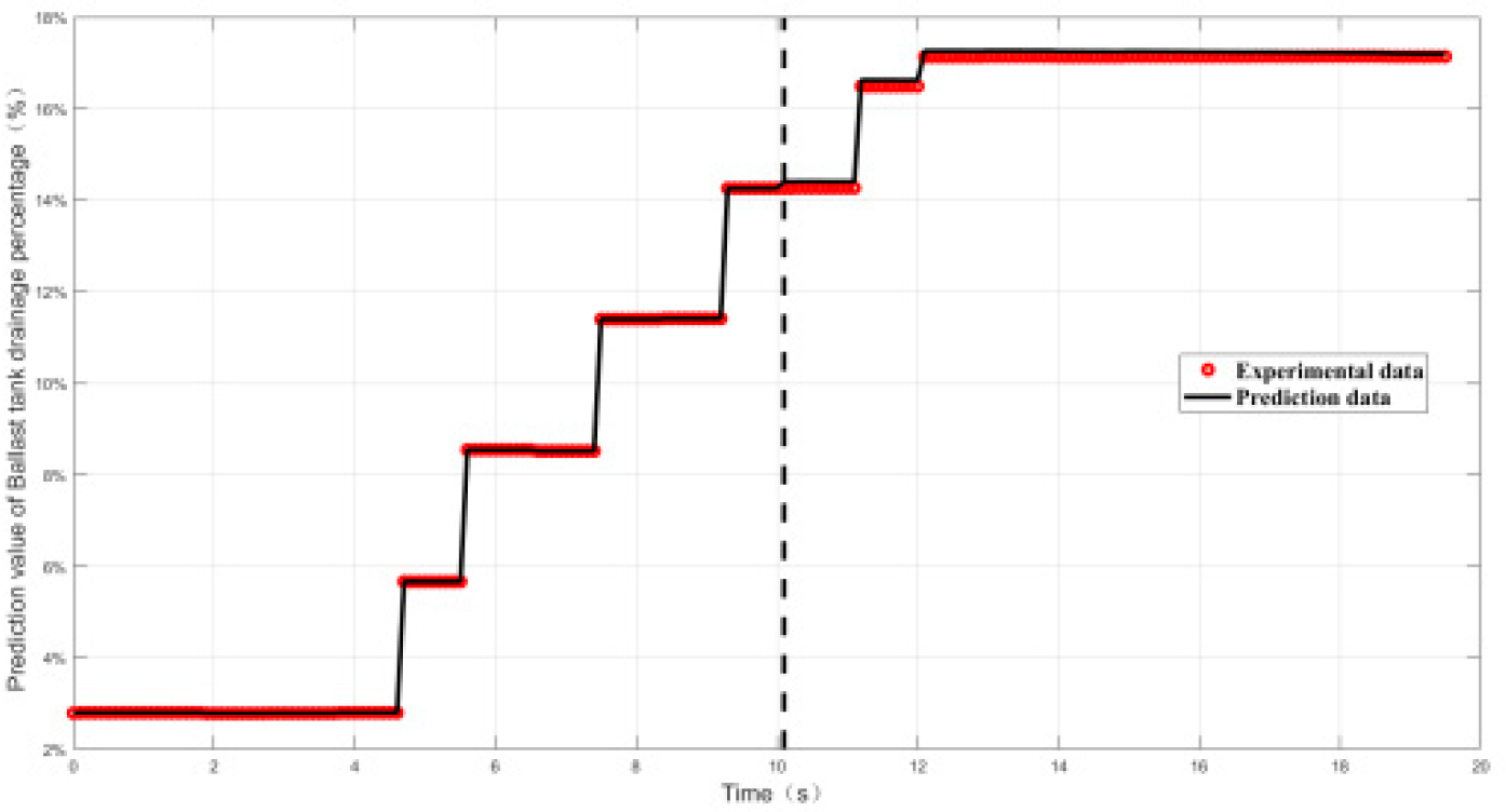
Figure 16.
Evaluation of working-condition13.
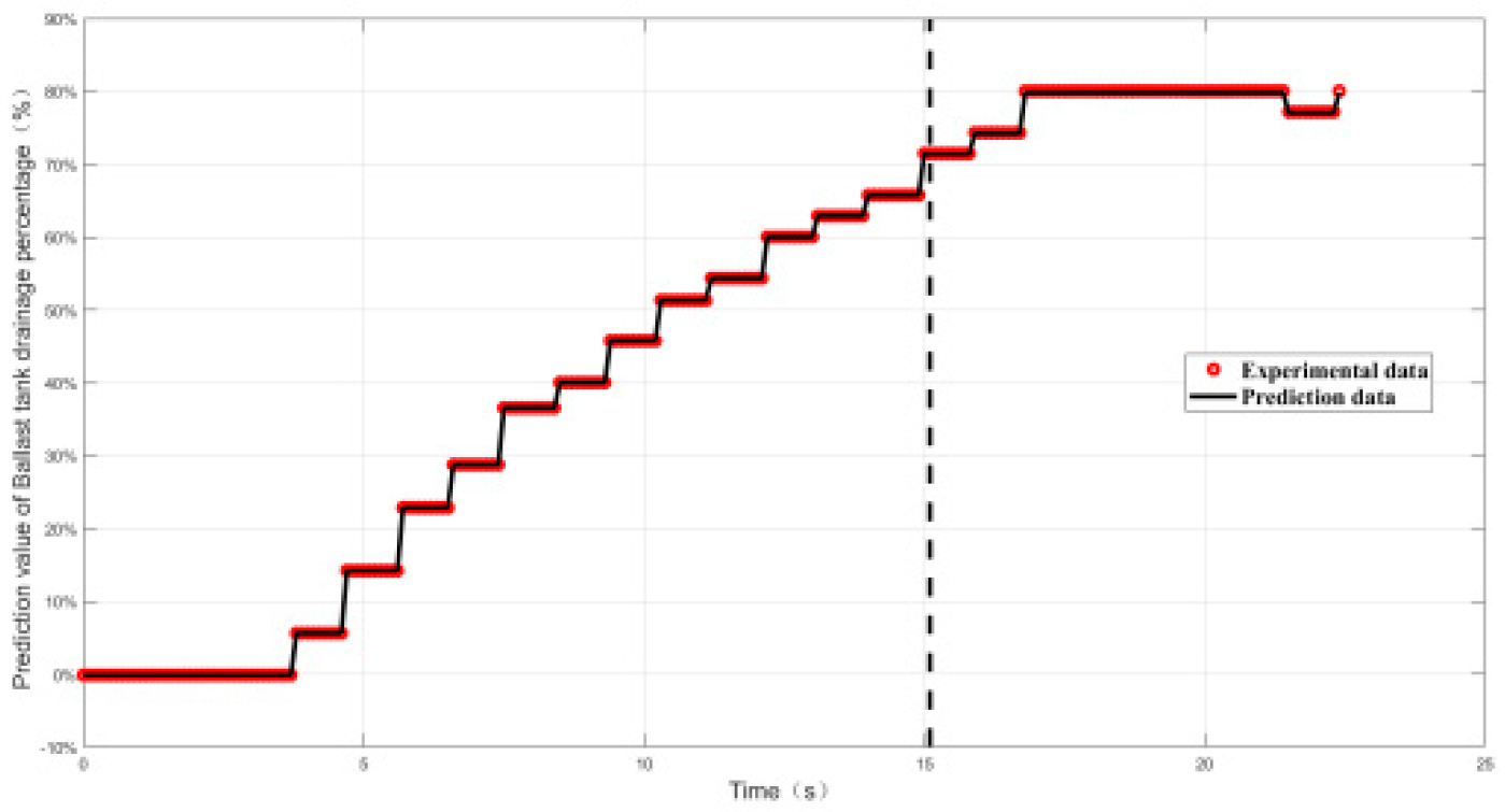
Figure 17.
Evaluation of working-condition14.
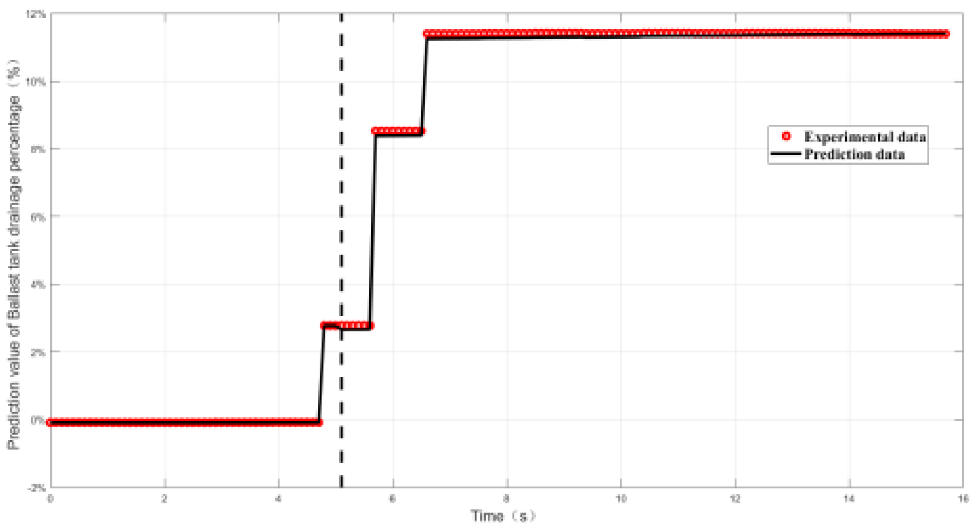
Figure 18.
Evaluation of working-condition13.
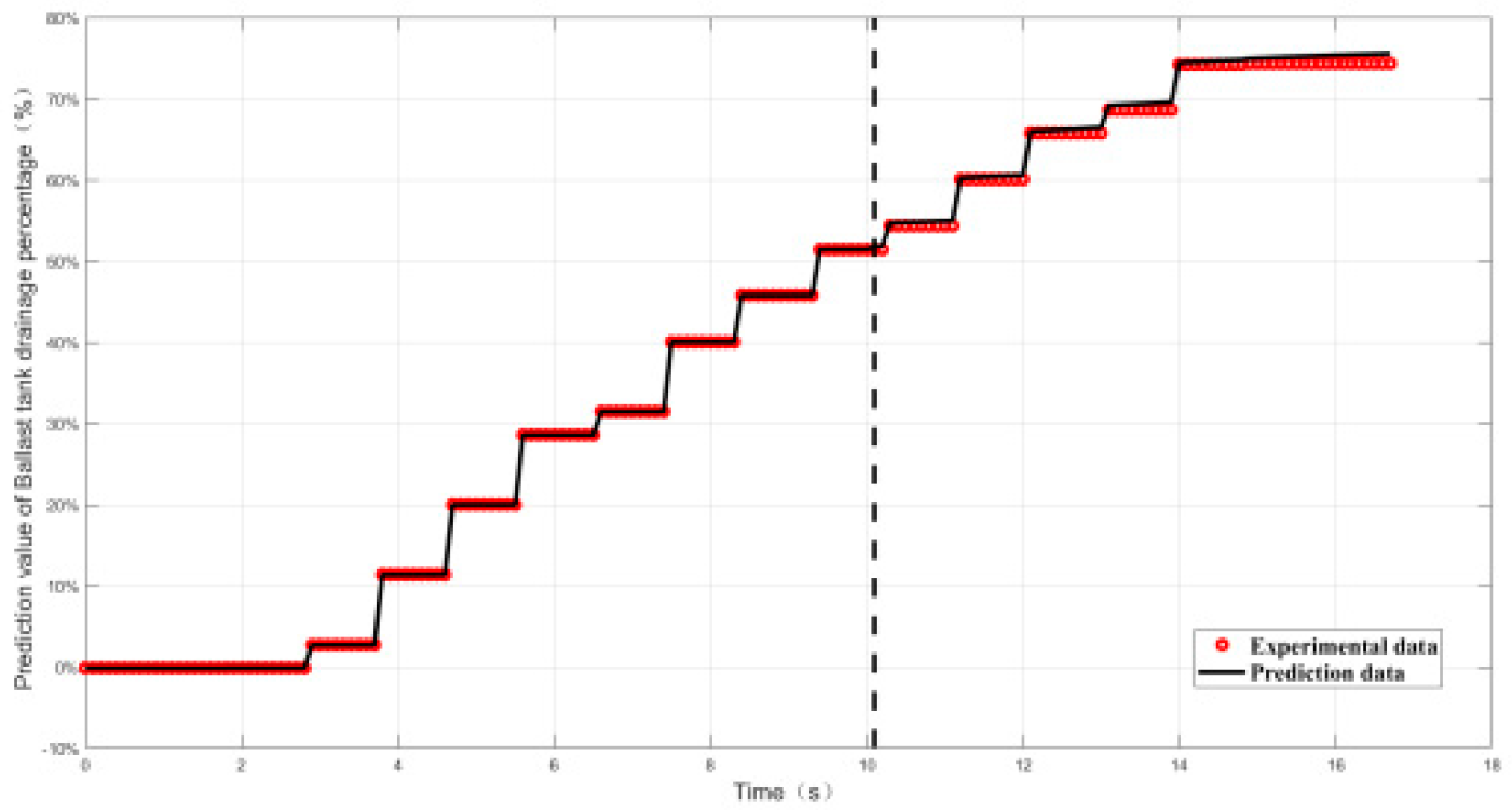
Figure 19.
Evaluation of working-condition16.
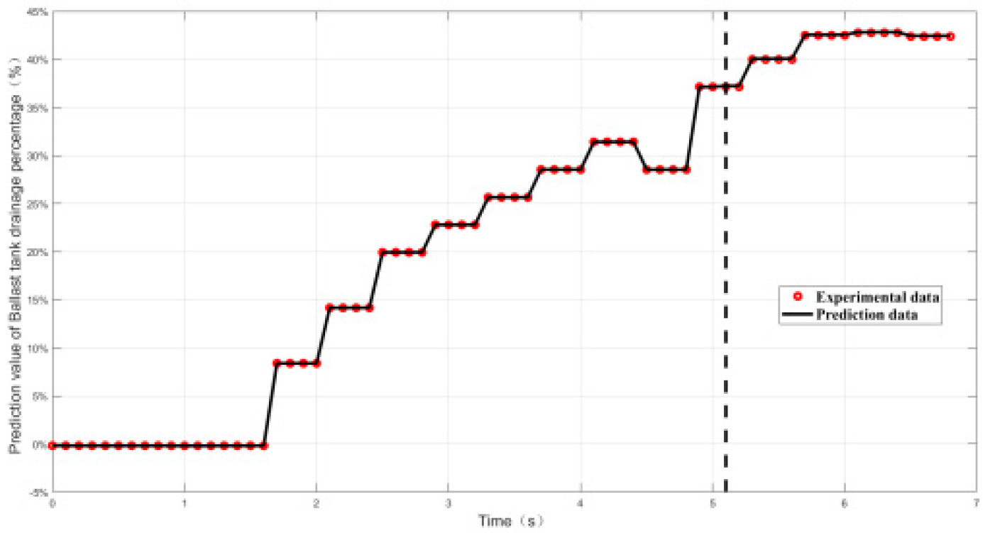
Figure 20.
Evaluation of working-condition17.
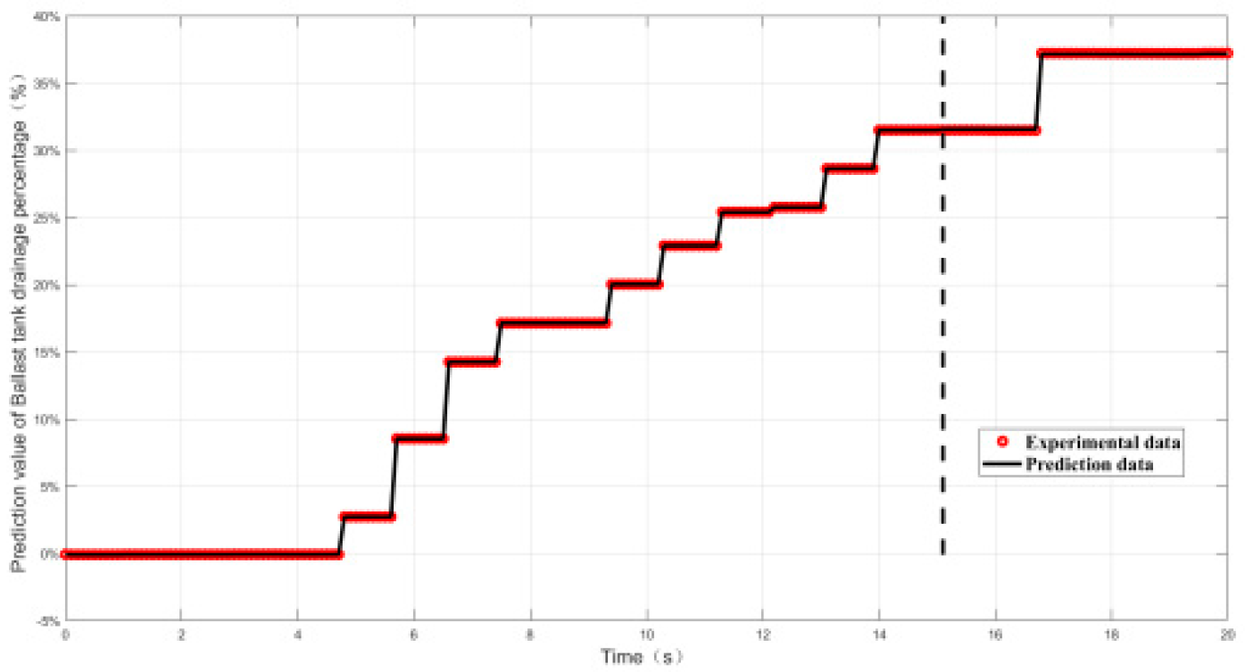
Figure 21.
Evaluation of working-condition18.
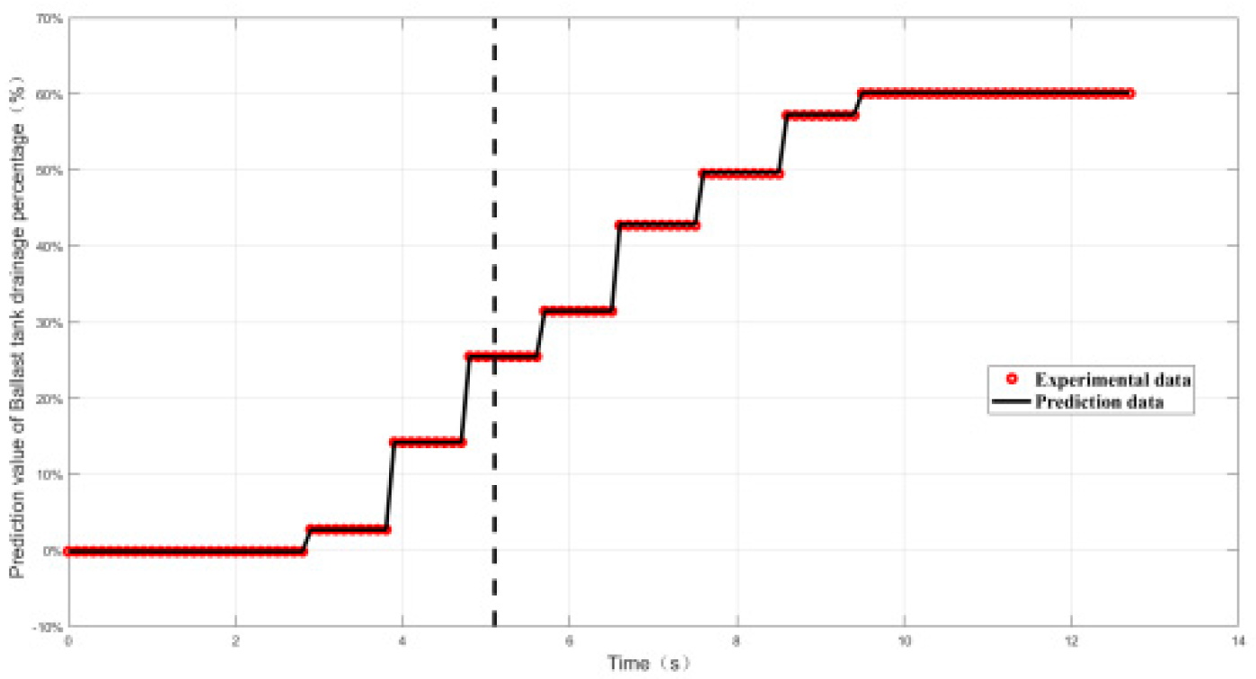
Figure 22.
Prediction Precision percentages of working condition1.
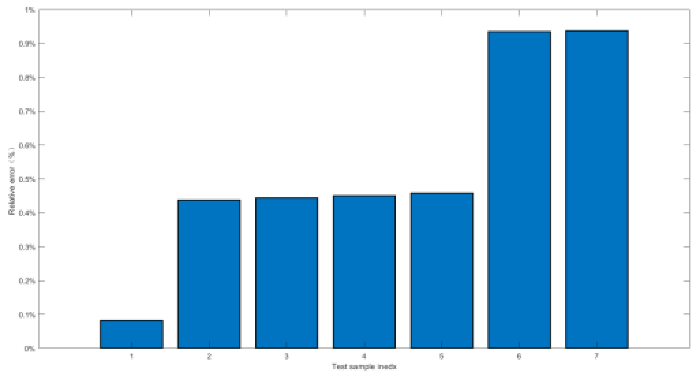
Figure 23.
Prediction Precision percentages of working condition2.
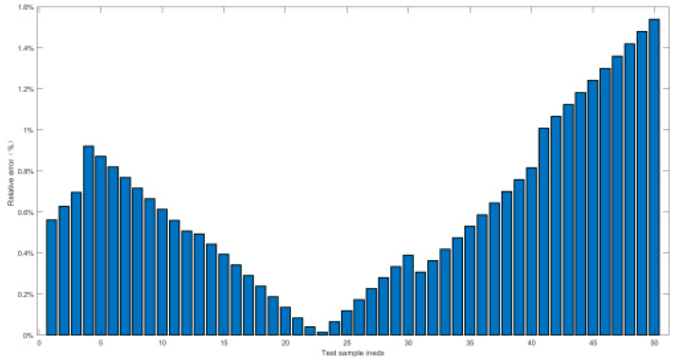
Figure 24.
Prediction Precision percentages of working condition3.
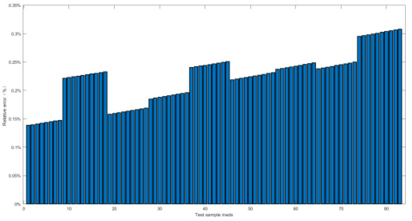
Figure 25.
Prediction Precision percentages of working condition4.
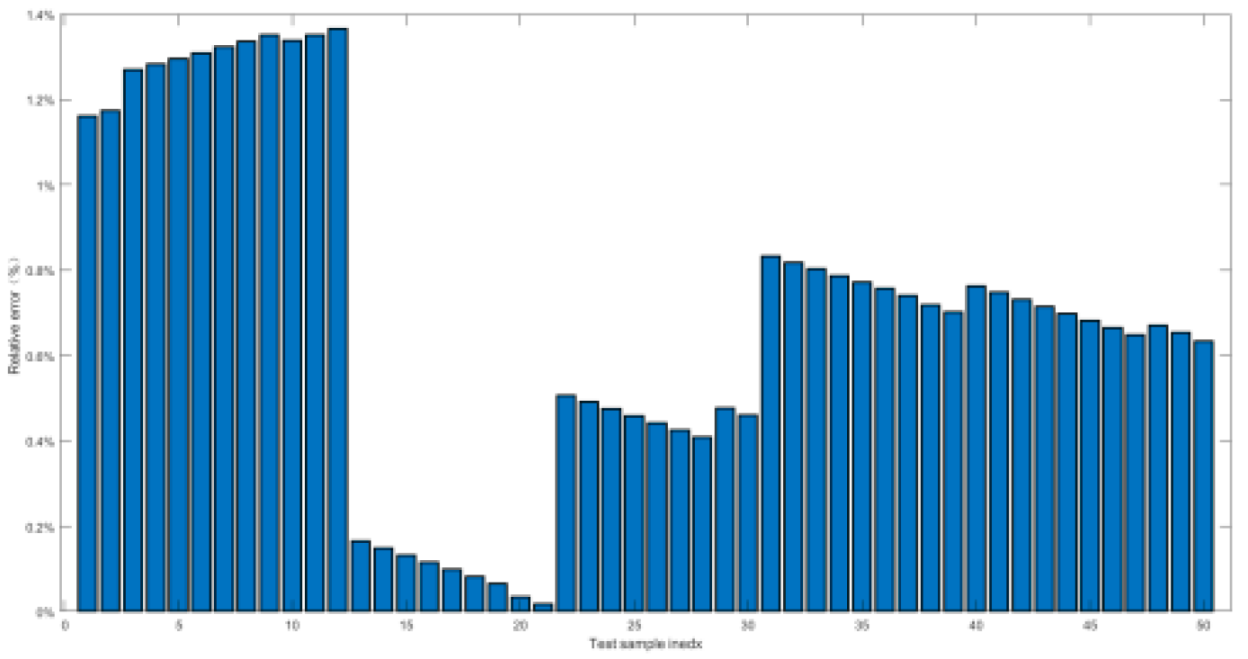
Figure 26.
Prediction Precision percentages of working condition5.
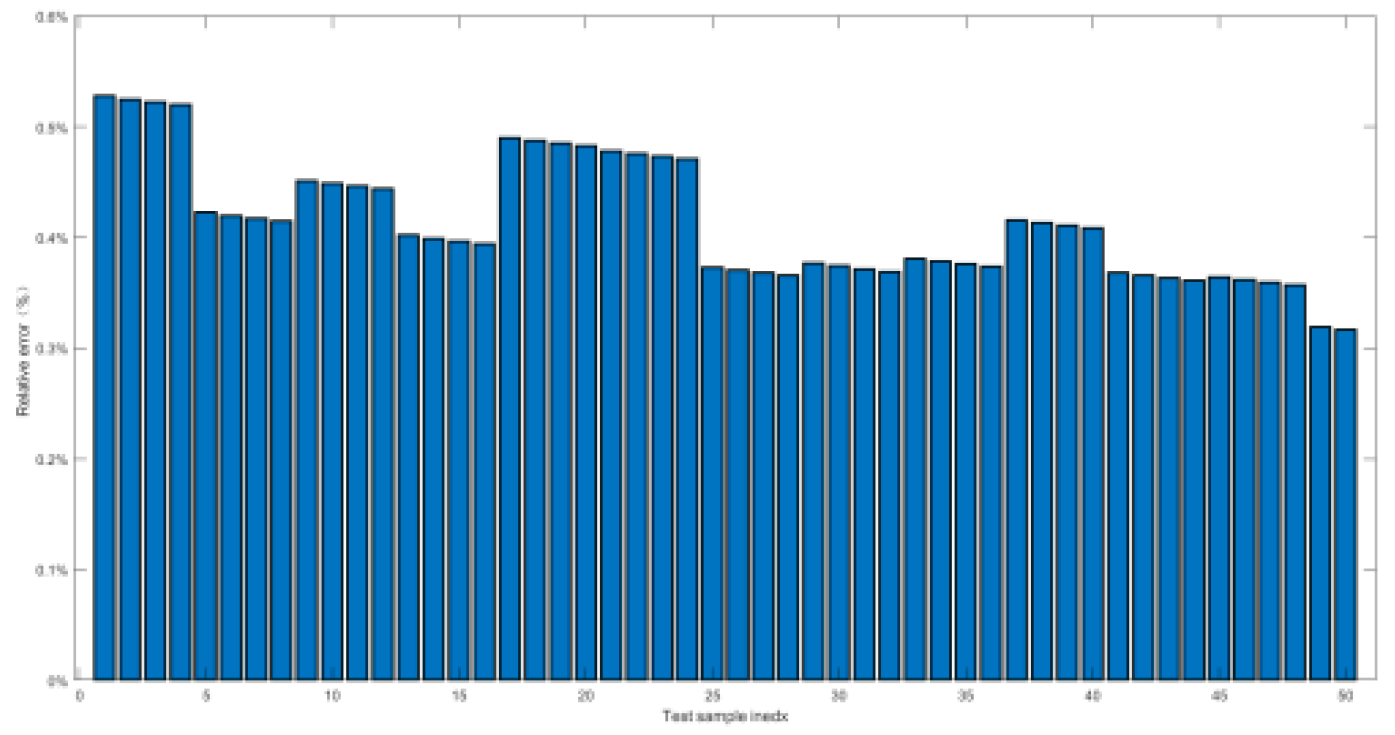
Figure 27.
Prediction Precision percentages of working condition6.
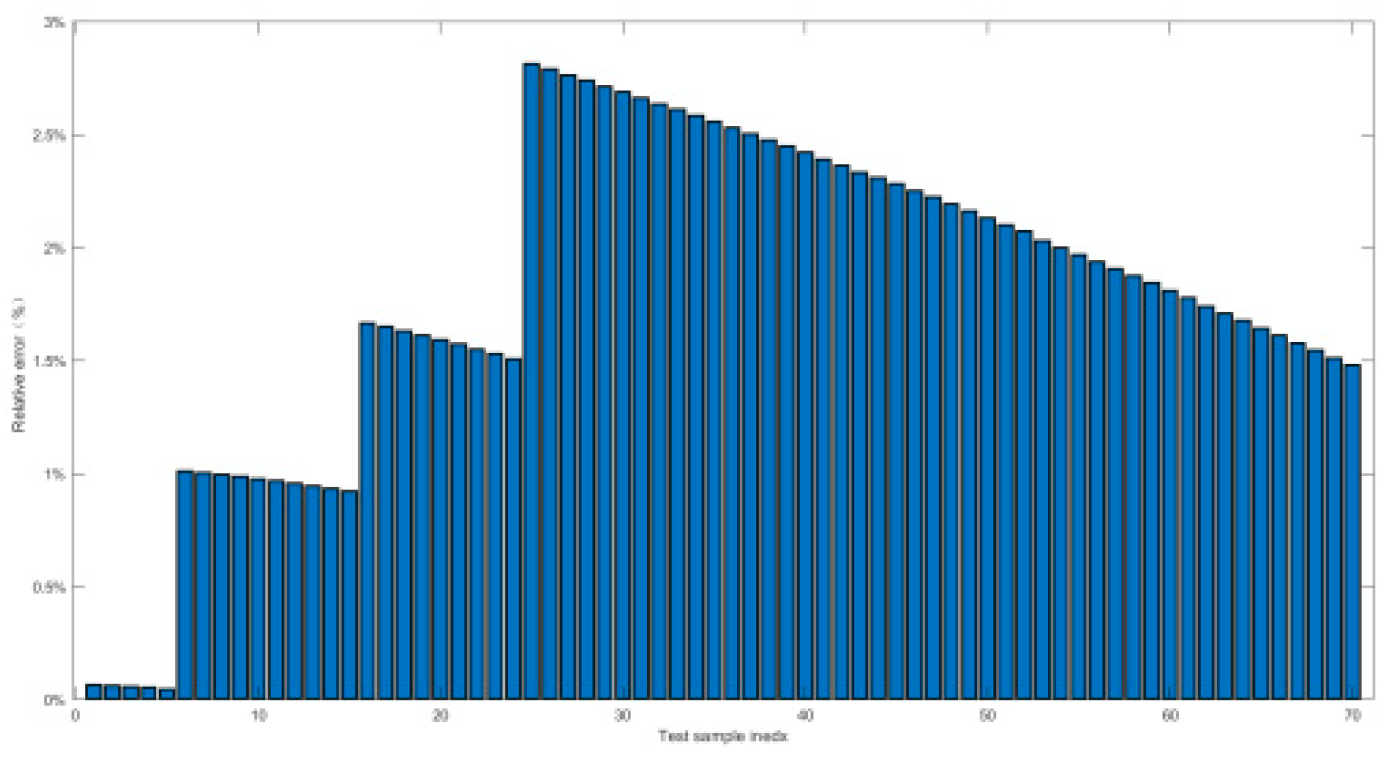
Figure 28.
Prediction Precision percentages of working condition7.
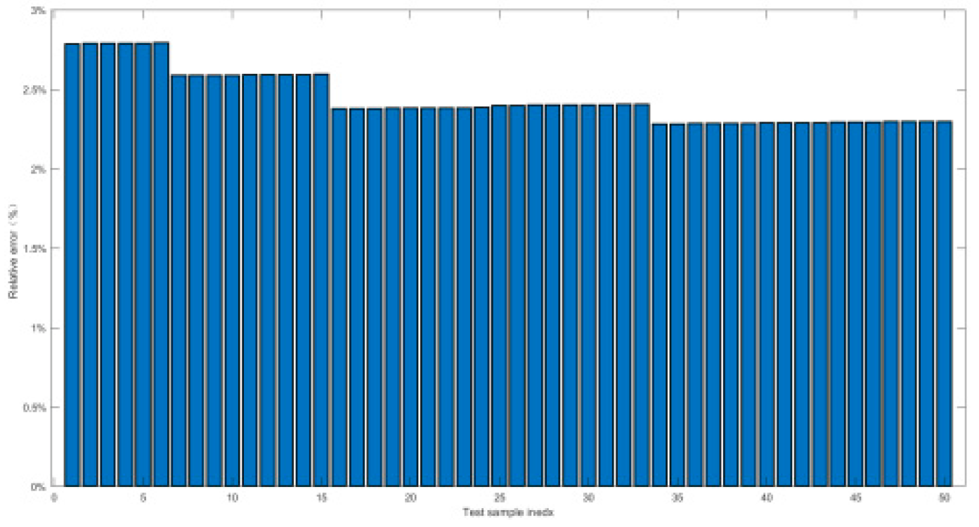
Figure 29.
Prediction Precision percentages of working condition8.
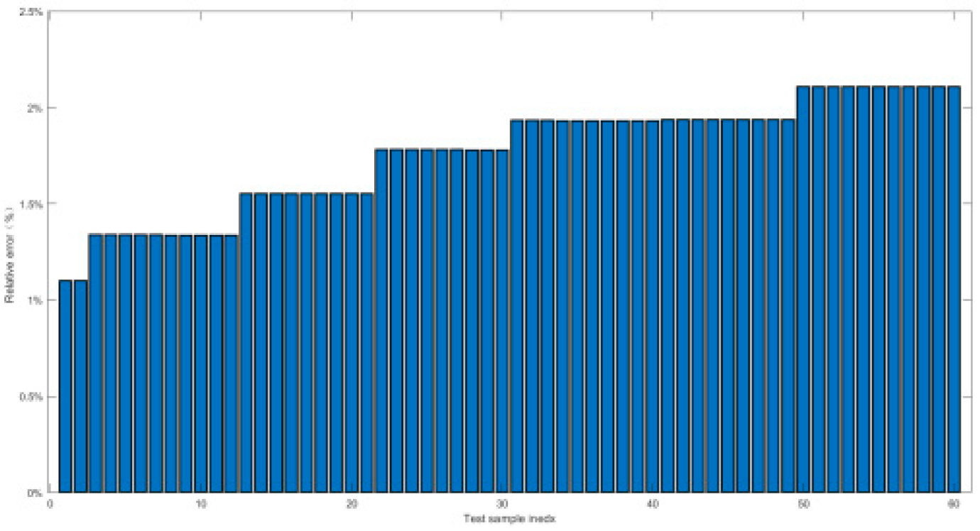
Figure 30.
Prediction Precision percentages of working condition9.
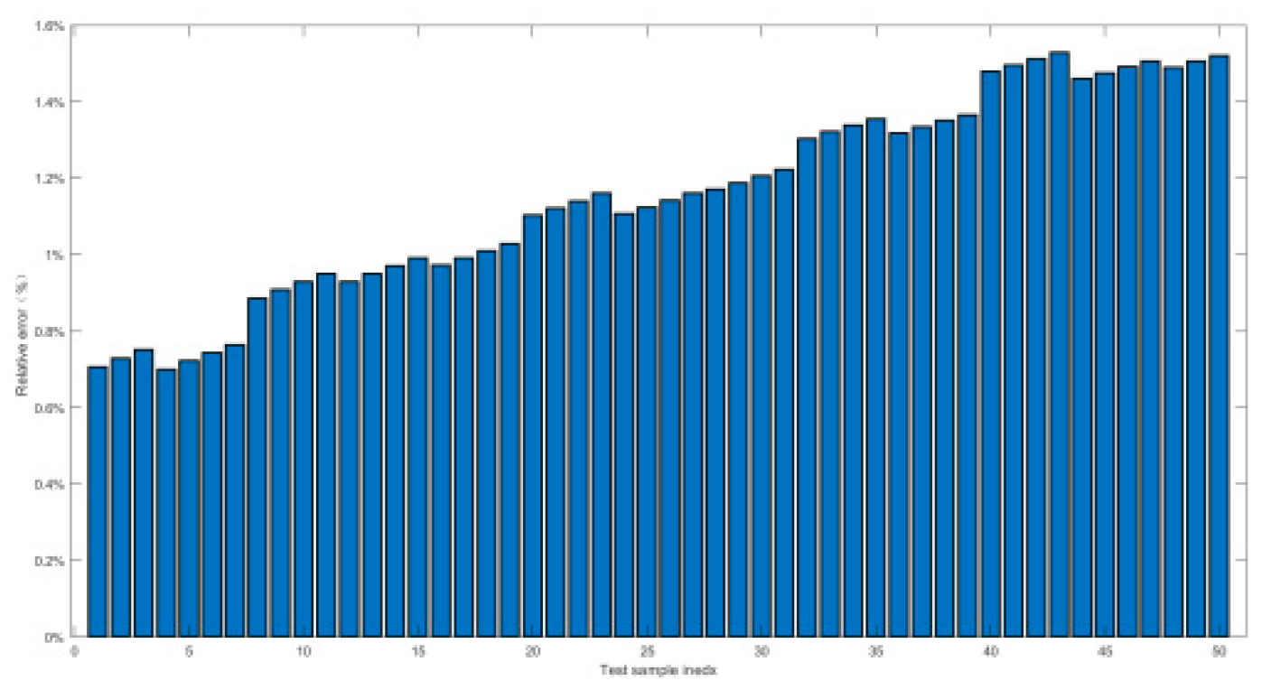
Figure 31.
Prediction Precision percentages of working condition10.
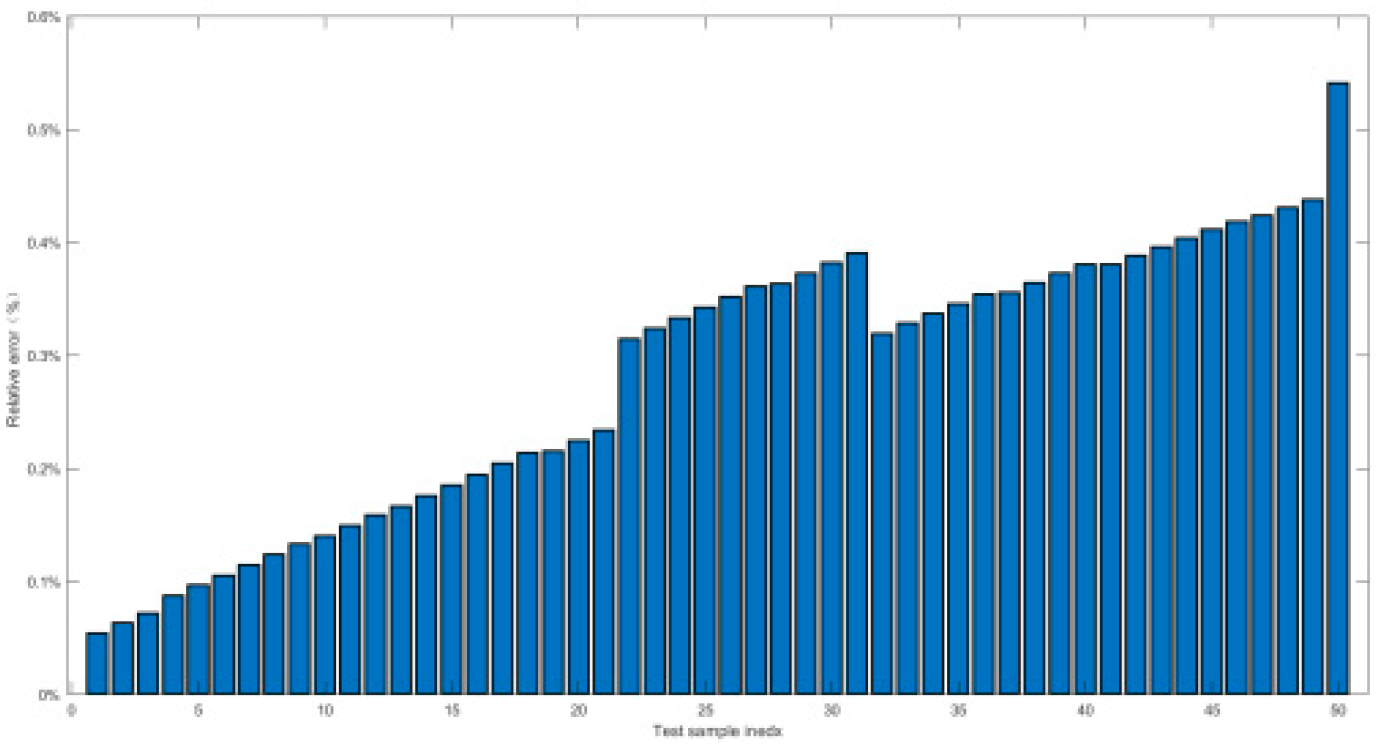
Figure 32.
Prediction Precision percentages of working condition11.
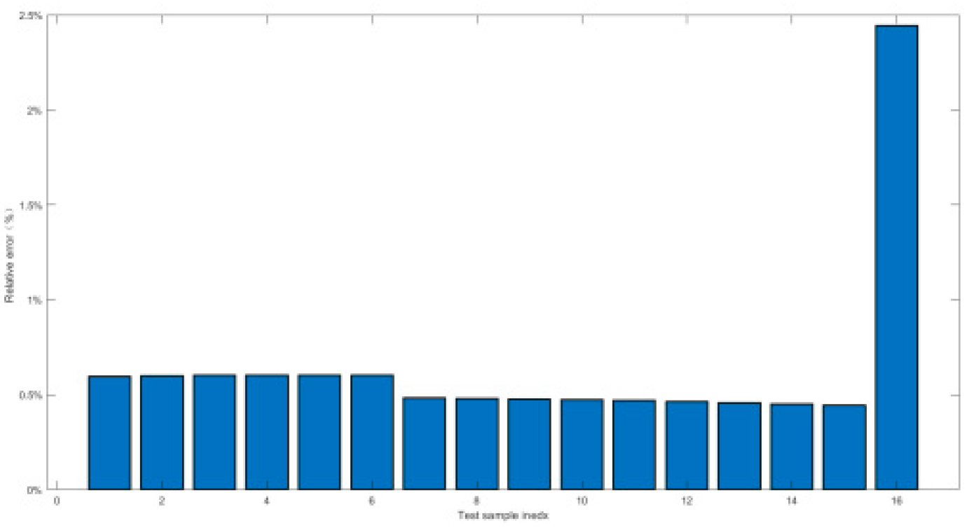
Figure 33.
Prediction Precision percentages of working condition12.
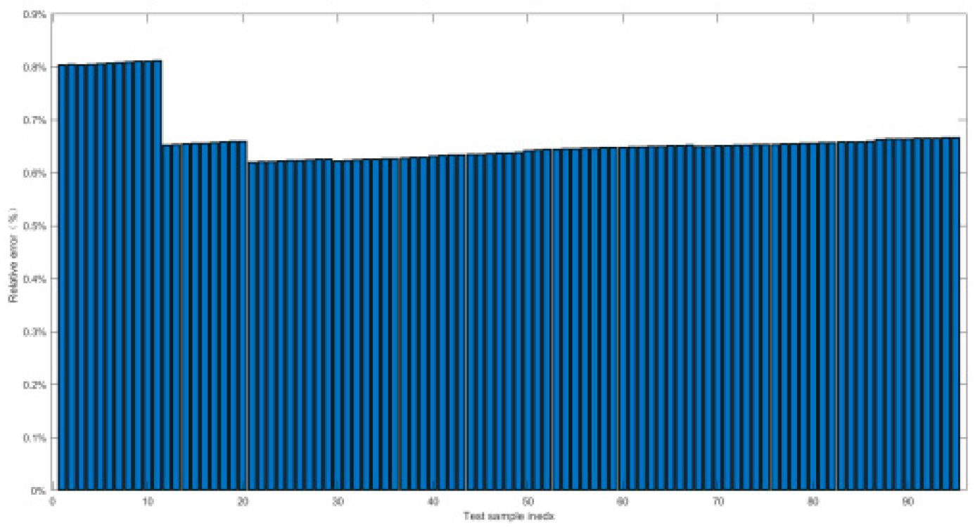
Figure 34.
Prediction Precision percentages of working condition13.
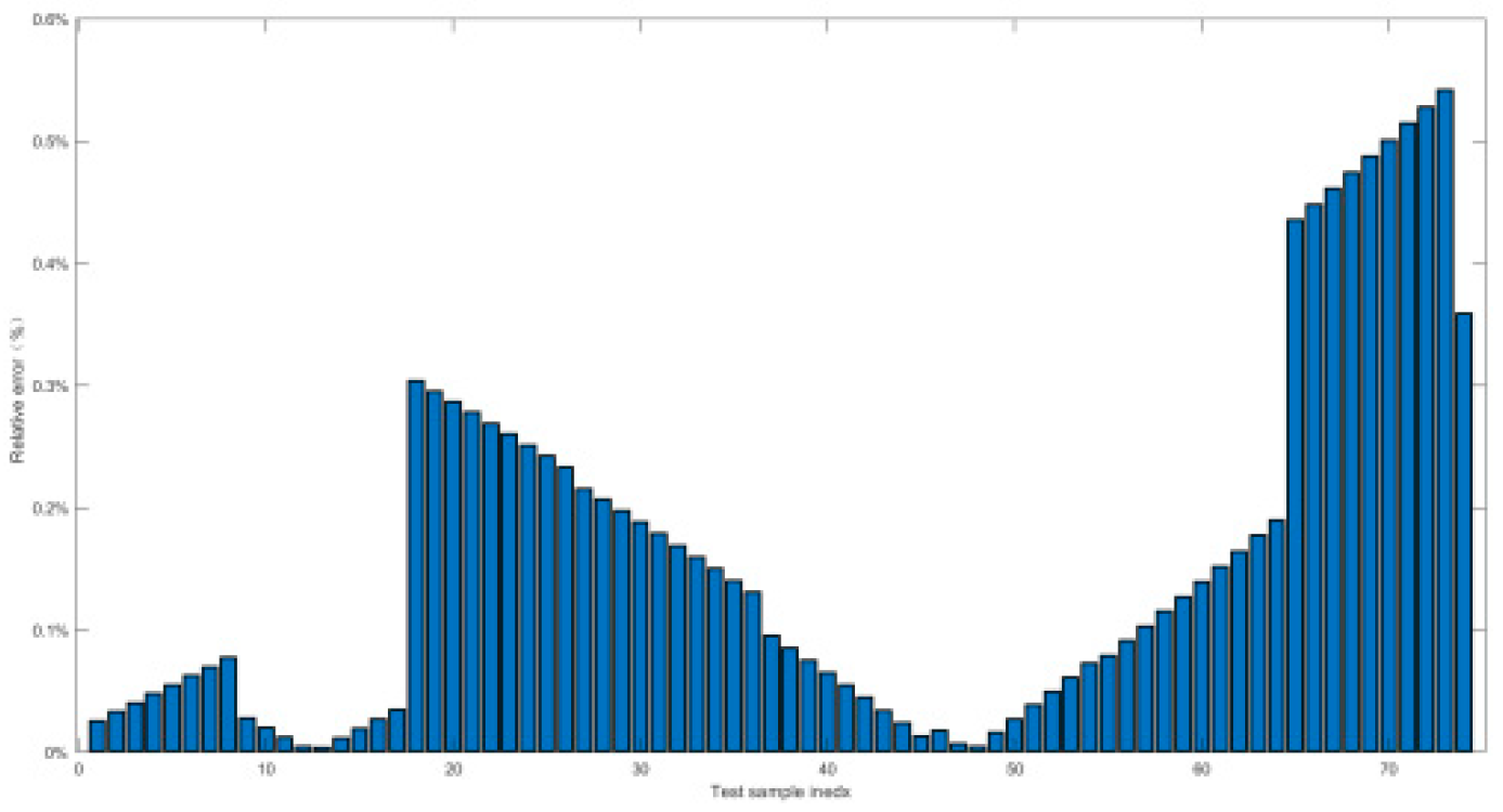
Figure 35.
Prediction Precision percentages of working condition14.
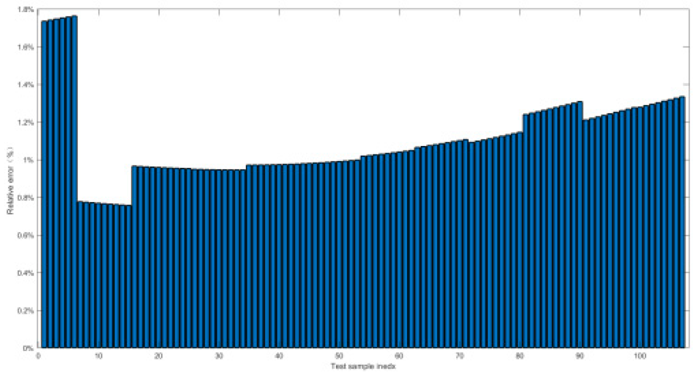
Figure 36.
Prediction Precision percentages of working condition15.
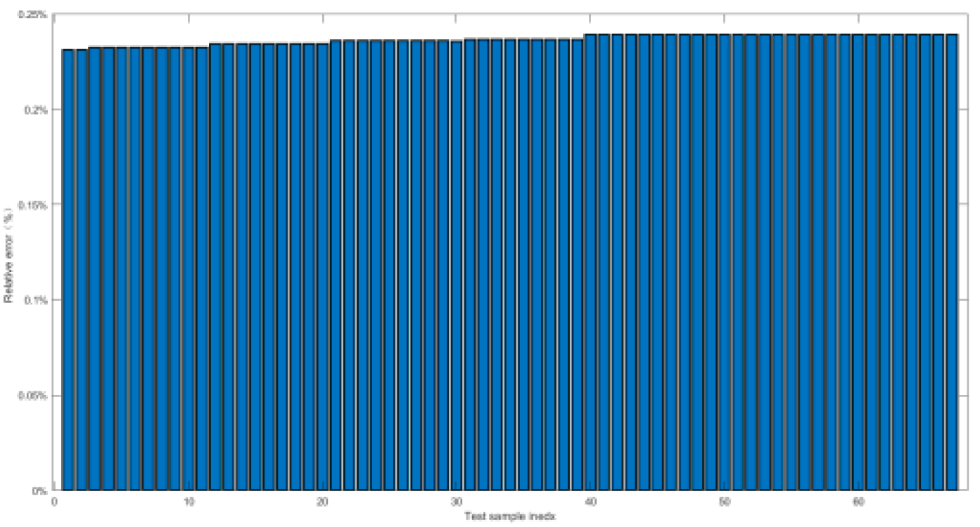
Figure 37.
Prediction Precision percentages of working condition16.
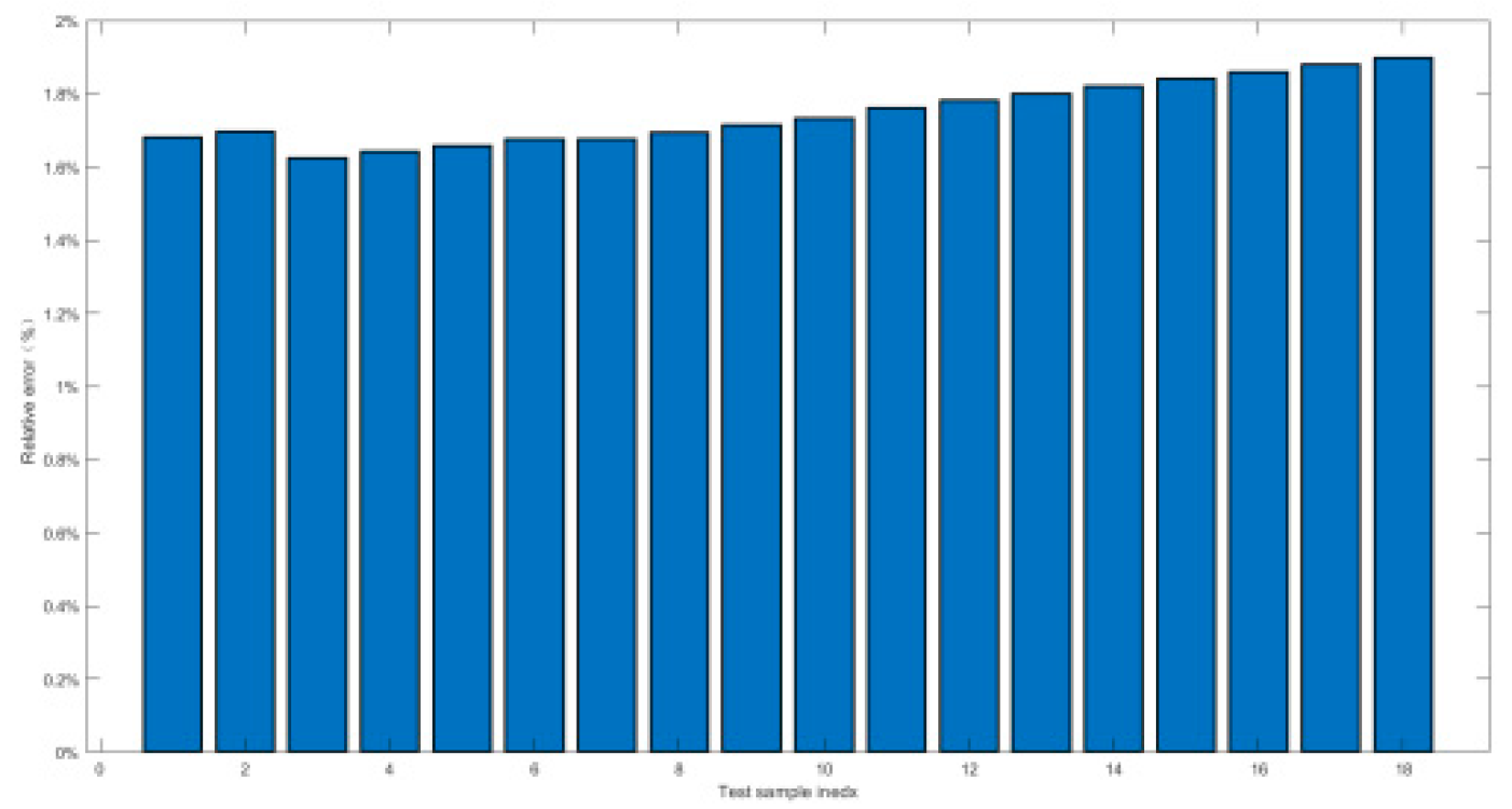
Figure 38.
Prediction Precision percentages of working condition17.
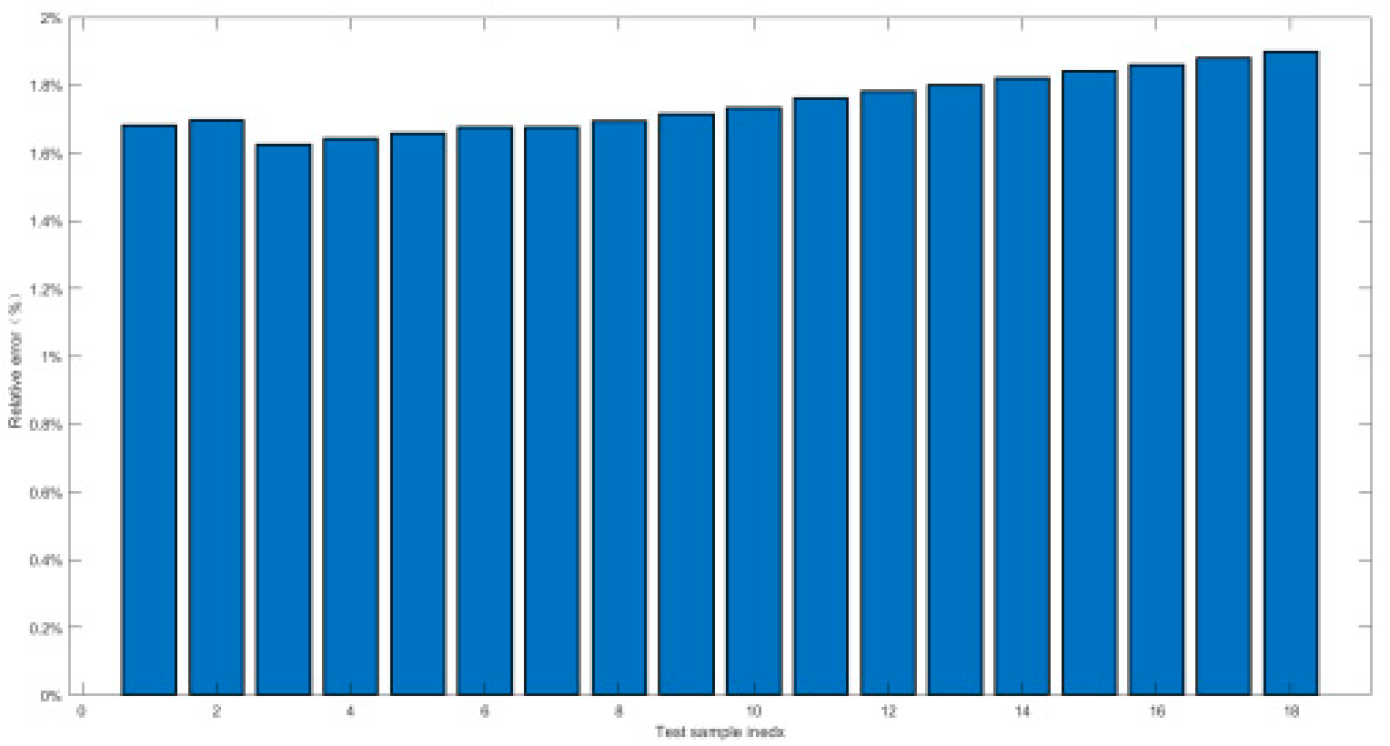
Figure 39.
Prediction Precision percentages of working condition18.
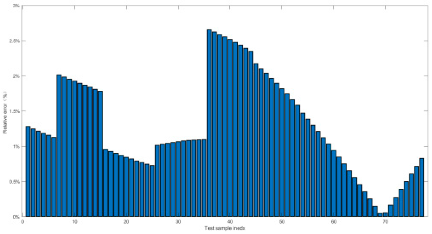
Figure 40.
Pearson analysis heat map.
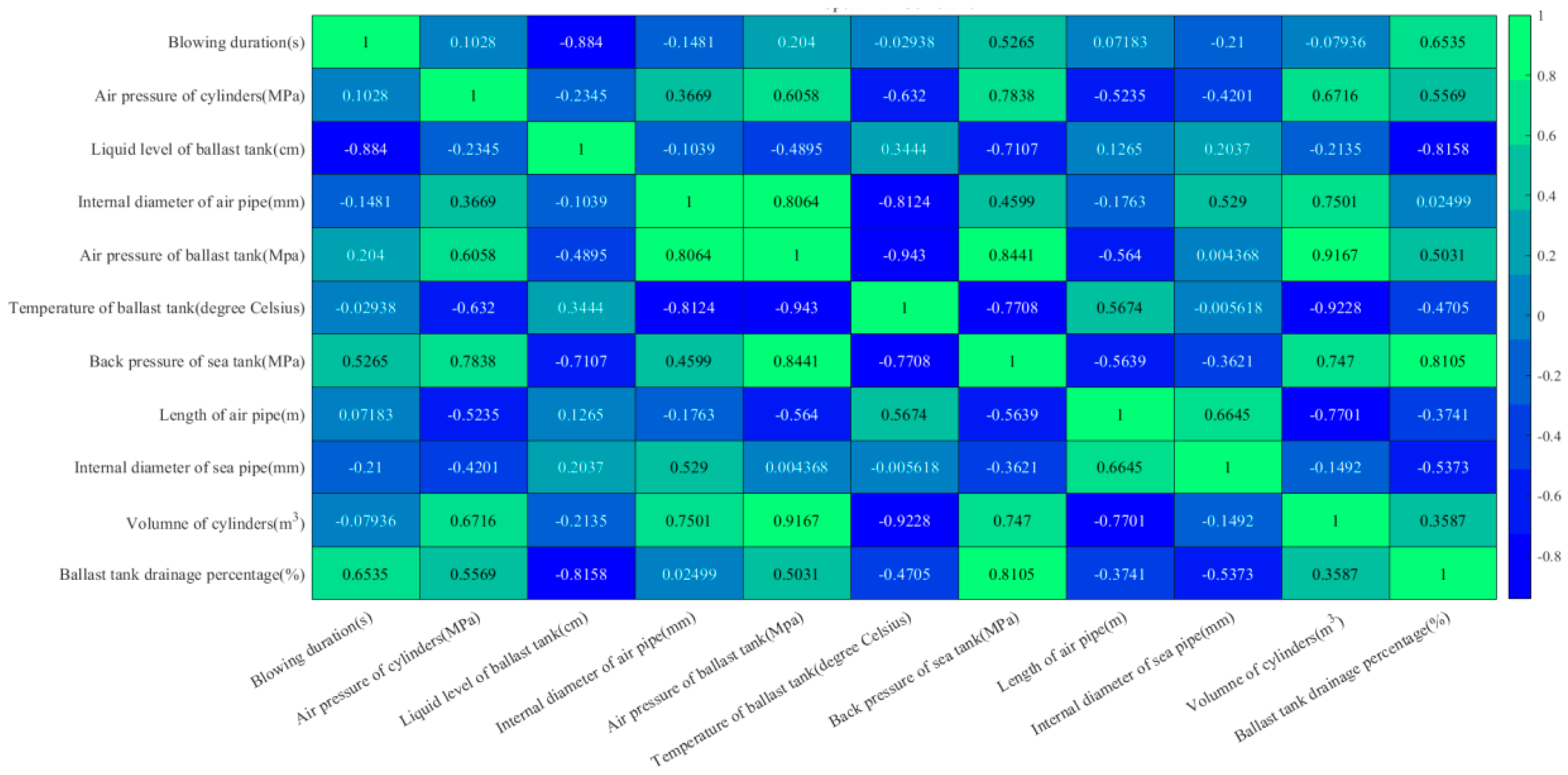
Table 2.
Main parameters of Experimental bench.
| Index | Apparatus | Main Parameters | Remark |
|---|---|---|---|
| 1 | Air compressor | Maximal air inflation pressure is 20.0MPa | |
| 2 | Gas cylinder group | Maximal air working pressure, is 35MPa,volume is 750L | gas source of blowing and back pressure of sea tank |
| 3 | Ballast tank | Volume is 1.2m3 and able to handle pressure of 7MPa | |
| 4 | Sea tank | Volume is 13m3 and able to handle pressure of 5MPa | The back pressure is larger than the maximum working depth of the real ship |
| 5 | Gas supply pipeline | Setting up three kinds of length specifications: 10m, 20m and 30m | Inlet with three replaceable pipe sections of 6mm, 8mm and 10mm internal diameters, 0.3m in length. |
| 6 | Sea pipeline | Setting of 125mm, 150mm and 200mm internal diameters | Connection of ballast tank outlet and sea water tank inlet |
Table 3.
Orthogonal Experiment.
| Index of experiment | Influencing factors | ||||||
|---|---|---|---|---|---|---|---|
| A | B | C | D | E | F | G | |
| 1 | 1 | 1 | 1 | 1 | 1 | 1 | 1 |
| 2 | 1 | 2 | 2 | 2 | 2 | 2 | 2 |
| 3 | 1 | 3 | 3 | 3 | 3 | 3 | 3 |
| 4 | 2 | 1 | 1 | 2 | 2 | 3 | 3 |
| 5 | 2 | 2 | 2 | 3 | 3 | 1 | 1 |
| 6 | 2 | 3 | 3 | 1 | 1 | 2 | 2 |
| 7 | 3 | 1 | 2 | 1 | 3 | 2 | 3 |
| 8 | 3 | 2 | 3 | 2 | 1 | 3 | 1 |
| 9 | 3 | 3 | 1 | 3 | 2 | 1 | 2 |
| 10 | 1 | 1 | 3 | 3 | 2 | 2 | 1 |
| 11 | 1 | 2 | 1 | 1 | 3 | 3 | 2 |
| 12 | 1 | 3 | 2 | 2 | 1 | 1 | 3 |
| 13 | 2 | 1 | 2 | 3 | 1 | 3 | 2 |
| 14 | 2 | 2 | 3 | 1 | 2 | 1 | 3 |
| 15 | 2 | 3 | 1 | 2 | 3 | 2 | 1 |
| 16 | 3 | 1 | 3 | 2 | 3 | 1 | 2 |
| 17 | 3 | 2 | 1 | 3 | 1 | 2 | 3 |
| 18 | 3 | 3 | 2 | 1 | 2 | 3 | 1 |
Table 4.
Extreme variance data table.
| Parameters | A | B | C | D | E | F | G |
|---|---|---|---|---|---|---|---|
| K1 | 213.56% | 263.62% | 197.98% | 105.98% | 226.47% | 189.25% | 329.18% |
| K2 | 243.51% | 225.09% | 224.78% | 227.95% | 213.33% | 230.70% | 216.61% |
| K3 | 217.80% | 260.53% | 252.11% | 340.94% | 235.07% | 254.92% | 129.08% |
| k1 | 35.59% | 43.94% | 33.00% | 17.66% | 37.74% | 31.54% | 54.86% |
| k2 | 40.58% | 37.52% | 37.46% | 37.99% | 35.56% | 38.45% | 36.10% |
| k3 | 36.30% | 43.42% | 42.02% | 56.82% | 39.18% | 42.49% | 21.51% |
| T1 | -1.90% | 6.44% | -4.50% | -19.83% | 0.25% | -5.95% | 17.37% |
| T2 | 3.09% | 0.02% | -0.03% | 0.50% | -1.94% | 0.96% | -1.39% |
| T3 | -1.19% | 5.93% | 4.53% | 19.33% | 1.69% | 4.99% | -15.98% |
| Rx | 4.99% | 6.42% | 9.02% | 39.16% | 3.62% | 10.94% | 33.35% |
| Priority | D>G>F>C>B>A>E | ||||||
| Optimal level | A2 | B1 | C3 | D3 | E3 | F3 | G1 |
| Optimal combination | A2B1C3D3E3F3G1 | ||||||
Table 5.
Variance data table.
| Parameters | A | B | C | D | E | F | G |
|---|---|---|---|---|---|---|---|
| K1 | 213.56% | 263.62% | 197.98% | 105.98% | 226.47% | 189.25% | 329.18% |
| K2 | 243.51% | 225.09% | 224.78% | 227.95% | 213.33% | 230.70% | 216.61% |
| K3 | 217.80% | 260.53% | 252.11% | 340.94% | 235.07% | 254.92% | 129.08% |
| k1 | 35.59% | 43.94% | 33.00% | 17.66% | 37.74% | 31.54% | 54.86% |
| k2 | 40.58% | 37.52% | 37.46% | 37.99% | 35.56% | 38.45% | 36.10% |
| k3 | 36.30% | 43.42% | 42.02% | 56.82% | 39.18% | 42.49% | 21.51% |
| T1 | -1.90% | 6.44% | -4.50% | -19.83% | 0.25% | -5.95% | 17.37% |
| T2 | 3.09% | 0.02% | -0.03% | 0.50% | -1.94% | 0.96% | -1.39% |
| T3 | -1.19% | 5.93% | 4.53% | 19.33% | 1.69% | 4.99% | -15.98% |
| Sx | 0.11% | 1.25% | 0.61% | 11.80% | 0.00% | 1.06% | 9.05% |
| fx | 2 | 2 | 2 | 2 | 2 | 2 | 2 |
| 0.05% | 0.62% | 0.30% | 5.90% | 0.00% | 0.53% | 4.53% | |
| F-ratio | 0.03 | 0.35 | 0.17 | 3.27 | 0.00 | 0.29 | 2.51 |
| Critical value,α=0.05 | 3.24 | 3.24 | 3.24 | 3.24 | 3.24 | 3.24 | 3.24 |
| Effect | insignificant | insignificant | insignificant | significant | insignificant | insignificant | insignificant |
Table 6.
Evaluation indicators of 18 evaluation indicators.
| Index | Evaluation indicators | Data | Remarks |
|---|---|---|---|
| Working condition1 | Sum of Square Errors, ESSE | 1.8906e-12 | Fit between predicted and actual values |
| Mean Absolute Error, EMAE | 4.4939e-7 | Average of the absolute value between the predicted values and actual values | |
| Mean absolute Percentage Error, EMAP | 0.00055853 | Error between datasets of different magnitudes | |
| Mean Square Error, EMSE | 2.7008e-13 | Average of the sum of squares of the prediction errors | |
| Root Mean Square Error, ERMSE | 5.1969e-7 | The square root of the mean of the Square sum of the predicted and actual values | |
| Working condition2 | Sum of Square Errors, ESSE | 0.00012022 | Fit between predicted and actual values |
| Mean Absolute Error, EMAE | 0.001514 | Average of the absolute value between the predicted values and actual values | |
| Mean absolute Percentage Error, EMAP | 0.0036052 | Error between datasets of different magnitudes | |
| Mean Square Error, EMSE | 2.4043e-6 | Average of the sum of squares of the prediction errors | |
| Root Mean Square Error, ERMSE | 0.0015506 | The square root of the mean of the Square sum of the predicted and actual values | |
| Working condition3 | Sum of Square Errors, ESSE | 0.00016132 | Fit between predicted and actual values |
| Mean Absolute Error, EMAE | 0.0011673 | Average of the absolute value between the predicted values and actual values | |
| Mean absolute Percentage Error, EMAP | 0.0029131 | Error between datasets of different magnitudes | |
| Mean Square Error, EMSE | 1.9436e-6 | Average of the sum of squares of the prediction errors | |
| Root Mean Square Error, ERMSE | 0.0013941 | The square root of the mean of the Square sum of the predicted and actual values | |
| Working condition4 | Sum of Square Errors, ESSE | 0.0061557 | Fit between predicted and actual values |
| Mean Absolute Error, EMAE | 0.0096929 | Average of the absolute value between the predicted values and actual values | |
| Mean absolute Percentage Error, EMAP | 0.023948 | Error between datasets of different magnitudes | |
| Mean Square Error, EMSE | 0.00012311 | Average of the sum of squares of the prediction errors | |
| Root Mean Square Error, ERMSE | 0.011096 | The square root of the mean of the Square sum of the predicted and actual values | |
| Working condition5 | Sum of Square Errors, ESSE | 0.001105 | Fit between predicted and actual values |
| Mean Absolute Error, EMAE | 0.0046973 | Average of the absolute value between the predicted values and actual values | |
| Mean absolute Percentage Error, EMAP | 0.0059697 | Error between datasets of different magnitudes | |
| Mean Square Error, EMSE | 2.21e-5 | Average of the sum of squares of the prediction errors | |
| Root Mean Square Error, ERMSE | 0.004701 | The square root of the mean of the Square sum of the predicted and actual values | |
| Working condition6 | Sum of Square Errors, ESSE | 0.0064002 | Fit between predicted and actual values |
| Mean Absolute Error, EMAE | 0.0080078 | Average of the absolute value between the predicted values and actual values | |
| Mean absolute Percentage Error, EMAP | 0.028729 | Error between datasets of different magnitudes | |
| Mean Square Error, EMSE | 9.1432e-5 | Average of the sum of squares of the prediction errors | |
| Root Mean Square Error, ERMSE | 0.009562 | The square root of the mean of the Square sum of the predicted and actual values | |
| Working condition7 | Sum of Square Errors, ESSE | 5.5945e-5 | Fit between predicted and actual values |
| Mean Absolute Error, EMAE | 0.00081209 | Average of the absolute value between the predicted values and actual values | |
| Mean absolute Percentage Error, EMAP | 0.004057 | Error between datasets of different magnitudes | |
| Mean Square Error, EMSE | 1.1189e-6 | Average of the sum of squares of the prediction errors | |
| Root Mean Square Error, ERMSE | 0.0010578 | The square root of the mean of the Square sum of the predicted and actual values | |
| Working condition8 | Sum of Square Errors, ESSE | 0.00635 | Fit between predicted and actual values |
| Mean Absolute Error, EMAE | 0.0095017 | Average of the absolute value between the predicted values and actual values | |
| Mean absolute Percentage Error, EMAP | 0.011281 | Error between datasets of different magnitudes | |
| Mean Square Error, EMSE | 0.00010583 | Average of the sum of squares of the prediction errors | |
| Root Mean Square Error, ERMSE | 0.010288 | The square root of the mean of the Square sum of the predicted and actual values | |
| Working condition9 | Sum of Square Errors, ESSE | 0.00030943 | Fit between predicted and actual values |
| Mean Absolute Error, EMAE | 0.0024449 | Average of the absolute value between the predicted values and actual values | |
| Mean absolute Percentage Error, EMAP | 0.0061119 | Error between datasets of different magnitudes | |
| Mean Square Error, EMSE | 6.1887e-6 | Average of the sum of squares of the prediction errors | |
| Root Mean Square Error, ERMSE | 0.0024877 | The square root of the mean of the Square sum of the predicted and actual values | |
| Working condition10 | Sum of Square Errors, ESSE | 7.5391e-5 | Fit between predicted and actual values |
| Mean Absolute Error, EMAE | 0.0011243 | Average of the absolute value between the predicted values and actual values | |
| Mean absolute Percentage Error, EMAP | 0.0028055 | Error between datasets of different magnitudes | |
| Mean Square Error, EMSE | 1.5078e-6 | Average of the sum of squares of the prediction errors | |
| Root Mean Square Error, ERMSE | 0.0012279 | The square root of the mean of the Square sum of the predicted and actual values | |
| Working condition11 | Sum of Square Errors, ESSE | 8.0629e-5 | Fit between predicted and actual values |
| Mean Absolute Error, EMAE | 0.0016049 | Average of the absolute value between the predicted values and actual values | |
| Mean absolute Percentage Error, EMAP | 0.0064002 | Error between datasets of different magnitudes | |
| Mean Square Error, EMSE | 5.0393e-6 | Average of the sum of squares of the prediction errors | |
| Root Mean Square Error, ERMSE | 0.0022448 | The square root of the mean of the Square sum of the predicted and actual values | |
| Working condition12 | Sum of Square Errors, ESSE | 0.00011633 | Fit between predicted and actual values |
| Mean Absolute Error, EMAE | 0.0011062 | Average of the absolute value between the predicted values and actual values | |
| Mean absolute Percentage Error, EMAP | 0.0066337 | Error between datasets of different magnitudes | |
| Mean Square Error, EMSE | 1.2245e-6 | Average of the sum of squares of the prediction errors | |
| Root Mean Square Error, ERMSE | 0.0011066 | The square root of the mean of the Square sum of the predicted and actual values | |
| Working condition13 | Sum of Square Errors, ESSE | 0.00021467 | Fit between predicted and actual values |
| Mean Absolute Error, EMAE | 0.0012303 | Average of the absolute value between the predicted values and actual values | |
| Mean absolute Percentage Error, EMAP | 0.0015655 | Error between datasets of different magnitudes | |
| Mean Square Error, EMSE | 2.9009e-6 | Average of the sum of squares of the prediction errors | |
| Root Mean Square Error, ERMSE | 0.0017032 | The square root of the mean of the Square sum of the predicted and actual values | |
| Working condition14 | Sum of Square Errors, ESSE | 0.00014928 | Fit between predicted and actual values |
| Mean Absolute Error, EMAE | 0.0011504 | Average of the absolute value between the predicted values and actual values | |
| Mean absolute Percentage Error, EMAP | 0.010992 | Error between datasets of different magnitudes | |
| Mean Square Error, EMSE | 1.3951e-6 | Average of the sum of squares of the prediction errors | |
| Root Mean Square Error, ERMSE | 0.0011812 | The square root of the mean of the Square sum of the predicted and actual values | |
| Working condition15 | Sum of Square Errors, ESSE | 0.00017113 | Fit between predicted and actual values |
| Mean Absolute Error, EMAE | 0.0015861 | Average of the absolute value between the predicted values and actual values | |
| Mean absolute Percentage Error, EMAP | 0.0023651 | Error between datasets of different magnitudes | |
| Mean Square Error, EMSE | 2.5542e-6 | Average of the sum of squares of the prediction errors | |
| Root Mean Square Error, ERMSE | 0.0015982 | The square root of the mean of the Square sum of the predicted and actual values | |
| Working condition16 | Sum of Square Errors, ESSE | 0.00094847 | Fit between predicted and actual values |
| Mean Absolute Error, EMAE | 0.0072352 | Average of the absolute value between the predicted values and actual values | |
| Mean absolute Percentage Error, EMAP | 0.017463 | Error between datasets of different magnitudes | |
| Mean Square Error, EMSE | 5.2693e-5 | Average of the sum of squares of the prediction errors | |
| Root Mean Square Error, ERMSE | 0.007259 | The square root of the mean of the Square sum of the predicted and actual values | |
| Working condition17 | Sum of Square Errors, ESSE | 0.00049875 | Fit between predicted and actual values |
| Mean Absolute Error, EMAE | 0.002734 | Average of the absolute value between the predicted values and actual values | |
| Mean absolute Percentage Error, EMAP | 0.0077481 | Error between datasets of different magnitudes | |
| Mean Square Error, EMSE | 9.975e-6 | Average of the sum of squares of the prediction errors | |
| Root Mean Square Error, ERMSE | 0.0031583 | The square root of the mean of the Square sum of the predicted and actual values | |
| Working condition18 | Sum of Square Errors, ESSE | 0.0043433 | Fit between predicted and actual values |
| Mean Absolute Error, EMAE | 0.0063359 | Average of the absolute value between the predicted values and actual values | |
| Mean absolute Percentage Error, EMAP | 0.012839 | Error between datasets of different magnitudes | |
| Mean Square Error, EMSE | 5.6407e-5 | Average of the sum of squares of the prediction errors | |
| Root Mean Square Error, ERMSE | 0.0075104 | The square root of the mean of the Square sum of the predicted and actual values |
Table 7.
Maximal relative Errors and Precision accuracy of 18 working conditions.
| Index | Maximal value of δ | Prediction accuracy PP% |
|---|---|---|
| Working conditon1 | 0.9% | 100% |
| Working conditon2 | 1.5% | 100% |
| Working conditon3 | 1.5% | 100% |
| Working conditon4 | 1.38% | 100% |
| Working conditon5 | 0.52% | 100% |
| Working conditon6 | 2.7% | 100% |
| Working conditon7 | 2.7% | 100% |
| Working conditon8 | 2% | 100% |
| Working conditon9 | 1.5% | 100% |
| Working conditon10 | 0.55% | 100% |
| Working conditon11 | 2.5% | 100% |
| Working conditon12 | 0.8% | 100% |
| Working conditon13 | 0.55% | 100% |
| Working conditon14 | 1.74% | 100% |
| Working conditon15 | 0.23% | 100% |
| Working conditon16 | 1.8% | 100% |
| Working conditon17 | 1.6% | 100% |
| Working conditon18 | 2.7% | 100% |
Table 8.
Comparison of simulation and experimental results [2].
Table 8.
Comparison of simulation and experimental results [2].
| Index of literature | Relative error | Researching Objects | Remarks |
|---|---|---|---|
| Reference [2] | 0.53%-39.17% | Peak pressure of ballast tank, which was directly related with drainage percentage | None of statistical correlation researches between manipulation factors and blowing |
| Reference [10,11] | 8% | Flowing-rate of high-pressure gas cylinder group, which was closely related with drainage percentage | |
| Reference [8] | <5% | Drainage percentage by gas jet blowing-off, which was a similar method with short-circuit blowing | |
| Reference [9] | <10% | Drainage percentage by gas jet blowing-off, which was a similar method with short-circuit blowing | |
| This paper | 0.23%-2.7% | Drainage percentage of ballast tank during short-circuit blowing |
Disclaimer/Publisher’s Note: The statements, opinions and data contained in all publications are solely those of the individual author(s) and contributor(s) and not of MDPI and/or the editor(s). MDPI and/or the editor(s) disclaim responsibility for any injury to people or property resulting from any ideas, methods, instructions or products referred to in the content. |
© 2024 by the authors. Licensee MDPI, Basel, Switzerland. This article is an open access article distributed under the terms and conditions of the Creative Commons Attribution (CC BY) license (http://creativecommons.org/licenses/by/4.0/).
Copyright: This open access article is published under a Creative Commons CC BY 4.0 license, which permit the free download, distribution, and reuse, provided that the author and preprint are cited in any reuse.


