
Submitted:
24 October 2024
Posted:
25 October 2024
You are already at the latest version
Abstract
Flue gas oxygen content is one of the important parameters in municipal solid waste incineration (MSWI) process. And its stable control is closely related to the incineration efficiency and pollutant emission. The construction of a high-precision and interpretable flue gas oxygen content model is the basis for achieving its optimal control. However, the existing methods have problems such as poor interpretability, low model accuracy, and complex manual hyperparameter adjustment. In view of the above problems, the article proposes a flue gas oxygen content model based on Bayes-ian optimization (BO) main-complement ensemble algorithm. Firstly, the ensemble TS fuzzy re-gression tree (EnTSFRT) is used to construct the main model. Then, the long short term memory network (LSTM) is used to construct the compensation model with the error of the EnTSFRT model as the true value. The weighted value of the main and compensation models is used as the output. Finally, based on the BO algorithm, the hyperparameters of the constructed main-complement ensemble model are optimized to achieve high performance model. Experi-mental results based on real MSWI process data show that the proposed method has good per-formance.
Keywords:
Municipal solid waste incineration (MSWI)
; Flue gas oxygen content
; Main-compensation tree ensemble model
; Ensemble TS fuzzy regression tree (EnTSFRT)
; Long short term memory network (LSTM)
; Bayesian optimization (BO)
1. Introduction
The total amount of municipal solid waste (MSW) in developing countries such as China has grown rapidly with the advancement of urbanization [1], resulting in the phenomenon of “garbage siege” in many cities [2]. To promote the goal of “carbon peak carbon neutralization” [3], the treatment of MSW is urgent. At present, MSW incineration (MSWI) technology has been widely used in the world because of its advantages of harmlessness, reduction and resource utilization [4,5,6]. However, it also emits pollutants. The use of artificial intelligence (AI) technology for pollution reduction research is one of the current hot spots.
In the MSWI process, flue gas oxygen content is one of the key controlled variables that can characterize the incineration efficiency and pollutant emissions [7]. When flue gas oxygen content is too low, the combustion efficiency of MSW will be greatly reduced. And many toxic and harmful gases such as dioxin (DXN) and sulfur dioxide (SO2) will be produced [8]. When flue gas oxygen content is too high, it will increase the emission of combustion NOx gas [8]. Therefore, it is necessary to accurately control flue gas oxygen content. How to construct an effective flue gas oxygen content model is the basis for its accurate control, which is of great significance for the smooth, efficient and environmentally friendly operation of MSWI process.
At present, the modeling of flue gas oxygen content for MSWI process mainly includes mechanism modeling and data-driven modeling [9,10]. Due to the complex mechanism reaction and nonlinear dynamic characteristics, it is difficult to establish an accurate mathematical model of flue gas oxygen content [11]. In the context of AI and information construction, a large amount of industrial data containing mechanism knowledge can be obtained, which makes data-driven modeling methods receive more and more attention [12]. Data-driven modeling is mainly divided into two categories: neural network (NN)-based algorithm [13,14] and tree-based algorithm [15]. The former is weaker than the latter in terms of interpretability. For complex industrial process modeling, there are many reports based on NN modeling. Ma et al. [16] proposed a modeling method of flue gas oxygen content in power plants based on stacked target enhanced autoencoder and long short-term memory (LSTM). Qiao et al. [6] proposed an improved LSTM (ILSTM) modeling method. In the references [17,18,19], a Takagi-Sugeno (TS) fuzzy neural network (TSFNN) controlled object modeling method based on multiple-input multiple output (MIMO) was proposed. Since NN models are composed of many neurons, the connection between neurons is different. With the increase of NN depth and width, the number of parameters increases rapidly, resulting in large memory consumption and resource consumption. Compared with NN, tree models have better generalization and interpretability in terms of small sample modeling. In researches of tree-based modeling, Tang et al. [20] proposed a deep forest regression modeling method based on cross-layer full connection for soft measurement of key process parameters such as product quality and environmental pollution indicators in complex industrial processes. Xia et al. [21] proposed the furnace temperature modeling of MSWI process based on linear regression decision tree (LRDT). However, the MSWI process is complex, and the data has certain uncertainty. And small changes in the input data may lead to completely different tree structures, which makes the model difficult to repeat and explain in some cases, and will reduce the modeling accuracy. Therefore, Xia et al. [22] proposed an ensemble T-S fuzzy regression tree (EnTSFRT) algorithm, introduced fuzzy reasoning [23] to deal with uncertainty, and illustrated the effectiveness of the EnTSFRT model through experiments.
In order to further improve the performance of the model, Yang et al. [24] proposed a dynamic model of a hybrid structure of selective catalytic reduction (SCR) denitrification system. Luo et al. [25] proposed an integrated modeling method that combines the mechanism model with the data-driven model to realize the roller kiln temperature modeling. Dong et al. [26] proposed a hybrid model based on mechanism modeling and data-driven modeling for the construction of leaching system models. The research showed that the compensation model of secondary modeling of the model error can effectively extract the effective information in the error [27]. This main-compensation model mechanism can adopt the same model or different models. For example, gradient boosting decision tree (GBDT) used the same decision tree to construct a multi-level error compensation model [28], and reference [29] adopted NN compensated linear master model. Recenlty, long short term memory network (LSTM) has beed used to model pollutant emission concentration such as NOx and CO in MSWI process with satisfactory performance [30,31]. At present, the main-compensation ensemble controlled object model for flue gas oxygen content has not been reported.
In addition, hyperparameter adjustment based on manual approach is complex and time-consuming in the modeling process, and it is easy to fall into local optimum. To solve this problem, Ma et al. [32] proposed the particle swarm optimization algorithm to optimize the multi-task NN model. Zhou et al. [33] proposed Bayesian optimization (BO)-based online robust parameter selection for sequential support vector regression. Deng et al. [34] used the improved sparrow search algorithm to optimize the squeeze casting process parameters intelligently.
In summary, the article proposes the BO-EnTSFRT-LSTM algorithm. The algorithm takes primary air volume, secondary air volume, feeder speed average, drying grate speed average and ammonia injection amount as the manipulated variables (MVs). At the same time, considering that there are many hyperparameters in the main-compensation ensemble model, BO is proposed to optimize the hyperparameters. Firstly, the main model is constructed based on EnTSFRT. Secondly, the error of the EnTSFRT model is taken as the true value to construct the LSTM-based model. Finally, BO is used to optimize the hyperparameters.
The innovation of the article is reflected in: (1) The main modeling based on tree algorithm is proposed to improve the interpretability of the controlled object model. (2) A method of hyperparameters selection of the main-complement ensemble model based on BO algorithm is proposed. It reduces the complexity and time-consuming of manual hyperparameter adjustment approach and enhances the model performance. (3) A main-complement ensemble model based on BO optimization for flue gas oxygen content is constructed for the first time. It provides support for related intelligent control research.
The rest of the organizational structure of this article is arranged as follows. Section Ⅱ describes the MSWI process for flue gas oxygen content , the overall modeling strategy and the implementation of the algorithm. In section Ⅲ, the experimental research is carried out, and the experimental results are analyzed to verify the feasibility and superiority of the proposed method. Section Ⅳ summarizes and proposes future research directions.
2. Materials and Methods
2.1. MSWI Process Description for Key Controlled Variables
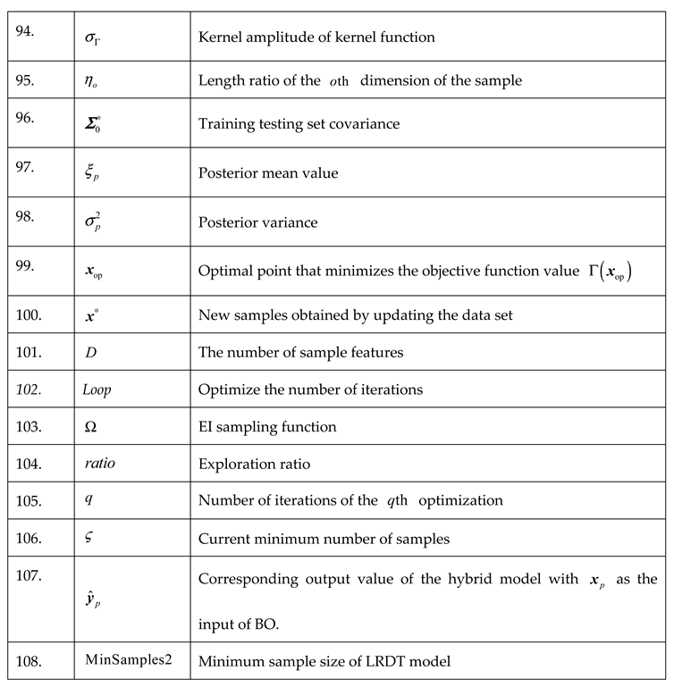
This study is based on an MSWI plant of typical grate furnace in Beijing. Its process flow is shown in Figure 1.
Figure 1 shows that this MSWI procss mainly includes six process stages: solid waste fermentation, solid waste combustion, waste heat exchange, flue gas cleaning, flue gas emission, and steam power generation [35,36]. The detailed description is as follows.
(1)Solid waste fermentation stage. The original MSW contains a large amount of water, which is not conducive to combustion. Therefore, it needs to be bio-fermented in a solid waste reservoir. This process can increase the calorific value of the solid portion by about 30% with about 5-7 days. Then, the fermented MSW transfers it to the hopper and pushes into the incinerator by the feeder and enters the solid waste combustion stage.
(2)Solid waste combustion stage. This stage is to convert MSW into high temperature under the coupling interaction of multi-phase such as solid-gas-liquid and multi-field such as heat flow force. It can be divided into three phases: drying, combustion and burnout. The dring phase is realized based on the furnace’s heat radiation phenomenon and the preheated primary air drying function. During combustion phase, MSW is ignited and produces flue gas. After about 1.5 hours of high-temperature combustion, the combustible components are fully burned and the enters the burnout phase. The non-combustible ash is pushed out of the furnace by the burnout grate.
(3)Waste heat exchange stage. Firstly, the high temperature flue gas is initially cooled by the water wall. Secondly, heat energy is transferred to the boiler by radiation and convection using equipment such as superheaters, evaporators and economizers. Then, the water in the boiler is converted into high-pressure superheated steam and enters the steam generation stage. Finally, the outlet flue gas temperature of the boiler is reduced to 200 °C. In this stage, the cooling rate needs to be strictly controlled to prevent the re-generation of pollutants.
(4)Steam power generation stage. Using the high temperature steam generated by the waste heat boiler. Converting mechanical energy into electrical energy to achieve self-sufficiency in plant-level electricity consumption and external supply of surplus electricity. At the same time, it also can realize resource utilization and obtain economic benefits.
(5)Flue gas cleaning stage. Firstly, the denitrification system is used to remove NOx. Secondly, the acid gas is neutralized by semi-dry deacidification process. Then, activated carbon is used to adsorb DXN and heavy metals in flue gas. Finally, the particles, neutralizing reactants and activated carbon adsorbates in the flue gas are removed by the bag filter.
(6)Flue gas emission stage. The flue gas that meets the national emission standards is discharged into the atmosphere through the chimney through the induced draft fan.
The key controlled variables involved in the solid waste combustion stage are furnace temperature, flue gas oxygen content, steam flow and combustion line. This stage includes three processes: drying, combustion and burnout. In the combustion process, a strong oxidation reaction occurs, indicating that the combustible component and oxygen undergo a complete combustion reaction. Obviously, the oxygen content (air supply volume) and MSW feed rate (grate speed) in the combustion process are crucial to the combustion process. In the burnout process, under the action of high temperature and primary air, the coke will oxidize with oxygen. Therefore, maintaining the stability of flue gas oxygen content is of great significance for the stable operation of combustion process.
2.2. Flue Gas Oxygen Content Control Description
In the MSWI process, flue gas oxygen content is a characterization of the excess oxygen air coefficient. It can characterize the combustion state to a certain extent [1]. When flue gas oxygen content is too low and the excess air ratio is too low, a large amount of toxic and harmful gases will be produced in addition to the increase of heat loss and the decrease of combustion efficiency [7]. When flue gas oxygen content is too large and the excess air coefficient is too large, it shows that the amount of air is too large. The excess air can take away a lot of heat and dust, i.e., high flue gas oxygen content, also increase the emission of NOx pollutants [7].
Normally, the flue gas oxygen content at the outlet of the waste heat boiler is taken as one of the key controlled variables to reflect the MSWI process. Only when flue gas oxygen content is controlled within a certain range, it is possible to make the MSW and combustible flue gas in the furnace fully burned. Thus, the emission concentration of secondary pollutants can be ensure to meet the environmental standards. Therefore, it is of great significance to establish an accurate controlled object model of flue gas oxygen content to support the research of related intelligent control algorithms to realize the smooth, efficient and environmentally friendly operation of MSWI process [8].
The MSWI process is complex, and there are many variables that affect the O2 at the outlet of the waste heat boiler, and some of them are coupled. Therefore, first of all, the variables are preliminarily selected according to the expert experience [37]. The primary air volume, secondary air volume, feeder speed average, drying grate speed average and ammonia injection amount are selected as MVs. In addition, because the mechanism model is difficult to construct, the construction of data-driven model is the current research hotspot. Without affecting the normal operation of the industrial site, collecting process data for modeling at the same time is the first problem to be solved in building the model.
2.3. Data Acquisition Devices Description and Experimental Data Analysis
Usually, in order to ensure the safe and reliable operation of the MSWI process, DCS systems with closed characteristics in industrial sites are strictly integrated with external devices for data collection and algorithm testing. To address this issue, we collected data using an edge verification platform of MSWI power plant equipped with a safety isolation acquisition device as shown in Figure 2.
The device in Figure 1 facilitates one-way data transmission, mitigating interference issues during the data acquisition process. The industrial data for the experiment are obtained from an actual MSWI power plant in Beijing, China, with a collection frequency of 1 second. 16 hours of continuous process data from 8:00 to 24:00 on a certain day are used. The data are processed through moving averages to eliminate outliers, 857 samples were generated and used to build the FT controlled object model. Further, we divide these samples into training set and testing set in a ratio of 3:1.
There are five key MVs (primary air volume, secondary air volume, feeder speed average, drying grate speed average and ammonia injection amount) and one controlled variable (CV) (flue gas oxygen content). Pearson correlation coefficient ( PCC ) is used to evaluate the correlation between the key MVs and the CV, as shown in Figure 3.
Figure 3 shows that there is a strong linear relationship between ammonia injection amount and flux gas oxygen content for the modeling data used in this article. Obviously, the flux gas oxygen content of the actual MSWI process should have a stronger mapping relationship with other MVs. Since PCC can only measure the linear relationship between MVs and CVs, Figure 3 also indicates that there is a complex nonlinear or even uncertain mapping relationship between flux gas oxygen content and MVs. Therefore, it is necessary to adopt a modeling strategy that can characterize strong uncertainty and complex mapping relationships to construct a controlled object model for flux gas oxygen content.
2.4. Modeling Strategy
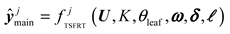
Based on the previous analysis, it can be concluded that constructing a flue gas oxygen content model for the MSWI process is the foundation for implementing stable control algorithms. In this article, an interpretable flue gas oxygen content based on BO-EnTSFRT-LSTM is proposed. In which, the main model is constructed by using EnTSFRT to model the uncertainty, the LSTM is used to construct the compensation model by using the main model error as the true value, and the hyperparameters of the constructed main-complement ensemble model are optimized based on the BO algorithm. The overall modeling strategy is shown in Figure 4.
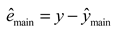
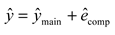
In Figure 3, where denotes MVs, represents the true value of flue gas oxygen content, represents the output value of EnTSFRT main model, represents the error value of EnTSFRT main model, denotes the output value of LSTM compensation model, denotes the error value of LSTM compensation model, represents the output value of BO-EnTSFRT-LSTM. The relationships among above the variables are as follow:
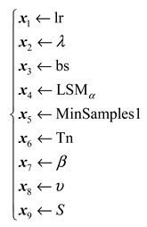
In addition, , , , , , , , and in Figure 4 represent the hyperparameters of the main-complement ensemble model that the BO algorithm needs to optimize. They are learning rate, number of batches, the intermediate variable in the recursive calculation process, regularization coefficient, the minimum number of samples and the number of decision trees of the main model and the learning rate, regularization coefficient and maximum number of iterations of the compensation model, respectively.
The functions of different modules are as follows:
1) Main model construction module based on EnTSFRT: It is obtained by constructing multiple TSFRT sub-models with parallel fusion mode;
2) Compensation model construction module based on LSTM: It is used to construct the compensation model with the error true value of the EnTSFRT model;
3) Hyperparameter optimization module based on BO algorithm: The hyperparameters of the constructed main-complement ensemble model are optimized based on the BO algorithm.
2.5. Algorithm Implementation
2.5.1. Main Model Construction Module Based on EnTSFRT
The EnTSFRT model requires parallel fusion of multiple TSFRT sub-models. The TSFRT sub-model mainly includes a screening layer and a fuzzy inference layer. Among them, the screening layer is used for feature screening, and the fuzzy inference layer uses TS fuzzy inference.
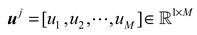
where denotes the input of EnTSFRT, denotes MVs, denotes the input sample, represents the total number of data set samples, represents dimension of the input feature, represents the input variable matrix of the subset sample, denotes the training subset obtained by random feature sampling of , and denote the membership degree on the non-leaf nodes of and , denotes the TSFRT sub-model.
2.5.1.1. Training Subsets Partition Submodule
The training subset of features is obtained by feature random sampling of . It can be expressed as:
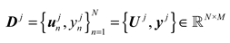 where denotes the input variable matrix, represents the true value vector of flue gas oxygen content.
Correspondingly, from the perspective of input features, with input features can be expressed as:
Therefore, a subset denoted as can be obtained.
2.5.1.2. Sub-Model Construction Submodule
The construction of the TSFRT sub-model is described as an example.
The data set is used as the input of the screening layer. And the best segmentation position is determined. Each recursive coordinate point in is obtained. And its mean square error (MSE) value is calculated to minimize MSE to determine the segmentation node. The estimation process of the loss function value is as follows:
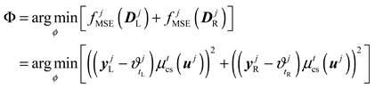 where represents the loss value of data set , denotes the MSE value of the left subset (or right subset ), denotes the true vector of the left subset , denotes the true vector of the right subset , denotes the clear membership function of the input on the non-leaf node, represents the average of the target values of the left subset , represents the average of the target values of the right subset .
In this article, both and are represented as . Its calculation is as follows:
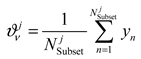 where denotes the number of (or ).
In Equation (5), is calculated as:
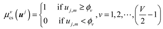 where denotes the clear membership function of the input , indicates that the segmentation threshold can be expressed as . It is assumed that the TSFRT sub-model in this article consists of nodes. So, the number of non-leaf nodes is , and the sum of membership sets is .
is divided into left and right subsets as follows:
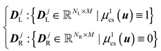 where denotes the first membership degree of a clear set obtained by using the minimum MSE. The first element of the clear set is defined by Equation (7). The clear set is described as:
Repeat the previous step until the minimum number of samples at the leaf node reaches the set threshold. The clear set can be expressed as:
It can be further expressed as:
The training data of the node is determined according to . And the T-S fuzzy inference is constructed. denotes the following:
 where represents the training data of fuzzy reasoning, denotes the leaf node, and denotes the number of samples in the leaf node.
In the fuzzy inference layer, rules are defined to represent the local linear relationship between the input variable and the target. Define the rule as follows:
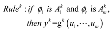
where represents the output of the consequent of the fuzzy rule, that is, the weight of the fuzzy rule. Further, we simplify Equation (13) as follows:
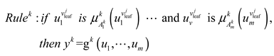 where denotes a variable of , denotes the membership degree of the fuzzy rule, denotes the membership function of , and describes the membership of to .
In the article, Gaussian function is used as membership function, as follows:
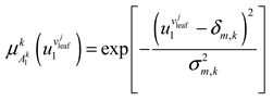 where denotes the center of the membership function, and represents the width of membership function.
The activation intensity of the fuzzy rule of the fuzzy rule of input variables is calculated as follows:
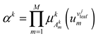 where denotes the product output of the fuzzy rule.
Further normalization operation is as follows:

According to Equations (13)–(17), and are linearly combined and accumulated. The predicted output values are obtained as follows:
 where represents the consequent output function, and denotes the consequent weight parameter.
Repeat the above steps until leaf nodes are obtained. By obtaining fuzzy inferences to construct a multi-input single-output model, the TSFRT simplified model of multi-input single-output can be obtained as follows:
 where denotes the TSFRT sub-model, , denotes the minimum number of samples, denotes the consequent weight parameter matrix, represents the center matrix of membership function, represents the width matrix of membership function.
In addition, the article uses the least squares method to update the weight of the consequent. Equation (18) can be merged as follows:
 where .
Given the input and output matrices, the T-S consequent weights can be estimated as follows:
 where is composed of .
The least square method is used for parameter learning. The recursive calculation is as follows:
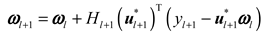
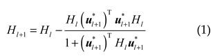 where is the weight of the initial time, which is a random vector; denotes the recursive process; is the intermediate variable in the recursive process; is defined by , denotes a large positive value, and represents the unit matrix.
2.5.1.3. Parallel Fusion Submodule
Firstly, according to the modeling process of TSFRT, total TSFRT models are constructed, which are defined as .
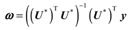
Then, to estimate the weight with the minimum training error, the following optimal problem is used to calculate the pseudo-inverse:
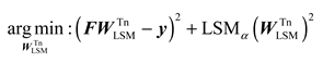 where denotes the regularization coefficient.
Using the ridge regression theory, that is, the Moore-Penrose inverse matrix, the weight matrix is calculated. The calculation results are as follows:
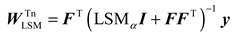
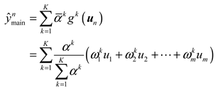
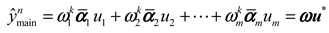
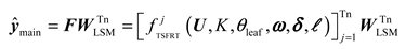
Finally, the output of EnTSFRT is as follows:
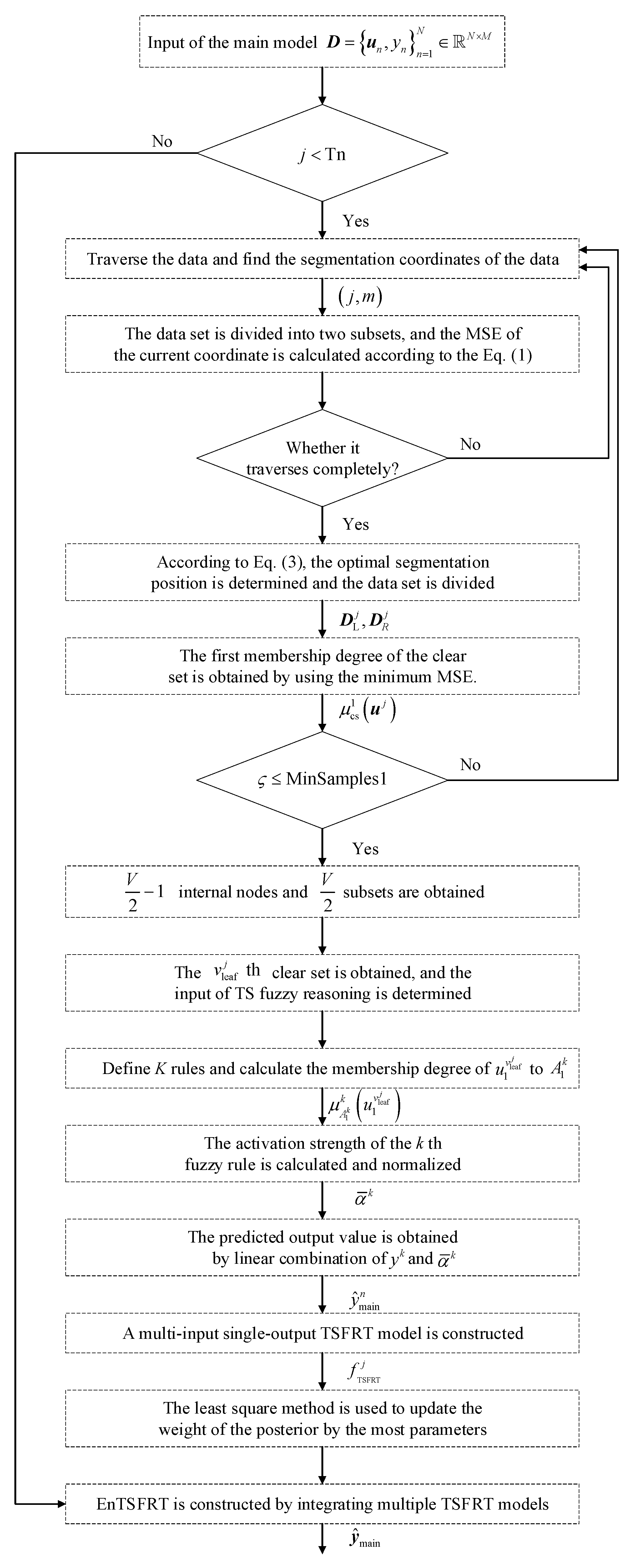
2.5.1.4. Flow Chart of Main Model Modeling
The flow chart of the construction of the main model is as follows:
Figure 6.
The flow chart of the construction of the main model.
2.5.2. Compensation Model Construction Module Based on LSTM
LSTM is a special recurrent neural network (RNN). The difference is that LSTM introduces three gates of forget gate, input gate and output gate and one cell state. The structure of LSTM is shown as follows :
Figure 7.
Structure of compensation model construction module based on LSTM.
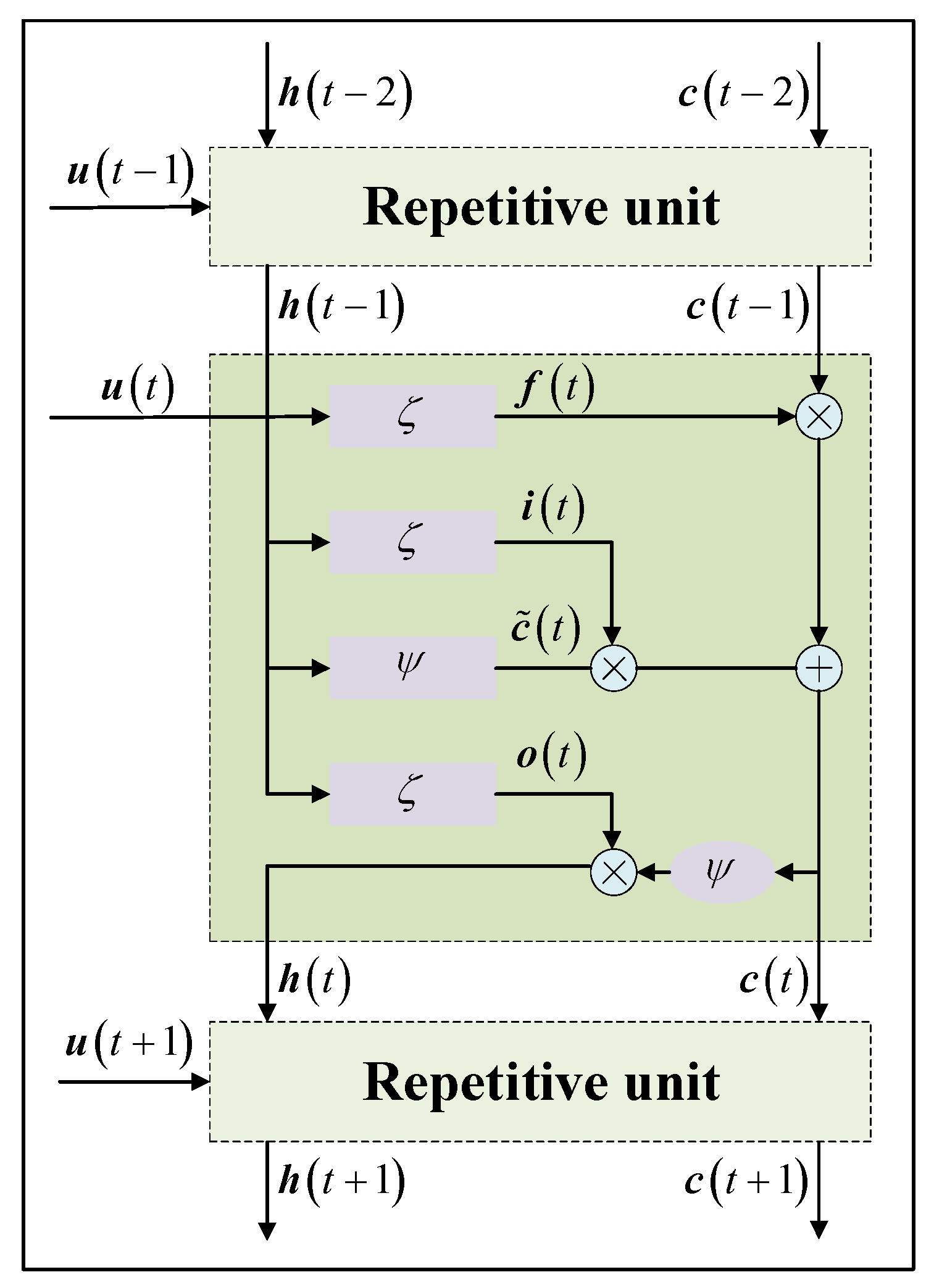
where denotes the current moment, denotes the hidden state, denotes the cell state, denotes the candidate cell state, represents the sigmoid function, represents the tanh function, denotes the value of the forget gate, denotes the value of the input gate, represents the value of the output gate, represents element-by-element multiplication.
Its forward calculation and back propagation are as follows.
2.5.2.1. Forward Calculation Process
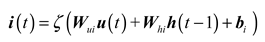
The output of forget gate, input gate, output gate, candidate cell state, cell state and hidden state can give the network memory ability of repetitive unit [7]. The forward calculation process at time are as follows.
Firstly, update the output of the forget gate as follows:
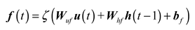 where represents the weight matrix, represents the bias matrix.
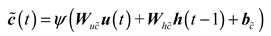
Secondly, the output of the input gate is updated and new candidate cell state is generated, as follows:
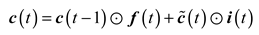
Further, the cell state is updated as follows:
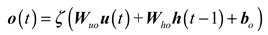
Then, the output gate is updated and the cell state at the current moment is generated, as follows:
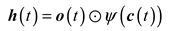
Finally, the output value of LSTM is obtained as follows :
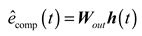 where is the output weight matrix.
2.5.2.2. Back Propagation Process
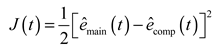
The loss function in the training process of LSTM is defined as follows:
The weights and biases are updated based on the back propagation algorithm. Taking the update of as an example, as follows:
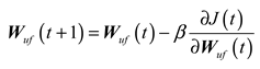
Using the chain rule, is calculated as follows:
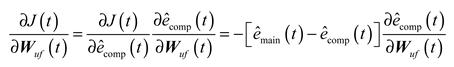
The calculation of is as follows :
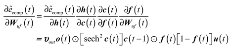
Further, can be obtained.
The update process of the remaining weights and biases is the same as the update process of .
2.5.2.3. Flow Chart of Compensation Model Modeling
The flow chart of the construction of the compensation model is as follows:
Figure 8.
The flow chart of the construction of the compensation model.
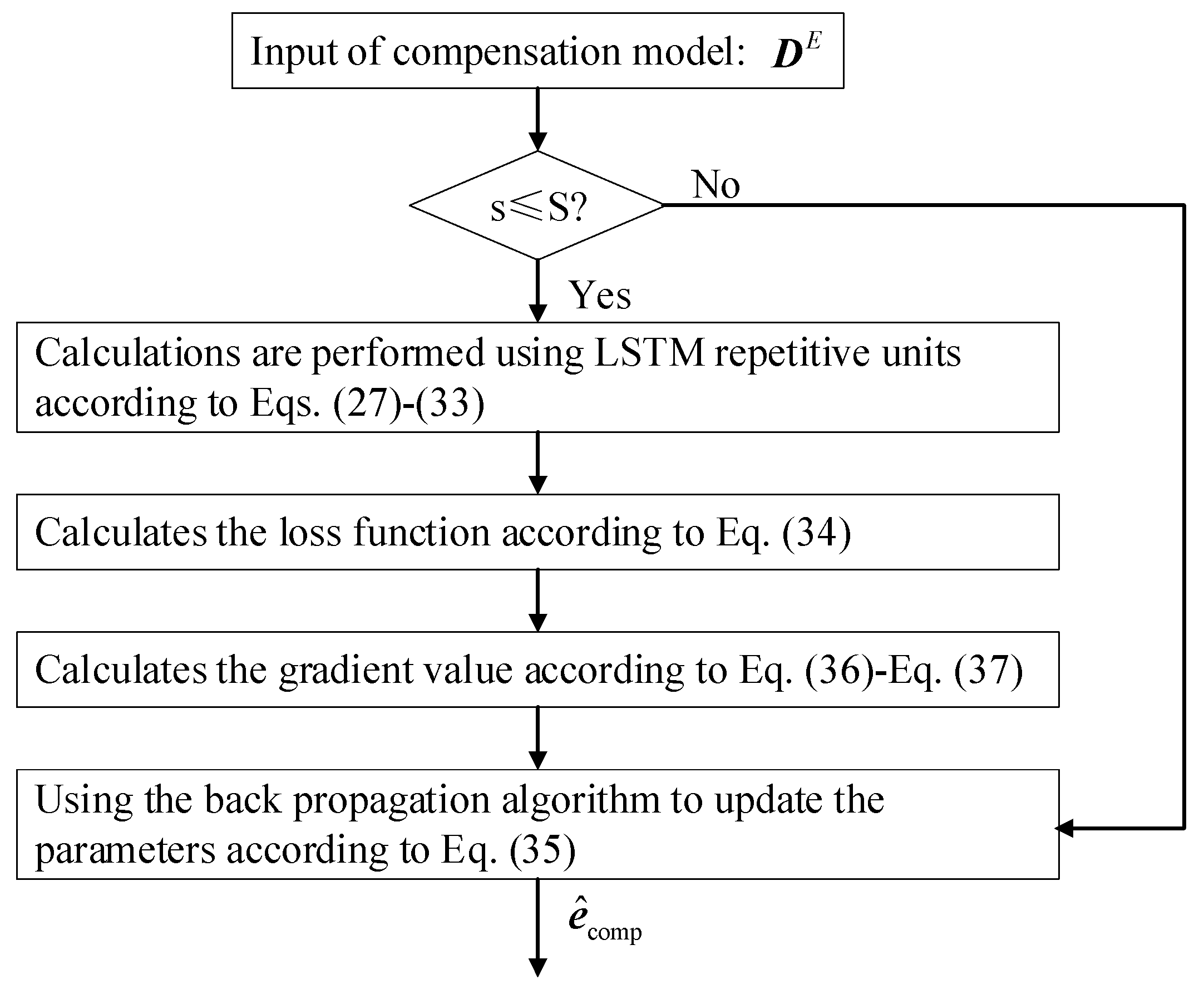
where is the input of the compensation model, denoted as ; and represents the iteration number.
2.5.3. Hyperparameter Optimization Module Based on BO Algorithm
2.5.3.1. The Principle of BO Algorithm
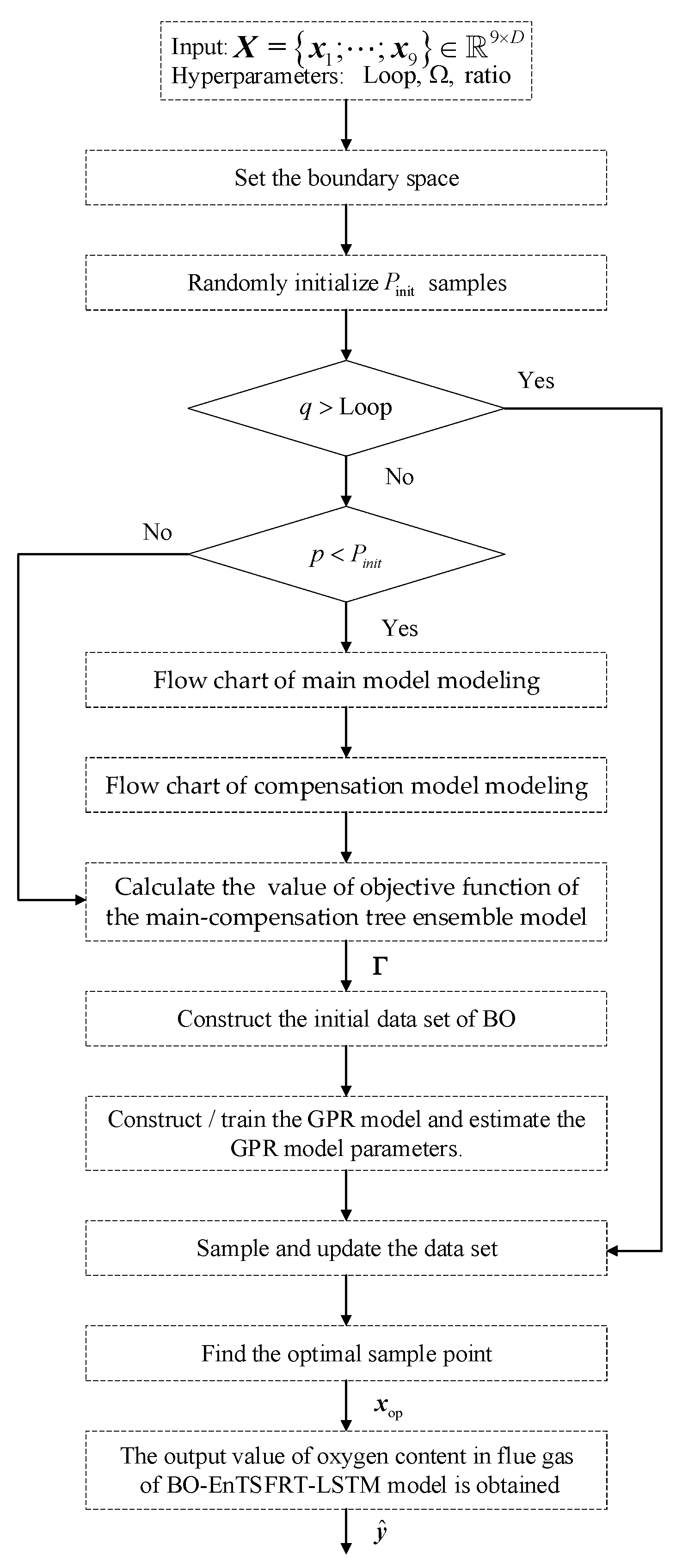
BO is a kind of optimization method based on machine learning. Its purpose is to minimize the objective function. In the article, the eight hyperparameters in the main complement ensemble model are selected based on the BO algorithm to achieve the purpose of minimizing the objective function. The objective function selected in this article is the negative vaue of R-square (R2) indicator.
The optimization process of BO algorithm is as follows.
Step 1: Set the boundary space
Set the value range of the hyperparameters of BO. It includes the upper boundary (UB) and the lower boundary (LB) of the sample space, which is set as follows:
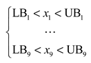 where denotes as follows:
Step 2: Construct the initial data set
Randomly initialize input samples . And observe the corresponding objective function value of the sample to form the initial data set.
Step 3: Construct / train the GPR model
The Gaussian process regression (GPR) model is constructed by using the data set. The GPR model uses the known data as a prior probability distribution that satisfies the multivariate normal distribution. It is described as follows:
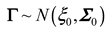 where is the mean function, represents the number of data set samples at the current time, and denotes the covariance matrix as follows:
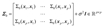 where represents the variance of the measurement noise, is the kernel function between the and sample points. It is calculated as follows:
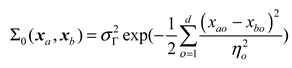 where represents the dimension feature of the sample, is the kernel amplitude of the kernel function, denotes the length ratio of the dimension of the sample.
For a new sample point in the sample space, the posterior probability distribution of the sample point can be calculated by the prior probability distribution. According to the definition of GP, the joint Gaussian distribution and the predicted value of the known data also obey the Gaussian distribution, which can be expressed as:
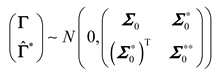 where represents the covariance of training testing set, and denotes the covariance of the testing set.
Since the training set is known, the conditional distribution for given can be calculated based on Equation (43) as follows:
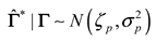 where and are as follows:
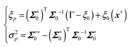 where is the posterior mean value, and denotes the posterior variance.
Step 4: Estimate the parameters of the GPR model
We estimate the parameters in the mean function and covariance matrix. Maximum likelihood estimation (MLE) is used to estimate the above parameters, which improves the fitting and prediction performance of the model [38,39].
Step 5: Sampling
In order to find the optimal point to minimize the objective function value , the expected improvement (EI) sampling function is used to sample the objective function.
Step 6: Update the data set
We calculate the objective function value corresponding to the new sample point . Then, we update the data sets and .
Repeat steps 3-6 until the preset maximum number of iterations is reached. And find the optimal sample point that meet the requirements from the dataset.
2.5.3.2. The Flow Chart of BO Algorithm
The flow chart of BO algorithm is as follows:
Figure 9.
The flow chart of BO algorithm.
2.6. pseudo code
The pseudo code of the pseudocode algorithm used in this article is as follows:
where represents the number of optimization iterations, represents the sampling function, represents the exploration ratio, is the current minimum number of samples.
Table 1 shows that the parameters of BO process are , , and . Among them, BO establishes a probability model based on the past evaluation results of the objective function and finds the value that minimizes the objective function. The commonly used sampling functions include: expectation boosting, knowledge gradient, and entropy search and predictive entropy search. Its selection needs to consider how likely it is to obtain the optimal value at a certain point, and to evaluate whether the point can reduce the uncertainty of the Bayesian statistical model. The exploration ratio is a parameter that controls the balance between exploration and exploitation, and it needs to be adjusted according to specific optimization tasks and application scenarios.
3. Results and Discussion
3.1. Performance Metrics
The evaluation indexes used in the article are root mean squard error (RMSE), mean absolute error (MAE) and R-Square (R2), as follows:
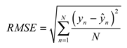
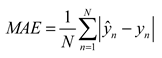
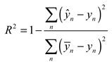 where RMSE represents the standard deviation of the sample for the difference between the predicted and true values, reflecting the degree of dispersion of the sample. MAE represents the average absolute error between the predicted and true values. And when doing nonlinear fitting, the smaller the RMSE, the better[40]. R2 is used to quantify the fitting degree of the model to the data. Generally speaking, the closer the value of R2 is to 1, the better the fitting degree of the model is.
3.2. Experimental Results
The parameters of BO are set based on Thumb rule. The detaied values are follows: , = EI function, and = 0.5. The optimal hyperparameters are selected as , , , , , , , and . The fitting curves of the training set and testing set of the main-compensation ensemble model are shown in Figure 10 and Figure 11.
According to Figure 10 and Figure 11, only using the EnTSFRT-based main model, the predicted value cannot fit the actual value effectively. The compensation model has a better fitting effect on the error value of the main model. At the same time, by comparing Figure 10(a)-Figure 11(a) with Figure 10(c)-Figure 11(c), it can be seen that the fitting effect of the proposed method on the training set and the testing set has a great improvement.
The weights of all trees constructed by the main model are shown in Figure 12:
The curve of the objective function in the BO optimization process is as follow:
Figure 13 shows that the value of the objective function is in the range of -0.5079 to -0.7988 in the BO optimization process.
The variation curves of the 9 hyperparameters in the BO optimization process are as follows:
Figure 14 shows the change process of hyperparameters of the main-complement ensemble model in the BO optimization process. The specific detailed analysis is as follow:
1) Figure 14(a) shows the change curves of , which is the learning rate of the main model. When the range of is 0 to 50, the change of is dramatic. When the range of is 50 to 280, the value of is basically stable at 0.18. When the is greater than 280, it first stabilizes at about 0.3. Then changes sharply and finally tends to be stable at about 0.18.
2) Figure 14(b) shows the change curves of , which is the intermediate variable in the recursive calculation process of the main model. With the increase of , its change trend is similar to that of . Its value is finally stabilized at about 16.
3) Figure 14(c) shows the change curves of , which is the the number of batches of the main model training. With the increase of , its change trend is similar to that of . Its value is finally stabilized at about 25.
4) Figure 14(d) shows the change curves of , which is the regularization coefficient of the master model. With the increase of , its change trend is similar to that of . Its value is finally stabilized at about 0.48.
5) Figure 14(e) shows the change curves of , which is the minimum number of leaf node samples of the main model. With the increase of , the value of first changed dramatically. Then its value is basically stable at about 41.
6) Figure 14(f) shows the change curves of , which is the number of decision trees of the main model. When is 0 to 20, changes drastically. When is greater than 20, the value of is stable at about 23.
7) Figure 14(g) shows the change curves of , which is the learning rate of the compensation model. With the increase of , the change trend of its value is similar to that of . Its value eventually converges to about 0.026.
8) Figure 14(h) shows the change curves of , which is the regularization coefficient of the compensation model. When is in the range of 0 to 40, its value fluctuates greatly. Then, its value converges to about 0.2. When is greater than 280, the value is mostly around 0.01.
9) Figure 14(i) shows the change curves of , which is the iteration times of the compensation model. When is in the range of 0 to 50, its value changes dramatically. When is greater than 50, its values converge to 328, 345 and 382 respectively.
3.3. Comparison and Discussion
To further illustrate the effectiveness, the proposed method is compared with tree-based method such as random forest (RF), LRDT, EnTSFRT-LRDT and BO-EnTSFRT. The hypeparameters of each model are set as follows. In RF model, the minimum number of samples is set to 50, and the number of features is 4. In LRDT model, the minimum number of samples is set to 20, and the regularization coefficient is 0.4. In EnTSFRT-LRDT model, , , , , , , , and . In EnTSFRT-LSTM model, , , , , , , , , . In BO-EnTSFRT model, , , , , , and . In BO-EnTSFRT-LRDT model, , , , , , , , and , where is the minimum sample size of LRDT model.
Based on the above models, the test is performed on the testing set, and repeated 20 times. One of the fitting curves and total statistical results are as follows.
It can be seen from Figure 15 that the fitting effect of the proposed method is the best based on different methods for the testing set. At the same time, it shows that the overall performance of the proposed method is the best one.
The calculation results of performance evaluation indexes of different methods are as follows.
Table 2 show the statistical results of performance evaluation indexes of different methods in terms of training set and testing set with 20 repeated times. The proposed BO-EnTSFRT-LSTM model has the lowest average RMSE and MAE for the training set (2.6610E-02, 2.0684E-02) and the testing set (4.3991E-01, 3.1771E-01). At the same time, the proposed method has the highest R2 on the training set (9.9896E-01) and the testing set (7.5649E-01±2.4804E-04). By comparing the method proposed in this article with EnTSFRT-LSTM and BO-ENTSFRT, the important role of BO algorithm and LSTM-based compensation model is illustrated respectively. In addition, the comparison between the proposed method and the BO-EnTSFRT-LRDT further illustrates the superiority of the LSTM algorithm. The proposed BO-EnTSFRT-LRDT method utilizes EnTSFRT to handle uncertainty in industrial modeling data, fits error data using LSTM, and avoids hyperparameters that are prone to overfitting using BO, resulting in optimal modeling performance. By comparing with other methods, the superiority of the proposed method is proved.
Through the above comparative experiments and causal analysis, it indicates that the proposed method has the best performance compared to BO-EnTSFRT-LSTM-based modeling methods used in this study.
3.4. Hyperparameter Discussion
In the article, the single factor sensitivity analysis of the hyperparameters optimized by BO algorithm is carried out. Since the objective function of the BO algorithm is the negative value of the R2 of the ensemble model, the hyperparameters are changed according to a certain step size in the range of hyperparameters and negative value of R2 of the testing set are recorded for analysis. In the article, a total of 10 sets of experiments are set for each hyperparameter. The interval setting is as shown in Table 3:
The selection of step size should consider the sensitivity of hyperparameters and the limitation of computing resources. In this article, the experiment is carried out in a fixed step size according to the setting interval of the hyperparameters based on author’s debug experience and PC hardware performance. For of the main model, the initial value is set to 0.1, and the step size is 0.1; the initial value of is 3 and the step size is 3; the initial value of is 5 and the step size is 5; the initial value of is set to 0.1, and the step size is 0.1; the initial value of is 10 and the step size is 10; the initial value of is 20, and the step size is 20. For the of the compensation model, the initial value is 0.01 and the step size is 0.01; the initial value of is 0.05, and the step size is 0.1; the initial value of is 220, and the step size is 400. In the experiment, the single factor analysis strategy is used. By performing 20 repeated experiments, the mean and variance change curves of RMSE on the testing set are shown in Figure 16.
Figure 16 shows a single factor-based hyperparameter analysis for mean and variance of R2 in terms of average value of 20 times, and the results indicate that different hyperparameters of the constructed BO-EnTSFRT-LSTM model have different effects. The specific detailed analysis is as follow:
1) Figure 16(a) shows the effect of on the performance of the BO-EnTSFRT-LSTM model. When is less than 0.8, the mean value of R2 fluctuates in a small range. When is greater than 0.8, R2 decreases rapidly. It shows that it is easier to meet the requirements when is small. If the learning rate is too large, it may lead to skipping the optimal solution, which makes the model unable to achieve the best performance.
2) Figure 16(b) shows the effect of on the performance of the BO-EnTSFRT-LSTM model. When is in the range of 0 to 15, the mean value of R2 generally shows a rapid growth. And when its value is in the range of 15 to 27, only a small fluctuation is produced. At the same time, the variance in this range also shows an overall downward trend. It shows that it is easier to meet the conditions when the value of is larger.
3) Figure 16(c) shows the effect of on the performance of the BO-EnTSFRT-LSTM model. With the increase of , the mean and variance of R2 have relatively large fluctuations. It shows that the influence of on the performance of the model is more complicated and needs to be determined in combination with other hyperparameters.
4) Figure 16(d) shows the effect of on the performance of the BO-EnTSFRT-LSTM model. With the increase of , the mean value of R2 increases rapidly. When is in the range of 0.3 to 0.7, its value shows a decreasing trend as a whole. When is 0.7, the mean value of R2 is the smallest (0.7029). And then the mean value of R2 increases rapidly. At the same time, the variance of R2 also shows a downward trend.
5) Figure 16(e) shows the effect of on the performance of the BO-EnTSFRT-LSTM model. When the value of is greater than 30, the mean and variance of R2 fluctuate in a small range. And when , the mean value of R2 is the largest (0.7077) and the variance of R2 is small (0.0008209). It shows that the larger is easier to obtain higher performance model.
6) Figure 16(f) shows the effect of on the performance of the BO-EnTSFRT-LSTM model. When is in the range of 20 to 80 and 100 to 160, the mean value of R2 decreases rapidly. And when tn is 20, the mean value of R2 is the largest (0.7096) and the variance of R2 is small (0.0008537). It shows that it is easier to obtain a high performance model when is small.
7) Figure 16(g) shows the effect of on the performance of the BO-EnTSFRT-LSTM model. When the value of is 0.02, the mean value of R2 is largest (0.7206) and the variance value of R2 is smallest (0.0006435). When the value of is greater than 0.07, the learning rate is too large, resulting in gradient explosion. Therefore, in order to avoid the occurrence of gradient explosion, a smaller should be selected.
8) Figure 16(h) shows the effect of on the performance of the BO-EnTSFRT-LSTM model. When is less than 0.8, the mean fluctuation range of R2 is small. When is 0.5, the mean value of R2 is the largest (0.7152) and the corresponding variance is the smallest (0.0004927). And when is greater than 0.8, the mean value of R2 decreases rapidly.
9) Figure 16(i) shows the effect of on the performance of the BO-EnTSFRT-LSTM model. When is in the range of 220 to 340, the mean value of R2 fluctuates in a small range. The mean value of R2 increases rapidly when is in the range of 340 to 380. And when is 380, the mean value of R2 is the largest (0.7306).
It should be noted that the sensitivity analysis conducted here is based on single factor hyperparameters. In fact, these numerous hyperparameters are interdependent, which is one of the reasons why BO is used for hyperparameter selection in this article.
3.5. Comprehensive Analysis
For the method proposed in this article, there are some limitations in each stage as follows.
(1) When the main model is constructed, it consists of multiple decision trees, and the training and prediction process consumes a lot of computing resources. Further research is needed on how to perform structural reduction on the constructed decision tree based main model. Moreover, how to further enhance the model’s ability to represent uncertainties in the data also needs to be strengthened.
(2) When constructing the compensation model, the problem of gradient disappearance or gradient explosion may occur. At the same time, the structure of LSTM is complex and the training process is slow. Therefore, the structure of the model can be improved by researching its lightweight algorithms in the future.
(3) In the process of hyperparameters optimization, it is easy to fall into local optimum. For high-dimensional and non-convex functions with unknown smoothness and noise, it is often difficult for BO algorithm to fit and optimize them. How to improve the BO algorithm to enhance its ability and adaptability to the above problems is a problem that needs to be solved. In addition, further consideration is needed on how to perform BO optimization on non-gaussian distributed data.
4. Conclusion
The stable control of flue gas oxygen content during MSWI process is beneficial to improve incineration efficiency and reduce pollutant emissions. Aiming at the problem of lack of high-precision and interpretable flue gas oxygen content model, the article proposes a flue gas oxygen content model based on BO-optimized main-complement ensemble algorithm. The main contributions are as follows: (1) A hybrid model integrating parallel fusion and main-complement ensemble is proposed. (2) The strategy of using BO to optimize the hyperparameters of the main-complement ensemble model is proposed. (3) An interpretable and high-precision controlled object model for flue gas oxygen content is constructed for the first time. Experiments show that the performance of the proposed method is better than other methods, which shows the feasibility and effectiveness of the proposed method. In the subsequent research, the control algorithm will be carried out on this basis to ensure the efficient and stable operation of the MSWI process.
In addition, there are some limitations in this article. Due to the use of TSFRT and LSTM, this model consumes a lot of computer resources in its training stage. At the same time, how to improve the ability and adaptability of the BO algorithm to the above problems is a problem that needs to be solved. In addition, further consideration is needed on how to perform BO optimization on non-gaussian distribution industrial data.
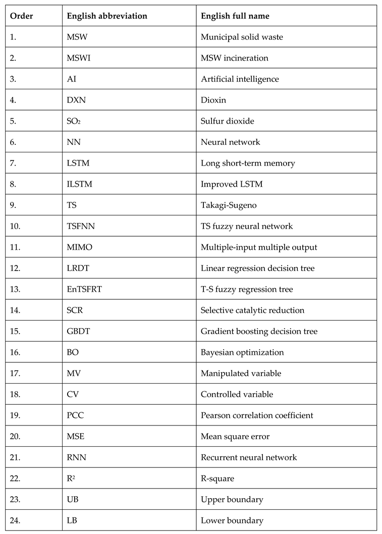
Appendix

Table A1.
Abbreviations and their meanings.
|
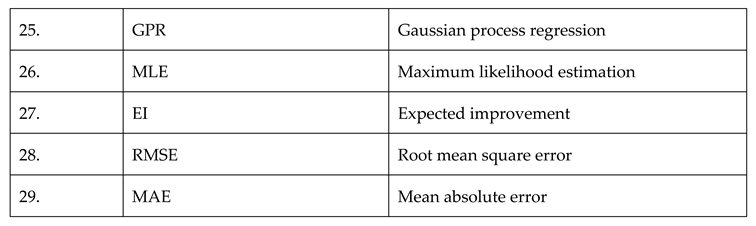
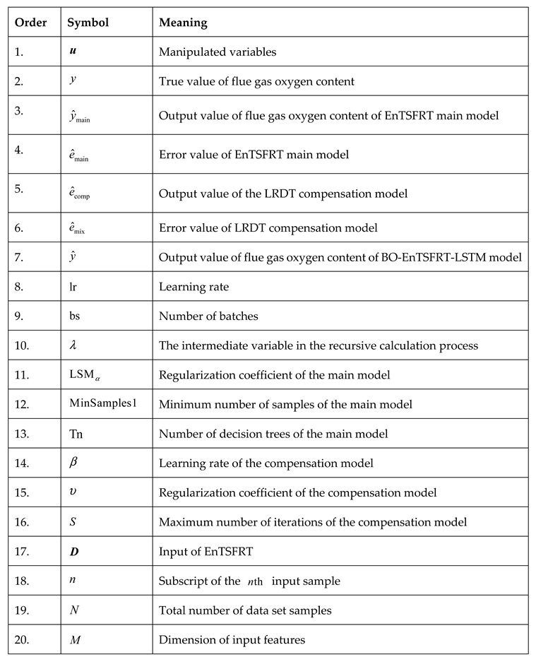
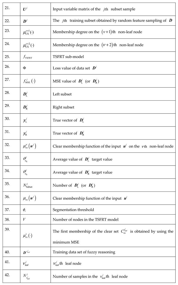
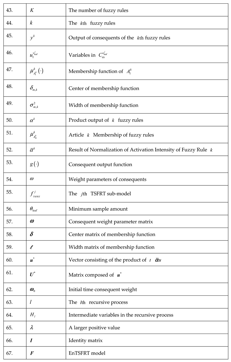
Table A2.
symbols and their meanings.
   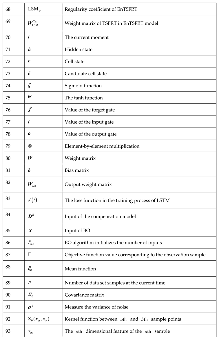 
|
References
- Jian, T.; Heng, X.; Wen, Y.; Jun-Fei, Q. Research status and prospect of intelligent optimization control of municipal solid waste incineration process. Acta Automatica Sinica 2023, 49, 2019–2059. [Google Scholar]
- An, C.; Jing-Rui, C.; Jing, C.; Chao, F.; Wei, W. Research on risks and countermeasures of “cities besieged by waste” in China-an empirical analysis based on DIIS. Bulletin of Chinese Academy of Sciences 2019, 34, 797–806. [Google Scholar] [CrossRef]
- Efforts to Promote the Realization of Carbon Peak Carbon Neutral Target. [Online]. Available: https://www.ndrc.gov.cn/wsdwhfz/202111/t20211111_1303691.html.
- Ding, H.; Tang, J.; Qiao, J. (2021). Control Methods of Municipal Solid Wastes Incineration Process: A Survey. In 2021 40th Chinese Control Conference (CCC)(pp. 662-667). IEEE.
- Can-Lin, C.; Jian, T.; Heng, X.; Jun-Fei, Q. Early warning of dioxin emission in municipal solid waste incineration process based on fuzzy neural network confrontation generation. Control Theory & Applications 2024, 1–9.
- Pan, X.; Tang, J.; Xia, H. (2023). Flame combustion state identification based on CNN in municipal solid waste incineration process. In 2023 5th International Conference on Industrial Artificial Intelligence (IAI)(pp. 1-4). IEEE.
- Qiao, J.; Sun, J.; Meng, X. Event-triggered adaptive model predictive control of oxygen content for municipal solid waste incineration process. IEEE Transactions on Automation Science and Engineering 2024, 21, 463–474. [Google Scholar] [CrossRef]
- Jian, S.; Xi, M.; Jun-Fei, Q. Data-driven predictive control of flue gas oxygen content in municipal solid waste incineration process. Control Theory & Applications 2024, 41, 484–495. [Google Scholar]
- Kai-Cheng, H.; Ai-Jun, Y.; Jian, T. Multi-objective robust prediction model of furnace temperature and flue gas oxygen content in municipal solid waste incineration process. Acta Automatica Sinica 2024, 50, 1001–1014. [Google Scholar]
- Huang, W.; Ding, H.; Qiao, J. Adaptive multi-objective competitive swarm optimization algorithm based on kinematic analysis for municipal solid waste incineration. Applied Soft Computing 2023, 149, 110925. [Google Scholar] [CrossRef]
- Sun, J.; Meng, X.; Qiao, J. Event-Based Data-Driven Adaptive Model Predictive Control for Nonlinear Dynamic Processes. IEEE Transactions on Systems Man and Cybernetics: Systems 2024, 54, 1982–1994. [Google Scholar] [CrossRef]
- Li, L.; Ding, S.; Yang, Y.; Peng, K.; Qiu, J. A fault detection approach for nonlinear systems based on data-driven realizations of fuzzy kernel representations. IEEE Transactions on Fuzzy Systems, 26, 1800-1812. [CrossRef]
- Cho, S.; Kim, Y.; Kim, M.; Cho, H.; Moon, I.; Kim, J. Multi-objective optimization of an explosive waste incineration process considering nitrogen oxides emission and process cost by using artificial neural network surrogate models[J]. Process Safety and Environmental Protection 2022, 162, 813–824. [Google Scholar] [CrossRef]
- Sildir, H.; Sarrafi, S.; Aydin, E. Optimal artificial neural network architecture design for modeling an industrial ethylene oxide plant. Computers & Chemical Engineering 2022, 163, 107850. [Google Scholar] [CrossRef]
- Rahimieh, A.; Mehriar, M.; Zamir, S.; Nostrati. Fuzzy-decision tree modeling for H2S production management in an industrial-scale anaerobic digestion process. Biochemical Engineering Journal 2024, 208, 109380. [Google Scholar] [CrossRef]
- Ma, Y.; Zhou, Y.; Peng, J.; Chen, R.; Dai, H.; Ma, H.; Hu, G.; Xie, Y. Prediction of flue gas oxygen content of power plant with stacked target-enhanced autoencoder and attention-based LSTM. Measurement 2024, 235, 115036. [Google Scholar] [CrossRef]
- Hai-Xu, D.; Jian, T.; Heng, X.; Jun-Fei, Q. MIMO controlled object modeling of municipal solid waste incineration process based on TS-FNN. Control Theory & Applications 2022, 39, 1529–1540. [Google Scholar]
- Lin, C.; Lee, C. Neural-network-based fuzzy logic control and decision system. IEEE Transactions on Computers Institute of Electrical and Electronics Engineers 1991, 40, 1320–1336. [Google Scholar] [CrossRef]
- Wu, D.; Peng, R.; Mendel, J. Type-1 and interval type-2 fuzzy systems. IEEE Computational Intelligence Magazine 2023, 18, 81–83. [Google Scholar] [CrossRef]
- Tang, J.; Xia, H.; Zhang, J.; Qiao, J.; Yu, W. Deep forest regression based on cross-layer full connection. Neural Computing and Applications 2021, 33, 9307–9328. [Google Scholar] [CrossRef]
- Xia, H.; Tang, J.; Wang, T.; Tian, H.; Cui, C.; Yu, W. (2023). Interpretable controlled object model of furnace temperature for MSWI process based on a novle linear regression decision tree. In 2023 35th Chinese Control and Decision Conference (CCDC)(pp. 325-330). IEEE.
- Xia, H.; Tang, J.; Yu, W.; et al. Takagi–Sugeno Fuzzy Regression Trees With Application to Complex Industrial Modeling. IEEE Trans. Fuzzy Syst. Inst. Electr. Electron. Eng. (IEEE) 2023, 31, 2210–2224. [Google Scholar] [CrossRef]
- Meng, T.; Zhang, W.; Huang, J.; Cui, C.; Qiao, J. Fuzzy reasoning based on truth-value progression: A control-theoretic design approach. International Journal of Fuzzy Systems 2023, 25, 1559–1578. [Google Scholar] [CrossRef]
- Yang, T.; Ma, K.; Lv, Y.; Fang, F.; Chang, T. Hybrid dynamic model of SCR denitrification system for coal-fired power plant. (2019). In 2019 IEEE 28th International Symposium on Industrial Electronics (ISIE)(pp. 106-111). IEEE.
- Luo, A.; Liu, B. (2022). Temperature prediction of roller kiln based on mechanism and SSA-ELM data-driven integrated model. In 2022 China Automation Congress (CAC)(pp. 5598-5603). IEEE.
- Dong, S.; Zhang, Y.; Liu, J.; Zhou, X.; Wang, X. (2022). Intelligent compensation prediction of leaching process based on GRU neural network. In 2022 China Automation Congress (CAC)(pp. 1663-1668). IEEE.
- Xia, H.; Tang, J.; Yu, W.; Jun-Fei; Qiao. Dioxin emission modeling based on simulation mechanism and improved regression decision tree. Acta Automatica Sinica 2024, 50, 1001–1019. [Google Scholar]
- Friedman, J. Greedy function approximation: A gradient boosting machine. The Annals of Statistics 2001, 29, 1189–1232. [Google Scholar] [CrossRef]
- Wang, W.; Deng, C.-H.; Zhao, L.-J. Research on the application of ellipsoid bound algorithm in hybrid modeling. Acta Automatica Sinica 2014, 40, 1875–1881. [Google Scholar]
- Duan, H.; Meng, X.; Tang, J.; Qiao, J. NOx emission prediction for MSWI process based on dynamic modular neural network. Expert Systems with Applications 2023, 238, 122015. [Google Scholar] [CrossRef]
- Zhang, R.; Tang, J.; Xia, H.; Chen, J.; Yu, W.; Qiao, J. Heterogeneous ensemble prediction model of CO emission concentration in municipal solid waste incineration process using virtual data and real data hybrid-driven. Journal of Cleaner Production 2024, 445, 141313. [Google Scholar] [CrossRef]
- Ma, S.; Chen, Z.; Zhang, D.; Du, Y.; Zhang, X.; Liu, Q. Interpretable multi-task neural network modeling and particle swarm optimization of process parameters in laser welding. Knowledge-Based Systems 2024, 300, 112116. [Google Scholar] [CrossRef]
- Zhou, X.; Tan, J.; Yu, J.; Gu, X.; Jiang, T. Online robust parameter design using sequential support vector regression based Bayesian optimization. Journal of Mathematical Analysis and Applications 2024, 540, 128649. [Google Scholar] [CrossRef]
- Deng, J.; Liu, G.; Wang, L.; Liu, W.; Wu, X. Intelligent optimization design of squeeze casting process parameters based on neural network and improved sparrow search algorithm. Journal of Industrial Information Integration 2024, 39, 100600. [Google Scholar] [CrossRef]
- Tian, H.; Tang, J.; Xia, H.; Wang, T.; Cui, C.; Pan, X. (2023). Furnace temperature control based on adaptive TS-FNN for municipal solid waste incineration process. In 2023 35th Chinese Control and Decision Conference (CCDC)(pp. 360-365). IEEE.
- Ding, H.; Tang, J.; Qiao, J. Dynamic modeling of multi-input and multi-output controlled object for municipal solid waste incineration process. Applied Energy 2023, 339, 120982. [Google Scholar] [CrossRef]
- Ding, H.; Tang, J.; Qiao, J. MIMO modeling and multi-loop control based on neural network for municipal solid waste incineration. Control Engineering Practice 2022, 127, 105280. [Google Scholar] [CrossRef]
- Rasmussen, C.E.; Williams, C.K.I. Gaussian Processes for Machine Learning[M].MIT Press,2005.
- Rasmussen, C.E. Gaussian Processes in Machine Learning;[C]//Advanced Lectures on Machine Learning, ML Summer Schools 2003, Canberra, Australia, February 2-14, 2003, Tübingen, Germany, August 4-16, 2003, Revised Lectures.2003.
- Wen-Ju,. Y., Ying-Dong,. Z.; Hong-Hua,. Y. Prediction of sediment discharge in Jinghe River based on optimized BP neural network. Journal of China Hydrology 2024, 1–8.
Figure 1.
MSWI process flow of typical grate furnace.
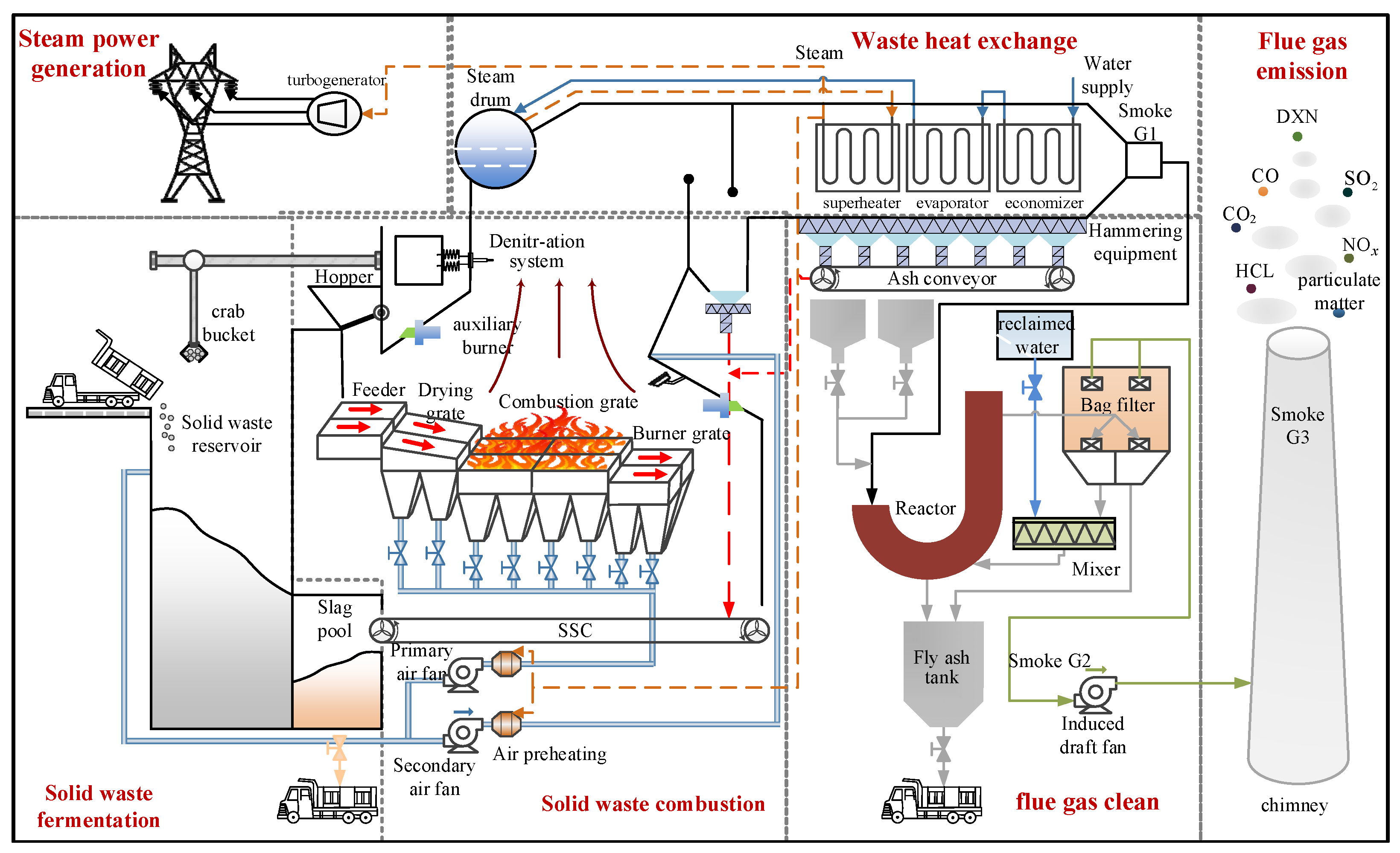
Figure 2.
Structure of edge verification platform of MSWI power plant.
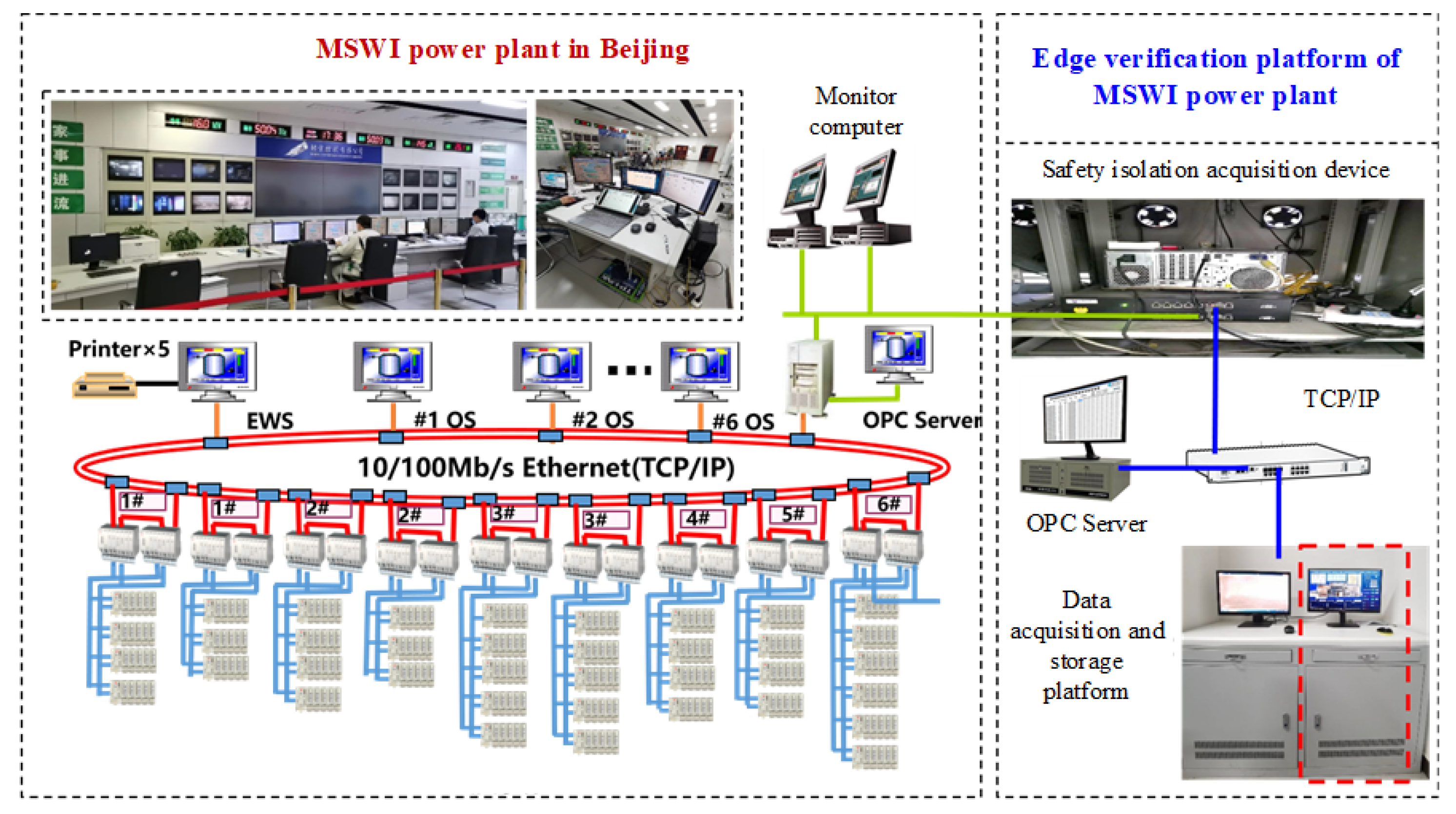
Figure 3.
PCC values between MVs and key flue gas oxygen content.
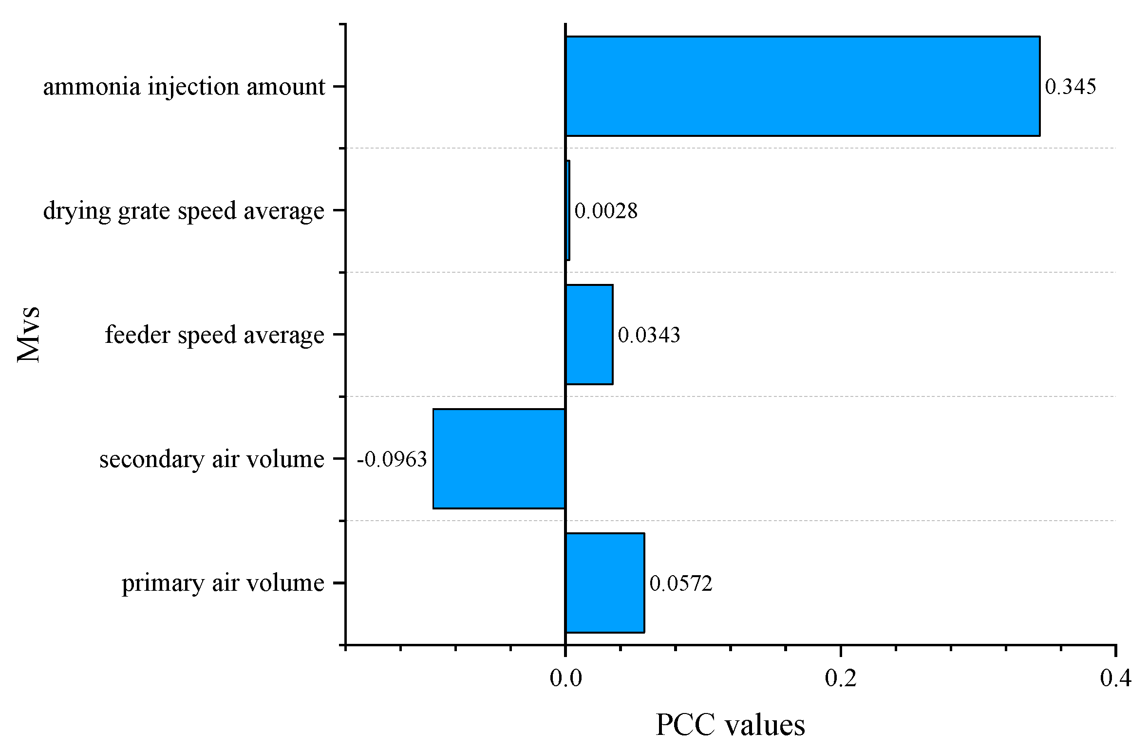
Figure 4.
Modeling strategy.
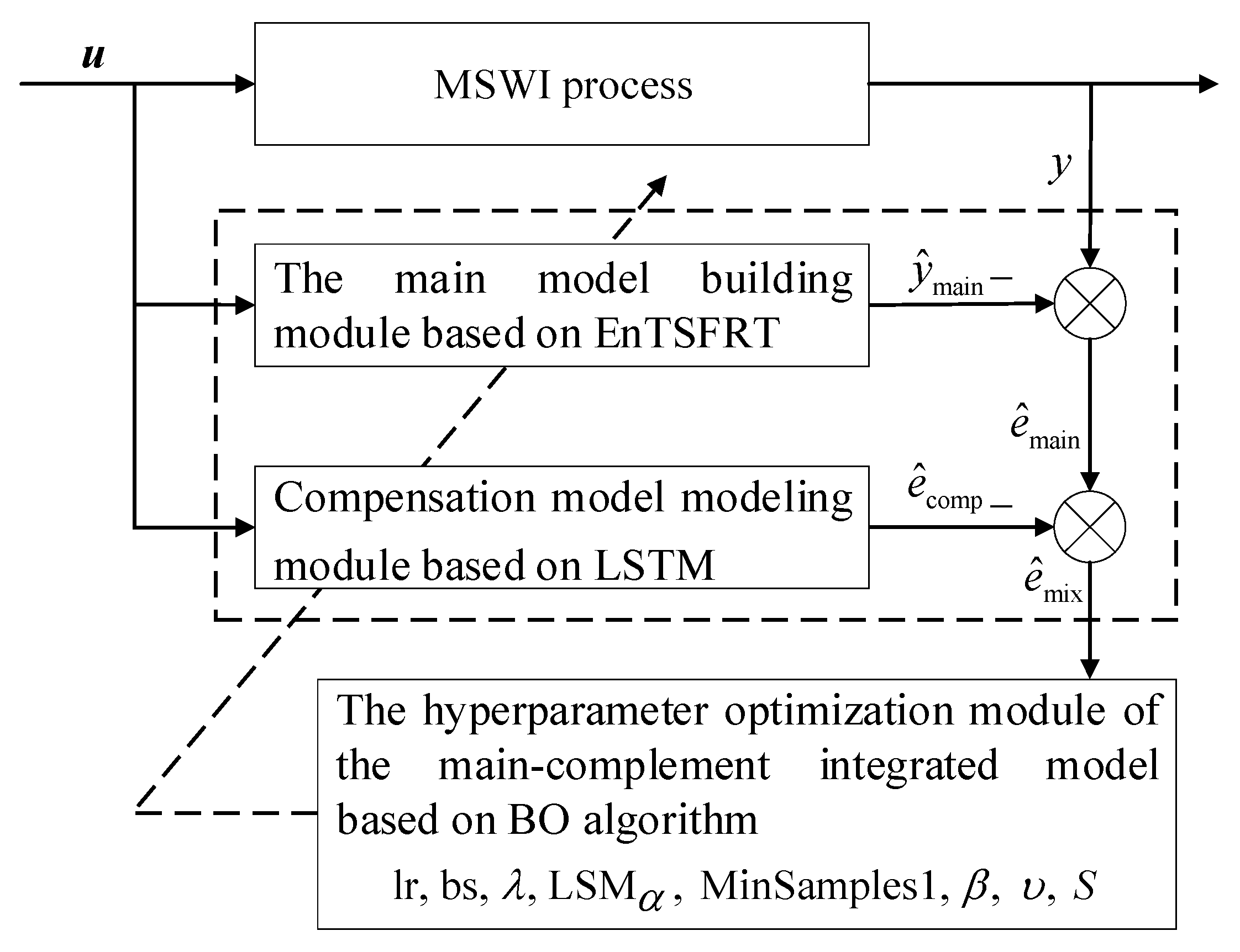
Figure 5.
Struct of main model construction module based on EnTSFRT.
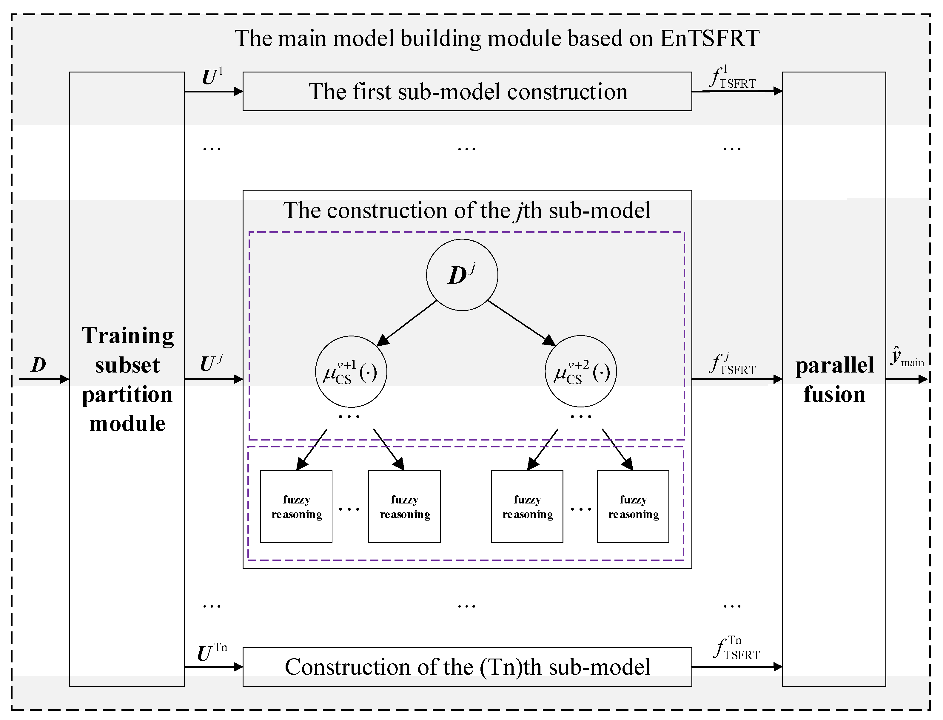
Figure 10.
Fitting curves of training set.
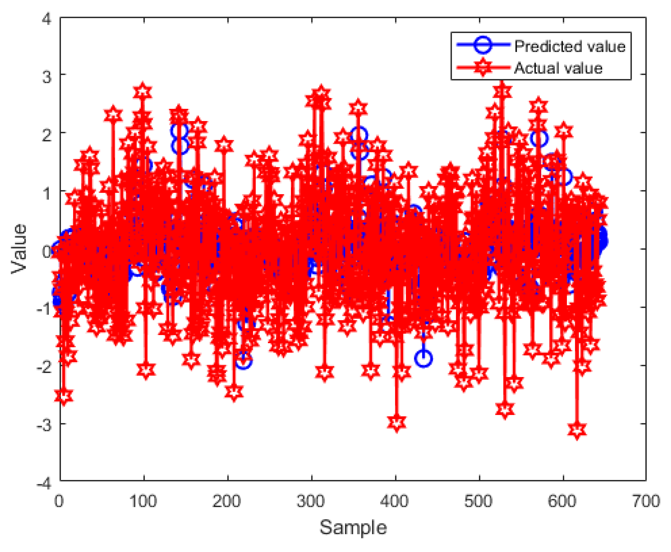
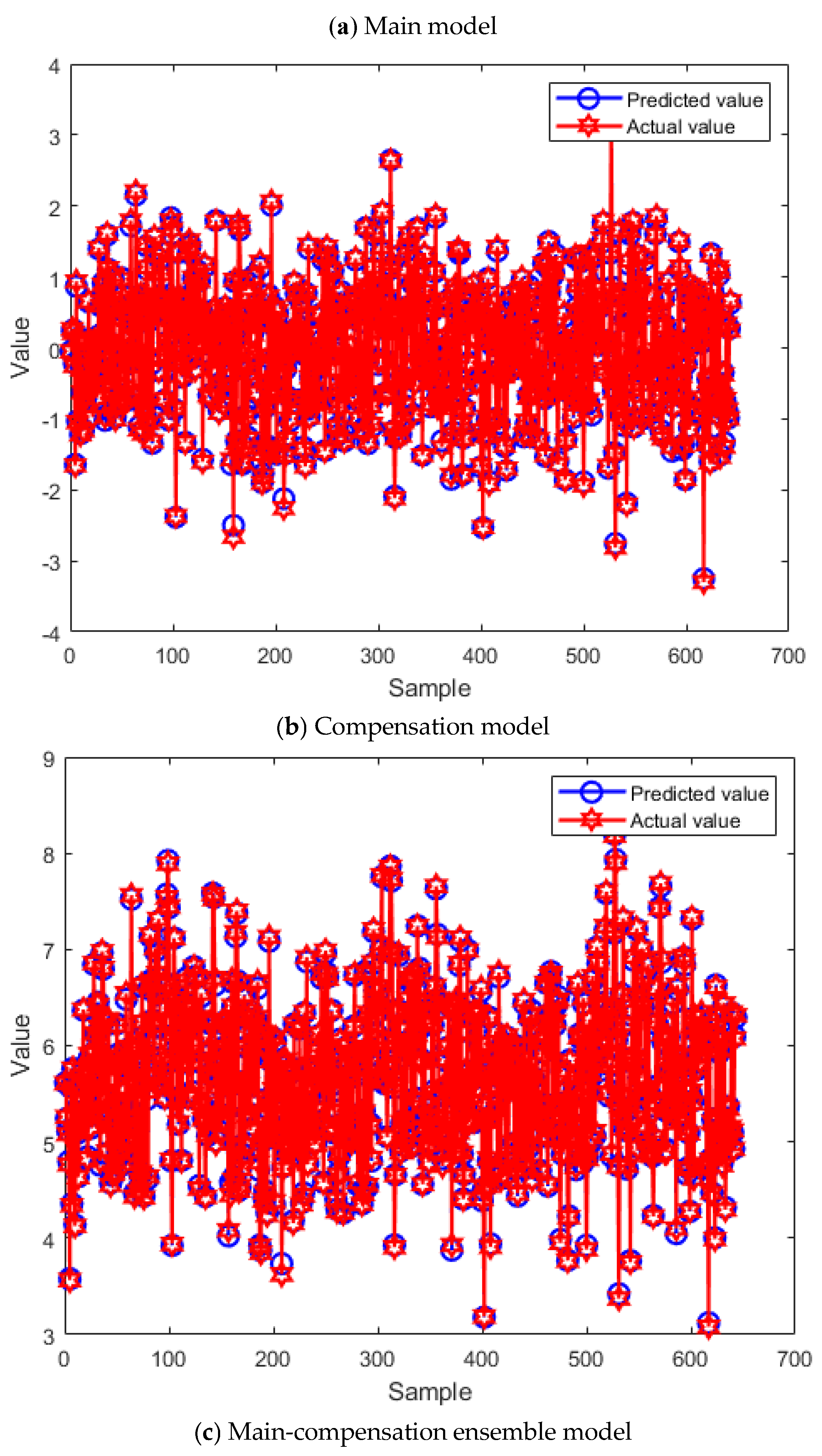
Figure 11.
The fitting curves of the testing set.(进行了修改).
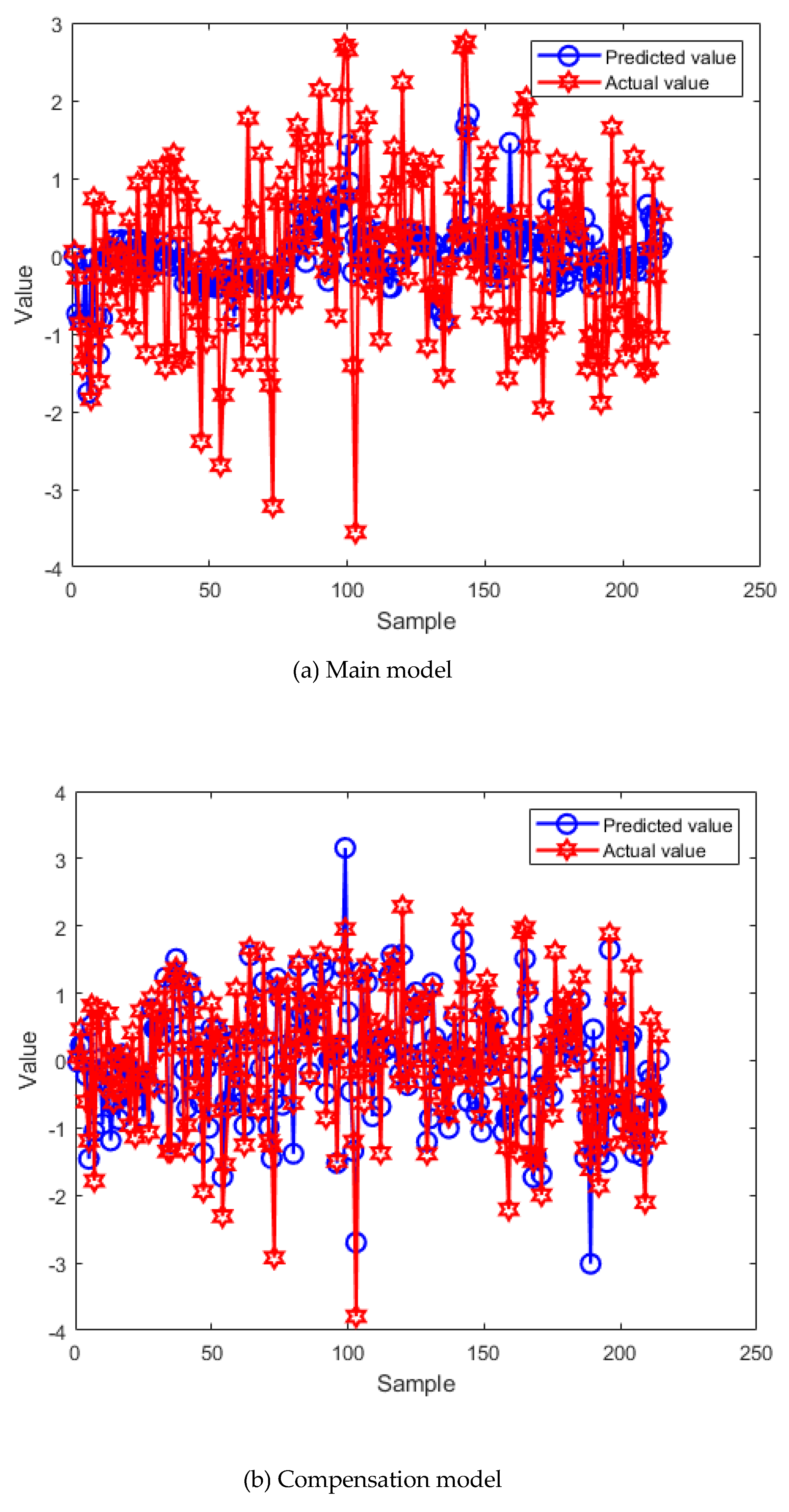
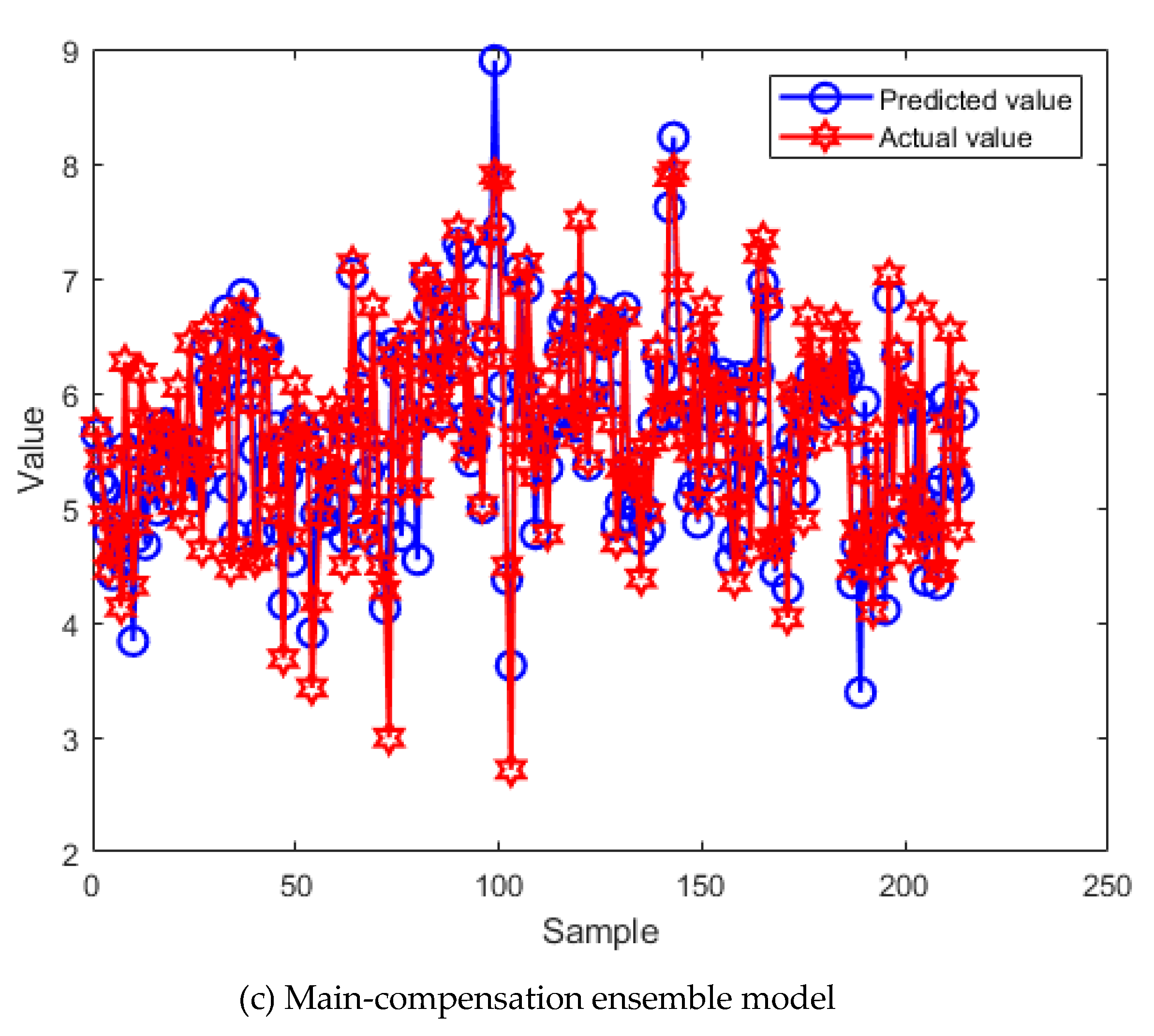
Figure 12.
Weight distribution diagram of the tree that constitutes EnTSFRT.
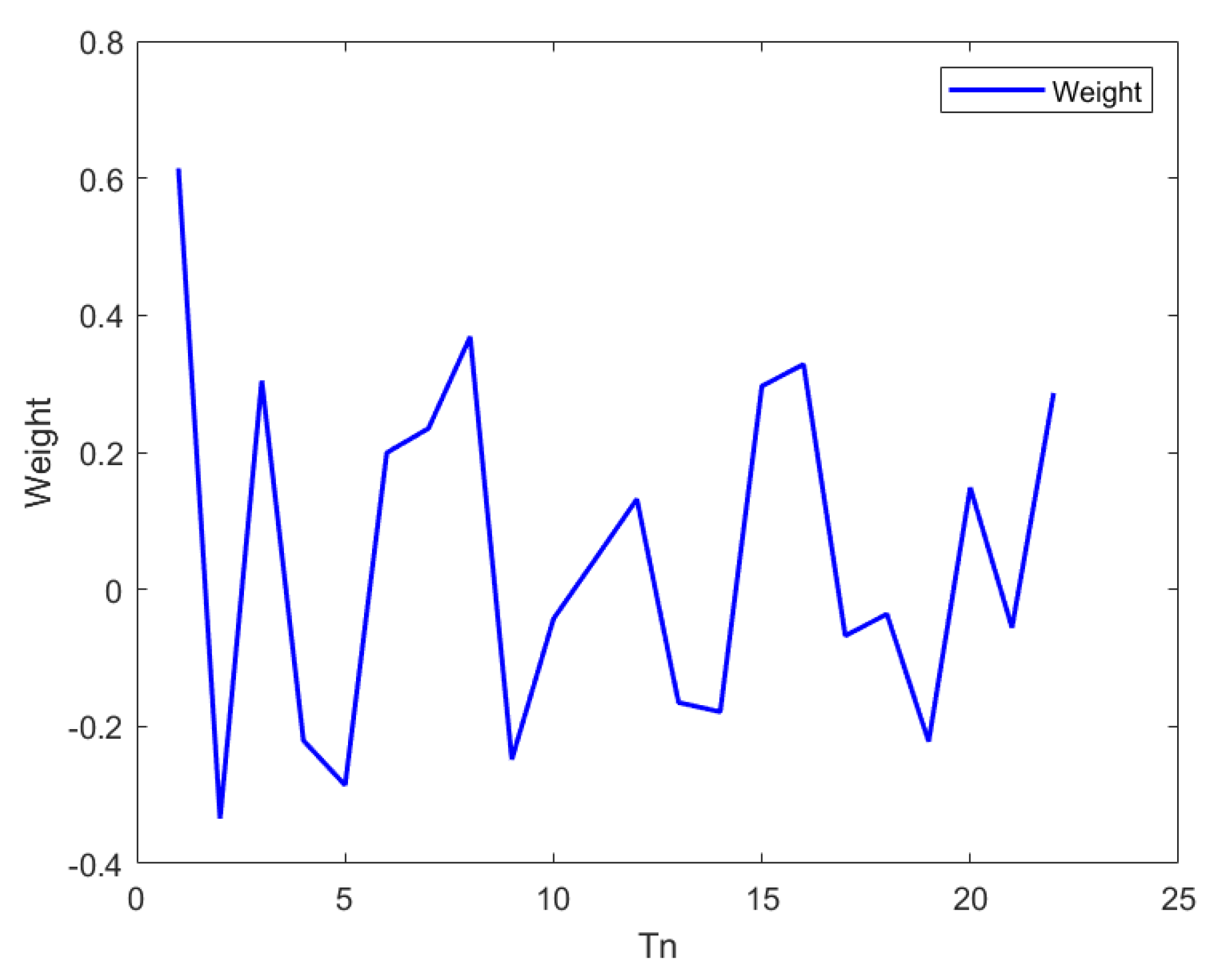
Figure 13.
The curve of the objective function in the BO optimization process.
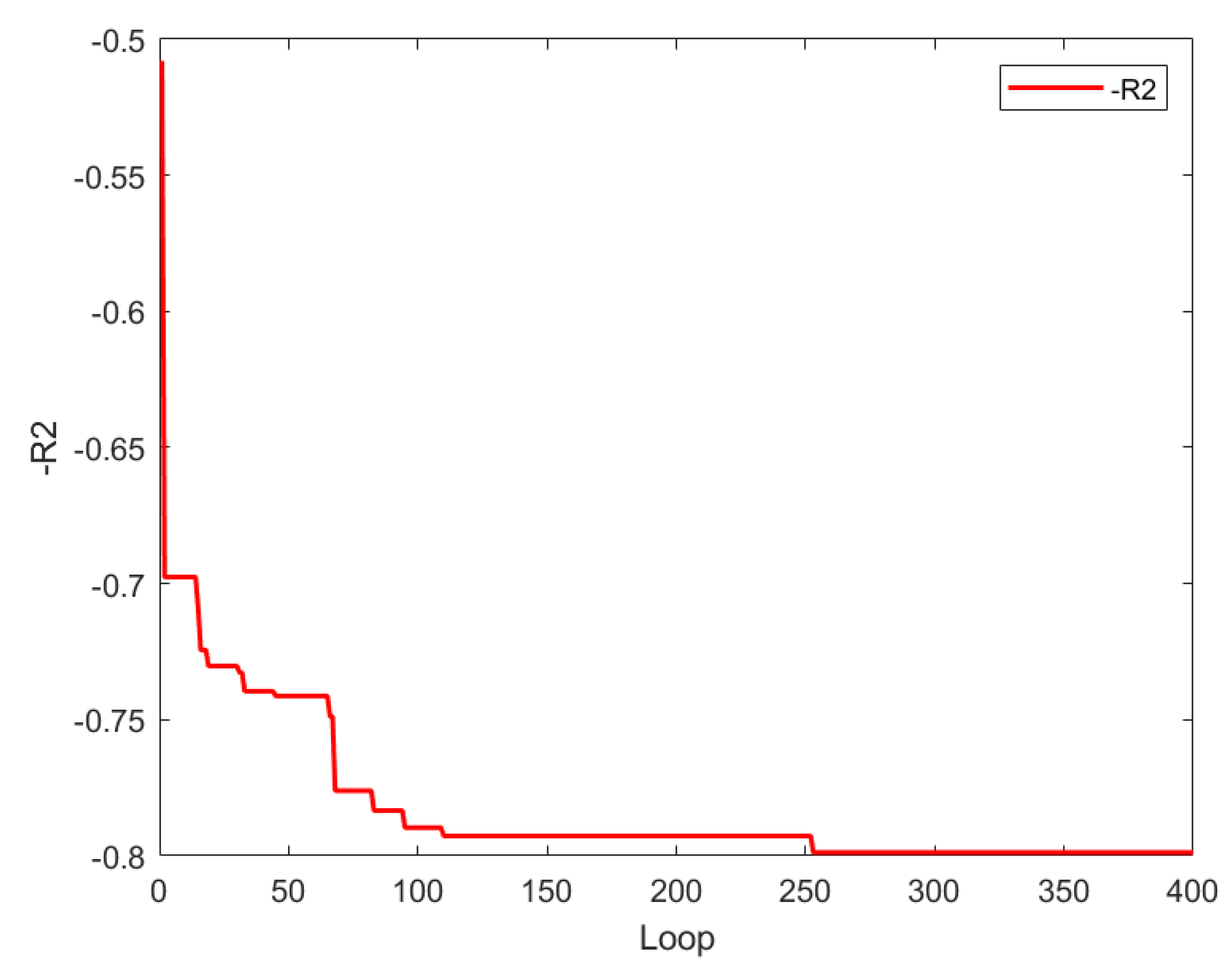
Figure 14.
The variation curves of the nine hyperparameters in the BO optimization process.
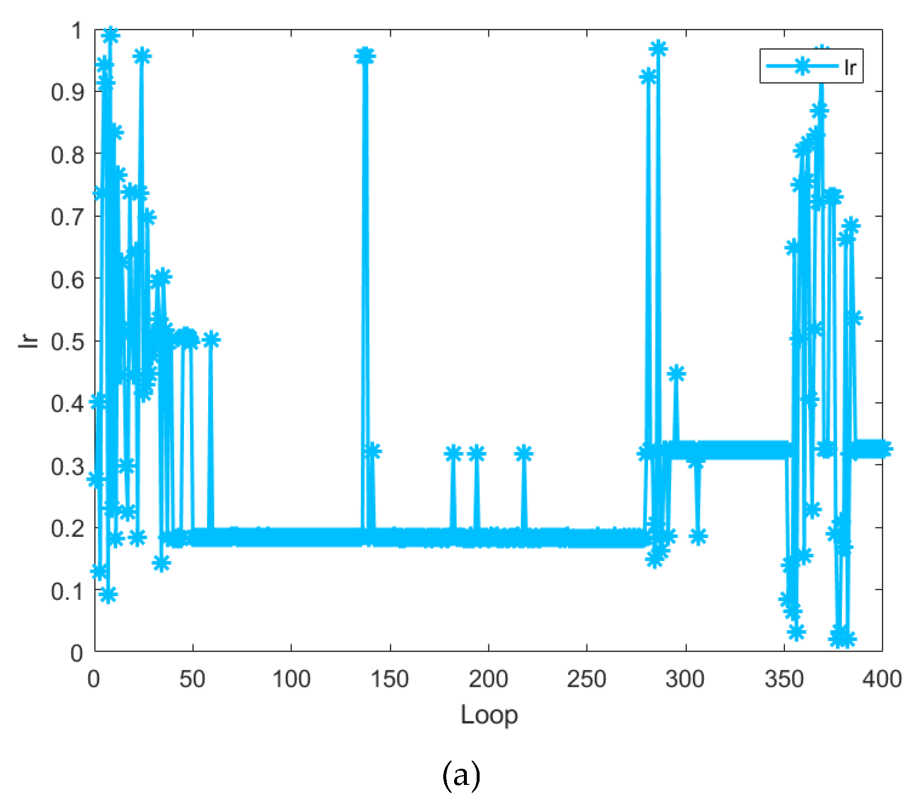
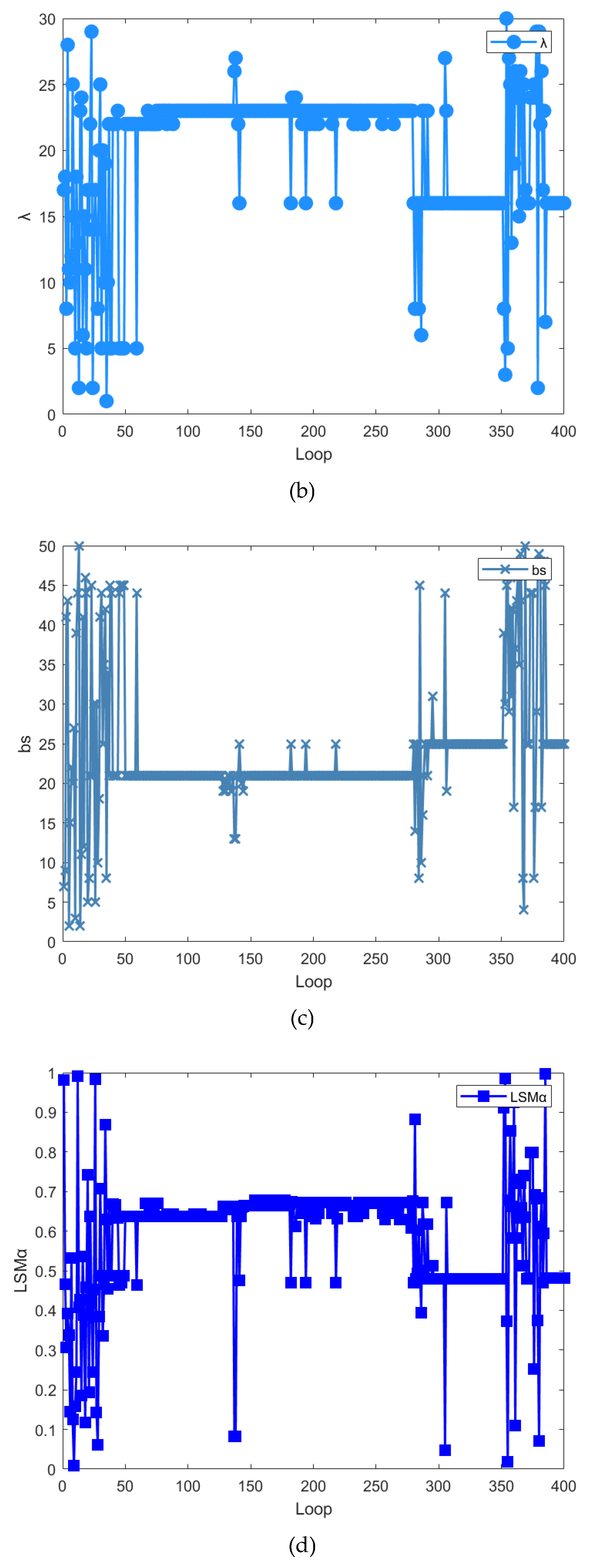
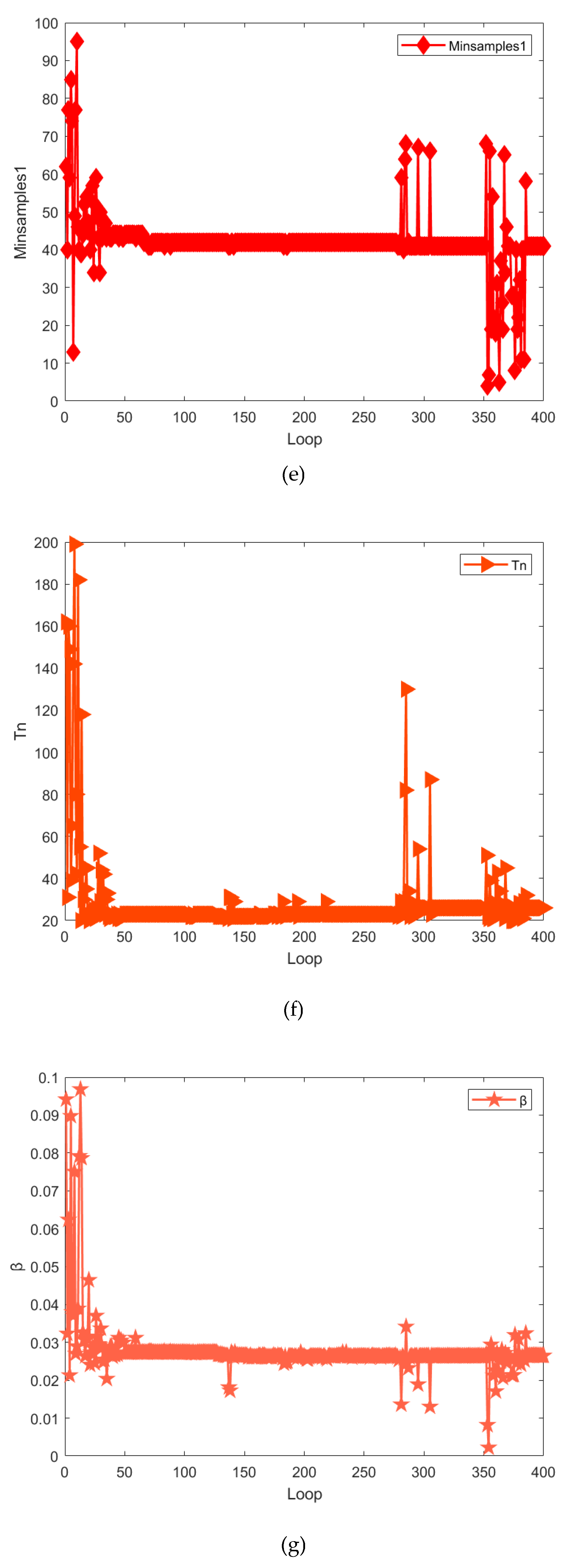
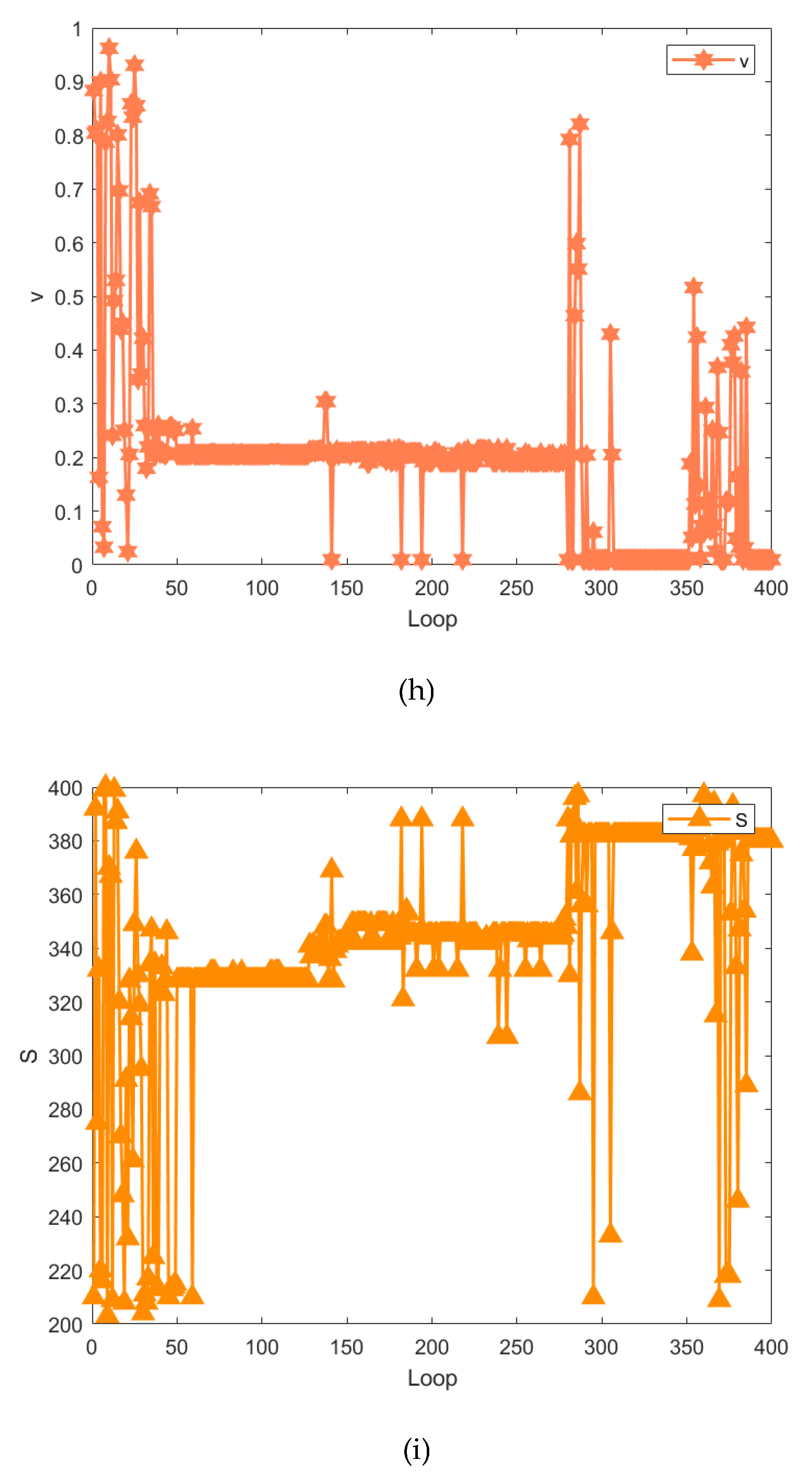
Figure 15.
Fitting curves of different methods on the testing set.
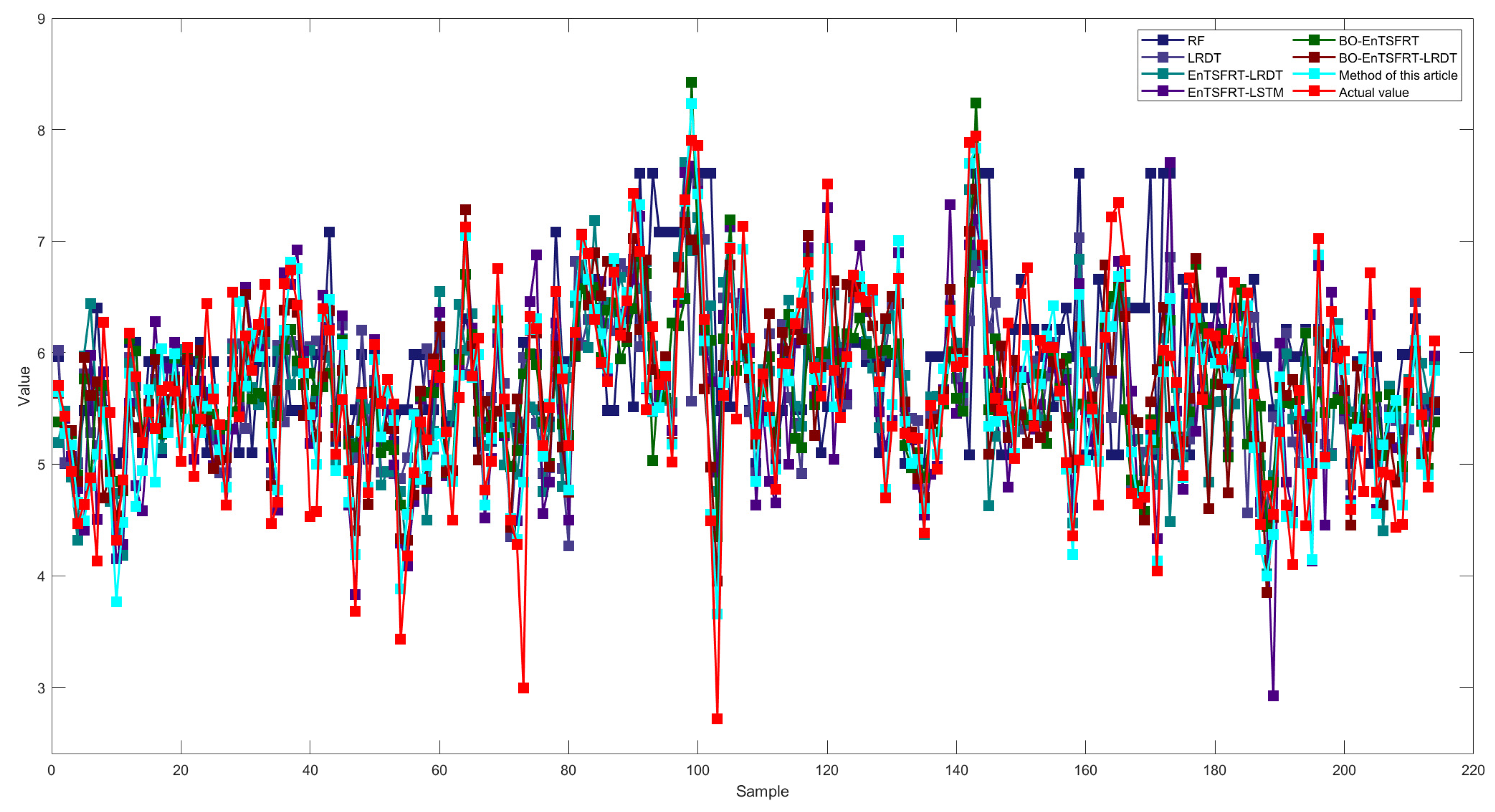
Figure 16.
The curve of hyperparameter sensitivity analysis in terms of average value of 20 times.
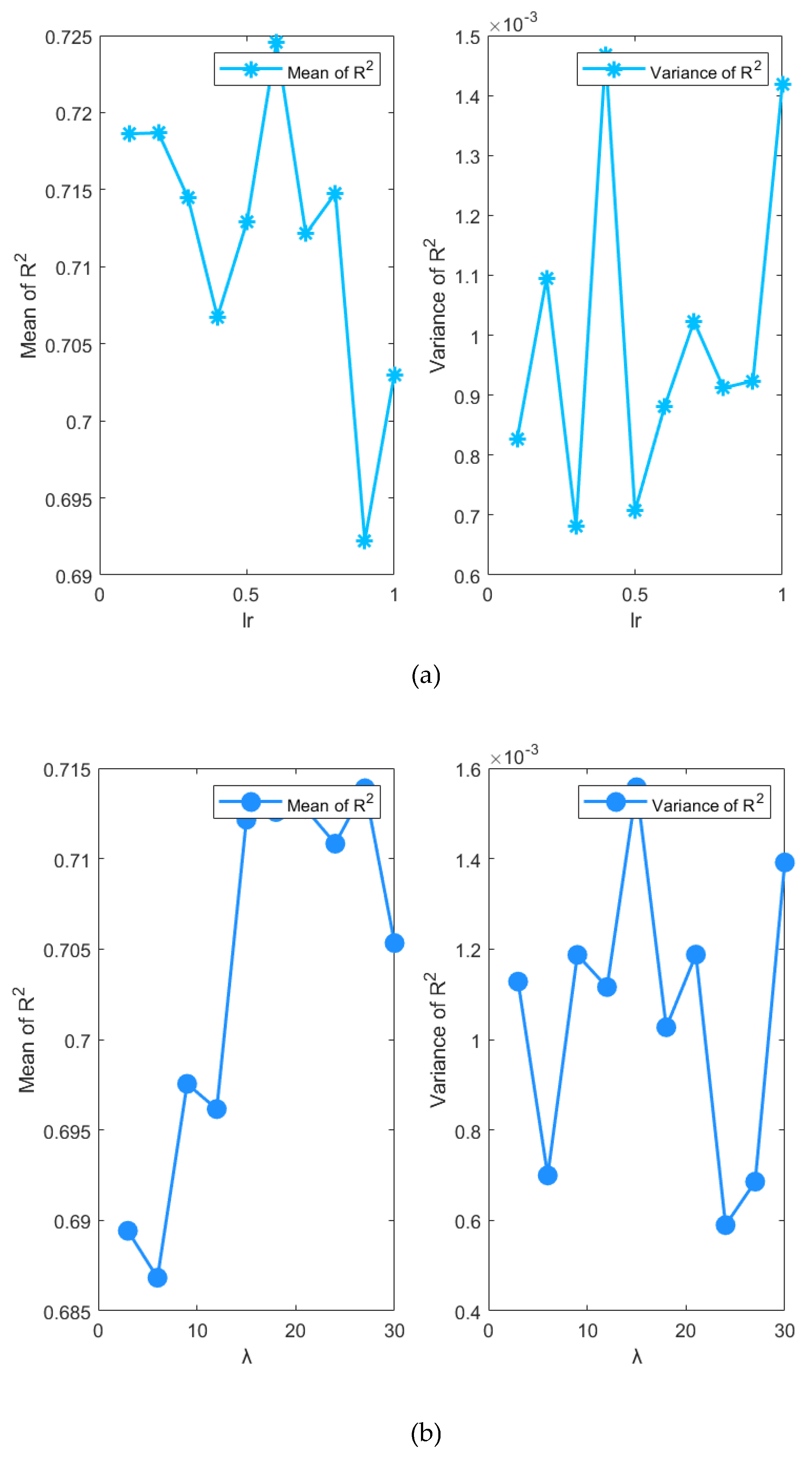
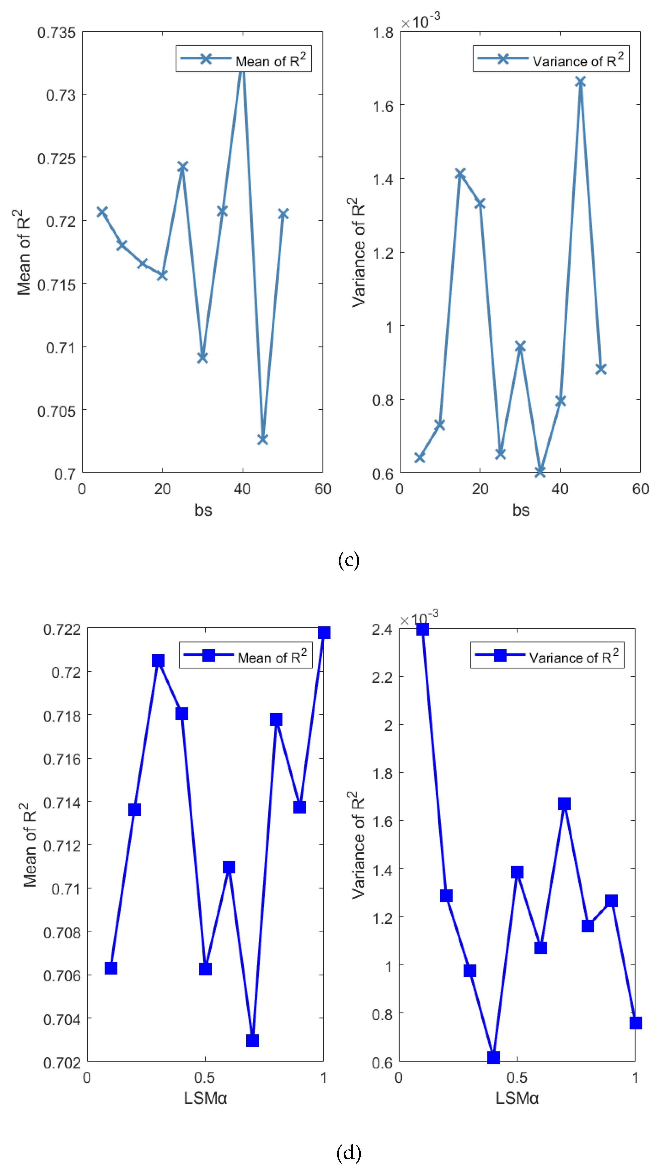
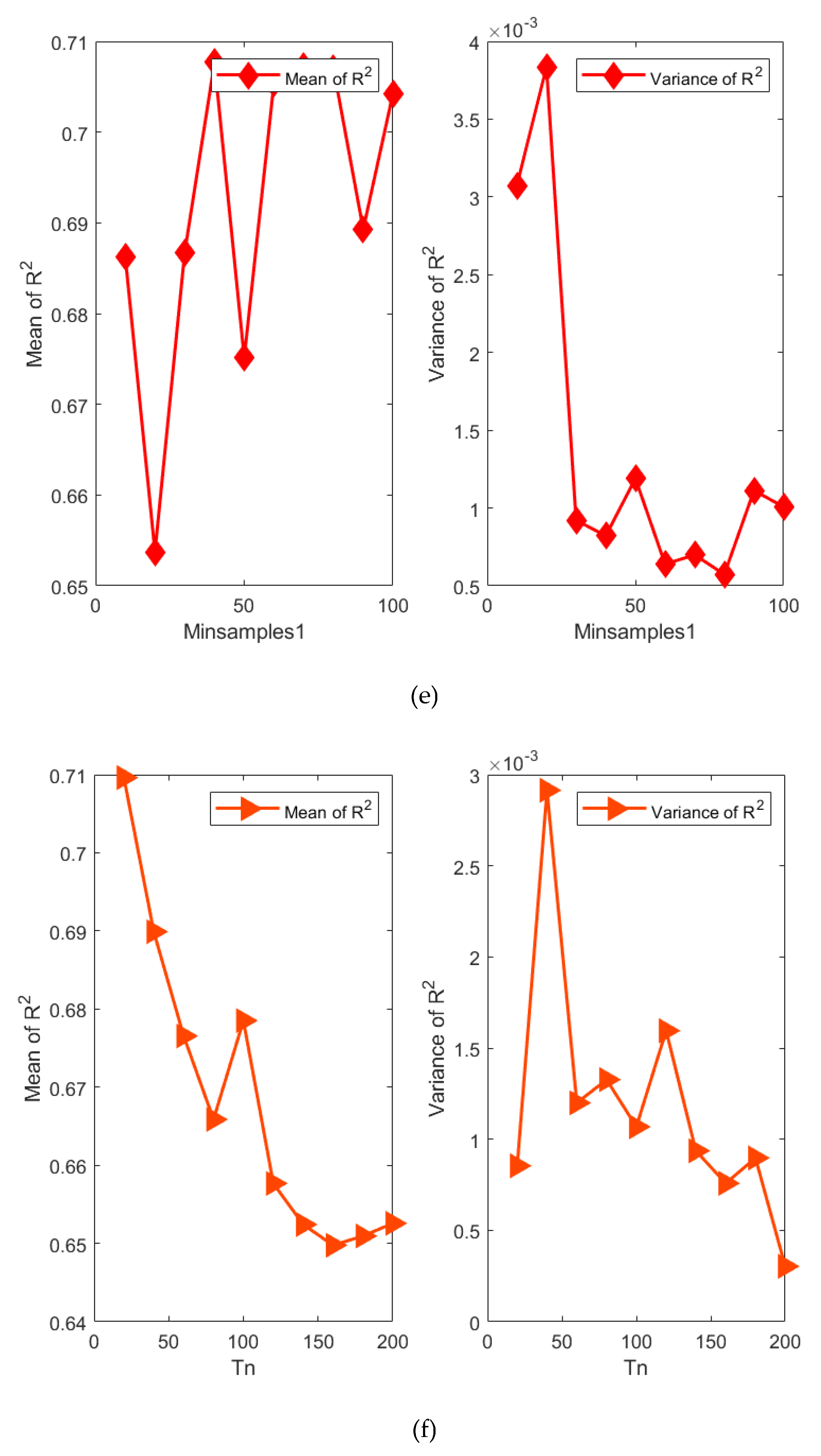
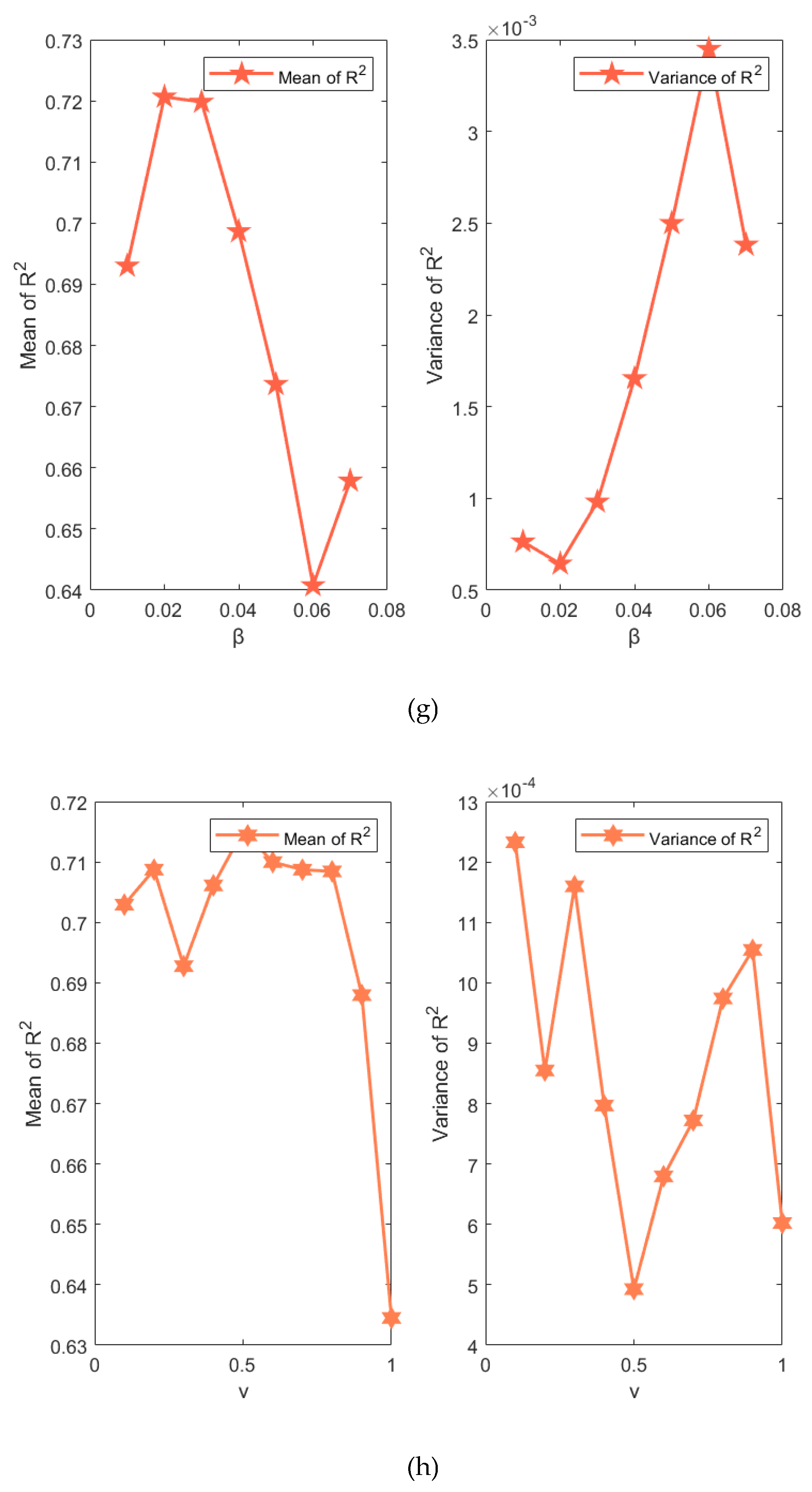
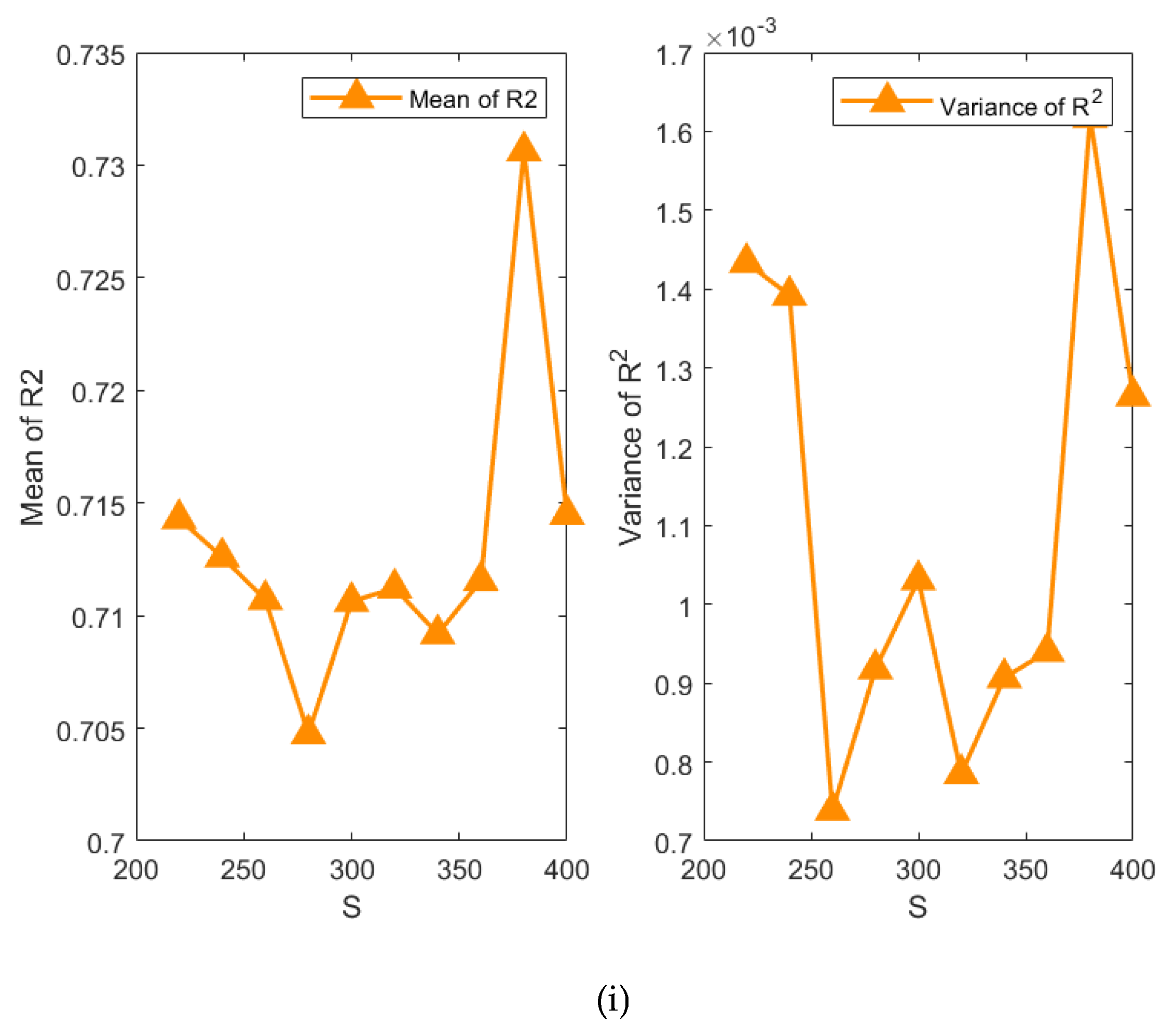
Table 1.
Pseudocode of BO-EnTSFRT-LSTM algorithm.
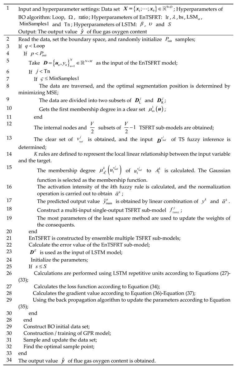 |
Table 2.
Statistical results of performance evaluation indexes of different methods.
| Dataset | Method | RMSE | MAE | R2 |
|---|---|---|---|---|
| Training set | RF | 8.6432E-01±1.1677E-31 | 6.4993E-01±1.2975E-32 | -8.8061E-02±8.1092E-34 |
| LRDT | 5.2664E-01±5.1899E-32 | 4.0872E-01±1.2975E-32 | 5.9604E-01±1.2975E-32 | |
| EnTSFRT-LRDT | 4.4932E-01±1.1640E-04 | 3.5266E-01±8.4882E-05 | 7.0088E-01±2.0645E-04 | |
| EnTSFRT-LSTM | 4.5666E-02±4.1522E-04 | 3.3945E-02±1.6713E-04 | 9.9639E-01±1.7202E-05 | |
| BO-EnTSFRT | 6.4563E-01±9.0752E-05 | 5.1347E-01±6.8136E-05 | 5.8308E-01±1.5481E-04 | |
| BO-EnTSFRT-LRDT | 4.3465E-01±2.9193E-32 | 3.4153E-01±1.2975E-32 | 7.2484E-01±5.1899E-32 | |
| BO-EnTSFRT-LSTM | 2.6610E-02±5.8122E-06 | 2.0684E-02±3.3649E-06 | 9.9896E-01±3.8281E-08 | |
| Testing set | RF | 9.7815E-01±5.1899E-32 | 7.4468E-01±5.1899E-32 | -2.0272E-01±1.2975E-32 |
| LRDT | 7.6825E-01±0.0000E+00 | 5.9607E-01±5.1899E-32 | 2.5808E-01±0.0000E+00 | |
| EnTSFRT-LRDT | 7.3435E-01±3.5825E-04 | 5.7583E-01±1.6158E-04 | 2.4216E-01±1.4912E-03 | |
| EnTSFRT-LSTM | 5.7702E-01±1.0583E-03 | 4.2354E-01±6.3545E-04 | 5.8020E-01±2.1789E-03 | |
| BO-EnTSFRT | 8.5004E-01±5.7774E-04 | 6.7746E-01±2.1606E-04 | 3.1419E-01±1.4888E-03 | |
| BO-EnTSFRT-LRDT | 6.4225E-01±1.2975E-32 | 4.9011E-01±5.1899E-32 | 4.8149E-01±2.9193E-32 | |
| BO-EnTSFRT-LSTM | 4.3991E-01±2.0766E-04 | 3.1771E-01±1.1515E-04 | 7.5649E-01±2.4804E-04 |
Table 3.
Interval setting of hyperparameters of the main-complement ensemble model.
| Model | Hyper Parameter | Range |
|---|---|---|
| Main Model | [0,1] | |
| [1, 30] | ||
| [1, 50] | ||
| [0, 1] | ||
| [1, 100] | ||
| [20, 200] | ||
| Compensation Model | [0, 0.1] | |
| [0, 1) | ||
| [200, 400] |
Disclaimer/Publisher’s Note: The statements, opinions and data contained in all publications are solely those of the individual author(s) and contributor(s) and not of MDPI and/or the editor(s). MDPI and/or the editor(s) disclaim responsibility for any injury to people or property resulting from any ideas, methods, instructions or products referred to in the content. |
© 2024 by the authors. Licensee MDPI, Basel, Switzerland. This article is an open access article distributed under the terms and conditions of the Creative Commons Attribution (CC BY) license (http://creativecommons.org/licenses/by/4.0/).
Copyright: This open access article is published under a Creative Commons CC BY 4.0 license, which permit the free download, distribution, and reuse, provided that the author and preprint are cited in any reuse.


