Submitted:
30 April 2025
Posted:
30 April 2025
You are already at the latest version
Abstract
In response to the increasing demand for reliable and robust artificial intelligence (AI) applications in petrochemical and process industries, this study proposes an intelligent prediction framework for estimating Research Octane Number (RON) loss during gasoline refining. The approach integrates a Sparse Autoencoder (SAE) for feature extraction and a Stacking Ensemble Learning (StackingEL) model for predictive regression, thereby enhancing performance in high-dimensional and noisy industrial datasets. Real-world process data obtained from a petrochemical enterprise were utilized for model training and evaluation. After comprehensive data preprocessing, the SAE effectively captured latent representations of complex process variables, which were then used to train twelve regression models including Lasso and advanced ensemble techniques. Experimental results indicate that the proposed SAE+StackingEL framework outperforms conventional methods in prediction accuracy, robustness, and generalization ability. This AI-assisted process modeling strategy contributes to optimizing gasoline production, reducing environmental emissions, and supporting cleaner and more sustainable industrial practices. The proposed method demonstrates significant potential for integration into Industry 4.0 systems and petrochemical process improvement.
Keywords:
gasoline refining
; Octane number prediction
; sparse autoencoder
; stacking ensemble learning
; Sustainable petrochemical processes
1. Introduction
In the context of increasing global attention to sustainability and environmental responsibility, the rapid rise in gasoline consumption and automobile usage has heightened the urgency of reducing pollutant emissions from the petrochemical industry [1]. Gasoline desulfurization—commonly referred to as gasoline cleaning—is an essential technological process aimed at lowering sulfur and olefin content while preserving the Research Octane Number (RON), which is critical to fuel performance [2]. However, during catalytic refining processes, particularly in units such as S-Zorb, RON loss is often an inevitable consequence, potentially leading to significant economic losses and reduced combustion efficiency [3].
For every unit of RON loss, refineries may suffer financial penalties of up to 150 CNY per ton, along with the associated increase in greenhouse gas emissions [4]. Therefore, accurately predicting octane number loss is not only vital for optimizing refinery operations and enhancing economic returns, but also for promoting cleaner production technologies, improving process sustainability, and aligning with global carbon neutrality goals. The S-Zorb process has been widely adopted across Chinese refineries due to its effectiveness in producing low-sulfur gasoline with relatively minimal RON loss [5,6,7,8]. However, this process is highly sensitive to a variety of operational and catalytic factors. The high dimensionality, non-linearity, and strong coupling among these parameters present challenges to real-time process control and predictive modeling [9,10,11,12]. In this regard, the integration of artificial intelligence (AI), especially in the form of trustworthy and robust learning frameworks, presents new opportunities for intelligent process monitoring, optimization, and decision-making in Industry 4.0 environments.
To address these challenges, this study proposes a hybrid AI-based prediction framework combining Sparse Autoencoder (SAE) for high-level feature extraction with Stacking Ensemble Learning (StackingEL) for robust regression modeling. The approach is applied to real operational data from a petrochemical refinery to accurately predict RON loss under varying production conditions. By capturing latent representations of complex influencing factors and fusing predictions from multiple base learners, the proposed method improves prediction accuracy, generalization, and robustness—enabling better process control, reducing unnecessary octane degradation, and supporting eco-friendly fuel production.
This paper is structured as follows: Section 1 outlines the research motivation and background; Section 2 provides a review of related works on data-driven modeling and AI in petrochemical process optimization; Section 3 details the theoretical basis of SAE and StackingEL; Section 4 introduces the proposed methodology and experimental design; Section 5 discusses the evaluation results; and Section 6 concludes with key findings and future directions.
2. Related Work
In recent years, researchers have explored a wide range of methods for predicting the Research Octane Number (RON) in gasoline, aiming to improve efficiency, reduce experimental overhead, and support process optimization in industrial settings. Traditional laboratory-based approaches typically rely on standardized octane testing engines that adhere to AMA or national regulatory protocols [13]. While these methods offer high accuracy, they are also associated with significant drawbacks, including high operational costs, time consumption, and the need for extensive manual testing. These limitations make them impractical for real-time monitoring or large-scale applications in modern refinery systems. In response, some studies have turned to analytical chemistry-based methods, which use gasoline composition and physical properties to predict RON. However, these techniques depend heavily on costly instrumentation and intricate experimental procedures, thus limiting their accessibility and scalability [14].
Beyond experimental techniques, mathematical modeling has also been employed to estimate octane values. Han et al. [15], for example, developed a regression-based model to predict RON using statistical principles. Other approaches, such as Partial Least Squares (PLS) regression [16], have shown some promise, but are limited in their ability to capture the nonlinear behavior and variable coupling that characterize complex refining operations. With the increasing availability of refinery process data, particularly through digital platforms such as Laboratory Information Management Systems (LIMS), data-driven modeling has become a practical and attractive alternative. Machine learning (ML) algorithms, including artificial neural networks (ANN), support vector machines (SVM), and random forests, have been applied to various predictive tasks in the petrochemical industry [17,18]. For instance, ANN models have been successfully used to correlate near-infrared spectral data with octane values, offering improved predictive accuracy and adaptability. Similarly, SVM models trained on molecular structure information have demonstrated high robustness and generalizability when validated with rigorous techniques such as leave-one-out cross-validation.
Recent studies further confirm the potential of ML models in gasoline quality prediction. A hybrid PCA-RFR model achieved R² = 0.983 with minimal prediction error (RMSE ≈ 3.22 × 10⁻⁴). Wu et al. [19] systematically compared SVM, ANN, and random forest models and found that random forest performed best in terms of overall predictive accuracy. In another study, Chen et al. [20] applied optimization methods that significantly reduced RON loss, with over 86% of cases achieving a 60–80% reduction rate. Despite these encouraging results, several limitations remain. Many single-model approaches struggle to handle the high dimensionality, complex interactions, and variability inherent in refinery operations. Moreover, traditional machine learning models often lack robustness and fail to generalize well under fluctuating process conditions.
To overcome these challenges, this study introduces a novel hybrid framework combining sparse autoencoder (SAE) for unsupervised feature extraction and stacking ensemble learning (StackingEL) for robust regression. SAE effectively captures latent variable representations and reduces dimensional complexity, while StackingEL enhances prediction performance by integrating the outputs of diverse base models. This dual approach provides greater adaptability and reliability, aligning with the goals of Industry 4.0 and sustainable process engineering by facilitating accurate, interpretable, and trustworthy predictions in real industrial environments.
3. Basic Theory
3.1. Sparse Autoencoder
An autoencoder is a type of neural network that employs a backpropagation algorithm to achieve output values that are equal to the input values. The network consists of an encoder and a decoder, as depicted in Figure 1. The encoder maps the input to a hidden representation, while the decoder attempts to reconstruct the original input by mapping this latent representation. The model's primary objective is to learn a function, hw,b(x) ≈ x, while obtaining a low-dimensional representation of the input data. The ultimate goal is to represent the original data in a smaller dimension with minimal loss of information, with the essential feature that the number of nodes in the input layer (excluding bias nodes) is equal to the number of nodes in the output layer, while the number of nodes in the hidden layer is less than the number of nodes in the input and output layers.
When the number of nodes in the hidden layer is large, even more than the number of nodes in the input layer, the self-coding algorithm can still be utilized, but with the addition of a sparsity restriction. This ensures that most of the nodes in the hidden layer are suppressed, and only a small portion is activated, thus achieving the same effect. This type of autoencoder is known as a sparse self-encoder. The data for the average activation of the sparse auto-coding hidden layer is represented as
In the formula, is the activation degree of the hidden neuron j when the input data is x. To make the mean activation near a relatively small value of p, the relative entropy of p and p is introduced as the penalty term, and the following loss function is obtained
3.2. Stacking Ensemble Learning
In the field of ensemble learning algorithms, stacking integration is a popular approach that utilizes a parallel learning method. It involves an untyped algorithm, known as the "primary learner," which is used to obtain the initial prediction values. These values are then optimized by a meta-learner to yield the final prediction results. In recent studies [21,22], a load prediction method was developed using a multimodel fusion stacking ensemble learning approach. This method employs long short-term memory (LSTM), gradient decision tree, random forest, and support vector machine as primary learners for ensemble learning. The prediction results of these primary learners are further refined by a meta-learner, allowing the method to fully utilize the strengths of each model and achieve accurate predictions for conventional loads.
Figure 2 illustrates the framework of stacking ensemble prediction, which comprises two layers of prediction models. The first layer, known as the base learner, uses raw data to generate initial prediction results. These results are then fed into the second layer, called the meta-learner, which optimizes the initial predictions to obtain the final prediction results. Overall, the stacking ensemble prediction method is an effective approach for improving the accuracy of load prediction models. The Stacking ensemble prediction method combines the advantages of different learners through the integration of multiple primary learners to make the prediction model with strong generalization ability; further, the meta-learner is used to optimize the output results of primary learners to improve the overall prediction accuracy [23].
In the model training process of stacking ensemble prediction, the k-fold cross-validation method is usually used for data partitioning and model training to reduce the risk of overfitting [24]. k-fold cross-validation process is shown in Figure 3. First, the original data set D is divided equally into k mutually exclusive subsets, D1, D2, ..., Dk. Then, the training and testing sets of the primary learner are constructed by selecting the concatenated set of k-1 of these subsets as the training set and the remaining 1 subset as the testing set, respectively. This way, k sets of training and testing sets can be obtained. For each primary learner in stacking ensemble prediction, k sets of training and testing sets are used to train and test the learner, and k test results S1, S2, ..., Sk are obtained. The process is called "cross-validation".
Based on the k-fold cross-validation method, the training data of the meta-learner can be further constructed. Assuming that there are T primary learners in the Stacking integration prediction, for the test set D, then i th fold, in the k-fold cross-validation,, there are T corresponding test result sets, respectively recorded as . After completing the house fold cross-validation, the dataset constitute the new sample set. Furthermore, is used as the input of the stacking integration prediction medium meta-learner, and serves as the output of the meta-learner.
When the k-fold cross-validation is completed, the training dataset of the meta-learner is obtained, where the input is recorded as and the output is recorded as . The above is the training process of the stacking integration prediction model based on the k-fold cross-validation method. Note that the effect of the k-fold cross-validation method depends largely on the value of k. The common values of k are 5,10,20, etc.
Although ensemble learning shows better performance than single machine learning methods [25]. It shows some problems, such as high computational complexity and low efficiency due to the diversity of types and rapid growth of data exhibited, and thus needs to be coupled with effective methods for feature extraction.
3.3. Optimized Selection of the Stacking Ensemble Prediction Learner
In the stacking ensemble prediction method, the selection of base learners is critical for achieving accurate and generalizable predictions. To enhance diversity and avoid redundancy, the selected primary learners should be "accurate yet heterogeneous," meaning they must not only exhibit strong predictive capability but also be constructed from fundamentally different learning paradigms. This diversity enables the ensemble to learn a richer set of patterns and reduces overfitting risks. Accordingly, this study evaluates the predictive performance and variance contribution of several representative algorithms and selects the following models as base learners: Lasso Regression, Ridge Regression, Support Vector Regression (SVR), Elastic Net Regression (ELA), Naive Bayes (NB), Logistic Regression (LR), Random Forest (RF), Gradient Boosting Regression (GBR), Extremely Randomized Trees (ERT), and Extreme Gradient Boosting (XGB) [26,27].
To aggregate the outputs of the base learners, this study adopts the Least Squares Support Vector Machine (LSSVM) as the meta-learner. Owing to its robustness in handling large-scale, high-dimensional, and nonlinear datasets, LSSVM offers notable advantages for optimizing the overall prediction performance of the ensemble [28,29].
4. Framework
This paper proposes that the framework of the RON loss prediction method is based on the sparse autoencoder and the stacking ensemble learning method, which is shown in Figure 4.
The main steps are as follows.
(1) Data collection, obtaining data related to plant operation and gasoline properties through the petrochemical enterprise database.
(2) Data preprocessing, including format unification, missing number processing, outlier processing, and data normalization.
(3) Feature parameter dimensionality reduction, using sparse self-encoder to reduce the dimensionality of the feature parameters.
(4) Model training and prediction, using the reduced-dimensional data set as input, multiple initial learners are trained and tested, and the algorithms with better prediction results are ensemble into the stacking ensemble learning framework for further training and prediction.
(5) Result evaluation using Evs, Meanae, Mse, Medianae, and R2 evaluation parameters to evaluate the prediction results from different perspectives.
4.1. Data Set
The original dataset used in this study was sourced from the PHD real-time database and the LIMS experimental database of a catalytic cracking gasoline refining and desulfurization unit operated by a petrochemical company. Information related to feedstocks, products, and catalysts was retrieved from the PHD and LIMS systems at a sampling frequency of twice per week. To ensure sufficient data volume and experimental reliability, LIMS data were collected across two time periods: from April 2017 to September 2019 and from October 2019 to May 2020, covering a total duration of approximately three years. Operational variables were obtained from the PHD system. During the first data collection period, sampling occurred every 3 minutes, while in the second period, the frequency was every 6 minutes. The raw dataset comprises 7 feedstock property variables, 2 adsorbent generation property variables, 2 regenerated adsorbent property variables, 2 product quality variables, as well as several uncontrollable process variables. In total, 354 operational variables were recorded, leading to a dataset containing 367 variables overall. To streamline preprocessing and analysis, all data entries were sorted in descending order based on their time stamps.
4.2. Data Preprocessing
The raw data were preprocessed as below:
(1) Uniform data format. The second field is timestand type, not float type, so this column is deleted directly.
(2) Missing data filling. Delete the columns with missing data greater than 20%, and for the columns with missing data less than 20%, use the average of the data before and after 2h to fill in.
(3) Outlier processing. The outliers are removed according to the Lajda criterion (3 criterion).
criterion: Let the measured variables be measured with equal precision to obtain ,and calculate their arithmetic mean and residual error and the standard error is calculated according to the Bessel formula. If the residual error of a measurement , satisfying is a bad value containing coarse error values and should be rejected. The Bessel formula is shown in equation 5-1-1.
4.3. Parameters Dimension Reduction
The feature parameters were dimension-reduced using SAE. SAE sets different numbers of neurons in the hidden layer to obtain the dimension of extracted features corresponding to the number of neurons in the hidden layer. The feature expression of different dimensions may cause significant differences in the effect of anomaly detection. To determine the appropriate feature dimension, which can ensure the loss of input information within a controlled range while minimizing the number of feature parameters, several experiments were conducted. The feature dimension hiddensize was selected in the interval {10-100}, and other parameters, including the number of iterations, epochs, learning rate, training data batchsize, etc., were fine-tuned using grid search.
Figure 5 shows the decoded reconstruction and the information loss on the original data at different feature dimensions. It can be observed that when the feature dimension is 31, the information loss is only 0.9% at the inflection point of the change curve. Therefore, this number was chosen as the feature parameter dimension after dimension reduction. In this paper, the 367 variables were finally encoded into 31 deep features.
4.4. Model Training and Prediction
To demonstrate the rationale behind selecting the stacking ensemble prediction primary learner process, this section initially analyzes the prediction performance and variability of various single models. Specifically, Lasso regression, Ridge Regression (Ridge), Support Vector Regression (SVR), Elastic Net Regression (Ela), Naive Bayes (NB), Logistic Regression (LR), Random Forest (RF), Gradient Boosting Regression (GBR), Extremely Randomized Trees (ERT), and Extreme Gradient Boosting (XGB) are selected as the candidate options for the primary learner.
Experiments were designed to compare the prediction results of each primary learner individually. The four primary learners with good performance were selected to be ensemble into the stacking learning process. The prediction results of these four primary learners are used as inputs to be ensemble into the secondary learners, and the final prediction results are then generated.
4.5. Evaluation
Scoring measures to assess the effect of the regression model. There are many criteria for the applicability of the model. This paper uses Explained variance score (Evs), Mean absolute error (Meanae), Mean squared error (Mse) and R2 determination coefficient (R2) between the actual calculated value and the model estimated value.
(1)Explained Variance Score
y: predicted value, y: true value, Var: variance. This indicator is used to measure how well our model explains the fluctuations of the data set. If the value is 1, the model is perfect, and the smaller, the worse the effect is.
(2)Mean Absolute Error
y: predicted value, y: true value. Given the average absolute error of a data point, the smaller the value, the better the model fits.
(3)Mean Squared Error
y: the predicted value, then y: the true value. This is a common method in mathematical statistics.
(4)Median Absolute Error
y: the predicted value, the y: the true value, and the median absolute error applies to the measure of the data containing the outliers.
(5)R2 Coefficient of Determination
The proportion that can be explained by the estimated multiple regression equation measures the interpretation of the variation of the dependent variable. The value is between 0 and 1. The closer the value is to 1, the higher the interpretation of the variable. The closer the value is to 0, the weaker the interpretation is. Generally speaking, by increasing the number of independent variables, the regression square sum increases, and the residual square sum will decrease, so R2 increases; otherwise, by reducing the number of independent variables, the regression square sum decreases, and the residual square sum increases.
5. Results and Discussion
5.1. Analysis of the Predictive Results from a Single Model
The evaluation metrics of each individual prediction model are summarized in Table 1. As observed, the Elastic Net Regression (ELA), Random Forest (RF), and Gradient Boosting Regression (GBR) models exhibit relatively high prediction accuracy. The Ridge Regression model demonstrates similar predictive performance to the Support Vector Regression (SVR) model. However, in comparison to SVR, the Ridge model achieves Evaluation Score (Evs) and R² values that are closer to 1, while its Mean Absolute Error (Meanae), Mean Squared Error (Mse), and Median Absolute Error (Medianae) are lower and closer to 0. These results suggest that the Ridge model exhibits greater stability and robustness. To sum up, the ELA, RF, GBR, and Ridge models were selected as the base learners in the proposed stacking ensemble framework, with the Least Squares Support Vector Machine (LSSVM) model serving as the meta-learner.
5.2. Analysis of the Predictive Results of the Stacking Ensemble Learning Model
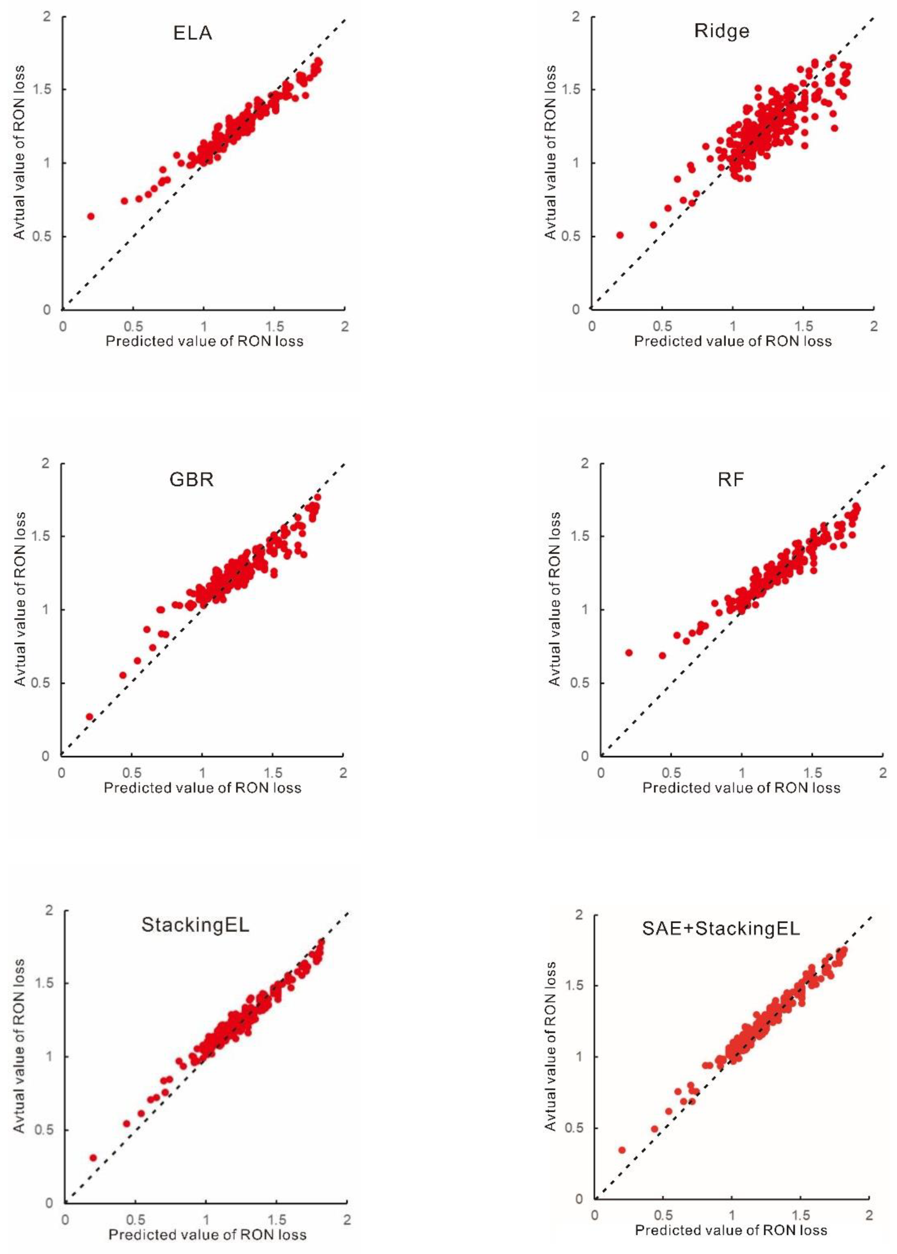
Using the reduced dataset (processed by SAE) as input, RON loss predictions were conducted using the StackingEL model. The predictive performance was then compared with the best-performing single prediction models, as shown in Table 1. The results demonstrate that both the StackingEL and SAE+StackingEL models outperform individual models in terms of predictive accuracy. Notably, the SAE+StackingEL model achieved the highest overall performance. It produced an Explained Variance Score (EVS) closest to 1, indicating near-perfect prediction ability; the smallest Mean Absolute Error (Meanae), indicating the best fit to the data; and an R² value closest to 1, showing the highest degree of explained variability.
In summary, the SAE+StackingEL model demonstrates superior generalization and robustness, delivering more accurate and reliable predictions. As illustrated in Figure 6, all fitted models show high accuracy within acceptable error ranges, with the SAE+StackingEL model achieving the best performance—particularly in predicting extreme or boundary values.
In addition, a visual analysis of the R² values is presented below. Combined with the results in Table 1 and Figure 6, it is evident that the SAE+StackingEL model achieves the lowest overall error metrics among all methods, with a fitting performance that closely approximates the actual values. The use of multiple randomized cross-validations during the experiments further contributes to the stability and robustness of the model, as it results in minimal variation in octane loss predictions. The StackingEL model, while slightly less accurate than SAE+StackingEL, also exhibits error metrics within an acceptable range. Its predictions converge toward the optimized regression surface where most sample points are concentrated, indicating strong predictive consistency. In conclusion, the StackingEL method effectively improves the accuracy of RON loss prediction, and the integration of SAE further enhances the model’s fitting performance and generalization ability.
Figure 7.
Scatter diagram comparison of models.
6. Conclusion
This study presents a novel RON loss prediction framework that integrates Sparse Autoencoder (SAE) with Stacking Ensemble Learning (StackingEL), aiming to enhance prediction accuracy and capture complex variable interactions within petrochemical refining processes. The method addresses critical industrial needs by introducing a scalable, robust, and interpretable model architecture suited for real-time data-driven applications in refining operations.
By leveraging the unsupervised learning capabilities of SAE for deep feature extraction and dimensionality reduction, followed by ensemble learning with Ridge, Elastic Net, Random Forest, and Gradient Boosting as base models, the proposed approach significantly outperforms traditional single-machine learning models in both accuracy and robustness. The results demonstrate not only reliable forecasting of RON loss but also improved adaptability to operational fluctuations, aligning with Industry 4.0 paradigms. From a technological perspective, this work offers a modified and intelligent solution tailored to modern petrochemical processes. The model supports sustainable process optimization by minimizing octane loss and enabling cleaner fuel production, thus contributing to reduced pollutant emissions. This aligns with circular economy principles and environmental compliance goals.
In summary, the integration of advanced machine learning with industrial process intelligence offers a promising path for improving the environmental and operational efficiency of the chemical industry. The proposed framework holds broad applicability for sustainable and intelligent transformation in other process industries.
Supplementary Materials
The supplementary materials include additional figures, tables, and detailed model parameters that support the findings of this study. These materials are available upon request or can be accessed in the online version of the article.
Author Contributions
All authors contributed to the study's conception and design. Shitao Yin and Xiang Li conducted data cleaning and analysis. Xiaochun Lin and Shitao Yin developed the framework and performed the experiments. Xiaochun Lin interpreted the results and drafted the manuscript. All authors reviewed and approved the final manuscript.
Funding
This study was funded by Construction and Application of Information Management System for Geological Experimental Testing, Geological Survey Project, China Geological Survey (DD202510013).
Data Availability Statement
The datasets used in the current study are available from the author on reasonable request.
Acknowledgments
This work was supported by the Geological Survey Project of China (Project No. DD202510013), and the authors would like to express their sincere gratitude to the Key Laboratory of Eco-Geochemistry, and National Research Center for Geoanalysis for their valuable assistance.
Conflicts of Interest
The authors declare that they have no known competing financial interests or personal relationships that could have appeared to influence the work reported in this paper.
References
- Zhang Chao, Xia, Chun, Fang Junhua, et al. Influence of gasoline aromatic hydrocarbon content on particulate matter emission and its microphysical and chemical properties. Internal Combustion En-gine Engineering 2018, 39, 8–14. [Google Scholar]
- Zhu Xiao, Jiang Juncheng, Pan Yong, et al. Research on the prediction of octane number of alkanes based on molecular structure. Industrial Safety and Environmental Protection 2011, 37, 27–29. [Google Scholar]
- Lucimar V A, Nathalia D S A S, Vinicius R, et al. Effects of gasoline composition on engine performance, exhaust gases and operational costs. Renewable and Sustainable Energy Reviews 2021, 135, 110196. [Google Scholar] [CrossRef]
- Kelly J, Barlow C, Callis J. Prediction of gasoline octane numbers from near-infrared spectral features in the range 660—1215 nm. Anal Chem 1989, 61313–61320.
- Yu Fan, Fan Baoan, Huang Tiegai.Research progress of data mining in chemistry and chemical engineering[J]. Applied Chemical Industry, 2017, 46(1): 159-162, 166.
- Xu Xiao, Zhao Hongtao, Lu Kailiang, et al. BDMOS: Big data mining optimization system and its application in chemical process optimization. Computers and Applied Chemistry 2018, 35, 433–439. [Google Scholar]
- Tian Jingzhi, Du Xiaoxin, Zheng Yongjie, et al. Prediction of sulfur content in hydrodesulfurization diesel oil based on the PSO-BP neural network. Petrochemical Engineering 2017, 46, 62–67. [Google Scholar]
- Xu Zhanghua, Huang, Xuying, Lin Lu, et al. BP neural networks and random forest models to detect damage by Dendrolimus punctatus Walker. Journal of Forestry Research 2020, 31, 107–121. [Google Scholar] [CrossRef]
- Wang Wei, Wang, Kun, Yang Fan, et al. Construction and analysis of gasoline yield prediction model for fluid catalytic cracking unit (FCCU)based on GBDT and P-GBDT algorithm. Acta Petrolei Sinica (Petroleum Processing Section) 2020, 36.
- Qiu Aibo, Zhou Rujin, Qiu Songshan, et al. Research the progress of gasoline components and gasoline octane number prediction methods. Natural Gas Chemical Industry 2014, 39, 62–66. [Google Scholar]
- Kardamakis A, Pasadakis N. Autoregressive modeling of near-R spectra and MLR to predict RON values of gasoline. Fuel 2010, 89, 158–161. [Google Scholar] [CrossRef]
- Soo H P, Hong Y, Mubarakat S, et al. Detection of apple Marssonina blotch with PLSR, PCA, and LDA using outdoor hyperspectral imaging. Spectroscopy and Spectral Analysis 2020, 40, 1309–1314. [Google Scholar]
- Deng Chengxin, Xu, Jinlong, Zou Lianning, et al. Application and prospects of near infrared spectroscopy in crude oil analysis. In-spection and Quarantine 2019, 29, 128–131. [Google Scholar]
- Ghosh P, Hickeyk J, Jaffe S. Development of a detailed gasoline composition-based octane model. Industrial & Engineering Chemistry Research 2006, 45, 337–345. [Google Scholar]
- Han Zhiqi. National methanol vehicle pilot methanol gasoline co-lane number test research[D]. Xi'an: Chang'an University, 2015.
- Qiu Aibo, Zhou Rujin, Qiu Songshan, et al. Research progress of gasoline components and gasoline octane number prediction methods. Natural Gas Chemical Industry 2014, 39, 62–66. [Google Scholar]
- Zhang Baoquan, Ma Yali, Guan Rui, et al. A neural network method that can give the reliability of oil chromatographic fault diagnosis of oil-filled electrical equipment. Science Technology and Engineering 2021, 21, 1857–1864. [Google Scholar]
- Qin Yucui. Quantitative structure of organic mixture based on artifi-cial neural network research on the relationship of nature[D]. Xi'an:Xi'an Shiyou University, 2018.
- Wu Ping, Zhong Yihua, Yong Xue, et al. Application of data mining method in calculating the loss of gasoline octane number. Science Technology and Engineering 2022, 22, 4046–4054. [Google Scholar]
- Chen Yanzhan, Hu Hao, Ren Zichang, et al. Model Analysis of Gasoline Octane Loss in Catalytic Cracking Post Refining Unit Based on XG Boost and Improved Gray Wolf Optimization A lgorithm. Acta Petrolei Sinica(Petroleum Processing Section) 2022, 38, 208–219. [Google Scholar] [CrossRef]
- Shi Jiaqi, Zhang Jianhua. Load forecasting based on multimodel by stacking ensemble leaming. Proceedings of the CSEE 2019, 39, 4032–4042. [Google Scholar]
- Liu Jixiang, Zhang Qipei, Yang Zhihong, et al. Short-arm load forecasting method based on CNN-LSTM hybrid neural network model. Automation of Electric Power Systems 2019, 43, 131–137. [Google Scholar]
- Xu Huili. The study and improvement of stacking.Guangzhou: South China University of Technology, 2018.
- Lin Jun. Research on semantic classification model of teaching evaluation based on feature weighted stacking algorithm [D]. Guangzhou: South China University of Technology, 2020.
- Li Xiao, Wang, Xin, Zheng, Yihui, et al. Short-term wind load forecasting based on improved LSSVM and error forecasting correction. Power System Protection and Control 2015, 43, 63–69. [Google Scholar]
- Yang Jiajia, Liu, Guolong, Zhao, Junhua, et al. , A long -short-term memory-based deep learning method for industrial load forecasting. Electric Power Construction 2018, 39, 20–27. [Google Scholar]
- Li Bing, Han Rui, He Yigang, et al. Applications of the improved random forest algorithm in fault diagnosis of motor bearings. Proceedings of the CSEE 2020, 40, 1310–1319. [Google Scholar]
- Mei Guiqin. The research on improved Elman neural network and parameter optimization algorithm [D]. Chongqing: Southwest University, 2017.
- Tang Wei, Zhong Shiyuan, Shu Jiao, et al. Research on spatial load forecasting of distribution network based on GRA-LSSVM method. Power System Protection and Control 2018, 46, 76. [Google Scholar]
Figure 1.
Frame of autoencoder.
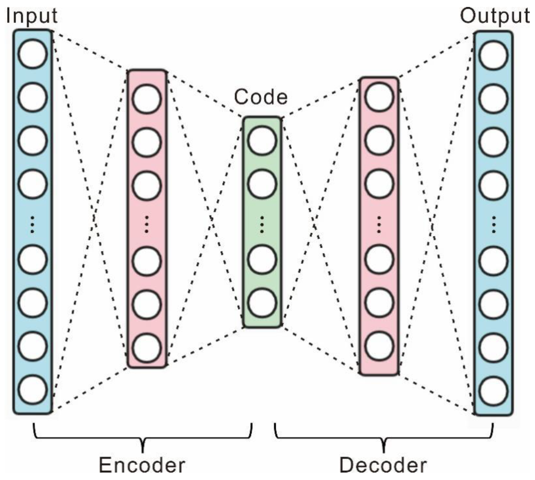
Figure 2.
The framework for Stacking ensemble learning.
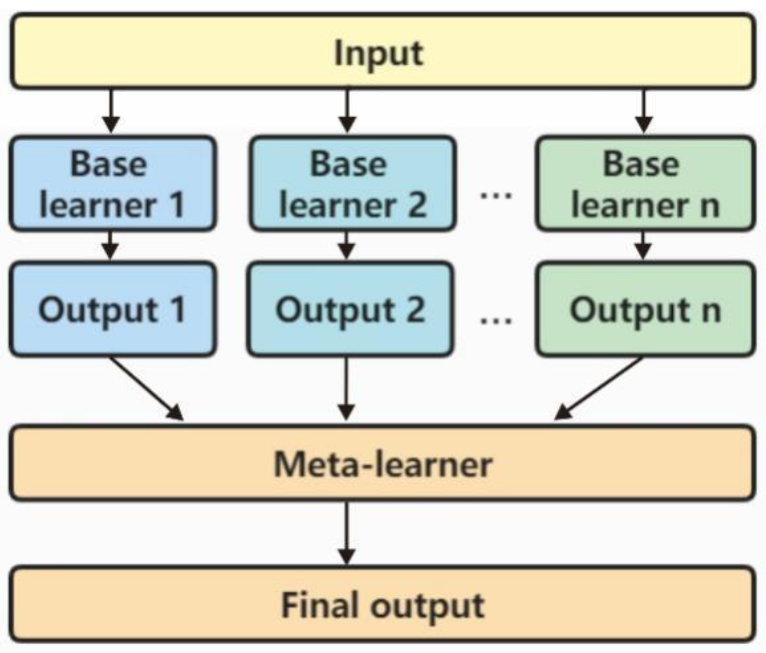
Figure 3.
Schematic diagram of k-fold cross validation.
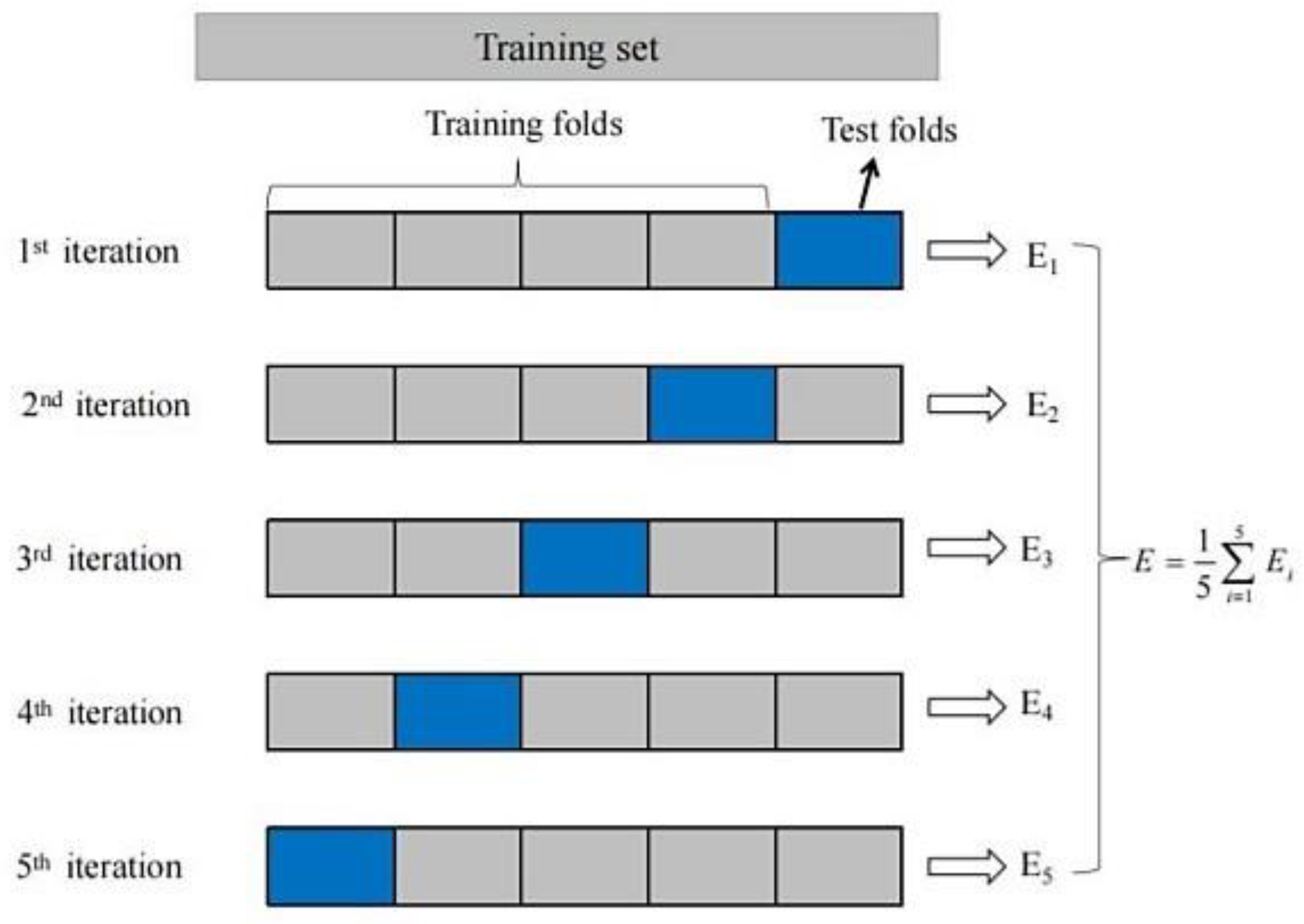
Figure 4.
Framework of SAE and StackingEL.
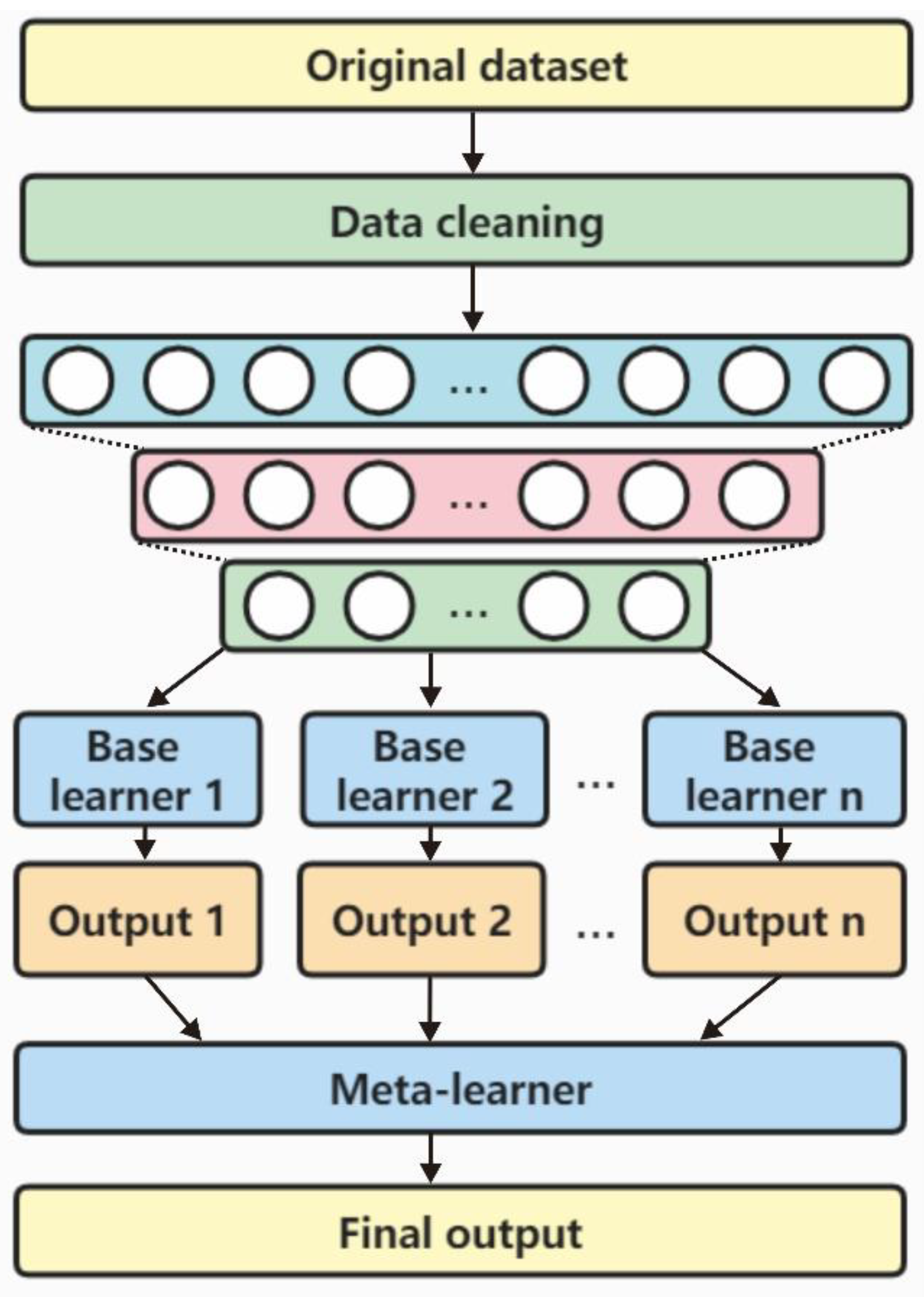
Figure 5.
Dimension selection of SAE.
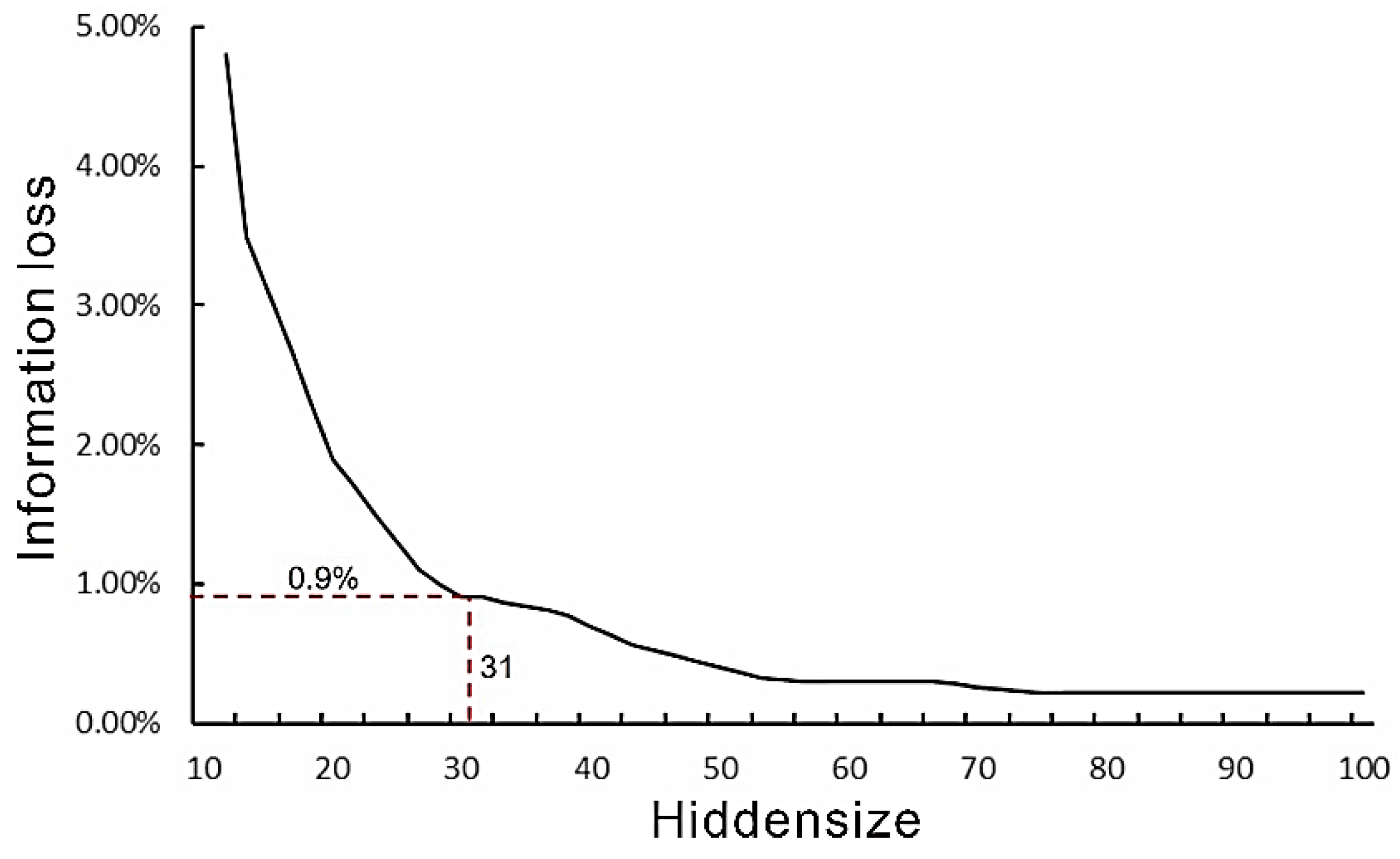
Figure 6.
The prediction results of the different model.
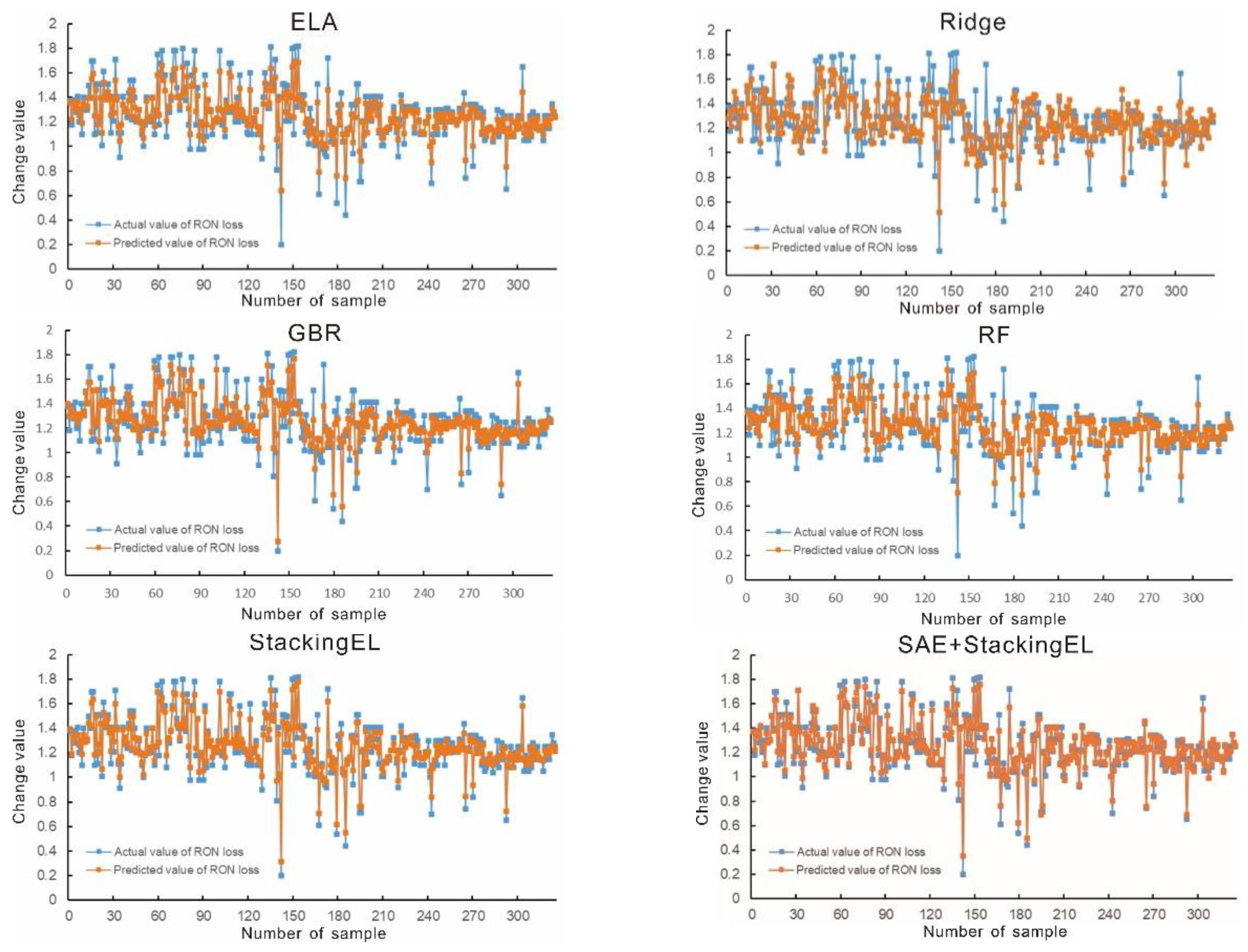

Table 1.
Accuracy of single prediction model.
| Evs | Meanae | Mse | Medianae | R2 | |
| Lasso | 0.5865 | 0.1002 | 0.0365 | 0.0905 | 0.5822 |
| Ridge | 0.7073 | 0.0088 | 0.0015 | 0.0090 | 0.7010 |
| SVR | 0.7056 | 0.0939 | 0.0152 | 0.0741 | 0.6985 |
| ElA | 0.8815 | 0.0561 | 0.0061 | 0.0420 | 0.8796 |
| NB | 0.2186 | 0.1463 | 0.0402 | 0.1087 | 0.2092 |
| LR | 0.2839 | 0.1402 | 0.0365 | 0.1017 | 0.2826 |
| RF | 0.8787 | 0.0571 | 0.0066 | 0.0379 | 0.8694 |
| GBR | 0.8556 | 0.0666 | 0.0076 | 0.0523 | 0.8505 |
| ERT | 0.3213 | 0.1362 | 0.0349 | 0.1017 | 0.3134 |
| XGB | 0.6039 | 0.0106 | 0.0023 | 0.0004 | 0.6000 |
| StackingEL | 0.9478 | 0.0457 | 0.0031 | 0.0412 | 0.9387 |
| SAE+StackingEL | 0.9657 | 0.0356 | 0.0021 | 0.0280 | 0.9578 |
Disclaimer/Publisher’s Note: The statements, opinions and data contained in all publications are solely those of the individual author(s) and contributor(s) and not of MDPI and/or the editor(s). MDPI and/or the editor(s) disclaim responsibility for any injury to people or property resulting from any ideas, methods, instructions or products referred to in the content. |
© 2025 by the authors. Licensee MDPI, Basel, Switzerland. This article is an open access article distributed under the terms and conditions of the Creative Commons Attribution (CC BY) license (http://creativecommons.org/licenses/by/4.0/).
Copyright: This open access article is published under a Creative Commons CC BY 4.0 license, which permit the free download, distribution, and reuse, provided that the author and preprint are cited in any reuse.


