Submitted:
30 August 2024
Posted:
30 August 2024
Read the latest preprint version here
Abstract
In this study, we consider the valuation of rainbow options using unsupervised machine learning methods. In particular, we consider the pricing of multi-asset (rainbow) European and American options, using Physics Informed Neural Net- works (PINNS). After developing the PINNS architecture, we benchmark the method by using it to price vanilla and exotic options with one and two un- derlying assets. We then use the methodology to price a multi-asset European option, followed by the pricing of the multi-asset American option by solving the linear complementarity problem. We compare our results to those obtained using preexisting numerical methods and note excellent agreement. Unlike con- ventional numerical methods, we note that this methodology does not suffer from the ’curse of dimensionality’. The time complexity of our method is con- siderably less than that of the conventional techniques. Thus PINNS may offer a faster more efficient solution to the pricing of rainbow options.
Keywords:
Qiuantitive finance
; option pricing
; rainbow options
; PINNs
; neural networks
1. Introduction
A significant portion of the financial instruments traded today are derivatives, whose values are derived from the performance of underlying assets such as stocks, bonds, indices, commodities, and interest rates. Options are among the most actively traded financial derivatives. An option is a contract that grants its holder the right, but not the obligation, to buy or sell underlying assets (such as stocks) at a predetermined price (strike price), on or before a specified date (expiry). There are two main options: call options (which provide the right to buy) and put options (which provide the right to sell). Investors use options for leverage and to hedge against financial risks. However, pricing these instruments can be mathematically challenging.
Options trading has a long history, with standardized options first traded on the Chicago Board Options Exchange (CBOE) on April 26, 1973. The Black-Scholes model Black andScholes (1973), developed by Fischer Black and Myron Scholes in 1973, provided a groundbreaking closed-form solution for pricing European options. This work earned Black and Scholes the Nobel Prize in Economics in 1997 and laid the foundation for more complex option pricing models and associated numerical methods. Over the decades, advanced models incorporating realistic assumptions have been developed, though explicit solutions are often not feasible. Consequently, various numerical methods have emerged, including binomial and trinomial trees, Monte Carlo simulations and finite difference and finite element schemes for solving partial differential equations (PDEs).
Boyle (1977) applied Monte Carlo simulation to the field of financial derivatives, this works by simulating a large number of random paths of the underlying asset’s price to estimate the value of any financial derivative. Broadie and Glasserman (1996) refined the Monte Carlo method for option pricing, particularly focusing on variance reduction techniques to improve computational efficiency. Longstaff and Schwartz (2001) gave a least-squares approach for valuing American Options by Monte-Carlo Simulations.
Cox et al. (1979) introduced the binomial tree method; a discrete-time model for option pricing that approximates the continuous-time process of the Black-Scholes model. Boyle et al. (1989) developed the trinomial tree model which offered better accuracy than the binomial model by incorporating an additional possible state at each node. Moon et al. (2008) extended the binomial model, typically applied to single-asset options, to multi-dimensional options.
Finite difference methods rely on discretizing a function on a grid. Courtadon (1983) extended the application of finite difference methods for solving the Black-Scholes partial differential equation, providing improved accuracy and stability. Liao and Khaliq (2009) proposed a fourth-order compact finite difference scheme to tackle a one-dimensional (1-D) nonlinear Black-Scholes equation, demonstrating unconditional stability. The application of the finite element method in option pricing by Andalaft-Chacur et al. (2011) offered a robust method for solving option pricing PDEs, particularly useful for American options and exotic derivatives with complex boundaries.
Finite elements were used to price multi-asset American options by Kaya (2011). The work of Seydel (2012) provides a thorough explanation and comparison of numerical methods for pricing financial derivatives, including finite difference methods. Wang et al. (2014) presented superconvergent fitted finite volume method for solving a degenerate nonlinear penalized Black-Scholes equation pertinent to European and American option pricing which was an improvement on conventional finite volume methods. Dilloo and Tangman (2017) suggested an advanced high-order finite difference method applicable to various option pricing models, encompassing the 1-D nonlinear Black-Scholes equation, Merton’s jump-diffusion model, and 2-D Heston’s stochastic volatility model. Koffi and Tambue (2022) introduced a distinctive finite volume method tailored for solving the Black-Scholes model involving two underlying assets. Mollapourasl et al. (2019) proposed a radial basis function combined with the partition of unity method for solving American options with stochastic volatility. Soleymani and Zhu (2021) devised a radial basis function-generated finite difference (RBF-FD) method to solve a stochastic volatility jump model represented as a 2-D PIDE.
The formalization of Artificial Neural Networks originated by McCulloch and Pitts (1943) as a programming paradigm inspired by biology, enabling computers to learn from observable data. The introduction of the error backpropagation learning algorithm by Rumelhart et al. (1986) greatly enhanced the appeal of neural networks (NNs) across diverse research fields. Today, NNs and deep learning are recognized as the most potent tools for addressing numerous challenges in image recognition, speech recognition, and natural language processing. They have also been applied to forecast and categorize economic and financial variables.
In the context of pricing financial derivatives, numerous studies have highlighted the benefits of employing neural networks (NNs) as a primary or supplementary tool. For example, Hutchinson et al. (1994) advocated the utilization of learning networks to estimate the value of European options. They asserted that learning networks could reconstruct the Black–Scholes formula by utilizing a two-year training set comprising daily options prices. The resulting network, according to their findings, could then be applied to derive prices and effectively delta-hedge options in out-of-sample scenarios. In their 2000 study, Garcia and Gençay (2000) derived a generalized option pricing formula with a structure akin to the Black–Scholes formula using a feed-forward neural network (NN) model. Their findings revealed minimal delta-hedging errors compared to the hedging effectiveness of the Black–Scholes model. Culkin (2017)’s study highlighted the transformative potential of deep learning in finance, demonstrating how advancements in technology and the accessibility of vast datasets have democratized the application of sophisticated neural network models for option pricing, marking a significant leap forward in the integration of artificial intelligence within the financial sector.
In the study by Han et al. (2018), the researchers redefined the high-dimensional nonlinear Black–Scholes (BS) equation as a set of backward stochastic differential equations (BSDEs) and approximated the solution’s gradient using deep neural networks. They illustrated the effectiveness of their deep BSDE method through a demonstration of a 100-dimensional problem. In a recent work by Eskiizmirliler et al. (2021), the researchers suggested resolving the one-dimensional Black–Scholes (BS) equation to predict the value of European call options. They achieved this by employing a feed-forward neural network, specifically one with a single hidden layer. Additional sources discussing the utilization of neural networks in option pricing and hedging can be explored in a recent review article by Ruf and Wang (2020).
Physics-Informed Neural Networks (PINNs) have shown promising results in solving partial differential equations (PDEs) by incorporating domain knowledge into the training process. Option pricing often involves solving complex PDEs, such as the Black-Scholes equation or more advanced models. Recently Gatta et al. (2023) used PINNs to price path-dependent options like American options. Also, PINNs have successfully been used to price two-dimensional European and American options by Wang et al. (2023) In this work we focus on the pricing of multi-asset ’Rainbow’ options (both American and European); such contracts enable investors to speculate on the relative performance of multiple underlying assets. Rainbow options have gained prominence due to their ability to capture correlations and interactions among various assets, making them a valuable tool for risk management. Rainbow options also play an important role in diversification and complex trading strategies.
The factors that determine the ease or difficulty of pricing and hedging multi-asset options include: (1) the existence of a closed-form solution (they usually lack closed-form solution), (2) the number of underlying assets i.e. the dimensionality, (3) path dependency, (4) early exercise.
In the absence of closed-form solutions, numerical methods have to be used for multi-asset option pricing. Choosing a suitable numerical scheme involves a combination of speed, accuracy, simplicity, and generality.
The challenge is mainly that with many of the schemes, the computational efforts grow exponentially with the problem’s dimensions. Some rainbow option problems have closed-form solutions; like exchange options or options with no path dependency and are relatively easy to price. For three or less dimensions, finite difference methods (FDM) or finite element methods (FEM) are efficient. They cope well with early exercise and many path-dependent features can be incorporated, though usually at the cost of an extra dimension. A more recent method for pricing rainbow options is the collection method. These methods work particularly well for low-dimensional problems. However, for higher dimensions, they become unstable and cannot provide accurate results.Wilmott (2006). For higher dimensions, Monte Carlo simulations are good. Unfortunately, they are not very efficient for American-style early exercise.
There is currently no numerical method that works very well with such a problem. As a result, the problem of efficiently pricing American rainbow option pricing for higher dimensions remains an interesting problem. This makes it a very interesting task to try and tackle with heuristic methods such as Physics Informed Neural Networks.
This paper is organized as follows. After the introduction and literature review in section 2, PINNs methodology is presented and the mathematical formulation of PINNs for option pricing PDEs is discussed in section 3. In section 4, we demonstrate the effectiveness and robustness of the proposed method for pricing options by comparing its results with existing methods. We benchmark the method by pricing a one-dimensional European option, a one-dimensional Asian option and two-dimensional cash or nothing option. In section 5, we use PINNs to calculate option prices for European and American style rainbow options with four underlying assets and disucss the efficiency and accuracy of the method. In section 6, we summarize our findings and discuss future work.
2. Methodology: Solving Option Pricing PDEs Using PINNs:
For a given differential equation:
in unknown function y along with appropriate boundary and/or initial conditions, PINNs approximates the solution , by using an ANN: , which is completely described by a set of parameters (weights) W. The given differential equation is taken to be the loss function of the neural network and the weights W are adjusted such that minimizes the loss function which is the same as saying that solves (to some accuracy) the given PDE. Here x represents the independent variables in the form of an n-tuple. After figuring out the domain of the independent variables, the points are randomly selected from that domain to act as inputs for our NN.
Vanilla or European Rainbow Option is a financial contract that gives the holder the right to buy/sell (call/put) assets ( for prescribed strike (S) at maturity . Since it allows the holder to exercise at a fixed maturity date, its payoff depends upon the price of the underlying stock at expiry only and not the path of underlying. Therefore it is a path-independent option. For the European option with number of underlying the associated PDE is:
where is the value of the option, each is the volatility of underlying stock , is the correlation coefficient between stock i&j , r is the interest rate, and is the time to expiry (T is the expiry, is instantaneous time). Equation (1) combined with payoff determines the price of the option
American Rainbow option is a financial contract that gives the holder the right to buy/sell (call/put) assets ( for prescribed strike (S) at any time up to and including maturity . This early exercise feature makes the American option valuation problem a free boundary problem i.e. there exists an unknown boundary, that depends upon time. This boundary acts as the decision surface between early exercise and holding the option and it has to be determined as a part of the problem. So for American option valuation, we rewrite the Black Scholes PDE (used to solve European options) to a linear complementary form: which implicitly includes the free boundary condition into the PDE.
Multi-asset American option in the Linear Complementary Problem (LCP) approach forms a multi-dimensional partial differential complementary problem (PDCP), as explained in chapter 7 of Wilmott et al. (1993);
However for this problem an analytical solution is not readily available. Since we want to convert black Scholes PDE into a Physics Informed Neural Network problem, first, we scale the input (stock) and adjust our PDE accordingly. Scaling is done to improve convergence, speed and stability during training. It prevents features with large magnitudes from dominating the optimization process, ensuring fair contributions from all features; as pointed out by Sola and Sevilla (1997). For scaling we substitute:
and These substitutions give us scaled PDE for the European Option:
and for American Option:
To convert the above black Scholes pde for European option with multiple underlying into a Physics Informed Neural Network problem, first, we describe our pde in general form as
in the interior of domain
or any other Boundary condition, on the boundary of the domain
Similarly to convert the American Option pricing problem to a Physics Involve Neural Network problem, let’s describe our PDE in general form as
in the interior of domain
or any other Boundary condition, on the boundary of the domain.
Here and are the differential operators on the domain and boundary respectively. In PINNs, the initial conditions are treated the same as the boundary conditions. We select (randomly) a collection of interior and boundary points , where each point is in an n-tuple of size (for d=number of stocks and extra one dimension to accommodate time ) The solution of any differential equation using PINNs involves minimizing a single loss function which includes all constraints:
Minimizing means we are trying to find i.e. a set of weights W for which the PDE, is zero or as close to zero as possible and the boundary conditions are also met, i.e. solves the PDE.
To check the efficiency of our models we calculate the mean square root of error (RMSE) and relative error of our model against any preexisting solution method .
3. Benchmarking
We now use the PINNs methodology to solve some well-understood problems. We will compare our results with those in the literature. We have trained our Neural Networks using T4GPU on Google Colab.
3.1. Bench Marking with One-Dimensional Linear Case:
First, we will consider solving the standard Black Scholes PDE equation for one underlying stock, obtained by putting in equation(3):
The price of the European put Option is obtained by solving the above BSPDE subject to these conditions:
where L is some suitably large value obtained by truncating the original domain to . We take . This is a rather simple problem that has an explicit solution. The exact solution of this BSPDE can be found in Ch7 Wilmott (2006)
We solve this model for the following parameters:
These parameters are the same as the ones used in Wang et al. (2023).
We have two inputs (scaled stock price and time to expiry) and one output (scaled option price). We use a fully connected neural network with depth 4 (ie 3 hidden layers) and width 20 i.e. 20 neurons in each layer. For a fully connected feed forward neural network, the weights between two layers are equal to the number of neurons in the first layer multiplied by the number of neurons in the second layer, plus one bias weight per neuron in the second layer, which means our model has 921 weights. We use 2000*4 training residual points sampled inside the spatio-temporal domain, 200*4 training points sampled on the boundary, and 100*4 residual points for the initial conditions. The activation function is the hyperbolic tangent (tanh). We first use Adam for 1000 iterations with a learning rate of 0.001, and then switch to L-BFGS. The L-BFGS does not require a learning rate, and the neural network is trained until convergence. The number of training points, iterations, and the structure of the NN are decided upon careful consideration and trying different values until one with the best convergence and least L2 score is figured out.
The train loss for ’Adam’ is 1.26e-03, and ’train’ took 4.4 seconds; while the train loss for ’L-BFGS’ is 2.50e-06 and ’train’ took 40.64 seconds.
Figure 1 shows the test train loss history
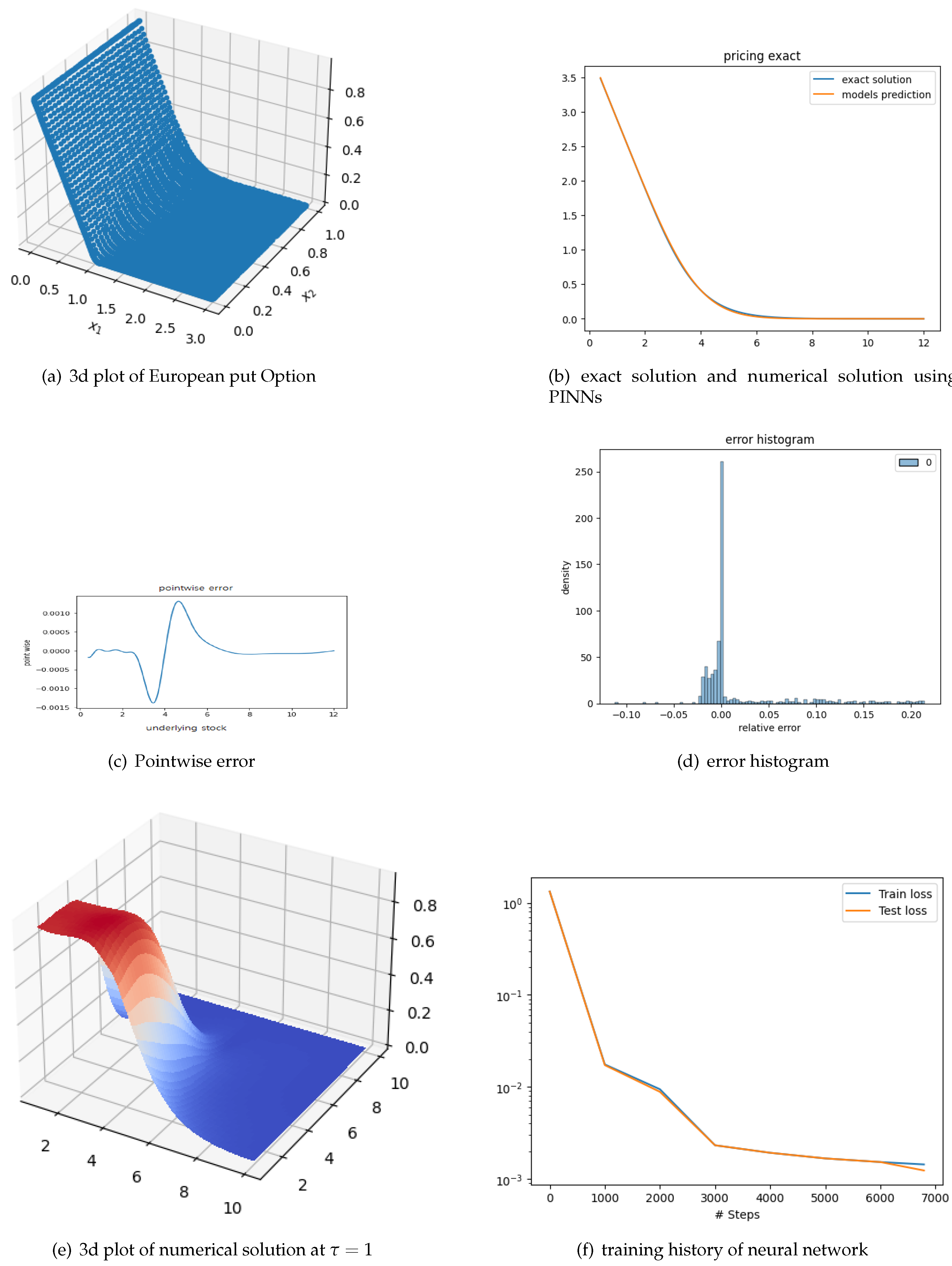
Figure 2a shows the 3d plot of numerical solution over whole time domain where and . For error comparison, first, we convert the output of our PINNs which is the scaled price (), to option price () by using the relation:
In Figure 2b, we plot the numerical solution using PINNs against the exact solution calculated using formulas from Wilmott et al. (1993) at . In Figure 2c, we plot the corresponding pointwise error (calculated as the predicted solution - exact solution), over the whole stock space . In Figure 2d, we show the error histogram by taking 1000 random points from the domain . The relative error is 0.00548 which is very small and quite acceptable.
3.2. Benching Marking with Two-Dimensional Put Option
In this section, we consider the two-asset option pricing problem, which is governed by the following PDE obtained by substituting in equation(3)
where option value depends upon prices of underlying asset and time to maturity . The payoff function for cash or nothing put option is:
where is a fixed amount. For comparison we choose the same model parameters as by Wang et al. (2023)
The physical domain is truncated to a bound rectangle: and
Dirichlet boundary conditions are imposed on and . On , the boundary condition is chosen as the one-dimensional European binary put option on , which is
where
and is the cumulative distribution function. By the same argument, the boundary condition on is given by
where
Here We have three inputs (price of stock one, price of stock two and time to expiry) and one output (cash or nothing put option price). We use a fully connected neural network with depth 6 (which means 5 hidden layers) and width 30. There are 3871 weights in this NN.
We use 2000*10 training residual points sampled inside the spatio-temporal domain, 200*10 training points sampled on the boundary, and 100*10 residual points for the initial conditions. The activation function is the hyperbolic tangent (tanh). We first use Adam for 2000 iterations with a learning rate of 0.001, and then switch to L-BFGS. The L-BFGS does not require a learning rate, and the neural network is trained until convergence. The train loss for ’Adam’ is 1.47e-02, and ’train’ took 22.975904 seconds; while the train loss for ’L-BFGS’ is 1.56e-03, and ’train’ took 73.832366 seconds.
Figure 2f shows the test train loss history
The obtained numerical solution plot is shown in Figure 2e. It shows the 3d plot of the numerical solution at final time T or time to expiry zero, the x-axis and y-axis in the plot represent the two underlying stocks. The plot is visually similar to Figure 5 in , Wang et al. (2023)
3.3. Bench Marking with One-Dimensional Path-Dependent Option
Pricing Asian average rate call Options we introduce a new variable
and solve the system of PDEs
and
subject to the terminal condition of option price:
and initial condition of average
boundary conditions for this average rate call options are:
where L is some suitably large value by truncating the original domain to . We take .
A singularity exists in the equation for A at (i.e., today). However, at the term also goes to zero leaving us with a BSPDE for the European option which has an exact solution. so we leave out t=0 and take our time domain as or ((Hozman and Tichý (2017))
We solve this model problem with parameters:
Note that for an Asian option, we use the actual time instead of introducing because t appears explicitly in this pde. We have two inputs (scaled stock price and time to expiry) and two outputs (average price, and option price). We use a fully connected neural network with depth 4 (ie 3 hidden layers) and width 20. Thus there are 942 weights. We use 2000*10 training residual points sampled inside the spatio-temporal domain, 200*10 training points sampled on the boundary, and 100*10 residual points for the initial conditions. The activation function is the hyperbolic tangent (tanh). We first use Adam for 5000 iterations with a learning rate 0.001 and then switch to L-BFGS which works until convergence
The train loss for ’Adam’ is 2.94e-01, and ’train’ took 13.9 seconds; while the train loss for ’L-BFGS’ is 2.76e-01 and ’train’ took 4.64 seconds.
For error comparison we randomly generated 1000 data points from the input domain of our NN i.e. . The first coordinate of the out point represents the initial value of stock and the other represents a time to expiry(t). Then we calculated the option value for those points using the Monte Carlo method with 100000 paths and 256 time steps. We also calculate the values our model predicts for each point. The relative error is calculated using the formula:
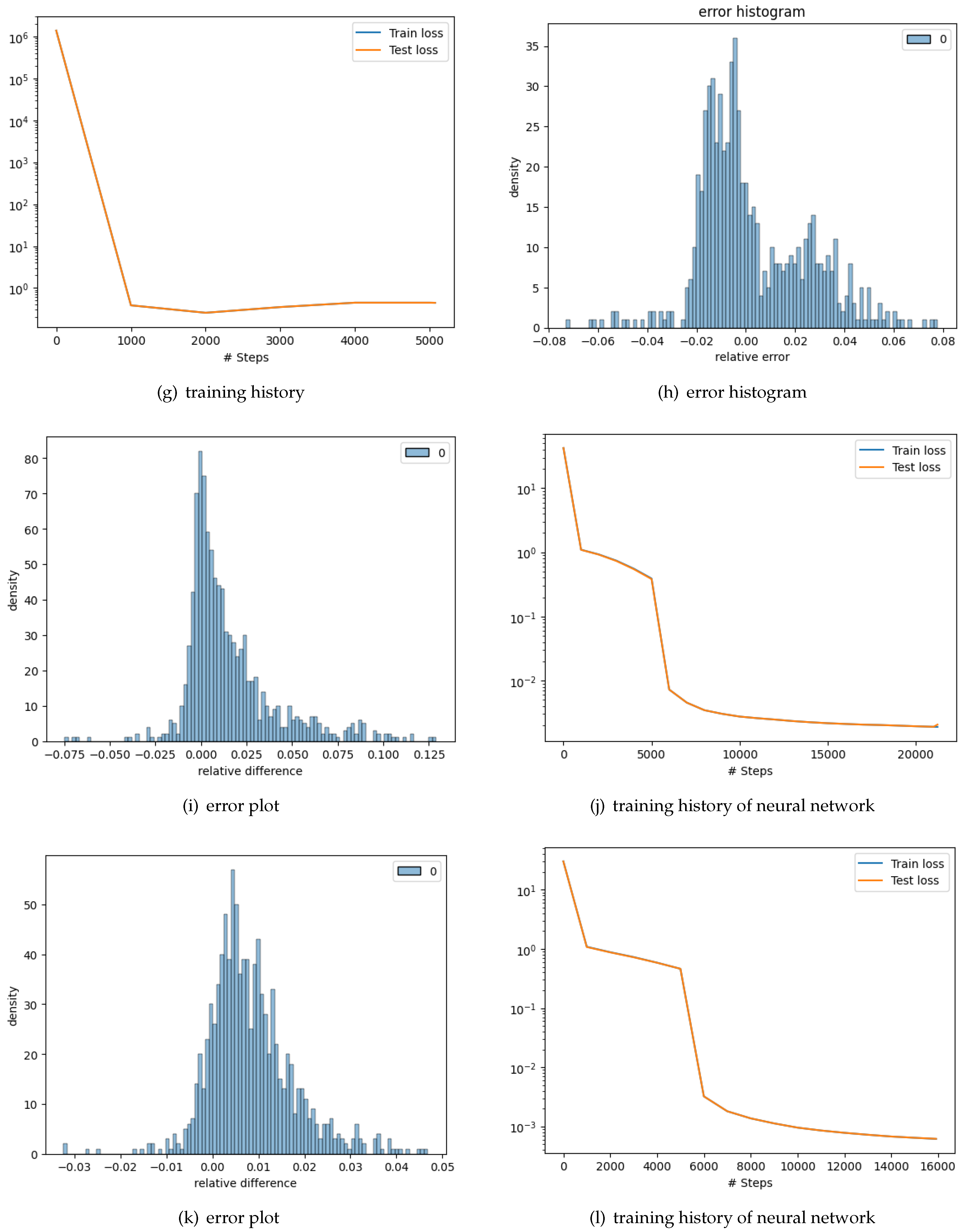
We plot an error histogram, to evaluate our results Culkin (2017). The root-mean-squared error (RMSE) is 0.0041, which may be compared to the fact that the strike prices are all normalized to $1. Hence the average error is less than ±4% of the strike. The average percentage pricing error (error divided by option price) is 0.0220 i.e., almost 2%. The histogram of pricing errors is shown 3(i). We see that the errors are sufficiently small. Further, we estimated a regression of the model values and obtained R2 = 0.9981, i.e. almost 99.9% which is quite acceptable.
4. Pricing of Rainbow Options
We now turn to the problem of pricing rainbow options. We will consider both American and European options in our study. We will compare our results to those obtained using existing methods and show that the method is comparable in accuracy to the existing techniques while being faster at the same time.
4.1. Pricing of European Call Options with Four Underlying Stocks
The scaled PDE for the European call option that will act as the loss function of our PINNs will be:
which is obtained by substituting in equation(3). The initial condition for the max call option is:
Unlike for the one-dimensional or two-dimensional cases, we don’t have clear values at the stock boundary but for the multi-dimension call option we can impose this Boundary condition at boundary
for any
We took all our underlying stocks, to be in the domain ; where L is sufficiently large.( ). Since our input, is scaled as our is in the domain for each stock. We take these parameters for our option
- Strike Price 100 ,
- Maturity 1 year,
- Risk-free rate 0.01,
- volatility of stocks 0.08 ,
- correlation between stocks 0.5
To train the network we sampled uniformly 2000*10 training residual points, inside the spatio-temporal domain, 200*10 training points on the boundary, and 100*10 residual points for the initial conditions. We have five inputs (price of stock one, price of stock two, price of stock three, price of stock four and time to expiry) and one output (multi-asset max call option price). We choose a fully connected neural network of depth 3 (i.e. 2 hidden layers) and width 20. So there are 561 weights. We start with "tanh" as the activation switch. After defining the neural network we build the model; choosing "adam" as the optimizer and "" learning rate for "5000" iterations where an iteration is the number of times a certain batch is passed via an algorithm. After training with "adam" we train with "L-BFGS" until convergence.
The train loss for Adam is 3.89e 01, and ’train’ took 60.770858 seconds; while the train loss for ’L-BFGS’ is 1.89e-03 ’train’ took 248.284244 s seconds. Figure 2j shows the test train loss history
For error comparison we generate option values for 1000 data points using another numerical solution, the Monte Carlo method with 100000 paths and 256 time steps. To evaluate our solution we plot the error histogram. The root-mean-squared error (RMSE) is 0.00965, which may be compared to the fact that the strike prices are all normalized to $1. Hence the average error is less than ±1% of the strike. The average percentage pricing error (error divided by option price) is 0.0312, i.e., almost 3.1%. The histogram of pricing errors is shown 3(i). We see that the errors are very small. Further, we estimated a regression of the model values and obtained an R2 = 0.9856, which is almost 99% i.e. very high.
4.1.1. American Option PINNs for Four Underlying
The scaled PDE for the American call option that will act as the loss function of our PINNs will be:
where g is the initial condition
The same problem parameters as in the European option’s case are also used for the American option. We also take the same model parameters and training points as for the European 4D call option. The train loss for ’Adam’ is 4.62e-01, and ’train’ took 60.803890 seconds; while the train loss for ’L-BFGS’ is 6.12e-04’ train’ took 159.804906 s seconds. Figure 2l shows the test train loss history
Just like we did in the case of the European multi-asset option, for error comparison we generate option values for 1000 data points using Monte Carlo with 100000 paths and 256 time steps. To evaluate our result we plot error histogram. The root mean-squared error (RMSE) is 0.0014, which may be compared to the fact that the strike prices are all normalized to $1. Hence the average error is less than ±0.15% of the strike. The average percentage pricing error (error divided by option price) is 0.0138, i.e. 1.4% of option price. The histogram of pricing errors is shown in Figure 2k. which shows that the errors are very small. Further, we estimated a regression of the model values and obtained an R2 = 0.9977 , which is very high. Thus the model gives very good results.
For time comparison we saw that determining the European option’s (with four underlying stocks) values using the Monte Carlo method with 100000 paths and 256 time steps required 661.8950 seconds. Conversely, training and generating the value of an option using PINNs took 312.8564 seconds, meaning a 52.73% improvement. Determining the American option’s (with four underlying stocks) values using the Monte Carlo method with 100000 paths and 256 time steps required 1128.2052 seconds. Conversely, training and generating the value of an option using PINNs took 223.7130 seconds which means an 80.17 improvement. Also employing a trained neural network to calculate the option value always took less than 0.2 seconds which is very fast and can be of great use in case one is racing against time. This substantial enhancement in time efficiency underscores the efficacy of neural networks, Also a very interesting observation is that NN converges faster and better for the American Option than it does for the European option, which points towards the phenomenon that the complexity of the PDE does not affect the speed and performance of PINNs negatively.
5. Conclusion
In this study we considered the pricing of rainbow options (options with multiple underlying) using PINNs. After benchmarking the method we set up the training time of Physics-Informed Neural Networks (PINNs) is influenced by various factors such as the partial differential equation (PDE), boundary conditions (BCs), and the neural network architecture. However, our findings demonstrate that the training time does not exhibit exponential growth with the increase in the number of inputs. Notably, our experimentation reveals that the 4D Euro option required less training time compared to the 2D option.
When it comes to pricing multi-asset options, particularly American options which pose significant computational challenges, PINNs exhibit promising outcomes. Leveraging AI and neural networks, which are rapidly evolving fields, in option pricing not only showcases current effectiveness but also opens avenues for leveraging future advancements in AI and PINNs. Once the network is trained, the option pricing process becomes almost instantaneous, significantly faster than existing algorithms. Moreover, we observed substantial improvements in time efficiency, especially when generating values across multiple stocks and time intervals for the same option.
References
- Andalaft-Chacur, A., Ali, M. M., and Salazar, J. G. (2011). Real options pricing by the finite element method,. Computers and Mathematics with Applications, 16:2863–2873. [CrossRef]
- Black, F. and Scholes, M. (1973). The pricing of options and corporate liabilities. Journal of Political Economy, 81(3):637–654. [CrossRef]
- Boyle, P. P. (1977). Options: A monte carlo approach. Journal of Financial Economics, 4(3):323–338. [CrossRef]
- Boyle, P. P., Evnine, J., and Gibbs, S. (1989). Numerical evaluation of multivariate contingent claims. Review of Financial Studies, 2(2):241–250. [CrossRef]
- Broadie, M. and Glasserman, P. (1996). Estimating security price derivatives using simulation. Management Science, 42(2):269–285. [CrossRef]
- Courtadon, G. (1983). A more accurate finite difference approximation for the valuation of options. Journal of Financial and Quantitative Analysis, 17(5):697–703. [CrossRef]
- Cox, J. C., Ross, S. A., and Rubinstein, M. (1979). Option pricing: A simplified approach. Journal of Financial Economics, 7(3):229–263. [CrossRef]
- Culkin, R. (2017). Machine learning in finance: The case of deep learning for option pricing. computer science.
- Dilloo, M. J. and Tangman, D. Y. (2017). A high-order finite difference method for option valuation. Computers & Mathematics with Applications, 74(4):652–670.
- Eskiizmirliler, S., Günel, K., and Polat, R. (2021). On the solution of the black-scholes equation using feed-forward neural networks. Computational Economics, 58:915–941. [CrossRef]
- Garcia, R. and Gençay, R. (2000). Pricing and hedging derivative securities with neural networks and a homogeneity hint. Journal of Econometrics, 94(1-2):93–115.
- Gatta, F., Di Cola, V. S., Giampaolo, F., Piccialli, F., and Cuomo, S. (2023). Meshless methods for american option pricing through physics-informed neural networks. Engineering Analysis with Boundary Elements, 151:68–82. [CrossRef]
- Han, J., Jentzen, A., and Ee, W. (2018). Solving high-dimensional partial differential equations using deep learning. Proceedings of the National Academy of Sciences, 115(34):8505–8510. [CrossRef]
- Hozman, J. and Tichý, T. (2017). Dg method for numerical pricing of multi-asset asian options—the case of options with floating strike. Applied Mathematics, 62:171–195. [CrossRef]
- Hutchinson, J. M., Lo, A. W., and Poggio, T. (1994). A nonparametric approach to pricing and hedging derivative securities via learning networks. The journal of Finance, 49(3):851–889.
- Kaya, D. (2011). Pricing a Multi-Asset American Option in a Parallel Environment by a Finite Element Method Approach. PhD thesis, Uppsala University, Department of Mathematics.
- Koffi, R. S. and Tambue, A. (2022). A fitted l-multi-point flux approximation method for pricing options. Computational Economics, 60:633 – 663. [CrossRef]
- Liao, W. and Khaliq, A. Q. M. (2009). High-order compact scheme for solving nonlinear black–scholes equation with transaction cost. International Journal of Computer Mathematics, 86(6):1009–1023. [CrossRef]
- Longstaff, F. A. and Schwartz, E. S. (2001). Valuing american options by simulation: A simple least-squares approach. Review of Financial Studies, 14(1):113–147. [CrossRef]
- McCulloch, W. S. and Pitts, W. (1943). A logical calculus of the ideas immanent in nervous activity. Bulletin of Mathematical Biophysics, 5(10):115–113. . Reprinted in McCulloch 1964, pp. 16–39.
- Mollapourasl, R., Fereshtian, A., and Vanmaele, M. (2019). Radial basis functions with partition of unity method for american options with stochastic volatility. Computational Economics, 53:259–287. [CrossRef]
- Moon, K.-S., Kim, W.-J., and Kim, H. (2008). Adaptive lattice methods for multi-asset models. Computers & Mathematics with Applications, 56(2):352–366. [CrossRef]
- Ruf, J. and Wang, W. (2020). Neural networks for option pricing and hedging: a literature review. Journal of Computational Finance, 24(1):1–45. [CrossRef]
- Rumelhart, D., Hinton, G., and Williams, R. (1986). Learning representations by back-propagating errors. Nature, 323:533–536. [CrossRef]
- Seydel, R. U. (2012). Tools for Computational Finance. Springer, 5th edition.
- Sola, J. and Sevilla, J. (1997). Importance of input data normalization for the application of neural networks to complex industrial problems. IEEE Transactions on Nuclear Science, 44(3):1464–1468.
- Soleymani, F. and Zhu, S. (2021). Rbf-fd solution for a financial partial-integro differential equation utilizing the generalized multiquadric function. Computers & Mathematics with Applications, 82(15):161–178.
- Wang, S., Zhang, S., and Fang, Z. (2014). A superconvergent fitted finite volume method for black-scholes equations governing european and american option valuation: Superconvergent fitted finite volume method. Numerical Methods for Partial Differential Equations, 31(4):1190–1208.
- Wang, X., Li, J., and Li, J. (2023). A Deep Learning Based Numerical PDE Method for Option Pricing. Computational Economics, 62(1):149–164.
- Wilmott, P. (2006). Paul Wilmott on Quantitative Finance. John Wiley and Sons, second edition.
- Wilmott, P., Dewynne, J., and Howison, S. (1993). Option Pricing: Mathematical Models and Computation. Oxford Financial Press.
Figure 1.
training history
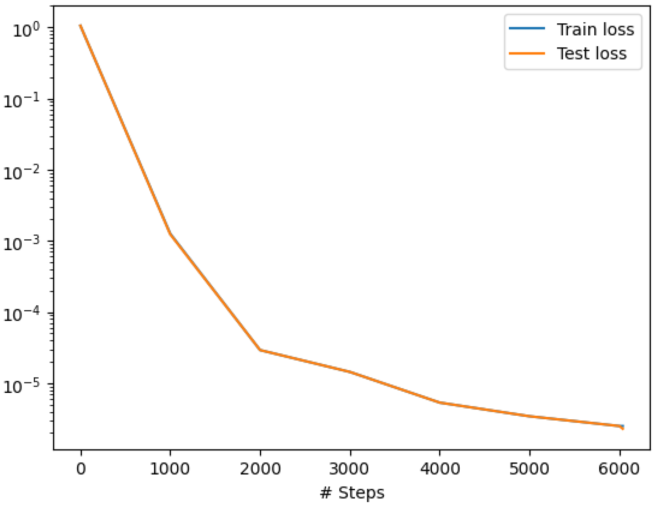
Figure 2.
Disclaimer/Publisher’s Note: The statements, opinions and data contained in all publications are solely those of the individual author(s) and contributor(s) and not of MDPI and/or the editor(s). MDPI and/or the editor(s) disclaim responsibility for any injury to people or property resulting from any ideas, methods, instructions or products referred to in the content. |
© 2024 by the authors. Licensee MDPI, Basel, Switzerland. This article is an open access article distributed under the terms and conditions of the Creative Commons Attribution (CC BY) license (http://creativecommons.org/licenses/by/4.0/).
Copyright: This open access article is published under a Creative Commons CC BY 4.0 license, which permit the free download, distribution, and reuse, provided that the author and preprint are cited in any reuse.


