
Submitted:
21 July 2025
Posted:
22 July 2025
You are already at the latest version
Abstract
This study presents a comparative analysis of supervised and unsupervised neural network approaches for pricing multi-asset options, with a particular focus on exchange options involving two underlying assets. The supervised methodology utilises data-driven neural networks trained on simulated option prices. In contrast, the unsupervised approach employs Physics-Informed Neural Networks that incorporate the governing partial differential equation along with boundary and initial conditions directly into the loss function. Addressing a notable gap in the literature, this work evaluates the relative efficiency of PINNs and supervised neural networks in pricing multi-asset derivatives. Additionally, we propose a novel grid search framework to systematically identify optimal hyperparameters for both approaches, enabling a fair comparison in terms of accuracy, computational speed, and overall efficiency. Empirical results indicate that the supervised neural network outperforms the PINNs approach, achieving superior accuracy and significantly reduced execution times, which underscores its suitability for real-time financial applications. However, the findings also highlight that PINNs remain a valuable alternative in scenarios where data availability is limited, offering a flexible model-free solution for complex option pricing problems.
Keywords:
multi-asset options
; artificial neural networks
; option pricing
; physics-informed neural networks (PINNs)
; exchange options
1. Introduction
A substantial share of today’s financial markets is comprised of derivatives—financial instruments whose value depends on the performance of underlying assets such as stocks, bonds, indices, commodities, or interest rates. Among these, options are among the most actively traded. An option is a contract granting the holder the right, but not the obligation, to buy or sell an underlying asset at a predetermined strike price, either on or before a specified expiry date. The two primary types of options are calls, which confer the right to buy, and puts, which confer the right to sell. Investors commonly use options to gain leverage or to hedge against financial risks. Despite their usefulness, accurately pricing options poses significant computational challenges
Options trading has a long history, with standardized options first traded on the Chicago Board Options Exchange (CBOE) on April 26, 1973. The Black-Scholes model ([17]), developed by Fischer Black and Myron Scholes in 1973, provided a groundbreaking closed-form solution for pricing European options. This work earned Black and Scholes the Nobel Prize in Economics in 1997 and laid the foundation for more complex option pricing models and associated numerical methods. Over the decades, advanced models incorporating realistic assumptions have been developed, though explicit solutions are often not feasible. Consequently, various numerical methods have emerged, including binomial and trinomial trees, Monte Carlo simulations and finite difference and finite element schemes for solving partial differential equations (PDEs).
[10] applied Monte Carlo simulation to the field of financial derivatives, this works by simulating a large number of random paths of the underlying asset’s price to estimate the value of any financial derivative. [11] refined the Monte Carlo method for option pricing, particularly focusing on variance reduction techniques to improve computational efficiency.
[13] introduced the binomial tree method; a discrete-time model for option pricing approximates the Black-Scholes model’s continuous-time process. [9] developed the trinomial tree model which offered better accuracy than the binomial model by incorporating an additional possible state at each node. [30] extended the binomial model, typically applied to single-asset options, to multi-dimensional options.
[12] extended the application of finite difference methods for solving the Black-Scholes partial differential equation, providing improved accuracy and stability. [25] proposed a fourth-order compact finite difference scheme to tackle a one-dimensional (1-D) nonlinear Black-Scholes equation, demonstrating unconditional stability. The application of the finite element method in option pricing by [27] offered a robust method for solving option pricing PDEs, particularly useful for exotic derivatives with complex boundaries.
[35] presented a superconvergent fitted finite volume method for solving a degenerate nonlinear penalized Black-Scholes equation, which was an improvement on conventional finite volume methods. [15] suggested an advanced high-order finite difference method applicable to various option pricing models, encompassing the 1-D nonlinear Black-Scholes equation, Merton’s jump-diffusion model, and 2-D Heston’s stochastic volatility model. [24] introduced a distinctive finite volume method tailored for solving the Black-Scholes model involving two underlying assets.
Although these methods are effective, they face practical limitations. For example, assumptions like constant volatility often fail to align with dynamic market conditions, leading to inaccuracies. Additionally, high-dimensional problems, such as those encountered with basket or exotic options, pose considerable computational challenges, often referred to as the "curse of dimensionality." While improvements in numerical methods have addressed some of these challenges, they often require substantial computational resources and increased complexity.
The formalization of Artificial Neural Networks originated by [28] as a programming paradigm inspired by biology, enabling computers to learn from observable data. The introduction of the error backpropagation learning algorithm by [7] greatly enhanced the appeal of neural networks (NNs) across diverse research fields. Today, NNs and deep learning are recognized as the most potent tools for addressing numerous challenges in image recognition, speech recognition, and natural language processing. They have also been applied to forecast and categorize economic and financial variables.
In the context of pricing financial derivatives, numerous studies have highlighted the benefits of employing neural networks (NNs) as a primary or supplementary tool. For example, [22] advocated the utilization of learning networks to estimate the value of European options. They asserted that learning networks could reconstruct the Black–Scholes formula by utilizing a two-year training set comprising daily options prices. The resulting network, according to their findings, could then be applied to derive prices and effectively delta-hedge options in out-of-sample scenarios. In their 2000 study, [18] derived a generalized option pricing formula with a structure akin to the Black–Scholes formula using a feed-forward neural network (NN) model. Their findings revealed minimal delta-hedging errors compared to the hedging effectiveness of the Black–Scholes model. [14]’s study highlighted the transformative potential of deep learning in finance, demonstrating how advancements in technology and the accessibility of vast datasets have democratized the application of sophisticated neural network models for option pricing, marking a significant leap forward in the integration of artificial intelligence within the financial sector.
In the study by [20], the researchers redefined the high-dimensional nonlinear Black–Scholes (BS) equation as a set of backward stochastic differential equations (BSDEs) and approximated the solution’s gradient using deep neural networks. They illustrated the effectiveness of their deep BSDE method through a demonstration of a 100-dimensional problem. In a recent work by [16], the researchers suggested resolving the one-dimensional Black–Scholes (BS) equation to predict the value of European call options. They achieved this by employing a feed-forward neural network, specifically one with a single hidden layer. Additional sources discussing the utilization of neural networks in option pricing and hedging can be explored in a recent review article by [31].
Physics-Informed Neural Networks (PINNs) have shown promising results in solving partial differential equations (PDEs) by incorporating domain knowledge into the training process. Option pricing often involves solving complex PDEs, such as the Black-Scholes equation or more advanced models. Recently [19] used PINNs to price path-dependent options like American options. Also, PINNs have successfully been used to price two-dimensional European and American options by [36]. [42] have successfully priced multiasset, path-dependent options using PINNs.
In this work we focus on the pricing of multi-asset options; such contracts enable investors to speculate on the relative performance of multiple underlying assets. Multi-asset options have gained prominence due to their ability to capture correlations and interactions among various assets, making them a valuable tool for risk management. They also play an important role in diversification and complex trading strategies.
In the absence of closed-form solutions, numerical methods have to be used for multi-asset option pricing. Choosing a suitable numerical scheme involves a combination of speed, accuracy, simplicity, and generality. There is currently no comparison done on the efficiency of PINNs and supervised learning for pricing multi-asset options. We aim to address this gap in our work.
This paper is organized as follows. After the introduction and literature review in section 2, two types of Neural network methodologies (supervised and unsupervised) are presented. The mathematical formulation of Supervised Neural networks and unsupervised neural networks (PINNs) for option pricing PDEs is discussed in section 3. In section 4, we benchmark neural network-based approaches on the standard Black-Scholes Partial Differential Equation (PDE) for a European call option on a single asset, using both supervised learning and Physics-Informed Neural Networks (PINNs). In section 5, we extend the methodology to two underlying assets and use supervised neural networks and PINNs to calculate option prices for exchange options and discuss the efficiency and accuracy of the two methods we also compare the two approaches. In section 6, we summarize our findings and discuss future work.
2. Methodology: Option Pricing Using Neural Networks:
The pricing of a European-style multi-asset option, denoted as , is governed by the following partial differential equation (PDE):
where represents the volatility of the underlying asset , denotes the correlation coefficient between assets and , r is the risk-free interest rate, and is the time to expiry. The solution to Equation (1), subject to the terminal condition , determines the option price .
To reformulate the Black–Scholes Partial Differential Equation (BSPDE) within any neural net framework (supervised or unsupervised), it is necessary to first apply a suitable transformation to the input variables. This preprocessing step, referred to as scaling, enhances convergence speed, stability, and numerical efficiency during training. By ensuring that all features contribute equitably to the optimization process, scaling mitigates the dominance of variables with large magnitudes, as highlighted in [33]. Specifically, we introduce the following transformations:
where S is a constant chosen based on the structure of the option’s payoff function, for example, the strike price. Applying these substitutions yields this scaled PDE for the European option:
2.1. Supervised Approach for Pricing Options
In the supervised learning approach for solving differential equations using neural networks, a set of randomly sampled points, , is selected from the domain to construct a dataset. In this dataset, each serves as the input where
while represents the corresponding output. In our case, output is the option value at the input point, computed using a conventional solver. Formally, the dataset is defined as:
A neural network is then trained to approximate the mapping:
where the network’s weights, W, are optimized by minimizing the loss function . Once trained, the neural network can be used to approximate solutions for any new input values.
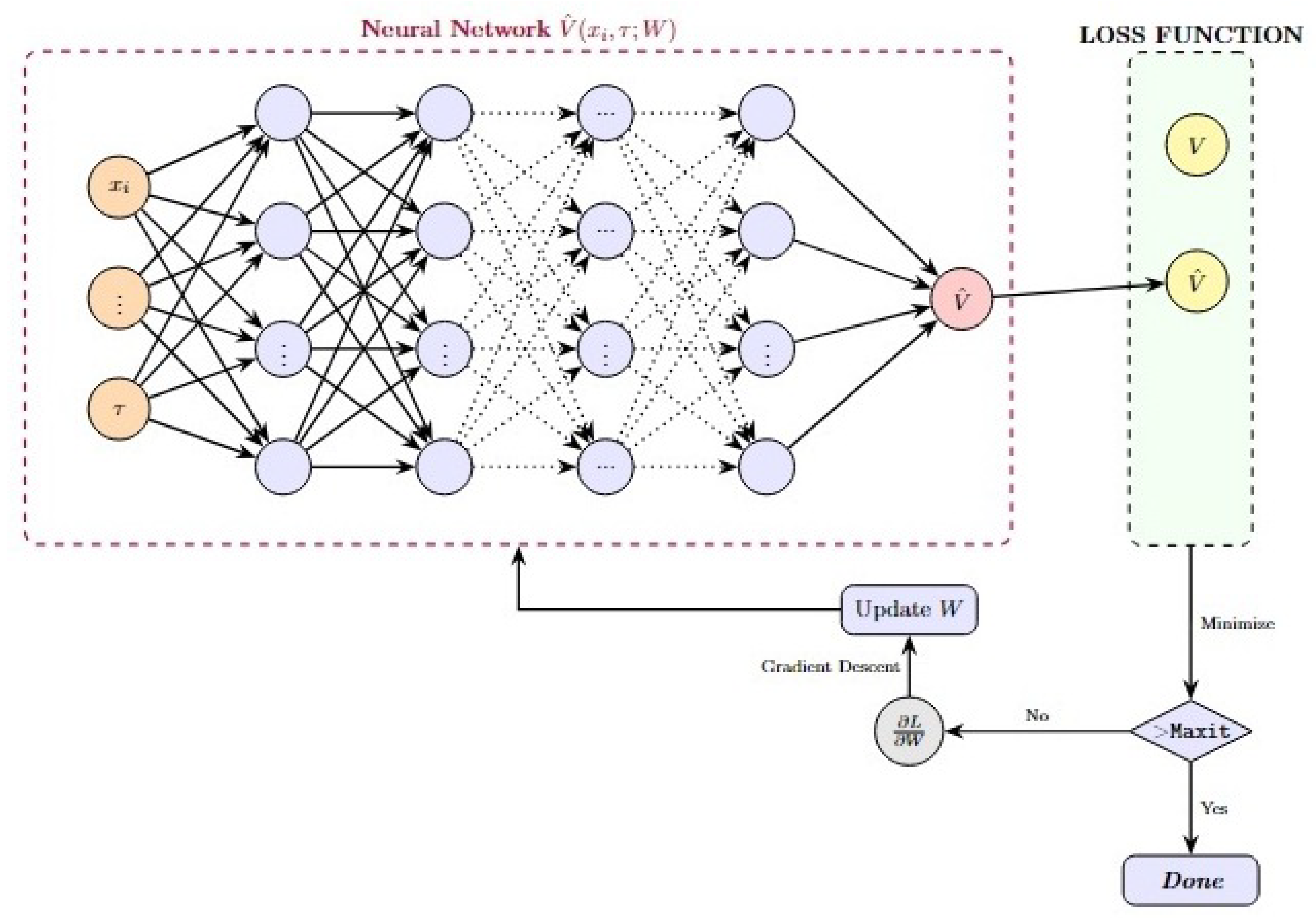
Figure 1.
Supervised Learning Training Scheme for Option Pricing.
| Algorithm 1 Supervised Neural Network Training for Option Pricing |
|
2.2. Unsupervised Approach for Pricing Options
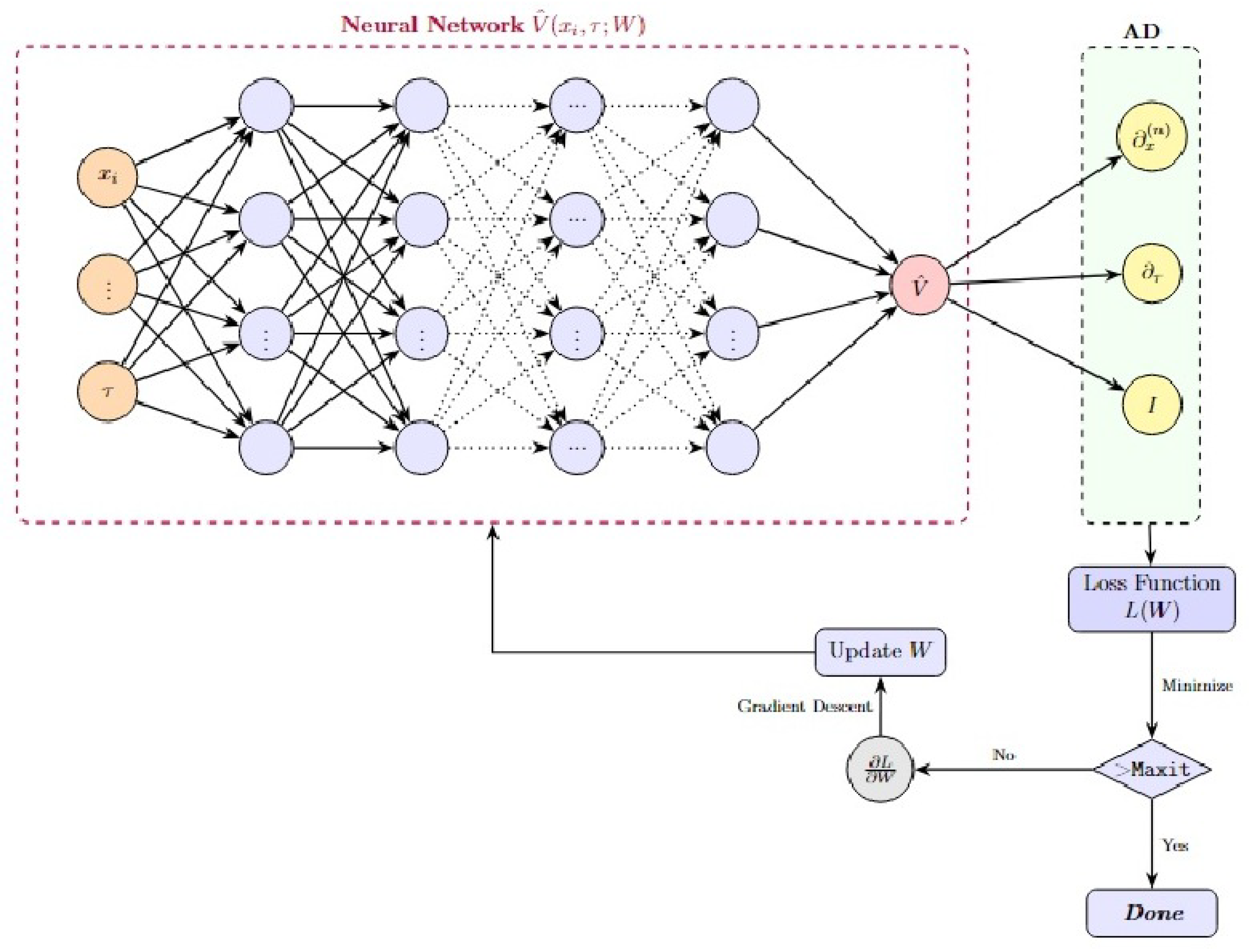
PINNs represent a class of deep learning models that are designed to leverage the structure of governing equations—such as PDEs—along with associated initial and boundary conditions to guide the learning process.
At the core of a PINNs is a neural network , which serves as a function approximator for the solution of the target differential equation, with representing the input vector. The training objective is defined by a composite loss function that encapsulates the system’s physics
- PDE Residual Loss: Enforces the satisfaction of the governing PDE , where denotes the differential operator.
- Boundary Condition Loss: Penalizes deviations from prescribed boundary conditions; .
- Initial Condition Loss: Enforces compliance with initial states of the system.
To compute the necessary derivatives of the neural network for its inputs, PINNs employ automatic differentiation (AD). This eliminates the need for numerical differentiation and enhances the accuracy and stability of gradient computations.
Training is performed by minimising the total loss for the network parameters W using gradient-based optimisation methods. This optimisation process ensures that the neural network solution adheres to the fundamental physical principles encoded in the form of differential equations.
Figure 2.
PINNs Training Scheme for Option Pricing.
To formulate the BSPDE for pricing European options with multiple underlying assets as a PINNs-based problem, we first express the BSPDE in its general form:
subject to boundary conditions:
where is array of with .
Here and are the differential operators on the domain and boundary, respectively. We select (randomly) a collection of interior and boundary points , where each point is in an n-tuple of size (for d=number of stocks and extra one dimension to accommodate time ). The solution of any differential equation using PINNs involves minimizing a single loss function defined as a weighted sum of the norm of the differential equation and boundary conditions:
where and are weights and and are the sets of input points on the domain and boundary, respectively.
Minimizing means we are trying to find a set of weights W for which the PDE, is zero or as close to zero as possible and the boundary conditions are also met, i.e. solves the PDE ([40]).
We use deepxde library of python for our model.
| Algorithm 2 Solving Option Pricing Differential Equations using PINNs |
|
3. Benchmarking: European Call Option on a Single Underlying Asset
As a preliminary validation of our approach, we first consider solving the scaled Black–Scholes partial differential equation (BSPDE) for a single underlying asset. This is achieved by setting in Equation (3):
The scalled price of a European call option, denoted as , is determined by solving Equation (4) subject to the following boundary and initial conditions:
Here, L represents a suitably large truncation parameter, used to approximate the semi-infinite domain by . For computational feasibility, we set .
The input features of one underlying call option are scaled stock price x and time to maturity and one output, the scaled option price (). This problem has a well-known closed-form solution in [37]
For numerical experiments, we solve this model using the following fixed parameter values:
3.1. Supervised Approach for Pricing European Option on Single Asset
For supervised approach we first need to generate a data set. For that, we used uniform distribution to randomly select the stock price (x) ranges from $0.1 to $2.5, and the time to maturity () from 0 years to 1 year. The scaled European call option prices serve as the target values obtained using the analytical solution of the BSPDE.
To implement this approach, we must first determine the appropriate architecture of the neural network, including the number of layers and the number of neurons per layer. The debate over shallow versus deep neural networks has been extensively studied. While increasing the depth of a neural network can enhance accuracy, this comes at the cost of significantly higher computational complexity. Furthermore, as observed by [41], deeper architectures often yield only marginal improvements in accuracy.
We generated 1,000,000 training data points and used them to train a fully connected feedforward neural network with standard hyperparameters (activation function: logistic, solver: L-BFGS,, maximum iterations: 1000). To assess the effect of depth of network, we evaluated models with different numbers of hidden layers and found that a depth of three to seven hidden layers was sufficient. Increasing the number of layers beyond this range did not improve accuracy and, in some cases, led to overfitting, as illustrated in Figure 3.
Similarly, when varying the number of neurons per hidden layer while keeping the number of layers fixed at three, we observed that the optimal performance was achieved with 20–70 neurons per layer. Beyond this range, the accuracy either plateaued or deteriorated due to overfitting, as depicted in Figure 3.
Based on these observations, we selected a neural network architecture with three hidden layers, each containing 30 neurons. Which means our model comprises a total of 7851 trainable parameters.
The next step involved tuning the hyperparameters to achieve optimal performance. The following hyperparameter ranges were considered:
- Activation function: ["logistic", "ReLU", "tanh"]
- Optimizer: ["L-BFGS", "SGD", "Adam"]
- Regularization parameter (): [0.0001, 0.0005, 0.00001]
- Maximum iterations: [1000, 2000, 4000]
We employed the grid search method from the scikit-learn library to identify the optimal hyperparameters. This method evaluates all possible combinations of parameter values and selects the configuration yielding the highest accuracy. The total training time for the grid search procedure was 6991.19 seconds. The optimal hyperparameter configuration was found to be: activation function of ReLU, the solver as Adam, is , and 1000 the maximum number of iterations.
Training the final model on 1,000,000 data points took 264.415 seconds. The model’s performance was evaluated using several key metrics. The root mean squared error (RMSE) was calculated to be 0.0023, indicating a low average deviation between the predicted and actual values. Notably, the RMSE is particularly informative compared to the normalized strike price of $1, as it signifies that the average error constitutes only 0.23% of the strike price. Furthermore, the coefficient of determination () was found to be 99.9999%, demonstrating an exceptional fit between the model’s predictions and the observed data. Additionally, the relative error was determined to be 0.00027, further underscoring the model’s high degree of accuracy. The error is computed using the following equation:
A histogram of the error distribution is shown in Figure 4. The observed error is consistently within , demonstrating the high accuracy of our model.
3.2. Unsupervised Approach (PINNs) for pricing European Option on One Asset
For the PINNs approach, we utilize the equation given in Equation (4), along with the corresponding boundary and initial conditions, as the loss function.
Similar to the supervised approach, we analyze the effect of varying the network depth (number of hidden layers) and width (number of neurons per hidden layer). As expected, increasing these hyperparameters beyond a certain threshold does not lead to significant accuracy improvements, as illustrated in Figure 5. Based on this analysis, we select a PINNs architecture with five hidden layers, each containing 50 neurons. The selected neural network architecture consists of two input nodes and a single output node. This results in a total of 7851 weights.
To determine the optimal number of training iterations and the most effective network structure, we conduct a grid search over the following hyperparameter ranges:
- Activation function: [’ReLU’, ’tanh’, ’swish’, ’sin’, ’sigmoid’]
- Optimizer: ["RMSprop", "SGD", "Adam"]
- Regularization parameter (): [0.0001, 0.0005, 0.00001]
- maximum iterations: [2000, 4000]
We evaluated the loss across all possible parameter combinations and selected the configuration that minimized the error. The optimal hyperparameters obtained from the grid search are: activation function of tanh, solver as Adam, , and a maximum of 3000 iterations.
Training was performed in two stages. Initially, the Adam optimizer was used for 3000 iterations with a learning rate of , Adam achieved a loss of over 16,409.27 seconds. Following this, training switched to the L-BFGS optimizer, which does not require an explicit learning rate, and continued until convergence. L-BFGS attained loss of within 10,236.10 seconds. Overall, the total execution time for the entire training process was approximately 26,673.9 seconds.
To facilitate error comparison, we first convert the PINN-predicted scaled price () into the actual option price () using Equation (2):
To rigorously evaluate the model’s performance, we sample 60,000 random points from the domain . The error is computed using Equation (5), and the resulting error histogram is displayed Figure 6.
The model’s performance was rigorously evaluated using several key metrics. The relative error was calculated to be 0.003156, indicating a minimal discrepancy between the predicted and actual values. The Root Mean Squared Error (RMSE) was determined to be , further demonstrating the model’s precision. Notably, the model achieved an accuracy rate of 100%, underscoring its reliability. Additionally, the coefficient of determination () was found to be 0.99998, signifying an excellent fit and a strong correlation between the model’s predictions and the observed data.
3.3. Comparison of Supervised and Unsupervised Approaches
Table 1 provides a comparative analysis of the two models. The results indicate that PINNs achieve accuracy and efficiency comparable to the supervised, data-driven approach, with slightly higher relative error but competitive RMSE and scores.
4. Pricing Multi-Asset Options Using Neural Networks
Next, we compare the efficiency of supervised and unsupervised neural networks in pricing exchange options with two underlying assets. An exchange option allows the holder to exchange one asset for another, and its price is determined by solving the Black-Scholes PDE for two assets. The governing PDE for such an option is obtained by setting in Equation (3):
defined on . Here, is the correlation coefficient between the two assets. The function is the scaled option value, which depends on the (scaled) prices of the underlying assets and time .
Since exchange options do not have a strike price, we normalise the asset prices by selecting a reasonable scaling factor K. In our case, we define:
and recover the actual option price via:
The payoff function for the scaled exchange option is:
This problem is more complex than standard European options but still admits an exact solution. For numerical experiments, we solve this model using the following fixed parameter values:
In this case, the neural network takes as input the scaled initial prices of the two underlying assets, , along with the time to expiry, . And to calculate the output, From [37], Margrabe’s formula provides the exact solution.
4.1. Supervised Learning Approach for Pricing Exchange Options
To construct the training dataset, we generated random samples from the following uniform distributions:
The initial price of asset one () ranges from $0.1 to $5, while the initial price of asset two () varies between $0.1 and $5. The time to expiry () spans from 0.1 year to 1 year.
The corresponding scaled option prices, , serving as the target values for the model, were computed using the closed-form solution of the Black-Scholes PDE for exchange options.
We trained a fully connected neural network comprising of four hidden layers, each containing 40 neurons. The depth and width were decided using the discussion in the single asset case. To optimize the neural network architecture, we performed a comprehensive grid search over a range of hyperparameters described in the last section. This process, which took approximately 9,738.35 seconds, identified the following optimal configuration: the activation function employed was Rectified Linear Unit (ReLU); the optimization algorithm utilized was Adam; the regularization parameter () was set to ; and the maximum number of iterations allowed was 1000.
With these parameters, The training process, conducted on a dataset of 1,000,000 samples, was completed in 233.23 seconds. The model demonstrated exceptional accuracy, achieving a root-mean-squared error (RMSE) of 0.00095 and an R² score of 99.9999%, indicating near-perfect alignment with the exact solution. Additionally, the L2 relative error was found to be 0.00067, further affirming the model’s precision.
Figure 7 illustrates the distribution of errors. The histogram exhibits a bell-shaped curve, centered around zero, with error values constrained within , underscoring the robustness and reliability of the model’s predictions.
4.2. Pricing Exchange Options Using Physics-Informed Neural Networks
To price exchange options using Physics-Informed Neural Networks (PINNs), we use the PDE given in Equation (6), as the loss function of the neural network, along with appropriate boundary and initial conditions. The option pricing parameters are identical to those used in the previous section for consistency and comparability.
The spatial domain is truncated to a bounded computational region, where and . The imposed Dirichlet boundary conditions ensure numerical stability and accurate representation of the problem physics. Specifically, the option price is set to zero at the boundaries and , i.e.,
Additionally, at (maturity) or when , the payoff condition follows the exchange option structure: We decided the neural network to have a fully connected architecture with a depth of six layers, including five hidden layers, each with 40 neurons, resulting in a total of 3,871 trainable parameters. The discussion in the case of single asset provides us with a reasonable range to choose depth and width from.
The optimal hyperparameters identified using gridsearch, were a sine activation function, the Adam optimizer as the solver, a regularization parameter () of , and a maximum of 4000 iterations. The training dataset comprised 20,000 residual points sampled within the spatio-temporal domain, 2,000 training points sampled on the boundary, and 1,000 residual points corresponding to the initial conditions.
The training process was conducted in two phases. Initially, the Adam optimizer was employed which achieved a final training loss of in approximately 3,505.2 seconds. Followed by a switch to the L-BFGS optimizer which further reduced the training loss to over an additional 15,757.1 seconds. The total training time for both optimizers was 19,262.3 seconds. This two-stage optimization approach ensured robust convergence and minimized the residual error in the PINN-based solution.
Figure 8 shows the 3d plot of numerical solution of exchange option using PINNS at .
To rigorously assess the performance of our Physics-Informed Neural Network (PINN) model, we sampled 60,000 random points from the input domain. The resulting error histogram, depicted in Figure 8, exhibits a bell-shaped distribution centered around zero, with errors confined within , indicating minimal deviation.
Quantitative evaluation metrics further substantiate the model’s efficacy: the L2 relative error was computed to be 0.0106, and the root mean square error (RMSE) was determined to be . Moreover, the model achieved an accuracy rate of 100%, and the coefficient of determination () was calculated as 0.9998, signifying an excellent
4.3. Comparison of Supervised & Unsupervised Approach
Table 2 shows a comparison of the two models.
5. Conclusions
This investigation provides a comprehensive comparative analysis of supervised neural networks and Physics-Informed Neural Networks (PINNs) in the context of multi-asset option pricing, with a particular emphasis on exchange options. Notably, our study introduces the application of grid search methodologies for hyperparameter optimization within this domain—a technique seldom employed in option pricing models utilizing neural networks. This approach enabled a systematic exploration of neural network architectures, including an in-depth examination of network depth and width, which represents a novel contribution to option pricing research.
Empirical evidence from our study indicates that supervised learning models, which leverage extensive market datasets, exhibit remarkable efficiency in both computational speed and predictive accuracy. This efficiency renders them highly suitable for real-time financial applications where rapid decision-making is critical.
Conversely, PINNs emerge as a potent alternative in environments characterized by limited or non-existent market data. By embedding the fundamental partial differential equations governing option pricing directly into the neural network’s loss function, PINNs provide a robust framework capable of tackling intricate pricing challenges without the necessity for large datasets. This intrinsic incorporation of domain-specific knowledge enables PINNs to maintain predictive reliability even in data-scarce scenarios.
The outcomes of this study underscore the importance of aligning the choice of modelling technique with data availability and the specific demands of the financial application at hand. Future research endeavours could explore the development of hybrid models that synergistically combine the strengths of both supervised learning and PINNs. Additionally, extending the application of these methodologies to more complex derivative instruments and diverse market conditions could significantly enhance the repertoire of tools available for financial modelling. Such advancements would further solidify the integration of machine learning techniques within the domain of quantitative finance, offering more versatile and resilient modelling approaches.
Funding
This research received no external funding.
Conflicts of Interest
The authors declare no conflicts of interest.
References
- Horváth, Á.; Medvegyev, P. Pricing Asian Options: A Comparison of Numerical and Simulation Approaches Twenty Years Later. ERN: Options (Topic) 2016. Available online: https://api.semanticscholar.org/CorpusID:31807417.
- Turnbull, S.; Wakeman, L. A Quick Algorithm for Pricing European Average Options. J. Financ. Quant. Anal. 1991, 26, 309–326. [CrossRef]
- Levy, E. The Valuation of Average Rate Currency Options. J. Int. Money Finance 1992, 11, 474–491. [CrossRef]
- Geman, H.; Yor, M. Bessel Processes, Asian Options, and Perpetuities. Math. Finance 1993, 3, 349–375. [CrossRef]
- Kirkby, J.L. An Efficient Transform Method for Asian Option Pricing. SIAM J. Financ. Math. 2016, 7, 845–892.
- Kemna, A.G.Z.; Vorst, A.C.F. A Pricing Method for Options Based on Average Asset Values. J. Bank. Finance 1990, 14, 113–129.
- Rumelhart, D.; Hinton, G.; Williams, R. Learning Representations by Back-Propagating Errors. Nature 1986, 323, 533–536.
- Vecer, J. Unified Asian Pricing. Risk 2002, 15, 113–118.
- Boyle, P.P.; Evnine, J.; Gibbs, S. Numerical Evaluation of Multivariate Contingent Claims. Rev. Financ. Stud. 1989, 2, 241–250.
- Boyle, P.P. Options: A Monte Carlo Approach. J. Financ. Econ. 1977, 4, 323–338. [CrossRef]
- Broadie, M.; Glasserman, P. Estimating Security Price Derivatives Using Simulation. Manag. Sci. 1996, 42, 269–285. [CrossRef]
- Courtadon, G. A More Accurate Finite Difference Approximation for the Valuation of Options. J. Financ. Quant. Anal. 1983, 17, 697–703. [CrossRef]
- Cox, J.C.; Ross, S.A.; Rubinstein, M. Option Pricing: A Simplified Approach. J. Financ. Econ. 1979, 7, 229–263. [CrossRef]
- Culkin, R. Machine Learning in Finance: The Case of Deep Learning for Option Pricing. Comput. Sci. 2017. Available online: https://api.semanticscholar.org/CorpusID:92991481.
- Dilloo, M.J.; Tangman, D.Y. A High-Order Finite Difference Method for Option Valuation. Comput. Math. Appl. 2017, 74, 652–670. [CrossRef]
- Eskiizmirliler, S.; Günel, K.; Polat, R. On the Solution of the Black-Scholes Equation Using Feed-Forward Neural Networks. Comput. Econ. 2021, 58, 915–941. [CrossRef]
- Black, F.; Scholes, M. The Pricing of Options and Corporate Liabilities. J. Polit. Econ. 1973, 81, 637–654. [CrossRef]
- Garcia, R.; Gençay, R. Pricing and Hedging Derivative Securities with Neural Networks and a Homogeneity Hint. J. Econom. 2000, 94, 93–115. [CrossRef]
- Gatta, F.; Schiano Di Cola, V.; Giampaolo, F.; Piccialli, F.; Cuomo, S. Meshless Methods for American Option Pricing through Physics-Informed Neural Networks. Eng. Anal. Bound. Elem. 2023, 151, 68–82. [CrossRef]
- Han, J.; Jentzen, A.; Ee, W. Solving High-Dimensional Partial Differential Equations Using Deep Learning. Proc. Natl. Acad. Sci. 2018, 115, 8505–8510. [CrossRef]
- Hozman, J.; Tichý, T. DG Method for Numerical Pricing of Multi-Asset Asian Options—The Case of Options with Floating Strike. Appl. Math. 2017, 62, 171–195. [CrossRef]
- Hutchinson, J.M.; Lo, A.W.; Poggio, T. A Nonparametric Approach to Pricing and Hedging Derivative Securities via Learning Networks. J. Finance 1994, 49, 851–889.
- Kaya, D. Pricing a Multi-Asset American Option in a Parallel Environment by a Finite Element Method Approach. Ph.D. Thesis, Uppsala University, Uppsala, Sweden, 2011. https://urn.kb.se/resolve?urn=urn:nbn:se:uu:diva-155546.
- Koffi, R.S.; Tambue, A. A Fitted L-Multi-Point Flux Approximation Method for Pricing Options. Comput. Econ. 2022, 60, 633–663. https://api.semanticscholar.org/CorpusID:209516245.
- Liao, W.; Khaliq, A.Q.M. High-Order Compact Scheme for Solving Nonlinear Black–Scholes Equation with Transaction Cost. Int. J. Comput. Math. 2009, 86, 1009–1023. [CrossRef]
- Longstaff, F.A.; Schwartz, E.S. Valuing American Options by Simulation: A Simple Least-Squares Approach. Rev. Financ. Stud. 2001, 14, 113–147. http://dx.doi.org/10.1093/rfs/14.1.113.
- Andalaft-Chacur, A.; Ali, M.M.; Salazar, J.G. Real Options Pricing by the Finite Element Method. Comput. Math. Appl. 2011, 16, 2863–2873. [CrossRef]
- McCulloch, W.S.; Pitts, W. A Logical Calculus of the Ideas Immanent in Nervous Activity. Bull. Math. Biophys. 1943, 5, 115–133. Reprinted in McCulloch, 1964, pp. 16–39. [CrossRef]
- Mollapourasl, R.; Fereshtian, A.; Vanmaele, M. Radial Basis Functions with Partition of Unity Method for American Options with Stochastic Volatility. Comput. Econ. 2019, 53, 259–287. [CrossRef]
- Moon, K.-S.; Kim, W.-J.; Kim, H. Adaptive Lattice Methods for Multi-Asset Models. Comput. Math. Appl. 2008, 56, 352–366. [CrossRef]
- Ruf, J.; Wang, W. Neural Networks for Option Pricing and Hedging: A Literature Review. J. Comput. Financ. 2020, 24, 1–45. [CrossRef]
- Seydel, R.U. Tools for Computational Finance, 5th ed.; Springer: Berlin, Germany, 2012.
- Sola, J.; Sevilla, J. Importance of Input Data Normalization for the Application of Neural Networks to Complex Industrial Problems. IEEE Trans. Nucl. Sci. 1997, 44, 1464–1468. [CrossRef]
- Soleymani, F.; Zhu, S. RBF-FD Solution for a Financial Partial-Integro Differential Equation Utilizing the Generalized Multiquadric Function. Comput. Math. Appl. 2021, 82, 161–178. [CrossRef]
- Wang, S.; Zhang, S.; Fang, Z. A Superconvergent Fitted Finite Volume Method for Black-Scholes Equations Governing European and American Option Valuation. Numer. Methods Partial Differ. Equ. 2014, 31, 1190–1208. [CrossRef]
- Wang, X.; Li, J.; Li, J. A Deep Learning Based Numerical PDE Method for Option Pricing. Comput. Econ. 2023, 62, 149–164. [CrossRef]
- Wilmott, P. Paul Wilmott on Quantitative Finance, 2nd ed.; John Wiley and Sons: Hoboken, NJ, USA, 2006.
- Wilmott, P.; Dewynne, J.; Howison, S. Option Pricing: Mathematical Models and Computation; Oxford Financial Press: Oxford, UK, 1993.
- Du Toit, J.F.; Laubscher, R. Evaluation of Physics-Informed Neural Network Solution Accuracy and Efficiency for Modeling Aortic Transvalvular Blood Flow. Math. Comput. Appl. 2023, 28, 62. [CrossRef]
- Lu, L.; Meng, X.; Mao, Z.; Karniadakis, G.E. DeepXDE: A Deep Learning Library for Solving Differential Equations. SIAM J. Sci. Comput. 2019, 41, A463–A483. [CrossRef]
- Zagoruyko, S.; Komodakis, N. Wide Residual Networks. In Proceedings of the British Machine Vision Conference (BMVC); 2016. [CrossRef]
- Ahmad, A.; Khan, A. Pricing Rainbow Options Using PINNs. Preprints 2024, August. License CC BY 4.0. Institution: Adnan Khan’s Lab. [CrossRef]
Figure 3.
Impact of depth and width of neural network on supervised learning problem.(a) shows Effect of the number of layers on error while (b) shows Effect of the number of neurons per layer on error.
Figure 3.
Impact of depth and width of neural network on supervised learning problem.(a) shows Effect of the number of layers on error while (b) shows Effect of the number of neurons per layer on error.
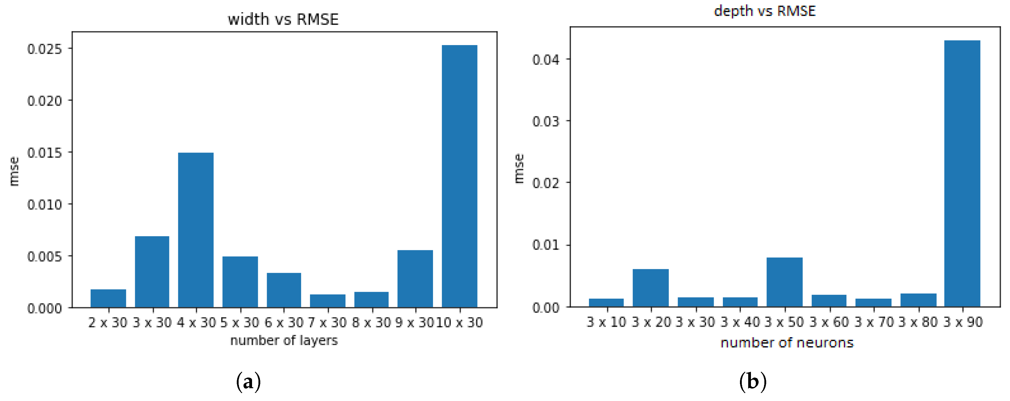
Figure 4.
one underlying option priced using supervised neural network.
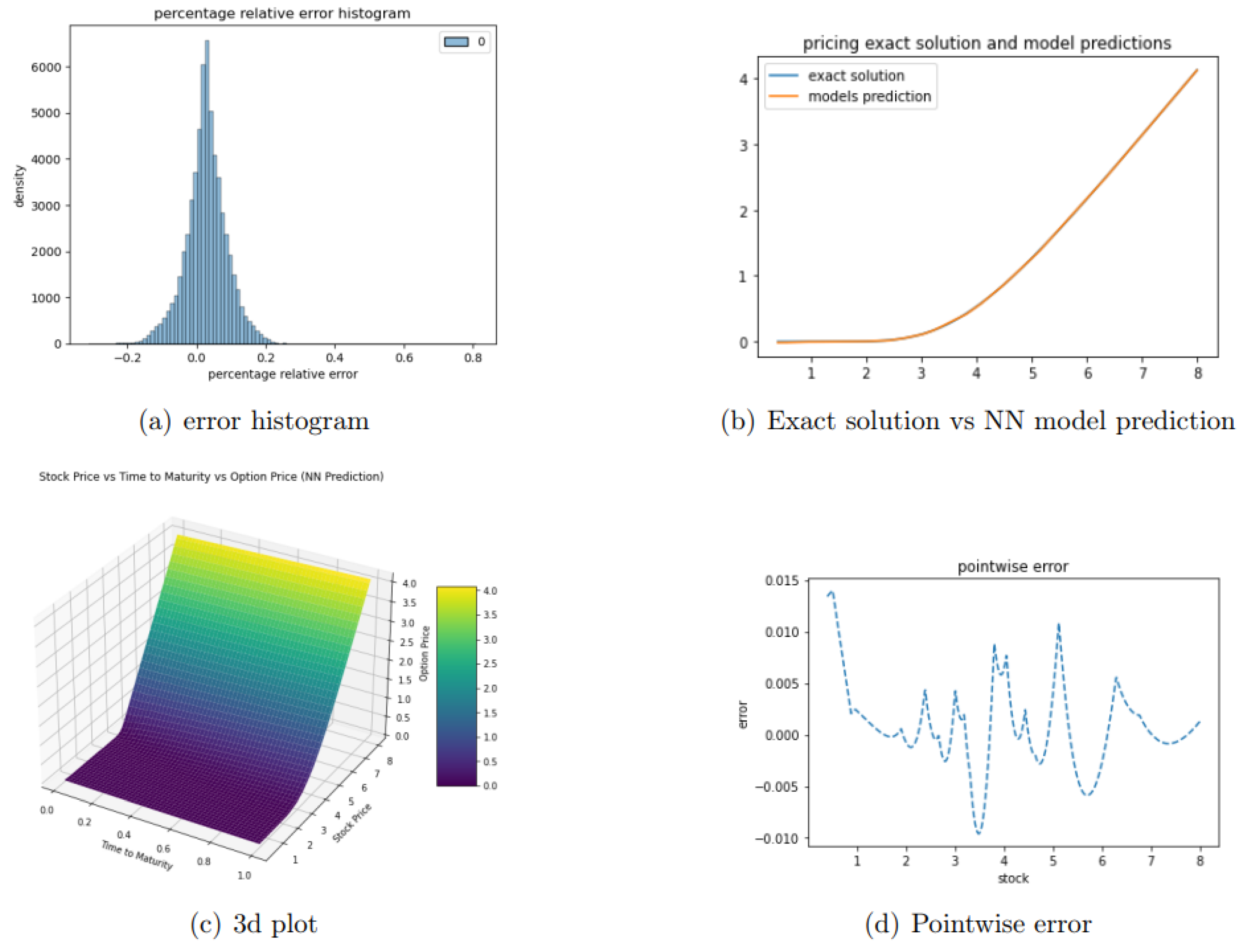
Figure 5.
Impact of network depth and width on PINN accuracy for pricing a European option. (a) shows Effect of number of hidden layers on error, (b) shows Effect of number of neurons per layer on error
Figure 5.
Impact of network depth and width on PINN accuracy for pricing a European option. (a) shows Effect of number of hidden layers on error, (b) shows Effect of number of neurons per layer on error
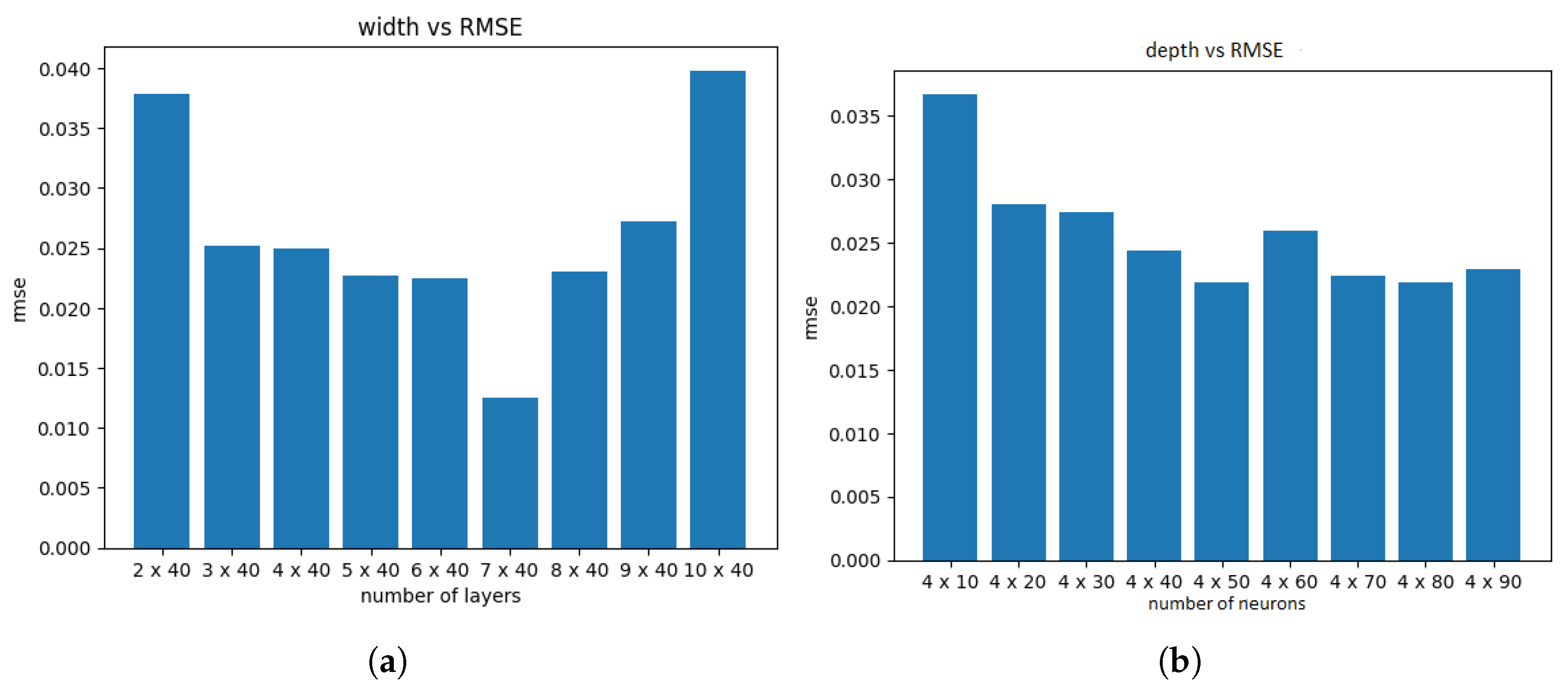
Figure 6.
one underlying option priced using PINNs.
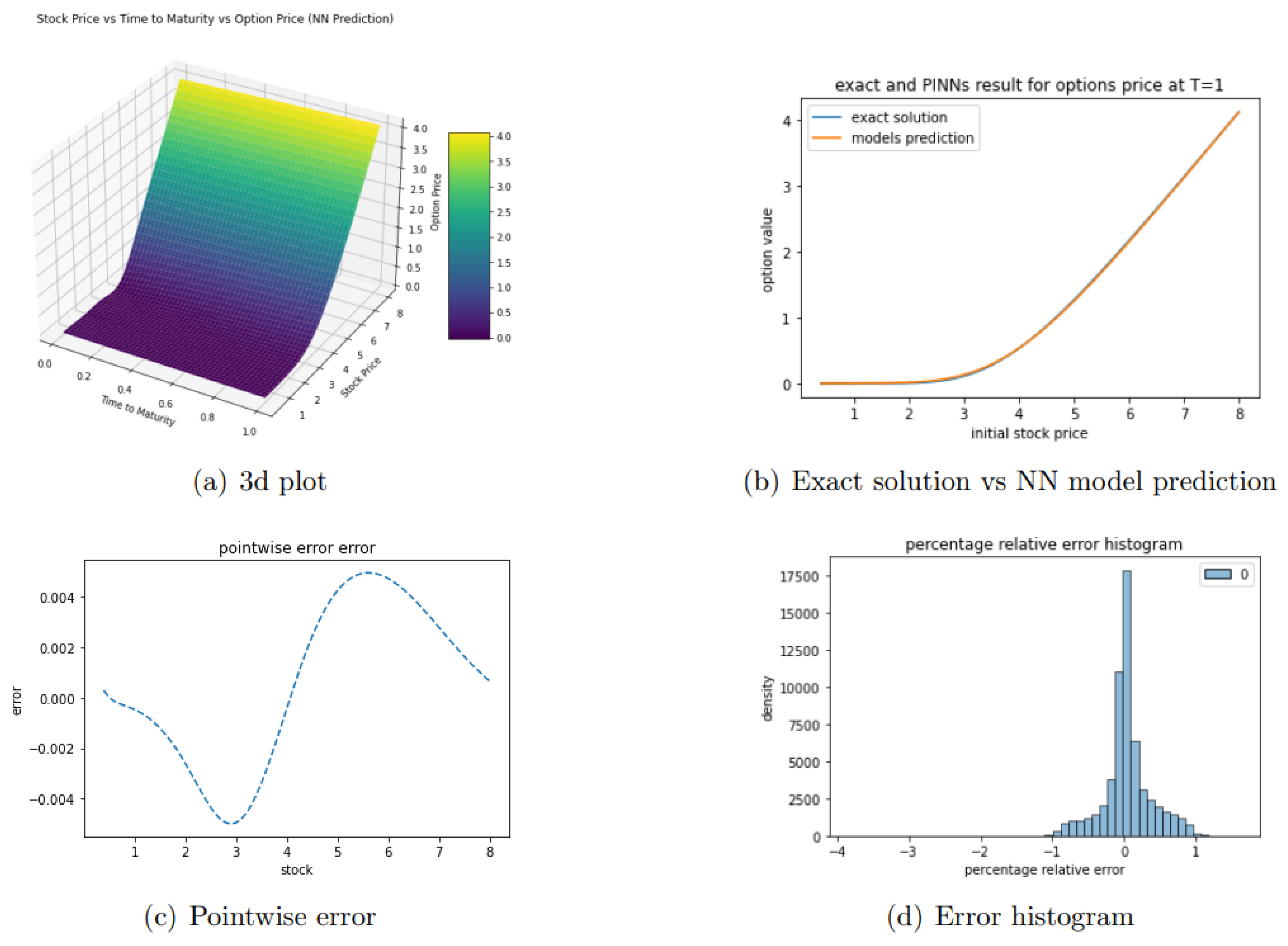
Figure 7.
two-asset exchange option, priced using Supervised Approach. (a)3d plot of exchange option at time to expiry one, (b) relative percentage error histogram.
Figure 7.
two-asset exchange option, priced using Supervised Approach. (a)3d plot of exchange option at time to expiry one, (b) relative percentage error histogram.
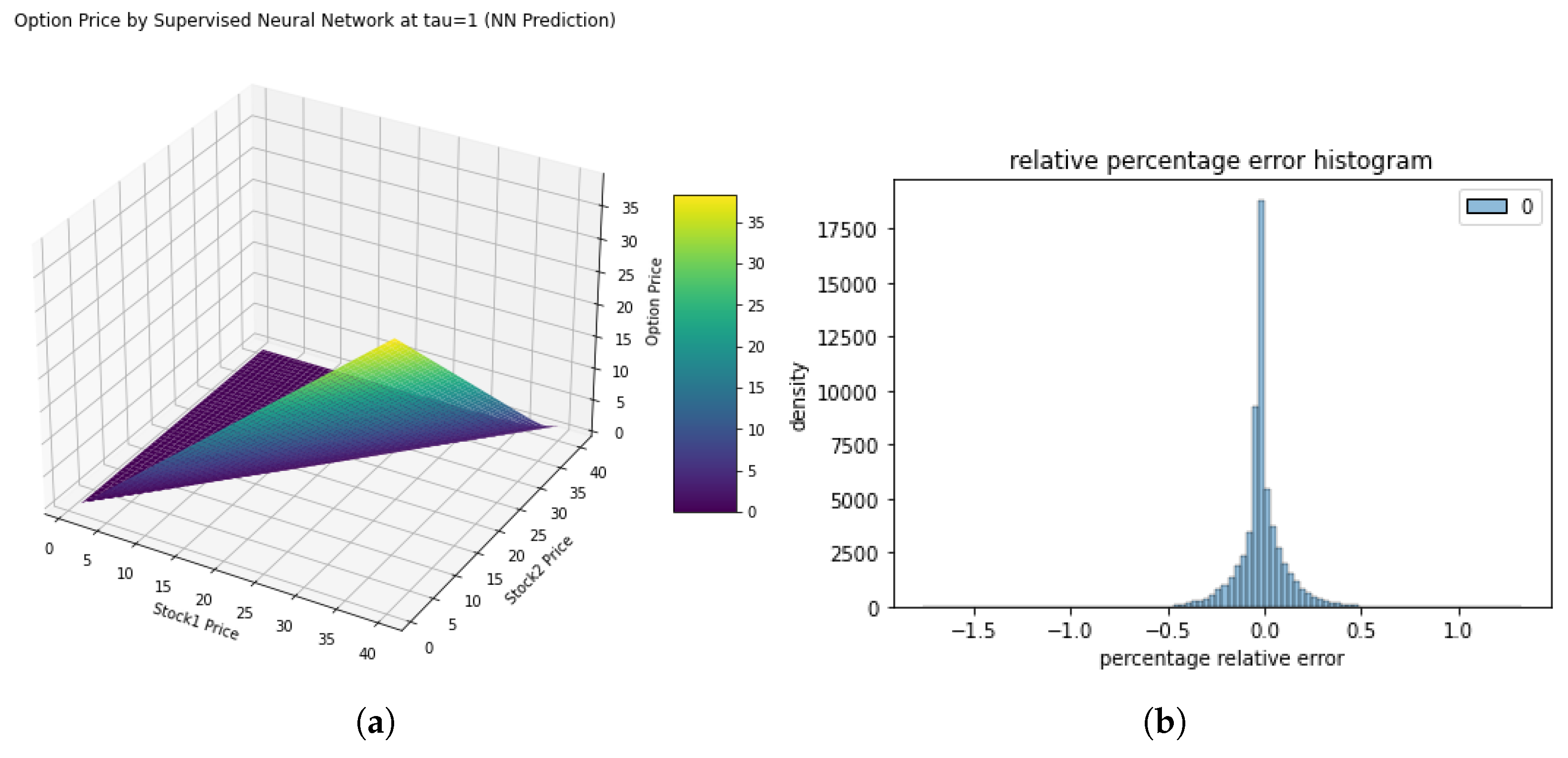
Figure 8.
two-asset exchange option, priced using PINNs. (a)3d plot of exchange option at time to expiry one, (b) relative percentage error histogram.
Figure 8.
two-asset exchange option, priced using PINNs. (a)3d plot of exchange option at time to expiry one, (b) relative percentage error histogram.
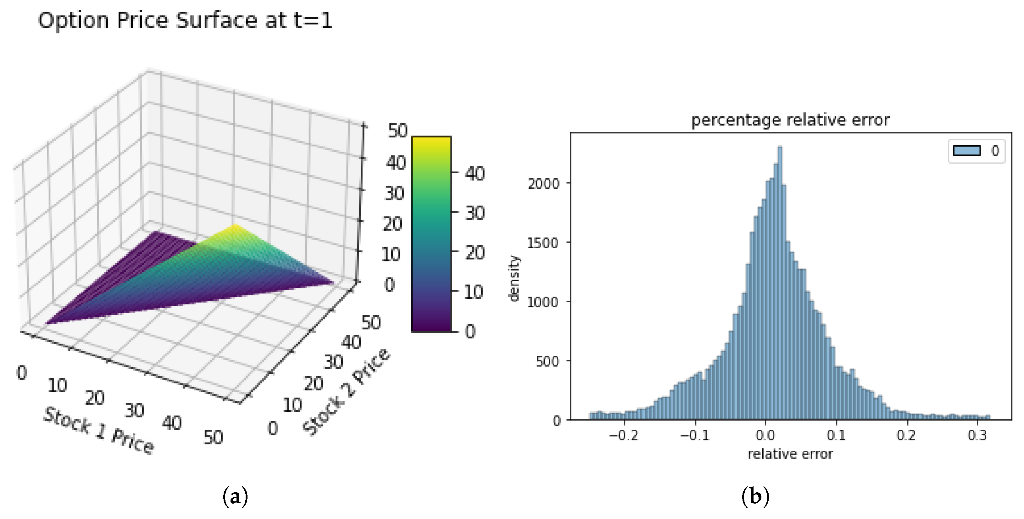

Table 1.
Performance Comparison of Supervised Learning and PINNs
| Metric | Supervised Approach | PINNs |
|---|---|---|
| RMSE | ||
| Score | ||
| Relative Error | ||
| Accuracy (%) |
Table 2.
Model Performance Comparison for exchange options
| Metric | Supervised Approach | PINNs |
|---|---|---|
| RMSE | ||
| R² score | ||
| L2 relative error | ||
| Accuracy (%) | 100% | 100% |
Disclaimer/Publisher’s Note: The statements, opinions and data contained in all publications are solely those of the individual author(s) and contributor(s) and not of MDPI and/or the editor(s). MDPI and/or the editor(s) disclaim responsibility for any injury to people or property resulting from any ideas, methods, instructions or products referred to in the content. |
© 2025 by the authors. Licensee MDPI, Basel, Switzerland. This article is an open access article distributed under the terms and conditions of the Creative Commons Attribution (CC BY) license (https://creativecommons.org/licenses/by/4.0/).
Copyright: This open access article is published under a Creative Commons CC BY 4.0 license, which permit the free download, distribution, and reuse, provided that the author and preprint are cited in any reuse.


