Production Planning for Manufacturing of Car Parts

1. Production Planning

Production planning in a factory or any organization is essential. This necessity is so critical in some cases that its absence can lead to significant damage. Production planning is closely related to the organization’s core processes, such as production, sales, procurement, and warehousing. These complex interactions make the planning unit always concerned about meeting customer demands [1]. Scheduling and sequencing operations in production planning play a critical and influential role in the success of any manufacturing organization. Effective production scheduling prevents capital buildup, reduces waste, minimizes or eliminates machine downtime, and strives for better utilization of machinery. It also ensures timely responses to customer orders and provides raw materials and parts at the right time [2]. Production scheduling aims to allocate limited resources over time to carry out a group of activities. Having an appropriate production schedule significantly impacts the efficiency and achievement of organizational goals. The production scheduling model in each manufacturing organization varies according to its goals and priority access. Therefore, the goals, priorities, and resource constraints must first be examined to determine a suitable scheduling model in an organization. Production planning is essentially about scheduling and determining the optimal sequence of tasks. Clearly, for a manufacturing unit, minimizing costs and increasing productivity are of great importance. Thus, scheduling in terms of numbers, time, and location is necessary to minimize costs and increase productivity. Currently, most factories operate without using scientific production planning methods, leading to issues such as various production interruptions, lack of forecasting for required raw materials, insufficient production time, and inability to decide on the production mix. Modeling allows managers to optimize the production process in terms of time and cost, thereby increasing production efficiency. Solving production issues through quantitative models not only provides optimal solutions for the current production status but also helps planners answer "what if..." questions. Answering such questions through experiential and practical means can be costly and, in many cases, impossible. The necessity of planning is evident to all, and specifically, planning in the production process has such advantages that its absence can deviate manufacturing organizations from the path of healthy growth and continued survival in a competitive environment. In this regard, planning helps also mitigate the uncertainties raised from the demand side. Usually, mixed-integer programming models are leveraged to maximize the revenue of companies (e.g., [3,4]). However, these models are vastly applied in production planning and scheduling too [2,5]. The central aim of this research is to create a unified production planning framework that integrates both Aggregate Production Planning (APP) and Master Production Scheduling (MPS) through an innovative MILP model. The key goal is to reduce the overall costs linked to production, inventory storage, and setup processes across a six-month planning period. Key assumptions underpinning our model include the prohibition of shortages, fixed labor levels without hiring or layoffs, and the consideration of opportunity costs as the sole inventory holding costs. The integrated planning approach ensures that production planning for both product families and individual products is conducted concurrently, with distinct planning horizons and periods for APP and MPS. Specifically, APP is executed every month over a six-month horizon, while MPS operates every week over a two-month horizon. This paper is structured as follows: We begin by detailing the mathematical formulation of our integrated production planning model, followed by a discussion of the parameters, indices, and decision variables used in the model. Subsequently, we present the results obtained from solving the model and compare these results with the current operational data from the company’s accounting department. Finally, we conclude with an analysis of the benefits of our hierarchical production planning approach, highlighting its potential for significant cost savings and operational efficiency improvements.

2. Related Work

The field of production planning and scheduling has a rich history, marked by significant advancements and the development of various methodologies. The origins of modern production planning can be traced back to [6] seminal work on the Economic Order Quantity (EOQ) model, which laid the foundation for inventory management and production planning in manufacturing systems. Over the decades, this foundational work has been expanded upon, leading to the development of more sophisticated and integrated planning models [7,8]. In the early 1960s, Material Requirements Planning (MRP) emerged in the United States as a computerized approach to planning the procurement and production of materials. A comprehensive manual on this approach was published by [9]. Undoubtedly, MRP techniques were utilized manually and in a hybrid manner in various parts of Europe before World War II. However, [9] realized that computers could incorporate all the details of the MRP technique, making it highly effective for managing work-in-progress inventories. The initial plan for computerizing MRP was based on a Bill of Materials Processor (BOMP). This processor translated the production schedule of parent items into production or procurement schedules for component items. This method, referred to as "exploding" the product requirements down the Bill of Materials (BOM), identified the demand for individual parts. corporations. Over time, the adoption of these systems spread to various companies, with additional operational features being integrated into the software to improve their effectiveness. Enhancements to the original system included the addition of the Master Production Schedule (MPS), Production Activity Control (PAC), Rough-Cut Capacity Planning (RCCP), Capacity Requirements Planning (CRP), and Purchasing functionalities. MRP approach was further enhanced by [10] with the introduction of Manufacturing Resource Planning (MRP II), which extended MRP to include additional resources such as labor and machine capacity. The concept of hierarchical production planning was introduced by [11], who proposed a structured approach to integrating production planning and scheduling across different organizational levels. This approach was later elaborated upon by [12], who emphasized the importance of hierarchical integration in achieving efficient production planning. [13] stated that the integration of planning modules such as CRP, MRP, and MPS with execution modules like PAC and Purchasing, coupled with the establishment of feedback loops from execution to planning, led to the development of a more advanced form of MRP, known as Closed-Loop MRP. By incorporating specific financial modules into the Closed-Loop MRP, expanding the Master Production Schedule to serve as the primary or reference plan, and providing support for business planning from a financial standpoint, a comprehensive system was created. The success of MRP implementation was strongly linked to management’s commitment and the training of all production personnel. Consequently, the emphasis on optimization techniques derived from operations research and management science gradually declined. The message repeatedly conveyed was that real issues in industries were related to order, training, understanding, and communications (not numerical and optimization issues). This message, promoted by APICS, was echoed by a large number of consultants and repeated by the computer industry, which was keen on expanding its application. One of the key factors contributing to the widespread adoption of MRP as a production management technique was its ability to leverage computer capabilities to store and access vast amounts of information, which was crucial for the efficient operation of any company. Moreover, the MRP system facilitated the coordination of various activities, including engineering, production, and materials management, within the production unit. Consequently, the attractiveness of MRP II stemmed not only from its function as a decision-support tool for management but, more importantly, from its role as an integrator within the manufacturing organization. Today, there are considerations about how to integrate MRP-type systems with Computer-Integrated Manufacturing (CIM) environments and the adequacy of such systems compared to alternative production philosophies like Just-In-Time (JIT) and proprietary techniques like Optimized Production Technology (OPT). Repeated failures in achieving the promised benefits of these systems have raised multiple questions about the effectiveness of MRP. The Theory of Constraints (TOC), introduced by [14] provided a new perspective on production planning by focusing on identifying and managing bottlenecks within the production process. This theory has been instrumental in developing scheduling techniques that optimize throughput and reduce production lead times. In recent years, the application of advanced mathematical and computational techniques has further refined production planning and scheduling models. For instance, [15] developed a scheduling model specifically for mold injection molding production, addressing the unique challenges of this manufacturing process. [16] applied genetic algorithms to solve flexible job-shop scheduling problems, demonstrating the effectiveness of heuristic methods in complex production environments. [17] introduced a tactical planning model for job shops, which provided a framework for integrating production planning with operational scheduling. [5] offered a comprehensive overview of scheduling theory, algorithms, and systems, highlighting the advances in deterministic and stochastic scheduling models. These foundational works and subsequent advancements have shaped the current production planning and scheduling landscape. As explored in this paper, the integration of hierarchical planning models builds upon these established methodologies, offering a comprehensive approach to optimizing production processes in a manufacturing environment. [18] focused on the critical issue of water scarcity in agricultural supply chains, a topic that had not been extensively explored in the literature. To address this gap, they proposed a hybrid model that integrates optimized neural networks with meta-heuristic algorithms and mathematical optimization to create a sustainable agricultural supply chain. Moreover, machine learning has significant potential in supply chains and production planning. For a recent literature review see [8,19,20,21,22].

In this paper, production planning based on the MRP II approach is considered, which hierarchically includes the following four phases and stages.

2.1. The Logic of MRP and the Four Phases of Production Planning

2.1.1. Aggregate Production Planning (APP)

Aggregate Production Planning is the process of preparing a production plan over a medium-term horizon (three months to one year). This plan specifies the optimal combination of production levels, inventory levels, overtime, and labor requirements at the aggregate product level, broken down by aggregate periods (at least monthly). The goal is to meet the forecasted demand for products over the planning horizon in the most cost-effective manner. The objective of APP is to create a medium-term production plan to utilize available resources to meet the variable forecasted demands. In this type of planning, final sellable products are combined into aggregate products (types or families of products) for various reasons, and planning is done at this aggregate product level, serving as the basis for creating the production plan for final products. For a recent literature review see [23].

2.1.2. Master Production Schedule (MPS)

The Master Production Schedule is the production plan for final products over a shorter time horizon compared to Aggregate Production Planning (one to three months). Its main input is the forecasted demand at the level of final products. An effective MPS provides principles for accepting new customer orders, efficiently utilizing limited resources, achieving the strategic objectives specified in the production plan, and balancing production and sales. At an operational level, the most crucial decision-making issue is the preparation and updating of the MPS. In MPS, the aggregate production plan is converted into an executable production plan at the level of sellable final products, broken down into shorter periods (weekly), see [24].

2.1.3. Material Requirements Planning (MRP)

The master production schedule for finished products must be translated into a production or procurement plan for the raw materials required to assemble these products. Material Requirements Planning (MRP) operates on the principle that manufacturing final products often necessitates several components or subassemblies, with their demand being directly linked to the demand for the final products. As a result, careful planning is essential to ensure that the necessary components and subassemblies are available in a timely and sufficient manner. An MRP system is vital for material planning and control, as it transforms the master production schedule into production plans for make-to-stock components and procurement plans for buy-to-stock materials and components, see [25].

2.1.4. Scheduling

This phase determines the sequence of tasks in workshops and on machines. This is the most detailed and executable stage of production planning, see [26].

2.1.5. Production System of the Company

The company’s production system is Make-to-Stock (MTS). This means production takes place, items are stored in inventory, and orders are fulfilled from the inventory stock. For production planning, an initial six-month horizon is considered. The sales department evaluates the market every six months and provides a forecast report to the production planning unit. Production is divided based on machine capacity, labor hours, future sales forecasts, and so on, resulting in monthly, weekly, and daily production plans. The production plan in this factory is monthly, and besides the six-month report, a report is also received from the sales unit every month.

2.1.6. Diagnostic Analysis

Diagnostic analysis involves identifying existing problems in the company and providing appropriate and practical solutions to address them. Based on the research conducted, several factors hindering productivity improvement were identified, including financial, organizational, structural, planning, governmental regulations, and technical issues.

Some of the technical problems include:

• Low quality of products and services
• Difficulty in procuring raw materials on time for production
• Very low utilization of assets
• Lower production levels compared to nominal capacity for various reasons

3. Problem Definition

This paper deals with the production planning of multiple automotive parts for the Tawana Sanat Akam Company over a medium-term horizon of 6 months. To transform a general planning problem into models with hierarchical levels, we first need to identify the related planning and production activities.

Based on this premise, we have divided the products of this factory as follows:

Row	1	2	3	4	5
Products	Front Heater Case	Lower and Upper Armrest Case	Door Bumpers	Heater Air Distribution Vent	Upper Air Conditioner and Heater Case
Family Number	1	2	3	4	5

Each product manufactured in this factory has its production process, and it does not seem easy to draw all these processes for this project. Given the assumptions of hierarchical planning modeling presented in the next phase, we only consider the bottleneck stage. For instance, we will show the production process of the Lower and Upper Armrest covers for the car:

Figure 1. A picture of the product.

Figure 1. A picture of the product.

Figure 2. Diagram of the tree of the product

Figure 2. Diagram of the tree of the product

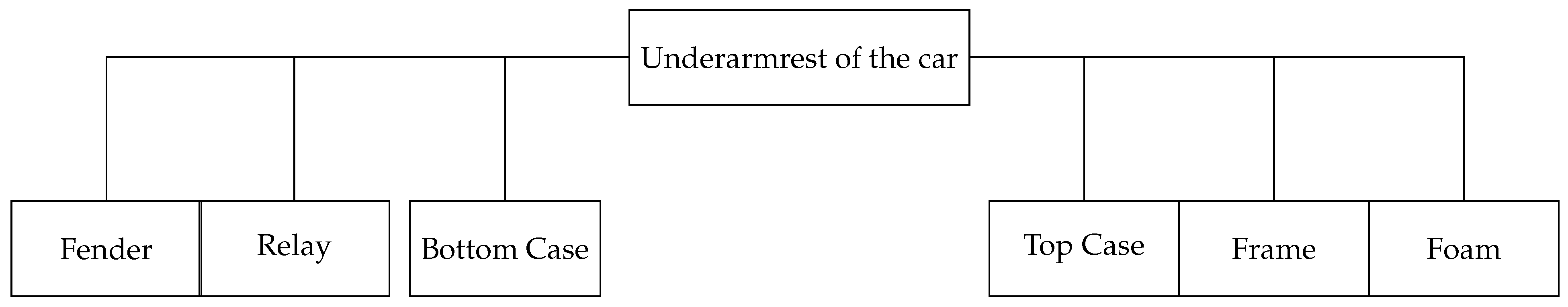
Figure 3. The diagram of the operations process

Figure 3. The diagram of the operations process

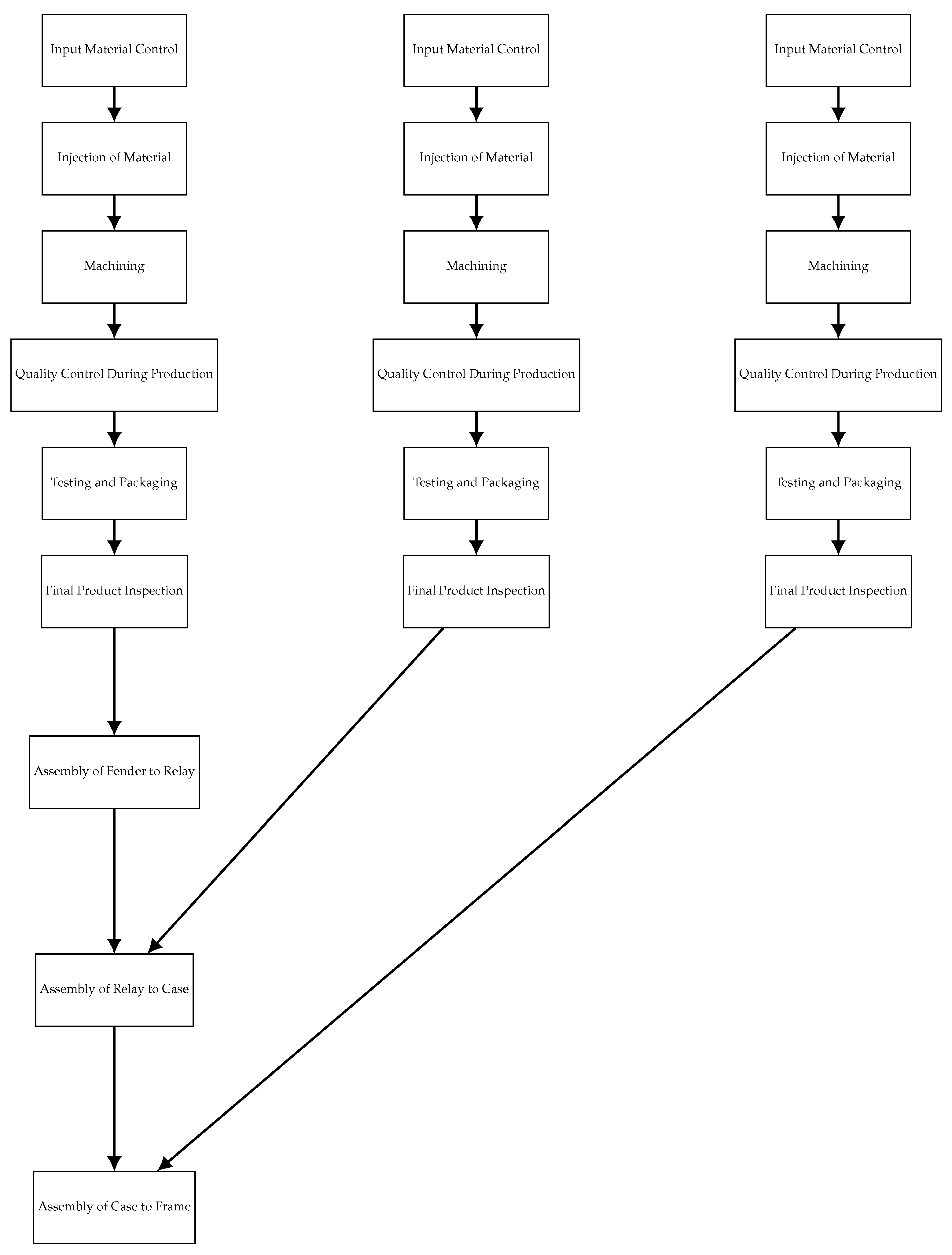
Considering that most of the company’s products use the same plastic injection machines, the bottleneck stage for all products is essentially the plastic injection stage. This modeling aims to optimize all costs, including production and storage, to achieve the minimum total cost of production over a 6-month horizon.

Problem Assumptions:

• Shortages are not allowed, and any inability to meet demand will result in lost sales with very high costs.
• The labor force level is fixed, with no hiring or firing.
• Storage costs are fixed, and only opportunity costs are considered as holding costs for products in inventory.
• MPS and AP planning are only performed for the bottleneck stage, which is the plastic injection section.

4. Mathematical Modeling

For modeling, we use an integrated planning approach. In this approach, production planning for both the family of products and the final products is carried out simultaneously. However, the planning horizon and periods at the AP level are longer than those at the MPS model level. For example, an aggregated production plan might be created for a six-month horizon with monthly planning periods, while the final products’ production plan might be prepared for a two-month horizon with weekly planning periods. Thus, the integrated model for simultaneous AP and MPS planning is written as follows:

Table 1. Indices

Symbol	Values	Definition
P	$1,2,3,\dots ,P$	Aggregated period
I	$1,2,3,\dots ,N$	Product family
t	$1,2,\dots ,4P$	Non-aggregated period

Table 1. Indices

Symbol	Values	Definition
P	$1,2,3,\dots ,P$	Aggregated period
I	$1,2,3,\dots ,N$	Product family
t	$1,2,\dots ,4P$	Non-aggregated period

Table 2. Parameters

Symbol	Definition
$S{T}_{(k,t)}$	Setup time
$CO$	Cost per unit of resource usage in overtime
$C_t$	Total direct cost for 1 hour of setup time
J	Very high cost
$b_i$	Resource consumption coefficient for producing one unit of product i from the family
$h_i$	Holding cost of one unit of product from family i at the end of the period
$d_{(i,p)}$	Demand for products of family i in period p
${\mathrm{Cap}}_p$	Effective production resource capacity (bottleneck) during normal time in period p

Table 2. Parameters

Symbol	Definition
$S{T}_{(k,t)}$	Setup time
$CO$	Cost per unit of resource usage in overtime
$C_t$	Total direct cost for 1 hour of setup time
J	Very high cost
$b_i$	Resource consumption coefficient for producing one unit of product i from the family
$h_i$	Holding cost of one unit of product from family i at the end of the period
$d_{(i,p)}$	Demand for products of family i in period p
${\mathrm{Cap}}_p$	Effective production resource capacity (bottleneck) during normal time in period p

Table 3. Variables

Symbol	Definition
$O_p$	Overtime level in aggregated period p
$I_{(i,p)}$	Inventory level of products from family i at the end of aggregated period p
$S_{(i,p)}$	Lost sales of products from family i in aggregated period p if the factory
	capacity is insufficient
$x_{(i,p)}$	Production amount of products from family i in aggregated period p
$I_{(k,t)}^{\prime }$	Inventory level of product k at the end of non-aggregated period t
$S_{(k,t)}^{\prime }$	Lost sales of product k in non-aggregated period t if the factory capacity is insufficient
$x_{(k,t)}^{\prime }$	Production amount of product k in non-aggregated period t

Table 3. Variables

Symbol	Definition
$O_p$	Overtime level in aggregated period p
$I_{(i,p)}$	Inventory level of products from family i at the end of aggregated period p
$S_{(i,p)}$	Lost sales of products from family i in aggregated period p if the factory
	capacity is insufficient
$x_{(i,p)}$	Production amount of products from family i in aggregated period p
$I_{(k,t)}^{\prime }$	Inventory level of product k at the end of non-aggregated period t
$S_{(k,t)}^{\prime }$	Lost sales of product k in non-aggregated period t if the factory capacity is insufficient
$x_{(k,t)}^{\prime }$	Production amount of product k in non-aggregated period t

$$\begin{array}{cc}\hfill \mathrm{Min}TC& =\sum _{P=1}^P\left\{C{O}_P{O}_P+\sum _{i=1}^N\left(h_{i}p{I}_{i,p}+J{S}_{i,p}\right)\right\}+\sum _{k\in K_i}\sum _{t=1}^{\alpha T}S{C}_{k,t}·{\delta }_{k,t}\hfill \end{array}$$

$$\begin{array}{cc}s.t.\hfill & \hfill \hspace{1em}\hspace{1em}\hspace{1em}\hspace{1em}\hspace{1em}\hspace{1em}\hspace{1em}\hspace{1em}\hspace{1em}\hspace{1em}\hspace{1em}\hspace{1em}\hspace{1em}\hspace{1em}\hspace{1em}\hspace{1em}\end{array}$$

$$\begin{array}{ccc}{I}_{i,p-1}+x_{i,p}+S_{i,p}-I_{i,p}=d_{i,p}\hfill & \hfill \hspace{1em}\hspace{1em}\hspace{1em}\hspace{1em}\hspace{1em}& \hfill \forall i,p\end{array}$$

(2)

$$\begin{array}{ccc}{I}_{k,t-1}^{\prime }+x_{k,t}^{\prime }+S_{k,t}^{\prime }-I_{k,t}^{\prime }=d_{k,t}^{\prime }\hfill & \hfill \hspace{1em}\hspace{1em}\hspace{1em}\hspace{1em}\hspace{1em}& \hfill \forall k,t\end{array}$$

(3)

$$\begin{array}{ccc}\sum _{i=1}^N{b}_i{x}_{i,p}-O_p\le {\mathrm{Cap}}_p\hfill & \hfill \hspace{1em}\hspace{1em}\hspace{1em}\hspace{1em}\hspace{1em}\hspace{1em}\hspace{1em}& \hfill \forall p\end{array}$$

(4)

$$\begin{array}{ccc}\sum _{k\in K_i}\left(S{T}_{k,t}{\delta }_{k,t}+b_k^{\prime }{x}_{k,t}^{\prime }\right)\le {\mathrm{Cap}}_t^{\prime }\hfill & \hfill \hspace{1em}\hspace{1em}\hspace{1em}\hspace{1em} & \hfill \forall t\end{array}$$

(5)

$$\begin{array}{ccc}{x}_{k,t}^{\prime }\le M^{*}·{\delta }_{k,t}\hfill & \hfill \hspace{1em}\hspace{1em}\hspace{1em}\hspace{1em}\hspace{1em}\hspace{1em}\hspace{1em}\hspace{1em}& \hfill \forall k\in K_i,t\end{array}$$

(6)

$$\begin{array}{ccc}\sum _{k\in K_i}\sum _{t=\alpha (p-1)+1}^{\alpha p}{x}_{k,t}^{\prime }=x_{i,p}\hfill & \hfill \hspace{1em}\hspace{1em}\hspace{1em}\hspace{1em}\hspace{1em}\hspace{1em}\hspace{1em}& \hfill \forall i,p\end{array}$$

(7)

$$\begin{array}{ccc}\sum _{k\in K_i}{I}_{k,\alpha p}^{\prime }=I_{i,p}\hfill & \hfill \hspace{1em}\hspace{1em}\hspace{1em}\hspace{1em}\hspace{1em}\hspace{1em}\hspace{1em}\hspace{1em}\hspace{1em}\hspace{1em}& \hfill \forall i,p\end{array}$$

(8)

$$\begin{array}{ccc}\sum _{k\in K_i}{S}_{k,\alpha p}^{\prime }=S_{i,p}\hfill & \hfill \hspace{1em}\hspace{1em}\hspace{1em}\hspace{1em}\hspace{1em}\hspace{1em}\hspace{1em}\hspace{1em}\hspace{1em}& \hfill \forall i,p\end{array}$$

(9)

$$\begin{array}{ccc}{x}_{i,p},I_{i,p},S_{i,p}\ge 0\hfill & \hfill \hspace{1em}\hspace{1em}\hspace{1em}\hspace{1em}\hspace{1em}\hspace{1em}\hspace{1em}\hspace{1em}\hspace{1em}& \hfill \forall i,p\end{array}$$

(10)

$$\begin{array}{ccc}{O}_p\ge 0\hfill & \hfill \hspace{1em}\hspace{1em}\hspace{1em}\hspace{1em}\hspace{1em}\hspace{1em}\hspace{1em}\hspace{1em}\hspace{1em}\hspace{1em}\hspace{1em}\hspace{1em}& \hfill \forall p\end{array}$$

(11)

$$\begin{array}{ccc}{x}_{k,t}^{\prime },I_{k,t}^{\prime },S_{k,t}^{\prime }\ge 0\hfill & \hfill \hspace{1em}\hspace{1em}\hspace{1em}\hspace{1em}\hspace{1em}\hspace{1em}\hspace{1em}\hspace{1em}\hspace{1em}& \hfill \forall k,t\end{array}$$

(12)

$$\begin{array}{ccc}{\delta }_{k,t}\in \{0,1\}\hfill & \hfill \hspace{1em}\hspace{1em}\hspace{1em}\hspace{1em}\hspace{1em}\hspace{1em}\hspace{1em}\hspace{1em}\hspace{1em}& \hfill \forall k\in K_i,t\end{array}$$

(13)

In this model, the objective function consists of two parts. The first part minimizes the costs associated with the AP model, specifically the overtime costs and inventory holding costs. The second part minimizes the setup costs related to the MPS model. The constraints of the AP model include inventory balance constraints at the aggregation level (2), and resource capacity constraints during the aggregation period (4). Constraints (3) and (5) respectively represent inventory balance and resource capacity constraints at the non-aggregation level in the MPS model. Constraint (6) ensures that production levels in the MPS model are zero when the binary production variable for a product is zero. Constraints (7) and (8) create consistency between the AP and MPS levels, stating that the total production of each family in any aggregation period should be equal to the production of items in that family during the same period. Additionally, the total inventory of all final products of a family at the end of each aggregation period should match the inventory of that family at the end of the same period. Constraints (11), (12), and (13) define the bounds and types of the decision variables.

5. Results

Production Plan at Aggregation Level

The table below shows the production quantities for five different products over a six-month horizon.

• Product 1 has a relatively stable production plan, with a peak in month 5 (8350 units) and a significant drop in month 6 (196 units).
• Product 2 sees consistent production, with the highest output in month 5 (57473 units).
• Product 3 shows a steady increase in production, with a significant peak in month 6 (213171 units).
• Product 4 has a more variable production plan, with the highest output in month 4 (7072 units).
• Product 5 follows a similar pattern to Product 3, with increasing production and a peak in month 5 (202680 units).

This production plan suggests a strategy that aligns production with anticipated demand or other operational considerations, possibly aiming to minimize costs or manage inventory effectively.

Table 4. Proposed Production Plan at Aggregation Level

Period	1	2	3	4	5	6
Production 1	2120	1256	1316	3916	8350	196
Production 2	36140	29204	32688	47604	57473	19228
Production 3	46228	47304	54368	67416	100064	213171
Production 4	6948	2516	7072	2010	2943	4314
Production 5	52492	59896	132116	156976	202680	168922

Table 4. Proposed Production Plan at Aggregation Level

Period	1	2	3	4	5	6
Production 1	2120	1256	1316	3916	8350	196
Production 2	36140	29204	32688	47604	57473	19228
Production 3	46228	47304	54368	67416	100064	213171
Production 4	6948	2516	7072	2010	2943	4314
Production 5	52492	59896	132116	156976	202680	168922

End-of-Period Inventory at Aggregation Level

This table indicates the inventory levels at the end of specific periods for different products.

• Product 1 shows inventory build-up in periods 1 and 2, with high levels in period 1 (6834 units).
• Product 2 also accumulates significant inventory in periods 1 and 2.
• Product 3 only has inventory reported in period 1.
• Product 4 maintains a consistent inventory across periods 1 to 3.
• Product 5 has a significant inventory in period 1 (38802 units), with no data for later periods.

The inventory levels reflect the production strategy, possibly aimed at meeting future demand or mitigating production variability. High inventory levels might indicate a buffer against demand fluctuations.

Table 5. Proposed End-of-Period Inventory at Aggregation Level

Period	0	1	2	3
Inventory 1	662	6834	-	-
Inventory 2	3303	17607	-	-
Inventory 3	-	4465	-	-
Inventory 4	1454	3091	6113	-
Inventory 5	-	38802	-	-

Table 5. Proposed End-of-Period Inventory at Aggregation Level

Period	0	1	2	3
Inventory 1	662	6834	-	-
Inventory 2	3303	17607	-	-
Inventory 3	-	4465	-	-
Inventory 4	1454	3091	6113	-
Inventory 5	-	38802	-	-

Comparison of Model Output with Current Company Data

The table compares the total cost and inventory holding costs for the proposed model with the current company data over six months.

• The total cost for the proposed model (14617740) is significantly lower than the current company status (26345000).
• The inventory holding cost for the proposed model (136920) is also much lower than the current company status (2107600).

The proposed model offers substantial cost savings compared to the current operations. This suggests that the model is more efficient in managing production and inventory, potentially through better alignment of production with demand and optimized resource usage.

Table 6. Comparison of Model Output with Current Company Data

Metric	Model Output	Current Company Status
Total Cost for 6 Months	14617740	26345000
Inventory Holding Cost	136920	2107600

Table 6. Comparison of Model Output with Current Company Data

Metric	Model Output	Current Company Status
Total Cost for 6 Months	14617740	26345000
Inventory Holding Cost	136920	2107600

This table shows the forecasted demand for different products over six months.

• Product 1 has a demand peak in month 2 (9012 units).
• Product 2 shows a consistent demand pattern, with a peak in month 2 (60776 units).
• Product 3 shows an increasing demand trend, with the highest demand in month 6 (217636 units).
• Product 4 has variable demand, with a peak in month 4 (7072 units).
• Product 5 shows a consistently increasing demand, with a significant peak in month 6 (207724 units).

The forecasted demand data helps in aligning the production plan to meet the expected market needs. The proposed production plan appears to be developed with this forecast in mind, ensuring that production is ramped up or down according to the expected demand.

Table 7. Forecasted demand at the family product level over a 6-month horizon

Month	6	5	4	3	2	1
Product 1	2120	1256	1316	3916	9012	6368
Product 2	36140	29204	32688	47604	60776	33532
Product 3	46228	47304	54368	67416	100064	217636
Product 4	6948	2516	7072	3464	4580	7336
Product 5	52492	59896	132116	156976	202680	207724

Table 7. Forecasted demand at the family product level over a 6-month horizon

Month	6	5	4	3	2	1
Product 1	2120	1256	1316	3916	9012	6368
Product 2	36140	29204	32688	47604	60776	33532
Product 3	46228	47304	54368	67416	100064	217636
Product 4	6948	2516	7072	3464	4580	7336
Product 5	52492	59896	132116	156976	202680	207724

6. Conclusion

This study demonstrates the effectiveness of applying hierarchical production planning models in optimizing the production and inventory management processes within a manufacturing context. By comparing the proposed hierarchical model with traditional production planning methods, the results indicate significant improvements in both cost efficiency and inventory management. The production plan generated by the hierarchical model aligns closely with the forecasted demand, ensuring that production volumes are optimized to meet market needs while minimizing excess inventory. The proposed model achieved a substantial reduction in total costs over the six months, bringing the cost down to 14,617,740 units, compared to the 26,345,000 units incurred under the current company practices. Additionally, inventory holding costs were significantly reduced from 2,107,600 units to 136,920 units, further highlighting the cost-effectiveness of the proposed approach. The end-of-period inventory analysis underscores the model’s capability to maintain sufficient stock levels to meet demand without overproduction, thus preventing unnecessary capital tied up in inventory. The model’s ability to quickly generate optimized production schedules, compared to the time-intensive traditional methods, is another critical advantage, allowing for rapid responsiveness to market changes and demand fluctuations. However, it is important to note that the accuracy and effectiveness of the hierarchical production planning model are highly dependent on the quality of the input data, particularly the accuracy of demand forecasts. Future work should focus on improving demand forecasting methods and integrating real-time data to further enhance the model’s responsiveness and accuracy. In conclusion, the hierarchical production planning model offers a robust framework for improving production efficiency and cost management in manufacturing environments. By leveraging this model, companies can achieve better alignment between production output and market demand, leading to more efficient use of resources and increased profitability.

References

- Nematirad, R.; Ardehali, M.; Khorsandi, A.; Mahmoudian, A. Optimization of Residential Demand Response Program Cost with Consideration for Occupants Thermal Comfort and Privacy. IEEE Access 2024. [Google Scholar] [CrossRef]
- Talebia, A. A multi-objective mixed integer linear programming model for supply chain planning of 3D printing 2024.
- Talebi, A.; Haeri Boroujeni, S.P.; Razi, A. Integrating random regret minimization-based discrete choice models with mixed integer linear programming for revenue optimization. Iran Journal of Computer Science 2024, pp. 1–15. [CrossRef]
- Talebijamalabad, A. On The Mixed Integer Linear Programming Model For Revenue Management Under Consumer Choice Behavior Theories. Available at SSRN: https://ssrn.com/abstract=4891220 2021.
- Pinedo, M.L. Scheduling; Vol. 29, Springer, 2012.
- Harris, F.W. How many parts to make at once. the Magazine of Management 1913, 10, 135–136.
- Nematirad, R.; Pahwa, A.; Natarajan, B. A Novel Statistical Framework for Optimal Sizing of Grid-Connected Photovoltaic–Battery Systems for Peak Demand Reduction to Flatten Daily Load Profiles. Solar. MDPI, 2024, Vol. 4, pp. 179–208.
- Nematirad, R.; Pahwa, A. Solar radiation forecasting using artificial neural networks considering feature selection. 2022 IEEE Kansas Power and Energy Conference (KPEC). IEEE, 2022, pp. 1–4.
- Orlicky, J.A. Material requirements planning: the new way of life in production and inventory management; McGraw-Hill, Inc., 1974.
- Wight, O.W. Manufacturing resource planning: MRP II: unlocking America’s productivity potential; John Wiley & Sons, 1984.
- Hax, A.C.; Meal, H.C. Hierarchical integration of production planning and scheduling 1973.
- Bitran, G.R.; Hax, A.C. On the design of hierarchical production planning systems. Decision Sciences 1977, 8, 28–55.
- Harhen, J. , MRP/MRP II; Springer Berlin Heidelberg, 1988; pp. 23–35.
- Goldratt, E.M.; Cox, J. The goal: a process of ongoing improvement; Routledge, 2016.
- Ríos-Solís, Y.Á.; Ibarra-Rojas, O.J.; Cabo, M.; Possani, E. A heuristic based on mathematical programming for a lot-sizing and scheduling problem in mold-injection production. European Journal of Operational Research 2020, 284, 861–873. [Google Scholar] [CrossRef]
- Tutumlu, B.; Saraç, T. A MIP model and a hybrid genetic algorithm for flexible job-shop scheduling problem with job-splitting. Computers & Operations Research 2023, 155, 106222. [Google Scholar]
- Graves, S.C. A tactical planning model for a job shop. Operations Research 1986, 34, 522–533. [Google Scholar] [CrossRef]
- Mamoudan, M.M.; Jafari, A.; Mohammadnazari, Z.; Nasiri, M.M.; Yazdani, M. Hybrid machine learning-metaheuristic model for sustainable agri-food production and supply chain planning under water scarcity. Resources, Environment and Sustainability 2023, 14, 100133. [Google Scholar] [CrossRef]
- Gusarov, N.; Talebijamalabad, A.; Joly, I. Exploration of model performances in the presence of heterogeneous preferences and random effects utilities awareness 2020.
- Esteso, A.; Peidro, D.; Mula, J.; Díaz-Madroñero, M. Reinforcement learning applied to production planning and control. International Journal of Production Research 2023, 61, 5772–5789. [Google Scholar] [CrossRef]
- Soleymani, S.; Talebi, A. Forecasting Solar Irradiance with Geographical Considerations: Integrating Feature Selection and Learning Algorithms. Asian Journal of Social Science and Management Technology 2024, 6, 85–93. [Google Scholar]
- Nematirad, R.; Behrang, M.; Pahwa, A. Acoustic-based online monitoring of cooling fan malfunction in air-forced transformers using learning techniques. IEEE Access 2024, 12, 26384–26400. [Google Scholar] [CrossRef]
- Cheraghalikhani, A.; Khoshalhan, F.; Mokhtari, H. Aggregate production planning: A literature review and future research directions. International Journal of Industrial Engineering Computations 2019, 10, 309–330. [Google Scholar] [CrossRef]
- Luo, D.; Thevenin, S.; Dolgui, A. A state-of-the-art on production planning in Industry 4.0. International Journal of Production Research 2023, 61, 6602–6632. [Google Scholar] [CrossRef]
- Bueno, A.; Godinho Filho, M.; Frank, A.G. Smart production planning and control in the Industry 4.0 context: A systematic literature review. Computers & industrial engineering 2020, 149, 106774. [Google Scholar]
- Guzman, E.; Andres, B.; Poler, R. Models and algorithms for production planning, scheduling and sequencing problems: A holistic framework and a systematic review. Journal of Industrial Information Integration 2022, 27, 100287. [Google Scholar] [CrossRef]
Disclaimer/Publisher’s Note: The statements, opinions and data contained in all publications are solely those of the individual author(s) and contributor(s) and not of MDPI and/or the editor(s). MDPI and/or the editor(s) disclaim responsibility for any injury to people or property resulting from any ideas, methods, instructions or products referred to in the content. |
© 2024 by the authors. Licensee MDPI, Basel, Switzerland. This article is an open access article distributed under the terms and conditions of the Creative Commons Attribution (CC BY) license (http://creativecommons.org/licenses/by/4.0/).
Copyright: This open access article is published under a Creative Commons CC BY 4.0 license, which permit the free download, distribution, and reuse, provided that the author and preprint are cited in any reuse.