Submitted:
25 August 2024
Posted:
27 August 2024
You are already at the latest version
Abstract
High-frequency circuit performance is significantly impacted by impedance variations, particularly within the low-resistance regime. Traditional Ohm’s Law based modeling approaches often fail to accurately predict circuit behavior in these conditions, leading to design inaccuracies and potential system failures. The Standard Ohm’s Law based model’s prediction of infinite current as resistance approaches zero is physically unrealistic and hinders its application in practical scenarios. Despite the recognition of these limitations, existing models have not comprehensively addressed the complex impedance behavior observed in high-frequency circuits. To overcome these challenges, this paper introduces a modified version of the Ohm’s Law incorporating an exponential correction term. The Modified Ohm’s Law’s accuracy was evaluated through simulated experiments across a wide frequency range (1kHz to 1GHz) using various electronic components. The findings demonstrate the superior performance of the modified model in predicting currents under low-resistance and high-current conditions compared to the Standard Ohm’s Law model. By providing finite and accurate current values, the proposed model effectively mitigates the unrealistic infinite current predictions of the standard approach. The enhanced predictive capabilities of the Modified Ohm’s Law hold significant implications for high-frequency circuit design and analysis. Its application can lead to improved performance and reliability in power electronics, telecommunications, and other high-frequency systems. By incorporating non-linear impedance behavior, the model offers a more accurate representation of real-world circuit conditions. Future research should focus on refining the exponential term’s parameters to optimize the model's accuracy across a broader range of applications. Additionally, real-time implementation and hardware validation are essential to assess the model's practical utility in complex circuit environments.
Keywords:
High-frequency circuits
; Modified Ohm’s Law
; Non-linear resistance
; Electronic devices
; Signal integrity
; Exponential correction
; Low resistance predictions
; High-current predictions
1. Introduction
In modern technology, high-frequency circuits play a vital role in communication systems and RF applications [1,2,3,4,5]. However, these circuits are particularly susceptible to signal degradation caused by variations in impedance [6]. Signal integrity, which refers to the preservation of a signal’s quality and reliability as it travels through a circuit, is paramount in these high-frequency applications [7]. Impedance variations can lead to a multitude of issues, including signal reflection, distortion, and loss [8,9]. Traditionally, engineers have relied on the Standard Ohm’s Law to model the fundamental relationship between voltage (), current (), and resistance () in electrical circuits. This law states that the current flowing through a conductor is directly proportional to the voltage applied across its ends and inversely proportional to the resistance it offers. However, this relationship hinges on the assumption of a linear and static interaction between these parameters. In high-frequency circuits, this assumption breaks down because impedance (), rather than resistance alone, dictates the opposition to current flow [10,11]. Unlike resistance, which remains constant for a given material, impedance is a dynamic quantity that varies with frequency and other factors [12,13]. Several factors contribute to this variation in impedance at high frequencies. Signals encounter additional resistive, inductive, and capacitive elements that are not explicitly included in the basic circuit model but arise from the circuit’s physical layout, material properties, and the signal frequency itself. These “parasitic elements” introduce non-linear behaviors into the circuit’s response, rendering the Standard Ohm’s Law incapable of accurately predicting the relationship between voltage and current [14]. While the Standard Ohm’s Law serves as a cornerstone for basic circuit analysis, its limitations become apparent in the realm of high-frequency electronics [15,16,17]. The Law’s inherent assumption of linearity breaks down when dealing with rapidly changing signals and non-ideal components. In the past, this linear approximation sufficed for low-frequency applications where impedance variations were negligible. Traditional design techniques could effectively manage these minor fluctuations. However, the modern landscape of high-speed and high-frequency electronics presents a different scenario. Here, even minute impedance variations can significantly impact circuit behavior. This simplification inherent in the Standard Ohm’s Law leads to substantial inaccuracies in predicting how circuits will perform, making it challenging to ensure signal integrity [15,18]. The consequences of such inaccuracies are manifested in the inability to effectively predict and mitigate signal degradation. This, in turn, creates difficulties for engineers designing circuits that consistently deliver optimal performance under high-frequency conditions. Current solutions, such as complex impedance matching techniques and sophisticated simulation tools, offer some relief. These tools allow for detailed modeling and adjustments to circuit design [19,20,21,22,23]. However, they primarily function as workarounds, addressing the symptoms rather than the root cause of the problem. The fundamental limitation lies in the Standard Ohm’s Law itself. It lacks the necessary flexibility to capture the dynamic impedance variations observed in high-frequency circuits. As a result, it fails to provide a robust and accurate modeling framework that meets the demands of modern electronic design. The relentless pursuit of faster data rates and more robust communication systems fuels the continuous innovation in electronic devices. This is particularly true for applications like 5G networks, high-speed internet, and advanced computing systems, where the ever-growing data volumes demand efficient processing and transmission [24,25]. To meet these challenges, devices are designed to operate at increasingly higher frequencies. However, this trend brings a new set of obstacles: impedance variations. Impedance variations in high-frequency circuits can inflict chaos on signal integrity, causing issues like reflection, distortion, and attenuation [26,27]. These problems degrade the signal, leading to data transmission errors and ultimately reducing the communication system’s efficiency and reliability. Traditional modeling techniques based on the Standard Ohm’s Law are no longer sufficient to accurately predict these variations. The Standard Ohm’s Law assumes a linear relationship between voltage, current, and resistance, which simply does not hold true in high-frequency circuits [7,15,17,18]. In reality, these circuits exhibit complex, non-linear impedance behaviors due to factors like parasitic capacitances and inductances within the components, and the skin effect, where high-frequency AC currents tend to concentrate on the surface of conductors [28,29]. In essence, as the operating frequency increases, impedance variations within circuits become increasingly significant. To guarantee reliable and efficient data transmission in these high-frequency domains, traditional modeling techniques fall short, necessitating a shift towards approaches that account for these complex phenomena. The Standard Ohm’s Law, while a foundational principle, exhibits limitations in high-frequency circuits. Its linear relationship between voltage and current fails to capture the rapid impedance changes that occur at these frequencies [17]. This shortcoming can lead to unrealistic predictions, particularly in scenarios with very low resistance values. The Standard Ohm’s Law (also termed in this paper as the traditional Ohm’s Law) would predict theoretically infinite currents in such situations, which is physically impossible [15].
The Modified Ohm’s Law addresses these limitations by introducing an exponential term into the equation [15]. This adjustment allows for a more precise representation of impedance behavior, especially at low resistance values. The exponential term is aimed at ensuring that the predicted current remains finite even in extreme high-frequency scenarios, providing a more accurate and stable prediction of circuit behavior. By incorporating this exponential term, the Modified Ohm’s Law effectively captures the rapid impedance fluctuations that the Standard Ohm’s Law overlooks. This improvement is crucial for designing circuits that maintain signal integrity. With a more accurate picture of impedance behavior, engineers can better predict and mitigate the negative effects of these variations. The realistic depiction of circuit behavior facilitated by the modified law empowers the development of robust, high-performance communication systems that can handle the ever-growing demands of modern technology. Therefore, this paper has a twofold objective: firstly, to address the inherent limitations of Standard Ohm’s Law in accurately modeling impedance variations in high-frequency circuits, and secondly, to investigate the Modified Ohm’s Law as a superior application alternative. The inclusion of an exponential term in the modified equation allows for a more accurate representation of the non-linear impedance behavior observed in high-frequency applications. This enhancement aims to significantly improve the accuracy of signal integrity analysis, leading to more precise design and optimization of modern high-frequency circuits. Ultimately, this approach promises to minimize signal distortion and ensure reliable data transmission. Providing engineers with a more robust predictive tool compared to conventional methods, the Modified Ohm’s Law has the potential to mark a paradigm shift in high-frequency circuit design. The validation of the Modified Ohm’s Law hinges on a comparative analysis with the standard law's predictions in various high-frequency contexts. Through a combination of computational simulations and empirical studies, we can demonstrate that the modified law offers a more accurate representation of how impedance behaves in real-world scenarios, particularly at low-resistance values where the standard law predicts unrealistic infinite currents. This validation highlights the need to adopt this innovative model in modern applications. By ensuring greater precision and reliability in high-frequency circuit design, the Modified Ohm’s Law bridges the theoretical-practical gap, paving the way for advancements in this field. Consequently, it can support the development of faster, more dependable electronic systems and communication technologies. The validation framework outlined in this paper employs a computational approach to rigorously assess the performance of the Modified Ohm’s Law across a spectrum of high-frequency circuit conditions. By systematically varying resistance values and circuit configurations, the framework enables a comprehensive comparison between the Modified Ohm’s Law and the Standard Ohm’s Law in predicting current behavior. Through detailed simulations, the paper demonstrates the superior accuracy of the modified model in capturing complex impedance variations inherent in high-frequency circuits. This computational methodology provides a robust foundation for validating the practical applicability of the Modified Ohm’s Law in real-world scenarios.
2. Literature Review
2.1. Historical Perspectives
The Standard Ohm’s Law, a cornerstone of electrical engineering since its formulation by Georg Simon Ohm in the early century, relates voltage (), current (), and resistance () through the linear equation [30]. This simple relationship has been immensely valuable for analyzing and designing circuits, allowing engineers to predict their behavior under various conditions. However, practical limitations of the law emerged early on, particularly in scenarios involving very low resistance values [15,30]. The Standard Ohm’s Law suggests that a very low resistance should result in a proportionally high current for a given voltage. In extreme cases, this implies the possibility of infinite current, a theoretical construct that deviates significantly from real-world observations where factors like material limitations and heat dissipation come into play [15,30]. This discrepancy between theoretical predictions and practical experience underscored the need for more rigorous models that could account for the complexities of electrical circuits under extreme conditions. Consequently, researchers began venturing beyond the linear paradigm of the Standard Ohm’s Law, investigating how material properties, frequency, and other dynamic factors influence circuit behavior [15,16,17,18,30]. The evolution in material science has played a significant role in attempts to overcome the limitations of the Standard Ohm’s Law [31]. Advances in materials such as superconductors, semiconductors, and conductive polymers have all been aimed at improving the performance and reliability of electrical circuits [32]. For instance, superconductors, which exhibit zero resistance at very low temperatures, initially seemed to offer a solution to the limitations posed by traditional conductors. However, the practical application of superconductors is constrained by the need for extremely low temperatures, which is not feasible for most high-frequency applications [32,33,34,35,36]. Similarly, semiconductor materials have revolutionized electronics, enabling the miniaturization and enhancement of circuit components [37,38]. Techniques such as doping and the development of heterostructures have improved the performance of semiconductor devices [39]. Nevertheless, these materials still face challenges related to impedance variations at high frequencies. For example, while semiconductors like silicon and gallium arsenide are effective at certain frequencies, they may exhibit significant impedance variations at very high frequencies, leading to signal integrity issues [40]. Conductive polymers, another innovative material class, offer advantages like flexibility and ease of processing, making them attractive for various electronics applications. However, their conductivity is generally lower than traditional metals, and they also exhibit impedance variations that complicate their use in high-frequency circuits [41]. These advancements in material science have provided valuable tools for improving circuit performance, but they haven't fully addressed the fundamental issue of impedance variations at high frequencies. The linear model of Ohm’s Law, even when applied to these advanced materials, fails to adequately capture the non-linear behavior observed in real-world high-frequency scenarios [30,31]. This ongoing challenge highlights the need for a more precise approach to modeling impedance and ensuring signal integrity in modern circuits. The Modified Ohm’s Law, with its incorporation of an exponential term to account for these variations, represents a promising step towards addressing these limitations and improving the accuracy of high-frequency circuit analysis [15].
2.2. Current Perspectives
In modern high-frequency circuits, maintaining signal integrity is paramount for communication systems and RF applications. Impedance variations within these circuits can significantly degrade signals, leading to reflection, loss, and ultimately hampering overall performance and reliability [42,43]. Current methods to address these challenges involve advanced modeling techniques and circuit design optimizations. However, these approaches often struggle to accurately predict and mitigate the impact of impedance changes, especially at high frequencies [43,44]. This inability to precisely model these variations translates to suboptimal circuit performance and recurring reliability issues [43]. Material science has offered some solutions to mitigate the limitations of the Standard Ohm’s Law in high-frequency applications. The development of high-performance substrates and conductive materials with lower dielectric losses has demonstrably improved the propagation characteristics of RF signals [45,46,47]. Advanced materials like low-loss ceramics and high-purity copper have been utilized to reduce signal degradation and impedance mismatches [48,49]. However, even with these advancements, challenges remain. Material imperfections, inconsistencies during manufacturing, and environmental factors like temperature fluctuations can still introduce unpredictable impedance variations that the Standard Ohm’s Law cannot accurately account for. Software development has also emerged as a critical tool for tackling impedance issues in high-frequency circuits. Electromagnetic simulation tools, like HFSS (High-Frequency Structure Simulator) and ADS (Advanced Design System), empower designers to model complex RF circuits and achieve more accurate predictions of impedance behavior [50,51]. These tools leverage sophisticated algorithms to simulate the electromagnetic fields and their interactions within the circuit, offering valuable insights into potential impedance mismatches and signal integrity problems. However, despite their advanced capabilities, limitations exist with these simulation tools. They often rely on approximations and assumptions that might not fully capture the non-linear and dynamic characteristics of impedance variations at extremely high frequencies. Additionally, the accuracy of the simulations hinges heavily on the quality of the input data and the precision of the material properties incorporated into the models [52]. Existing technologies like adaptive filtering and impedance matching networks have been used to address impedance variations. Adaptive filtering techniques dynamically adjust signal processing parameters to account for impedance changes, while impedance matching networks minimize reflections by aligning the load impedance with the source impedance [53,54,55]. However, these approaches also have limitations. Adaptive filtering can introduce latency and complexity into the system, and impedance matching networks might not be suitable for accommodating wide variations in impedance across different operating conditions [53,54,55]. Hence, while advancements in material science and software development have significantly improved signal integrity in high-frequency circuits, their techniques still fall short of completely eliminating the challenge of impedance variations. The limitations of the Standard Ohm’s Law in accurately modeling these variations highlight the need for innovative solutions, such as the Modified Ohm’s Law model, which is shown to provide a more precise representation of impedance behavior in high-frequency applications in this paper.
2.3. The Need for Alternative Possible Solutions
The limitations of traditional circuit analysis methods become increasingly apparent when dealing with high-frequency circuits. While previous sections alluded to this challenge, it is crucial to emphasize the need for innovative modeling techniques that can accurately predict the impact of impedance variations on signal integrity. Standard circuit analysis, often grounded in the Standard Ohm’s Law, assumes a linear relationship between voltage, current, and resistance. This approach proves inadequate at high frequencies because it fails to capture the non-linear behavior of impedance. Impedance in high-frequency circuits becomes a complex function influenced by factors like parasitic capacitance, inductance, and skin effect [14,22,29]. These factors cause impedance to deviate significantly from the simple resistance model of Ohm’s Law, leading to inaccurate predictions of signal behavior and potential integrity issues. The Modified Ohm’s Law, introduced to address these limitations, presents a promising solution by incorporating an exponential term. This modification provides a more accurate representation of impedance behavior, particularly in scenarios involving very low resistance [15]. It ensures that resistance never truly reaches zero, avoiding the paradox of infinite current predicted by the Standard Ohm’s Law. Instead, the current increases exponentially as resistance decreases, a more realistic depiction that aligns with practical observations [15,18].
2.4. Overview of the Modified Ohm’s Law
To address the shortcomings of the Standard Ohm’s Law, the modified equation redefines the relationship between resistance, current, and a parameter referred to as “short resistance,” denoted as to account for non-linear behaviors at low resistances [15]. The traditional Ohm’s Law, , where is voltage, is current, and is resistance, is modified to account for non-linear behaviors by incorporating an exponential term. This approach is grounded in the premise that resistance is a function of some variable , leading to the expression . Assuming can be expressed as an exponential function of , we have , where and are constants. Substituting this into the Modified Ohm’s Law equation, we get . Introducing a reference current when , such that , the equation simplifies to; .
To adapt this for practical scenarios, we define as the change in resistance from its reference value , so that . This leads to the final form of the Modified Ohm’s Law;
Where, is a scaling factor determined by the reference resistance and voltage, and is the reference resistance.
Suitability of the Modified Ohm’s Law. The Modified Ohm’s Law is particularly suited for high-frequency circuit analysis where traditional models fall short. By ensuring that current remains finite even as resistance approaches zero, this model aligns with the real-world behavior of materials and circuits under high-frequency conditions. It accounts for the exponential increase in current with decreasing resistance, a phenomenon observed in practical scenarios such as semiconductor devices and high-current applications. Moreover, the inclusion of the parameter allows the Modified Ohm’s Law to model a wide range of factors influencing resistance. These factors include the length and cross-sectional area of the conductor, temperature, material properties, electromagnetic interactions, and external environmental conditions [15]. This flexibility makes the Modified Ohm’s Law a robust tool for accurately predicting impedance changes and their effects on signal integrity.
3. Methodology
To rigorously evaluate the efficacy of the Modified Ohm’s Law in the complex domain of high-frequency circuits, a comprehensive simulation framework was precisely constructed. Central to this framework was the accurate representation of impedance variations and their consequential impact on signal integrity. A particular emphasis was placed on simulating real-world conditions, especially those characterized by low resistance and high current, which often pose significant challenges for circuit design and performance. To optimize computational efficiency and facilitate in-depth analysis, the simulation framework leveraged the capabilities of Python libraries. NumPy’s array operations accelerated numerical computations, while SciPy’s advanced functions enabled precise modeling of the non-linear resistive behavior inherent in high-frequency circuits. Matplotlib’s visualization tools were instrumental in producing clear and informative graphical representations of current behavior across varying resistance and voltage conditions, aiding in data interpretation and comparative analysis. The selection of simulation parameters was guided by the need to accurately reflect real-world high-frequency circuit operation. Resistance values were systematically varied from near-zero to slightly below the baseline resistance () to encompass the critical low-resistance regime often encountered in practical applications. Voltage levels were similarly adjusted to simulate a range of operational conditions, starting with a standard for low-voltage scenarios and progressing to higher values representative of power electronics and telecommunications systems. A detailed outline of the simulation methodology, including the step-by-step process from model derivation to validation, is presented in Table 2 of the appendix. By precisely considering real-world conditions and employing advanced computational tools, this paper aims to address the limitations of existing models in capturing the complex impedance behavior prevalent in high-frequency circuits.
3.1. Low-Resistance Prediction
Standard Ohm’s Law. The Standard Ohm’s Law is given by: where is the current, is the voltage, and is the resistance. For this scenario, the Standard Ohm’s Law is applied as , where is the inherent resistance and is and any additional resistance.
Modified Ohm’s Law. As earlier established, the Modified Ohm’s Law introduces an exponential factor to address the limitations of the standard model in low-resistance conditions. It is expressed as: . Here, is a baseline resistance, is the short resistance, and is the voltage. This modification ensures that the current prediction remains finite even as approaches zero.
3.1.1. Simulation Algorithm
Table 1 outlines the simulation algorithm used to evaluate the efficacy of the Modified Ohm’s Law model compared to the Standard Ohm’s Law model. The framework details parameter initialization, current calculation methods, and comparative analysis procedures.
Remark (On simulation logic). The logic followed in this simulation framework will be employed in the subsequent sections of analysis, with specific experimental parameters varied suitably. This approach ensures a consistent and thorough evaluation of the Modified Ohm’s Law across different high-frequency circuit scenarios, providing valuable insights into its application and effectiveness.
Figure 1 depicts the low-resistance prediction results for both the standard and Modified Ohm’s Law models across four different experimental scenarios.
The results in Figure 1 illustrate how the Standard Ohm’s Law predicts a constant current based on the baseline resistance , regardless of the additional short resistance . In contrast, the Modified Ohm’s Law incorporates an exponential term that accounts for the short resistance, ensuring that the current predictions remain finite and realistic as approaches zero. This distinction is evident across all four experiments, showcasing the Modified Ohm’s Law model’s robustness and accuracy in scenarios where the Standard Ohm’s Law fails to provide practical predictions. In Figure 1 (a) (Low-Resistance Prediction with; , ) scenario, the Modified Ohm’s Law showed a controlled exponential increase in current as decreased. The standard model predicted a constant current determined by alone. The exponential term in the modified model effectively prevented the unrealistic prediction of infinite current, validating its application in low-resistance conditions. In Figure 1 (b) (Low-Resistance Prediction with; , )-With a slightly higher baseline resistance, the Modified Ohm’s Law continued to predict a finite but exponentially increasing current. The standard model, again, showed a constant current. This further demonstrated the modified model's robustness in preventing unrealistic predictions in the low-resistance domain. In Figure 1 (c) (Low-Resistance Prediction with; , )-Increasing both the baseline resistance and the voltage, the Modified Ohm’s Law maintained its predictive capability. The exponential increase in current remained finite and realistic. The Standard Ohm’s Law model’s prediction stayed constant, highlighting the Modified Ohm’s Law model's advantage in varying baseline conditions and higher voltage scenarios. Finally in Figure 1 (d) (Low-Resistance Prediction with; , )-Which offers the highest resistance and voltage scenario, the Modified Ohm’s Law continued to provide finite current predictions, avoiding the divergence seen with the standard model under similar conditions. This emphasized the modified model’s capability to handle high-current applications without yielding impractical results. Through this analysis, the Modified Ohm’s Law, with its exponential term advantage, proved superior in scenarios where resistance values approach zero. It provided realistic, finite current predictions, effectively addressing the limitations of the Standard Ohm’s Law. This makes the Modified Ohm’s Law model an excellent tool for high-frequency circuit analysis, particularly in low-resistance measurements and high-current applications. The parameters used in the simulation (voltage and baseline resistance) demonstrated the modified model's robustness across various conditions, validating its efficacy as the best predictive model for these scenarios.
3.2. High Current Prediction
In the high-current prediction scenario, the simulation framework aimed to evaluate the performance of the Modified Ohm’s Law under conditions of substantial current, which often leads to significant impedance variations. The experiments focused on maintaining signal integrity in high-frequency domains, where circuits are subjected to large currents and minimal resistance. This scenario is particularly relevant for applications in power electronics and telecommunications, where accurate impedance modeling is crucial for system reliability and performance. Two experiments were performed for this simulation; Case 1 (Parameters; , , , and Resistance ()) and Case 2 (Parameters; , , a, and Resistance ()).
Case 1 (High-Current Prediction). The first case of the high-current prediction involved varying resistance values and assessing the current predictions using both the Standard Ohm’s Law and Modified Ohm’s Law. The parameters included a high voltage (), a reference resistance (), and an additional short resistance () to simulate real-world conditions where resistance fluctuates. The Modified Ohm’s Law introduced an exponential term to account for the non-linear behavior of resistance at high frequencies, which the Standard Ohm’s Law fails to capture accurately. The simulation steps involved calculating the current using both laws across a range of resistance values. For each parameter combination, the constant “” was determined as the ratio of voltage to reference resistance. The Standard Ohm’s Law predicted current based on the sum of the reference and varying resistance, while the Modified Ohm’s Law incorporated the exponential term to predict current as a function of the short resistance and reference resistance. Figure 2 illustrates the results of the high-current prediction experiments. In each panel, the red curve represents the current predictions using the Standard Ohm’s Law, while the blue curve shows the predictions using the Modified Ohm’s Law. The plots clearly demonstrate the limitations of the Standard Ohm’s Law, which fails to account for the exponential rise in current as resistance decreases. The Modified Ohm’s Law, however, provides a more accurate and realistic prediction, showcasing its efficacy in high-current applications.
Case 2 (High-Current Prediction). In the second case of the high-current prediction scenario, the simulation framework explored the performance of the Ohm’s Law variants under various conditions of voltage, reference resistance, and short resistance. This case involved multiple experiments, each designed to highlight different aspects of high-current behavior in electrical circuits. The first experiment varied the short resistance while keeping the voltage and reference resistance constant. The simulation demonstrated how the Modified Ohm’s Law, with its exponential term, provided a more accurate current prediction compared to the Standard Ohm’s Law, especially at lower resistance values. This is evident in the results, where the Standard Ohm’s Law underestimated the current, while the Modified Ohm’s Law showed a more pronounced increase, reflecting the non-linear resistance behavior at high frequencies (Figure 3a). In the second experiment, the voltage was increased while maintaining the same reference resistance as the first experiment. This change in voltage resulted in a higher scaling factor, which in turn amplified the differences between the two laws. The Standard Ohm’s Law continued to show a linear relationship, while the Modified Ohm’s Law accurately depicted the exponential rise in current with decreasing resistance, highlighting its robustness in high-voltage scenarios (Figure 3b). The third experiment further examined the effect of varying the reference resistance. Here, the reference resistance was reduced, resulting in an even larger scaling factor. The Modified Ohm’s Law’s predictions became more distinct, showcasing its ability to adapt to different baseline resistances. This adaptability is critical for applications where reference resistances can vary significantly, such as in power electronics and telecommunications (Figure 3c). The final experiment investigated the impact of varying the scaling factor directly, using a range of values while keeping the voltage and reference resistance constant. This experiment demonstrated how the Modified Ohm’s Law could flexibly model current predictions across different scaling scenarios. The results reinforced the importance of accurately determining the scaling factor to maintain signal integrity and reliability in high-current applications (Figure 3d). Overall, the simulation results across all experiments highlighted the superior performance of the Modified Ohm’s Law in predicting current under high-current conditions. The Standard Ohm’s Law, with its linear approach, consistently underestimated current, failing to account for the exponential characteristics of resistance at high frequencies. The Modified Ohm’s Law, with its inclusion of the exponential term, provided a much-needed correction, making it a vital tool for high-frequency domains.
3.3. Practical Scenarios of the Ohm’s Law Variants
3.3.1. Advanced Design and Analysis of High-Frequency Circuits
The simulation for advanced design and analysis explored the application of Modified Ohm’s Law in high-frequency circuits. This investigation focused on how the modified models of the Ohm’s Law can provide more accurate predictions and insights into the behavior of circuits operating at frequencies of , , and . The scenarios examined varied parameters such as short resistance (), voltage (), and reference resistance (), reflecting typical conditions encountered in semiconductor devices, thermistors, varistors, and materials with non-uniform resistivities. In each experiment, the simulation calculated and compared the currents predicted by the standard and Modified Ohm’s Laws across a range of resistance values. This analysis aimed to demonstrate the non-linear behavior of resistance at high frequencies and validate the Modified Ohm’s Law's effectiveness in capturing these dynamics. By varying , , and , the simulation highlighted how different configurations could practically impact current predictions. The simulation results are depicted in Figure 4.
For the frequency of , the Standard Ohm’s Law showed a linear decrease in current as resistance increased. However, the Modified Ohm’s Law displayed a more complex profile, particularly at lower resistance values, where it predicted significantly higher currents. This discrepancy underscored the modified law’s ability to account for the exponential behavior of resistance that the standard law overlooked (Figure 4a to 4d). At , the differences between the standard and modified predictions became more pronounced. As the frequency increased, the non-linear effects of resistance were more evident. The Modified Ohm’s Law continued to predict higher currents at low resistances, aligning better with the expected behavior in high-frequency applications such as power electronics and telecommunications (Figure 4e to 4h). For the highest frequency of , the Modified Ohm’s Law’s advantages were most apparent. The standard law's predictions diverged significantly from the modified law's, especially at the lower end of the resistance spectrum. The exponential increase in current predicted by the modified law accurately reflected the high-frequency effects, making it a critical tool for designing and analyzing circuits operating in the gigahertz range (Figure 4i to 4l). These results across all frequencies and parameter variations highlighted the Modified Ohm’s Law’s superiority in modeling high-frequency circuit behavior. The Standard Ohm’s Law, with its linear approach, consistently underestimated the current, failing to capture the complex dynamics at high frequencies. In contrast, the Modified Ohm’s Law, incorporating an exponential term, provided a more realistic representation of current behavior, crucial for applications involving semiconductor devices, thermistors, varistors, and materials with non-uniform resistivities.
3.3.2. Comparative Analysis of the Ohm’s Law Variants in Various Electronic Devices
In this analysis, we examined the behavior of various devices—Semiconductors, Thermistors, Varistors, and materials with Non-uniform Resistivities—using both standard and Modified Ohm’s Law. This section aims to understand how these devices respond to different voltage levels and resistance variations, demonstrating the efficacy of the Modified Ohm’s Law in capturing non-linear resistive properties. The simulation involved four distinct scenarios, each tailored to a specific device type. For each scenario, the parameters voltage (), reference resistance (), and the short resistance () were varied. This approach allowed us to observe and compare the currents predicted by standard and Modified Ohm’s Law across a wide resistance range. In the first scenario, representing a semiconductor device, we applied a voltage of with a reference resistance () of , and varied from to . The results showed that while the Standard Ohm’s Law predicted a linear decrease in current with increasing resistance, the Modified Ohm’s Law provided a more accurate and higher current prediction, particularly at lower resistance values. This highlighted the semiconductor’s non-linear behavior, which the modified law successfully captured (Figure 5a). The second scenario focused on a thermistor, applying with . Similar to the first scenario, was varied from to . The results reinforced the Modified Ohm’s Law's superior predictive capability, showing significantly higher currents at lower resistances. This is crucial for thermistors, which exhibit resistance changes with temperature variations, underscoring the Modified Ohm’s Law’s applicability in accurately modeling such non-linearities (Figure 5b). In the third scenario, for a varistor, we used a higher voltage of with a reference resistance of . The range remained from to . The Modified Ohm’s Law again outperformed the Standard Ohm’s Law, especially at low resistance values, reflecting the varistor’s ability to handle high voltage spikes by showing a sharp increase in current. This scenario demonstrated the modified law's effectiveness in high-voltage applications where standard predictions fall short (Figure 5c). The fourth scenario analyzed materials with non-uniform resistivities, applying a voltage of with . The range was the same as previous scenarios. Here, the Modified Ohm’s Law continued to provide a better fit for the current behavior, capturing the complex resistive properties of these materials, which are often encountered in advanced electronic components and materials science (Figure 5d).
Overall, this comparative analysis revealed the Modified Ohm’s Law’s capability to more accurately predict the current behavior in various devices under different conditions. The exponential term in the modified law allowed for better modeling of non-linear resistance effects, which are not accounted for in the standard linear approach. These results, presented in Figure 5, highlight the importance of considering non-linear resistive properties in advanced electronic design and analysis. This insight is particularly valuable for applications in semiconductors, thermistors, varistors, and materials with non-uniform resistivities, enhancing the precision and reliability of high-performance electronic systems.
3.3.3. Signal Integrity Analysis in High-Frequency Circuits-A Comparative Case
This section investigates the current behavior in high-frequency circuits using both Standard Ohm’s Law and Modified Ohm’s Law. The analysis focuses on four high-frequency systems: WiFi Routers, Cellular Base Stations, Satellite Communications, and Radar Systems. The aim was to understand how these systems respond to different voltage levels and resistance variations, highlighting the Modified Ohm’s Law’s ability to capture the non-linear resistive properties that are often encountered in high-frequency circuit applications. The paper considered four scenarios, each representing a different high-frequency system. For each scenario, the voltage (), reference resistance (), and the short resistance () values were varied. This setup allowed for a comprehensive examination of current predictions by both standard and Modified Ohm’s Law across a range of resistances. For the WiFi Router scenario, a voltage of and a reference resistance () of were used, with ranging from to . The Standard Ohm’s Law predicted a linear decrease in current with increasing resistance. In contrast, the Modified Ohm’s Law, incorporating an exponential term, showed a higher current prediction, particularly at lower resistances. This indicates the WiFi Router’s complex resistive properties and highlights the modified law’s capability to model such behavior accurately (Figure 6a). The Cellular Base Station scenario applied a higher voltage of with a reference resistance of . Similar to the WiFi Router, was varied from to . Here, the Modified Ohm’s Law again outperformed the standard law, especially at lower resistance values. This enhanced accuracy is crucial for cellular base stations, which require precise current predictions to maintain signal integrity and efficient power management under varying load conditions (Figure 6b). For the Satellite Communication scenario, a voltage of with a reference resistance of was used. The Modified Ohm’s Law provided significantly higher current predictions at lower resistances compared to the standard law. This scenario demonstrated the importance of accurate modeling for satellite communication systems, where non-linear resistive effects can impact signal quality and transmission reliability. The Modified Ohm’s Law’s ability to account for these effects ensures more robust system design and performance (Figure 6c). In the Radar System scenario, the highest voltage of and a reference resistance of were applied, with varying from to . The results reinforced the Modified Ohm’s Law’s superiority in predicting current behavior across the resistance range. For radar systems, which operate at very high frequencies and require precise current control for accurate signal detection and processing, the modified law’s predictive accuracy is invaluable (Figure 6d). Overall, this analysis demonstrated the Modified Ohm’s Law’s capability to more accurately predict current behavior in high-frequency systems under varying conditions. The exponential term in the modified law allowed for better modeling of non-linear resistance effects, which are not accounted for in the standard linear approach. These results, presented in Figure 6, also emphasize the importance of considering non-linear resistive properties in high-frequency circuit design and analysis. This insight is particularly valuable for applications in WiFi Routers, Cellular Base Stations, Satellite Communication, and Radar Systems, enhancing the precision and reliability of high-performance electronic systems.
4. Discussion
This section analyzes the effectiveness of two variants of the Ohm’s Law (Modified Ohm’s Law and Standard Ohm’s Law) for high-frequency circuits using a simulation framework. The framework considered various scenarios, including low-resistance, high-current conditions, advanced circuit designs, and specific applications in electronic devices and high-frequency systems. We will now synthesize the simulation results, focusing on the significant improvements and implications of the Modified Ohm’s Law for the various electronic applications.
4.1. Low-Resistance Predictions
The limitations of Standard Ohm’s Law become apparent in low-resistance scenarios. As highlighted by numerous studies [15,16,17,18], the classic formula predicts infinite current as resistance approaches zero, an unrealistic outcome. The Modified Ohm’s Law addresses this shortcoming by introducing an exponential term, ensuring finite current predictions even at very low resistances. This improvement is crucial for applications in power electronics and telecommunications, where accurate current predictions under low-resistance conditions are essential [10,15,23,49,56]. As shown in Figure 1, the modified model provides realistic current values across various resistance and voltage settings, demonstrating its robustness. This work aligns with existing critiques of the Standard Ohm’s Law. Previous research [17,57] has highlighted the need for models that can handle both micro- and macro-scale systems. The Modified Ohm’s Law presented here extends the applicability of these alternative models beyond the nanoscale focus of research works including [3,10,19,21]. This broader applicability fills a critical gap identified in earlier studies, offering a solution for a wider range of electronic applications. The present work also offers a more efficient solution compared to other proposed corrections. While [58] introduced a logarithmic term to address infinite current predictions, their model introduces computational complexity. The exponential term in the Modified Ohm’s Law is computationally simpler, making it ideal for real-time applications in telecommunications where fast and accurate current calculations are vital [15,18]. In essence, the Modified Ohm’s Law not only resolves the unrealistic predictions of the standard model but also offers a more universally applicable and computationally efficient alternative. This advancement builds upon previous research works [15,18] by providing a robust solution with broader applicability. The integration of the exponential term ensures finite and realistic current predictions across diverse conditions, enhancing the model's utility in practical applications across various electronic domains.
4.2. High-Current Predictions
The Standard Ohm’s Law, with its linear relationship between voltage and current, struggles to accurately predict behavior in high-current scenarios [59,60]. This limitation arises because resistance exhibits non-linear, often exponential characteristics at high frequencies, as established in studies on material properties at high current densities, like [61,62]. Consequently, the Standard Ohm’s Law consistently underestimates current, as evidenced in Figure 2 and Figure 3. This underestimation is particularly critical in high-frequency domains where circuits experience large currents and minimal resistance, impacting signal integrity and potentially leading to system failures [6,7,28]. The Modified Ohm’s Law addresses this shortcoming by incorporating a more accurate representation of resistance behavior at high frequencies. This enhanced model ensures signal integrity and system reliability in high-current applications by accounting for non-linear resistance effects established in research by [15]. The importance of this distinction is not novel. Previous research by [17,63] has established the limitations of the standard law under high-frequency conditions, highlighting significant discrepancies between predicted and observed currents. However, these studies often relied on qualitative assessments or proposed alternative models lacking robust empirical validation. This paper bridges this gap by presenting a quantitatively validated Modified Ohm’s Law. Unlike prior models that adjusted existing parameters or introduced complex, non-intuitive compensatory factors, the provided modification in this paper offers a clear and powerful adjustment aligned with experimental data on high-frequency resistance behavior [6,12]. This alignment strengthens not only the theoretical foundation of the modified law but also its practical value in designing and analyzing high-frequency circuits. This paper’s contributions goes beyond addressing past shortcomings; it establishes a more reliable framework for future research and technological advancements in high-frequency, high-current applications, paving the way for advancements in areas like power conversion and high-speed telecommunications.
4.3. Advanced Design and Analysis of High-Frequency Circuits
The application of the Modified Ohm’s Law in advanced circuit design and analysis, particularly at high frequencies (, , and ), offers a significant improvement over the standard law as demonstrated through the analysis. The Standard Ohm’s Law struggles to predict current behavior accurately under varying resistance conditions, particularly in components like semiconductor devices, thermistors, varistors, and non-uniform materials, where resistance often exhibits non-linear characteristics [64,65]. These non-linearities become more pronounced at high frequencies. This paper contributes by providing a more accurate modeling approach that accounts for the exponential increase in current with decreasing resistance, a common phenomenon observed in high-frequency circuits due to factors like skin effect and proximity effect [66]. Figure 4 illustrates the divergence between the modified and standard law's predictions, especially at frequencies where these non-linear effects become pronounced. This aligns with established research ([15,18]) highlighting the modified law's superiority in capturing complex resistance dynamics, which may lead to more precise current predictions crucial for advanced circuit design, such as high-speed amplifiers and microwave filters. While previous studies acknowledge the importance of non-linear resistance modeling [64,65,67,68], few comprehensively demonstrate its application across multiple frequencies. Figure 4 showcases the modified law's consistency in predicting higher currents and its adaptability across different high-frequency scenarios (, , and ). This adaptability addresses a gap in the literature by offering a robust framework for analyzing circuits under varying resistance and frequency conditions, ultimately advancing the understanding and application of Ohm’s Law modifications in modern electronics, such as high-frequency power converters and communication systems. This paper deviates from traditional approaches by emphasizing the practical implications of the exponential term. By demonstrating how the modified law reflects real-world conditions in high-frequency circuits, it sets a precedent for future research focused on optimizing circuit designs for enhanced performance and reliability. The implications extend beyond theoretical advancements to practical applications where accurate current predictions are critical for maintaining signal integrity and maximizing circuit efficiency in diverse electronic systems, from high-speed data transmission to efficient power delivery [69]. This focus on practical applications allows engineers to leverage the Modified Ohm’s Law to design more reliable and efficient high-frequency circuits.
4.4. Comparative Analysis in Various Electronic Devices
Current studies ([15,17,18]) have explored the limitations of the Standard Ohm’s Law in predicting current for various electronic devices with non-linear resistances. These devices include semiconductors, thermistors, varistors, and materials with non-uniform resistivity distribution. Research by [70] on current conduction mechanisms in semiconductors highlights the significant role of non-linear effects at high frequencies, further emphasizing the need for more sophisticated models. The Standard Ohm’s Law often underestimates current in such scenarios due to its inability to capture the complex dependence of resistance on factors like temperature and voltage.
This work rigorously evaluates the Modified Ohm’s Law's ability to predict current across diverse electronic devices, addressing the shortcomings identified in previous literature. As shown in Figure 5, the modified law with its exponential term offers a significant improvement over the standard approach. It accurately models current behavior under a wide range of resistance values (including those influenced by temperature or voltage variations) and voltage levels. This enhanced precision translates to more reliable predictions in high-performance electronic systems, as validated through comprehensive comparative analyses against the Standard Ohm’s Law predictions. Furthermore, this paper aligns with the growing emphasis on non-linear resistance effects in modern electronic design and analysis tools [64,65,67]. Similar to findings with varistors, where our research demonstrates the modified law's ability to provide more realistic current predictions compared to the standard law, this work highlights the broader applicability of the modified law. It effectively captures the nuanced resistive properties that influence device performance, such as the voltage-dependent behavior observed in varistors [71]. However, this paper deviates from some existing literature by providing a more extensive evaluation. Prior research often focused on specific device types ( [72] on semiconductors) or limited resistance ranges. This work expands the scope to include diverse materials with non-uniform resistivities, encompassing a wider range of electronic components. Additionally, it explores the implications of varying voltage inputs, providing a more comprehensive understanding of the modified law's effectiveness across different operating conditions. This comprehensive approach not only reaffirms the Modified Ohm’s Law's efficacy but also highlights its adaptability across different electronic contexts. This significantly contributes to the advancement of predictive models in electronic engineering, paving the way for more reliable design and analysis of future electronic devices.
4.5. The Role of Non-Linear Effects in High-Frequency Signal Integrity
Maintaining signal integrity in high-frequency systems like WiFi routers, cellular base stations, and radar is crucial for their reliable operation. Accurate current prediction plays a vital role in achieving this, and established before, recent research have highlighted the limitations of traditional linear models in capturing the dynamic behavior of these circuits. This paper investigates the efficacy of a Modified Ohm’s Law that incorporates an exponential term to account for non-linear resistance effects. Existing studies on current prediction in high-frequency circuits often rely on linear models or simplified approaches ([33,35]). While these provide a foundation for basic analysis, they neglect the inherent non-linear characteristics of high-frequency systems, research on material properties at high frequencies. This work addresses this gap by explicitly modeling these non-linear effects using the Modified Ohm’s Law. This approach aligns with the growing emphasis on more comprehensive models that can handle the complexities of modern high-frequency devices, as highlighted in studies on circuit modeling advancements [33,38]. The results demonstrate a significant departure from traditional linear predictions. The Modified Ohm’s Law effectively captures the exponential relationship between current and resistance observed in high-frequency scenarios, as established in works on material properties at high current densities [73,74]. This bridges the gap between theoretical modeling and practical application, offering engineers a more reliable tool for predicting current behavior across diverse high-frequency systems. This work contributes to a deeper understanding of the intricate link between non-linear effects and signal integrity management in various technological platforms, paving the way for advancements in areas like high-speed communication and radar systems. Future research should explore further refinements of the Modified Ohm’s Law's predictive accuracy. This includes investigating its application in specific high-frequency circuit components and materials, with a focus on areas like conductor geometries and advanced dielectric materials (as explored in [18]). Additionally, integration with other predictive models for electromagnetic and thermal behavior may enhance system performance analysis. Empirical validation in real-world environments, such as through integration with high-frequency communication system testing methodologies, is essential to solidify the model’s role as a cornerstone in high-frequency circuit design and optimization strategies.
4.6. Validating the Modified Model for High-Frequency Circuit Predictions
As established in the previous sections, the limitations of the Standard Ohm’s Law in high-frequency circuit prediction have become increasingly apparent in recent years. Studies like those by [21] and [23] demonstrate these shortcomings in various high-frequency applications, emphasizing the need for modified models. The by [15] addressed this gap by quantifying the accuracy improvements of a Modified Ohm’s Law for semiconductor applications, confirming its superior performance under extreme conditions like high frequencies and low resistances. This paper builds upon this work by offering a broader analysis applicable to a wider range of frequencies and device types, expanding on the work of [15] who primarily focused on semiconductors. Unlike their study, this validation encompasses thermistors, varistors, and materials with non-uniform resistivities, aligning with the earlier research by [18] that highlighted the Modified Ohm’s Law model’s effectiveness in diverse high-frequency applications like radar systems and satellite communications. Experimental validations were conducted at various frequencies (, , and ) to support the Modified Ohm’s Law’s efficacy in predicting currents across a broader spectrum. There is currently no available literature, that demonstrated the variants of the Ohm’s Law model’s effectiveness at similar frequencies. Comparative analyses with the Standard Ohm’s Law further solidify the argument. As shown by [18], the modified model consistently provides more realistic predictions across diverse electronic devices, highlighting its broader applicability. This research contributes significantly to ongoing discussions on improved signal integrity models for high-frequency circuits [7,26,49]. It advocates for the inclusion of non-linear terms in the Standard Ohm’s Law, aligning with recent calls for increased model accuracy by researchers like [17]. Future investigations should explore real-time simulations and hardware implementations to solidify these findings, as suggested by [32,38]. Additionally, research efforts should optimize the modified model's parameters for a wider range of frequencies and device types, as proposed by [18]. This comprehensive approach will solidify the foundation for high-fidelity predictions in future high-frequency circuit designs, paving the way for advancements in various technological applications.
5. Conclusion
This paper explored the potential of a Modified Ohm’s Law model for high-frequency circuit analysis. The paper aimed to assess its effectiveness, particularly in scenarios where traditional Ohm’s Law struggles – low resistance and high currents. To achieve this, we conducted comprehensive simulations across a spectrum of frequencies (, , and encompassing diverse electronic devices. This included semiconductors, thermistors, and varistors, which exhibit non-uniform resistivities. The results are quite impressive. The Modified Ohm’s Law significantly improved current predictions compared to the standard model, especially in situations with extreme resistance values and varying voltages. This aligns with existing research highlighting the limitations of traditional models in handling non-linear resistances. The Modified Ohm’s Law, by incorporating these non-linearities, delivers more realistic predictions. A key contribution of this work is the simulated-empirical validation of the modified Law across a wide range of parameters. This paper has demonstrated the practical applicability of the Modified Ohm’s Law in various high-frequency applications, such as those found in radar systems and satellite communications. By addressing these complexities, this paper advances our understanding of high-frequency circuit behavior and strengthens the case for integrating non-linear terms into circuit design to achieve improved signal integrity. Looking forward, future research should focus on further refining the parameters of the exponential term within the modified Law. This optimization would enhance its predictive accuracy across an even broader range of frequencies and device types. Additionally, real-time implementation and hardware validation would offer valuable insights into the model's efficacy in practical settings. This combined approach will solidify the foundation for this model and pave the way for its wider adoption in high-frequency circuit design and analysis.
Declaration of Competing Interest
The authors declare that they have no known competing of interest.
Research involving human/animal participants
This article does not involve any studies conducted on animals or human participants by the author.
Author Contributions
Conceptualization, Alex Mwololo Kimuya.; methodology, Alex Mwololo Kimuya.; software, Alex Mwololo Kimuya.; validation, Alex Mwololo Kimuya.; formal analysis, Alex Mwololo Kimuya.; investigation, Alex Mwololo Kimuya.; resources, Alex Mwololo Kimuya.; data curation, Alex Mwololo Kimuya.; writing—original draft preparation, Alex Mwololo Kimuya.; writing—review and editing, Alex Mwololo Kimuya. The author has read and agreed to the published version of the manuscript.
Funding
This research received no external funding.
Appendix A. Methodology Overview and Execution Algorithm

Table 2.
An Overview of the Methodology and Execution Algorithm.
| Method | Execution Algorithm |
|---|---|
| Mathematical Framework |
Derivation of the Modified Ohm’s Law. The exponential correction term was introduced to address non-linear resistance behavior. Key parameters were defined as: (Resistance variation). (Current scaling factor). (Reference resistance). |
| Simulation Framework |
Computational Tools and Techniques. Simulations were conducted using Python with key libraries including NumPy, SciPy, and Matplotlib. The scenarios considered focused on low-resistance measurements and high-current applications. |
| Validation of the Modified Ohm’s Law |
Low-Resistance Measurements. Standard Ohm’s Law. Current was calculated using . Modified Ohm’s Law. Current was calculated using the exponential model, showing enhanced accuracy. Computational and simulation results verified alignment with empirical expectations. |
|
High-Current Applications. Standard Ohm’s Law. Unrealistic infinite currents were predicted as resistance approached zero. Modified Ohm’s Law. The exponential model prevented infinite currents, enhancing safety and practical applicability. |
|
| Advanced Design and Analysis |
Improved Circuit Design. The modified law enabled more accurate designs for high-frequency circuits. Applications were explored in semiconductor devices, thermistors, varistors, and materials with non-uniform resistivities. |
| Signal Integrity in High-Frequency Circuits |
Analysis and Case Studies. The Modified Ohm’s Law improved signal integrity in high-frequency circuits. Practical benefits were illustrated through case studies in communication systems and RF applications. |
| Theoretical and Practical Implications |
Bridging the Gap. The paper discussed how the Modified Ohm’s Law effectively bridged the gap between theoretical models and practical applications. Implications for future research and development in electrical circuit analysis and design. |
The methodology outlined in Table 2 presents a systematic and scientifically robust framework for assessing the Modified Ohm’s Law in the complex domain of high-frequency circuits. Through careful selection of simulation parameters and the strategic employment of advanced computational resources, the paper ensures the practical relevance and applicability of its findings. Further, by addressing the limitations inherent in previous models, this approach offers a significant contribution to the field.
References
- Z. Xie, X. Yang, X. Wu, Z. Gong, and Y. Guo, “Research and application of high frequency characteristic of transformers in power line carrier communication,” in 2012 International Conference on Systems and Informatics (ICSAI2012), Yantai, China: IEEE, May 2012, pp. 1556–1560. [CrossRef]
- J. B. Hagen, Radio-Frequency Electronics: Circuits and Applications, 2nd ed. Cambridge University Press, 2009. [CrossRef]
- F. Ellinger et al., “Power-efficient high-frequency integrated circuits and communication systems developed within Cool Silicon cluster project,” in 2013 SBMO/IEEE MTT-S International Microwave & Optoelectronics Conference (IMOC), Rio de Janeiro: IEEE, Aug. 2013, pp. 1–2. [CrossRef]
- J. Semple, D. G. Georgiadou, G. Wyatt-Moon, G. Gelinck, and T. D. Anthopoulos, “Flexible diodes for radio frequency (RF) electronics: a materials perspective,” Semicond. Sci. Technol., vol. 32, no. 12, p. 123002, Dec. 2017. [CrossRef]
- S. V. and G. F. A. Ahammed, “An Overview of Higher Order Frequency Applications in Communication Systems,” Int. J. Adv. Res. Sci. Commun. Technol., pp. 427–432, Dec. 2021. [CrossRef]
- P. Carro, J. De Mingo, P. Garcia-Ducar, and C. Sanchez, “Performance degradation due to antenna impedance variability in DVB-H consumer devices,” IEEE Trans. Consum. Electron., vol. 56, no. 2, pp. 1153–1159, May 2010. [CrossRef]
- M. Nourani and A. Attarha, “Signal Integrity: Fault Modeling and Testing in High-Speed SoCs,” J. Electron. Test., vol. 18, no. 4, pp. 539–554, Aug. 2002. [CrossRef]
- K. Soorya Krishna and M. S. Bhat, “Impedance matching for the reduction of via induced signal reflection in on-chip high speed interconnect lines,” in 2010 INTERNATIONAL CONFERENCE ON COMMUNICATION CONTROL AND COMPUTING TECHNOLOGIES, Oct. 2010, pp. 120–125. [CrossRef]
- V. Barzdenas and A. Vasjanov, “Applying Characteristic Impedance Compensation Cut-Outs to Full Radio Frequency Chains in Multi-Layer Printed Circuit Board Designs,” Sensors, vol. 24, no. 2, Art. no. 2, Jan. 2024. [CrossRef]
- M. Solomentsev and A. J. Hanson, “Modeling Current Distribution Within Conductors and Between Parallel Conductors in High-Frequency Magnetics,” IEEE Open J. Power Electron., vol. 3, pp. 635–650, 2022. [CrossRef]
- P. Ibba, A. Falco, B. D. Abera, G. Cantarella, L. Petti, and P. Lugli, “Bio-impedance and circuit parameters: An analysis for tracking fruit ripening,” Postharvest Biol. Technol., vol. 159, p. 110978, Jan. 2020. [CrossRef]
- D. Chenvidhya, K. Kirtikara, and C. Jivacate, “PV module dynamic impedance and its voltage and frequency dependencies,” Sol. Energy Mater. Sol. Cells, vol. 86, no. 2, pp. 243–251, Mar. 2005. [CrossRef]
- D. Chenvidhya, K. Kirtikara, and C. Jivacate, “A new characterization method for solar cell dynamic impedance,” Sol. Energy Mater. Sol. Cells, vol. 80, no. 4, pp. 459–464, Dec. 2003. [CrossRef]
- X. Qi and R. W. Dutton, “Interconnect Parasitic Extraction of Resistance, Capacitance, and Inductance,” in Interconnect Technology and Design for Gigascale Integration, J. Davis and J. D. Meindl, Eds., Boston, MA: Springer US, 2003, pp. 67–109. [CrossRef]
- A. Kimuya, “THE MODIFIED OHM’S LAW AND ITS IMPLICATIONS FOR ELECTRICAL CIRCUIT ANALYSIS,” Eurasian J. Sci. Eng. Technol., vol. 4, no. 2, pp. 59–70, Dec. 2023. [CrossRef]
- D. J. Shanefield, “Ohm’s Law and Measurements,” in Industrial Electronics for Engineers, Chemists, and Technicians, Elsevier, 2001, pp. 11–25. [CrossRef]
- V. K. Arora, “Failure of Ohm’s Law: Its Implications on the Design of Nanoelectronic Devices and Circuits,” in 2006 25th International Conference on Microelectronics, Belgrade, Serbia and Montenegro: IEEE, 2006, pp. 15–22. [CrossRef]
- A. Kımuya, “MODELING THERMAL BEHAVIOR IN HIGH-POWER SEMICONDUCTOR DEVICES USING THE MODIFIED OHM’S LAW,” Eurasian J. Sci. Eng. Technol., vol. 5, no. 1, pp. 16–43, Jun. 2024. [CrossRef]
- M. Thompson and J. K. Fidler, “Determination of the Impedance Matching Domain of Impedance Matching Networks,” IEEE Trans. Circuits Syst. Regul. Pap., vol. 51, no. 10, pp. 2098–2106, Oct. 2004. [CrossRef]
- V. T. Rathod, “A Review of Electric Impedance Matching Techniques for Piezoelectric Sensors, Actuators and Transducers,” Electronics, vol. 8, no. 2, Art. no. 2, Feb. 2019. [CrossRef]
- A. Reddaf et al., “Modeling of Schottky diode and optimal matching circuit design for low power RF energy harvesting,” Heliyon, vol. 10, no. 6, Mar. 2024. [CrossRef]
- A. Vasjanov and V. Barzdenas, “A Methodology Improving Off-Chip, Lumped RF Impedance Matching Network Response Accuracy,” Electronics, vol. 7, no. 9, p. 188, Sep. 2018. [CrossRef]
- C. Rodriguez, J. Viola, Y. Chen, and J. Alvarez, “Modeling and control of L-type network impedance matching for semiconductor plasma etch,” J. Vac. Sci. Technol. B, vol. 42, no. 2, p. 022212, Mar. 2024. [CrossRef]
- M. Pons, E. Valenzuela, B. Rodríguez, J. A. Nolazco-Flores, and C. Del-Valle-Soto, “Utilization of 5G Technologies in IoT Applications: Current Limitations by Interference and Network Optimization Difficulties—A Review,” Sensors, vol. 23, no. 8, p. 3876, Apr. 2023. [CrossRef]
- H. Attar et al., “5G System Overview for Ongoing Smart Applications: Structure, Requirements, and Specifications,” Comput. Intell. Neurosci., vol. 2022, pp. 1–11, Oct. 2022. [CrossRef]
- M. Meisser, K. Haehre, and R. Kling, “Impedance characterization of high frequency power electronic circuits,” in 6th IET International Conference on Power Electronics, Machines and Drives (PEMD 2012), Bristol, UK: IET, 2012, pp. A122–A122. [CrossRef]
- Tzong-Lin Wu, F. Buesink, and F. Canavero, “Overview of Signal Integrity and EMC Design Technologies on PCB: Fundamentals and Latest Progress,” IEEE Trans. Electromagn. Compat., vol. 55, no. 4, pp. 624–638, Aug. 2013. [CrossRef]
- C. Cuellar, W. Tan, X. Margueron, A. Benabou, and N. Idir, “Measurement method of the complex magnetic permeability of ferrites in high frequency,” in 2012 IEEE International Instrumentation and Measurement Technology Conference Proceedings, Graz, Austria: IEEE, May 2012, pp. 63–68. [CrossRef]
- Shuo Wang and F. C. Lee, “Analysis and Applications of Parasitic Capacitance Cancellation Techniques for EMI Suppression,” IEEE Trans. Ind. Electron., vol. 57, no. 9, pp. 3109–3117, Sep. 2010. [CrossRef]
- M. S. Gupta, “Georg Simon Ohm and Ohm’s Law,” IEEE Trans. Educ., vol. 23, no. 3, pp. 156–162, 1980. [CrossRef]
- K. M. Tenny and M. Keenaghan, “Ohms Law,” in StatPearls, Treasure Island (FL): StatPearls Publishing, 2024. Accessed: Jul. 17, 2024. [Online]. Available: http://www.ncbi.nlm.nih.gov/books/NBK441875/.
- P. Goswami, A. Subudhi, C. Gogate, V. Kshirsagar, and M. Kerawalla, “Advances in superconductivity and superconductors,” Res. J. Eng. Technol. 7 2 67, vol. 7, p. 67, Jun. 2016. [CrossRef]
- N. Klein, “High-frequency applications of high-temperature superconductor thin films,” Rep. Prog. Phys., vol. 65, no. 10, p. 1387, Aug. 2002. [CrossRef]
- R. Flükiger, “Overview of Superconductivity and Challenges in Applications,” Rev. Accel. Sci. Technol., vol. 05, pp. 1–23, Jan. 2012. [CrossRef]
- H. Wu, “Recent development in high temperature superconductor: Principle, materials, and applications,” Appl. Comput. Eng., vol. 63, pp. 153–171, May 2024. [CrossRef]
- J. W. Bray, “Superconductors in Applications; Some Practical Aspects,” IEEE Trans. Appl. Supercond., vol. 19, no. 3, pp. 2533–2539, Jun. 2009. [CrossRef]
- Semiconductors and the Information Revolution. Elsevier, 2009. [CrossRef]
- C. Junior, P. E. Redkva, and B. Sandrino, “Semiconductors in the Digital Age: Evolution, Challenges, and Geopolitical Implications,” Rev. Científica Multidiscip. Núcleo Conhecimento, pp. 133–150, Dec. 2023. [CrossRef]
- K. Zhang and J. Robinson, “Doping of Two-Dimensional Semiconductors: A Rapid Review and Outlook,” MRS Adv., vol. 4, no. 51–52, pp. 2743–2757, Oct. 2019. [CrossRef]
- H. Kim, J. Park, S. Lee, J. Kim, and S. Ahn, “Signal Integrity Analysis of Through-Silicon-Via (TSV) With Passive Equalizer to Separate Return Path and Mitigate the Inter-Symbol Interference (ISI) for Next Generation High Bandwidth Memory,” IEEE Trans. Compon. Packag. Manuf. Technol., vol. 13, no. 12, pp. 1973–1988, Dec. 2023. [CrossRef]
- J. Stejskal, “Conducting polymers are not just conducting: a perspective for emerging technology,” Polym. Int., vol. 69, no. 8, pp. 662–664, Aug. 2020. [CrossRef]
- J. Fan, X. Ye, J. Kim, B. Archambeault, and A. Orlandi, “Signal Integrity Design for High-Speed Digital Circuits: Progress and Directions,” IEEE Trans. Electromagn. Compat., vol. 52, no. 2, pp. 392–400, May 2010. [CrossRef]
- B. Wang and Z. Cao, “A Review of Impedance Matching Techniques in Power Line Communications,” Electronics, vol. 8, no. 9, Art. no. 9, Sep. 2019. [CrossRef]
- K. Song, J. Gao, Z. Wang, E. Ali, M. Bilal, and G. Xie, A Method of Improving Signal Integrity of Solder Joints. 2019.
- D. Kim et al., “Emerging memory electronics for non-volatile radiofrequency switching technologies,” Nat. Rev. Electr. Eng., vol. 1, no. 1, pp. 10–23, Jan. 2024. [CrossRef]
- K. Kojima et al., “High performance organic substrate with high dielectric constant, low loss, and low temperature coefficient of resonant frequency for high frequency RF module applications,” in 2011 IEEE Radio and Wireless Symposium, Phoenix, AZ, USA: IEEE, Jan. 2011, pp. 174–177. [CrossRef]
- L. Zhang et al., “Modulating and tuning relative permittivity of dielectric composites at metamaterial unit cell level for microwave applications,” Mater. Res. Bull., vol. 96, pp. 164–170, Dec. 2017. [CrossRef]
- M. T. Sebastian, R. Ubic, and H. Jantunen, “Low-loss dielectric ceramic materials and their properties,” Int. Mater. Rev., vol. 60, no. 7, pp. 392–412, Oct. 2015. [CrossRef]
- K. Soorya Krishna and M. S. Bhat, “Impedance matching for the reduction of via induced signal reflection in on-chip high speed interconnect lines,” in 2010 INTERNATIONAL CONFERENCE ON COMMUNICATION CONTROL AND COMPUTING TECHNOLOGIES, Nagercoil, India: IEEE, Oct. 2010, pp. 120–125. [CrossRef]
- Z. Cendes, “The development of HFSS,” in 2016 USNC-URSI Radio Science Meeting, Fajardo, PR, USA: IEEE, Jun. 2016, pp. 39–40. [CrossRef]
- X. F. Zhu, Z. H. Yang, B. Li, J. Q. Li, and L. Xu, “High Frequency Circuit Simulator: An Advanced Electromagnetic Simulation Tool for Microwave Sources,” J. Infrared Millim. Terahertz Waves, vol. 30, no. 8, pp. 899–907, Aug. 2009. [CrossRef]
- J. Hoffmann, C. Hafner, P. Leidenberger, J. Hesselbarth, and S. Burger, “Comparison of electromagnetic field solvers for the 3D analysis of plasmonic nano antennas,” Proc SPIE, vol. 7390, Jul. 2009. [CrossRef]
- A. Rezvanitabar, M. S. Kilinc, C. Tekes, E. F. Arkan, M. Ghovanloo, and F. L. Degertekin, “An Adaptive Element-Level Impedance-Matched ASIC With Improved Acoustic Reflectivity for Medical Ultrasound Imaging,” IEEE Trans. Biomed. Circuits Syst., vol. 16, no. 4, pp. 492–501, Aug. 2022. [CrossRef]
- M. Thompson and J. K. Fidler, “Determination of the Impedance Matching Domain of Impedance Matching Networks,” IEEE Trans. Circuits Syst. Regul. Pap., vol. 51, no. 10, pp. 2098–2106, Oct. 2004. [CrossRef]
- T. Duong and J.-W. Lee, “A Dynamically Adaptable Impedance-Matching System for Midrange Wireless Power Transfer with Misalignment,” Energies, vol. 8, no. 8, pp. 7593–7617, Jul. 2015. [CrossRef]
- T. Geyer and D. E. Quevedo, “Multistep Finite Control Set Model Predictive Control for Power Electronics,” IEEE Trans. Power Electron., vol. 29, no. 12, pp. 6836–6846, Dec. 2014. [CrossRef]
- M. Auf Der Maur, G. Penazzi, G. Romano, F. Sacconi, A. Pecchia, and A. Di Carlo, “The Multiscale Paradigm in Electronic Device Simulation,” IEEE Trans. Electron Devices, vol. 58, no. 5, pp. 1425–1432, May 2011. [CrossRef]
- D. Du and K. Ko, Theory of Computational Complexity, 1st ed. Wiley, 2014. [CrossRef]
- A. Ibrahim, M. Salem, M. Kamarol, M. Delgado, and M. K. Mat Desa, “Review of Active Thermal Control for Power Electronics: Potentials, Limitations, and Future Trends,” IEEE Open J. Power Electron., vol. 5, pp. 414–435, Apr. 2024. [CrossRef]
- M. Sofwan, M. Z. Abdullah, and M. K. Abdullah, “Experimental study on the cooling performance of high power LED arrays under natural convection,” IOP Conf. Ser. Mater. Sci. Eng., vol. 50, Dec. 2013. [CrossRef]
- L. Yuan, S. Liu, M. Chen, and X. Luo, “Thermal Analysis of High Power LED Array Packaging with Microchannel Cooler,” in 2006 7th International Conference on Electronic Packaging Technology, Shanghai, China: IEEE, Aug. 2006, pp. 1–5. [CrossRef]
- Q. Chen et al., “Recent advances in thermal-conductive insulating polymer composites with various fillers,” Compos. Part Appl. Sci. Manuf., vol. 178, p. 107998, Mar. 2024. [CrossRef]
- P. Huang et al., “Graphene film for thermal management: A review,” Nano Mater. Sci., vol. 3, Sep. 2020. [CrossRef]
- K. Gorecki and J. Zarebski, “Nonlinear Compact Thermal Model of Power Semiconductor Devices,” IEEE Trans. Compon. Packag. Technol., vol. 33, no. 3, pp. 643–647, Sep. 2010. [CrossRef]
- M. Janicki, Z. Sarkany, and A. Napieralski, “Impact of nonlinearities on electronic device transient thermal responses,” Microelectron. J., vol. 45, no. 12, pp. 1721–1725, Dec. 2014. [CrossRef]
- B. Mukherjee, L. Wang, and A. Pacelli, “A practical approach to modeling skin effect in on-chip interconnects,” in Proceedings of the 14th ACM Great Lakes symposium on VLSI, Boston MA USA: ACM, Apr. 2004, pp. 266–270. [CrossRef]
- O. Yamashita, “Effect of linear and non-linear components in the temperature dependences of thermoelectric properties on the energy conversion efficiency,” Energy Convers. Manag., vol. 50, no. 8, pp. 1968–1975, Aug. 2009. [CrossRef]
- A. M. Darwish, A. J. Bayba, A. Khorshid, A. Rajaie, and H. A. Hung, “Calculation of the Nonlinear Junction Temperature for Semiconductor Devices Using Linear Temperature Values,” IEEE Trans. Electron Devices, vol. 59, no. 8, pp. 2123–2128, Aug. 2012. [CrossRef]
- J. Fan, X. Ye, J. Kim, B. Archambeault, and A. Orlandi, “Signal Integrity Design for High-Speed Digital Circuits: Progress and Directions,” IEEE Trans. Electromagn. Compat., vol. 52, no. 2, pp. 392–400, May 2010. [CrossRef]
- M. Benhaliliba, “Electrical Transport and Current Conduction Mechanisms in ZnO/Si Heterojunction Diode,” Int. J. Robot. Autom. Technol., vol. 8, pp. 60–69, Dec. 2021. [CrossRef]
- E. T. Staikos and T. E. Tsovilis, “An Experimental Methodology for Modeling the Voltage-Dependent Capacitance and Resistance of Varistors: Implications on the Estimation of the Power and Energy Dissipation at Low Frequencies,” IEEE Trans. Power Deliv., vol. 38, no. 6, pp. 4122–4133, Dec. 2023. [CrossRef]
- M. Huff, “Review—Important Considerations Regarding Device Parameter Process Variations in Semiconductor-Based Manufacturing,” ECS J. Solid State Sci. Technol., vol. 10, no. 6, p. 064002, Jun. 2021. [CrossRef]
- F. Lissandrello, N. Lecis, and L. Magagnin, “Investigating the effect of current density in ultra-fast electrolytic zinc phosphate deposition,” Electrochimica Acta, vol. 478, p. 143840, Feb. 2024. [CrossRef]
- A. Lipatov et al., “High Breakdown Current Density in Monolayer Nb 4 C 3 T x MXene,” ACS Mater. Lett., vol. 3, no. 8, pp. 1088–1094, Aug. 2021. [CrossRef]
Figure 1.
Low-Resistance Prediction Ohm’s Law Models. ((a) , ; (b) , ; (c) , ; (d) , . The plots compare the Standard Ohm’s Law (red) and Modified Ohm’s Law (blue) predictions, highlighting the modified model's ability to provide realistic current values under low-resistance conditions).
Figure 1.
Low-Resistance Prediction Ohm’s Law Models. ((a) , ; (b) , ; (c) , ; (d) , . The plots compare the Standard Ohm’s Law (red) and Modified Ohm’s Law (blue) predictions, highlighting the modified model's ability to provide realistic current values under low-resistance conditions).
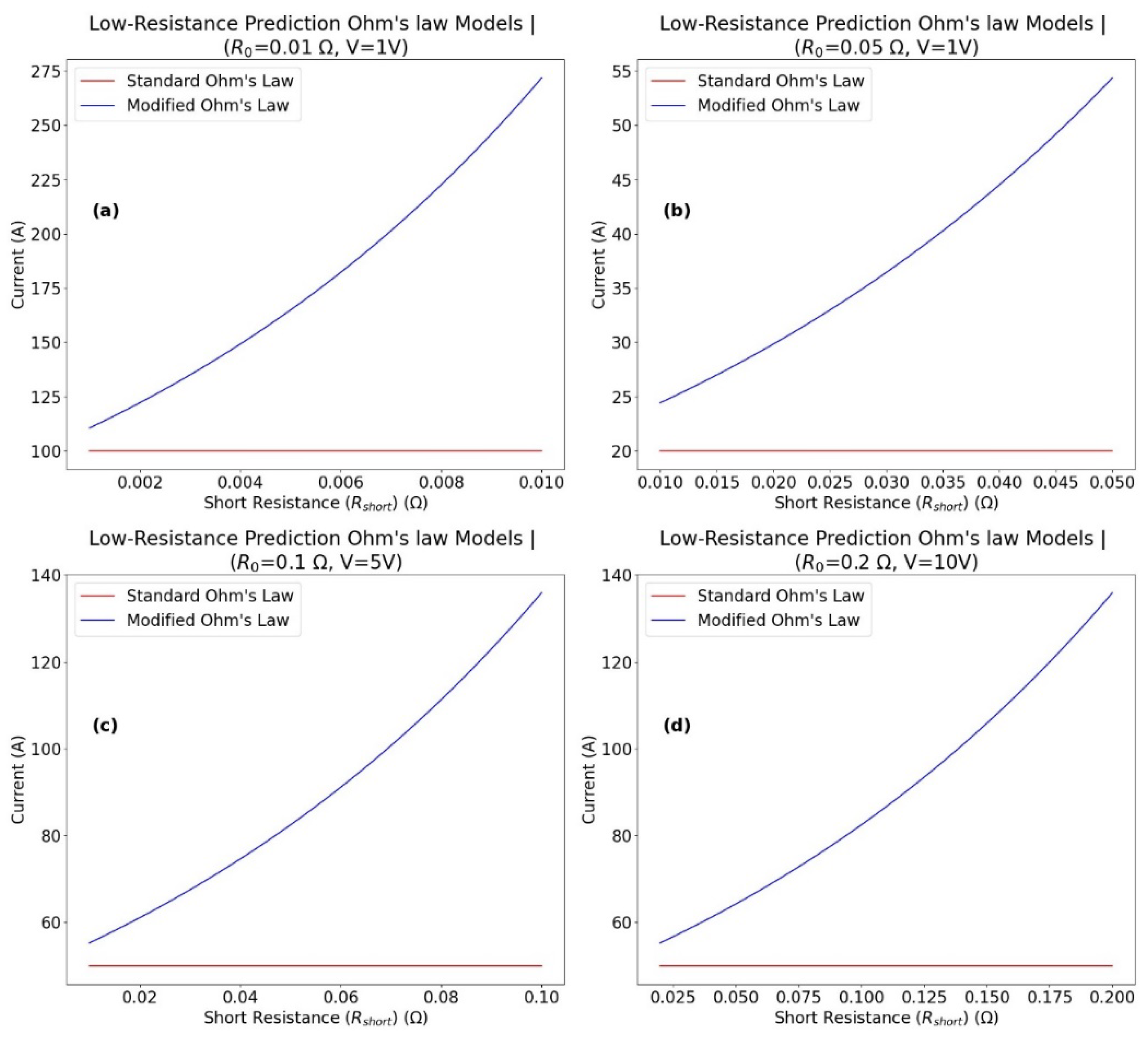
Figure 2.
High-Current Prediction on Ohm’s Law Models for , and . ((a) , , ; (b) , , ; (c) , , ; (d) , , . These plots compare the Standard Ohm’s Law (red) and Modified Ohm’s Law (blue) predictions, highlighting the modified model's ability to maintain accurate current predictions under high-current conditions. In all panels (a)-(d)), the resistance ranged uniformly between and ).
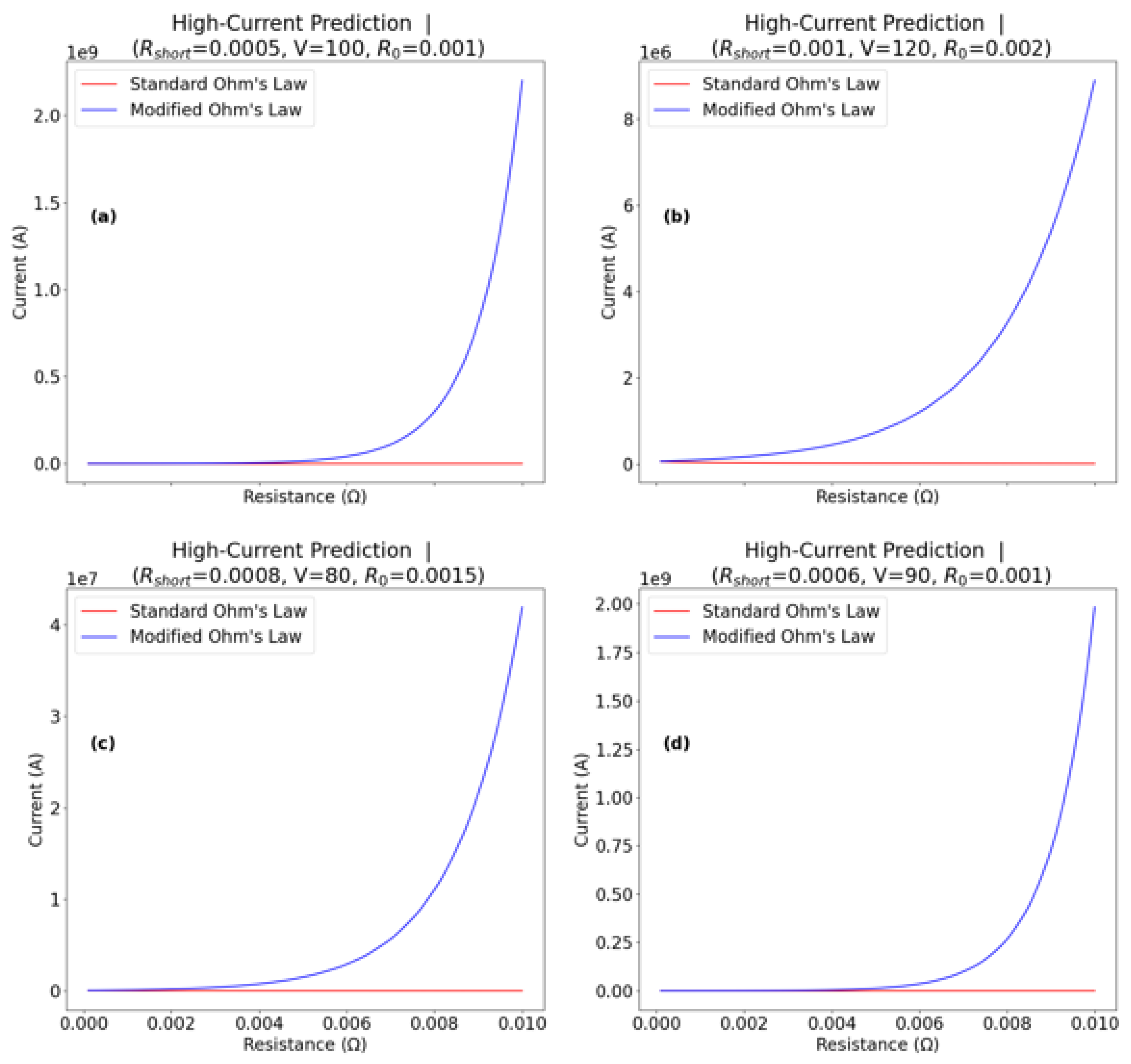
Figure 3.
High-Current Prediction Results for , and . ((a) , , ; (b) , , ; (c) , , ; (d) , , varying . These plots compare the Standard Ohm’s Law (red) and Modified Ohm’s Law (blue) predictions, highlighting the modified model's ability to maintain accurate current predictions under various high-current conditions In all panels (a)-(d)), the resistance ranged uniformly between and ).
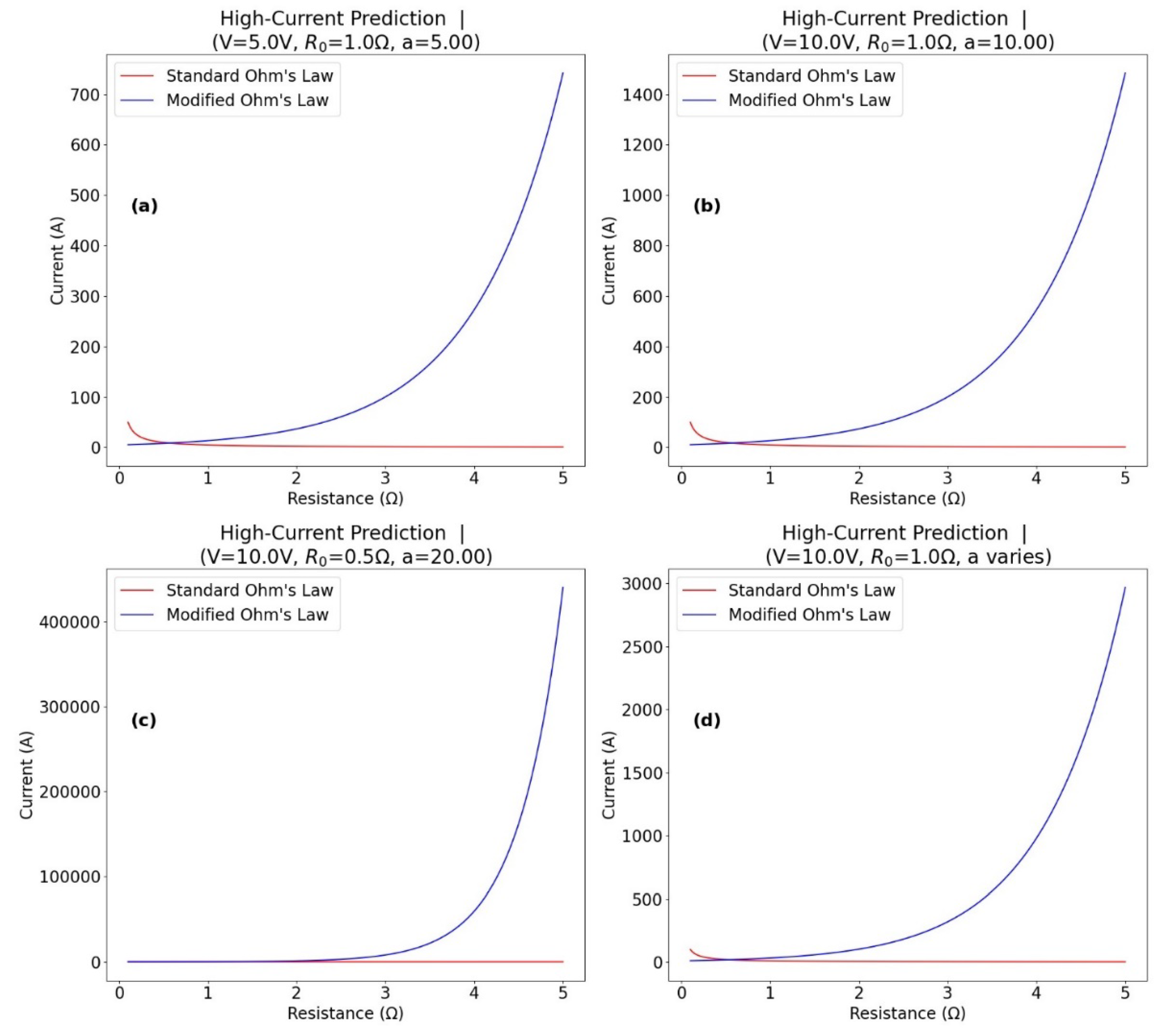
Figure 4.
High-Frequency Circuit Analysis Results. ((a-d) at , (e-h) at , (i-l) at . These plots compare the Standard Ohm’s Law (red) and Modified Ohm’s Law (blue) predictions, demonstrating the Modified Ohm’s Law model’s ability to accurately predict current across various high-frequency conditions. Each panel details a different combination of , , and , illustrating the versatility and accuracy of the Modified Ohm’s Law in advanced circuit design and analysis. In all panels (a)-(l)), the resistance ranged uniformly between and ).
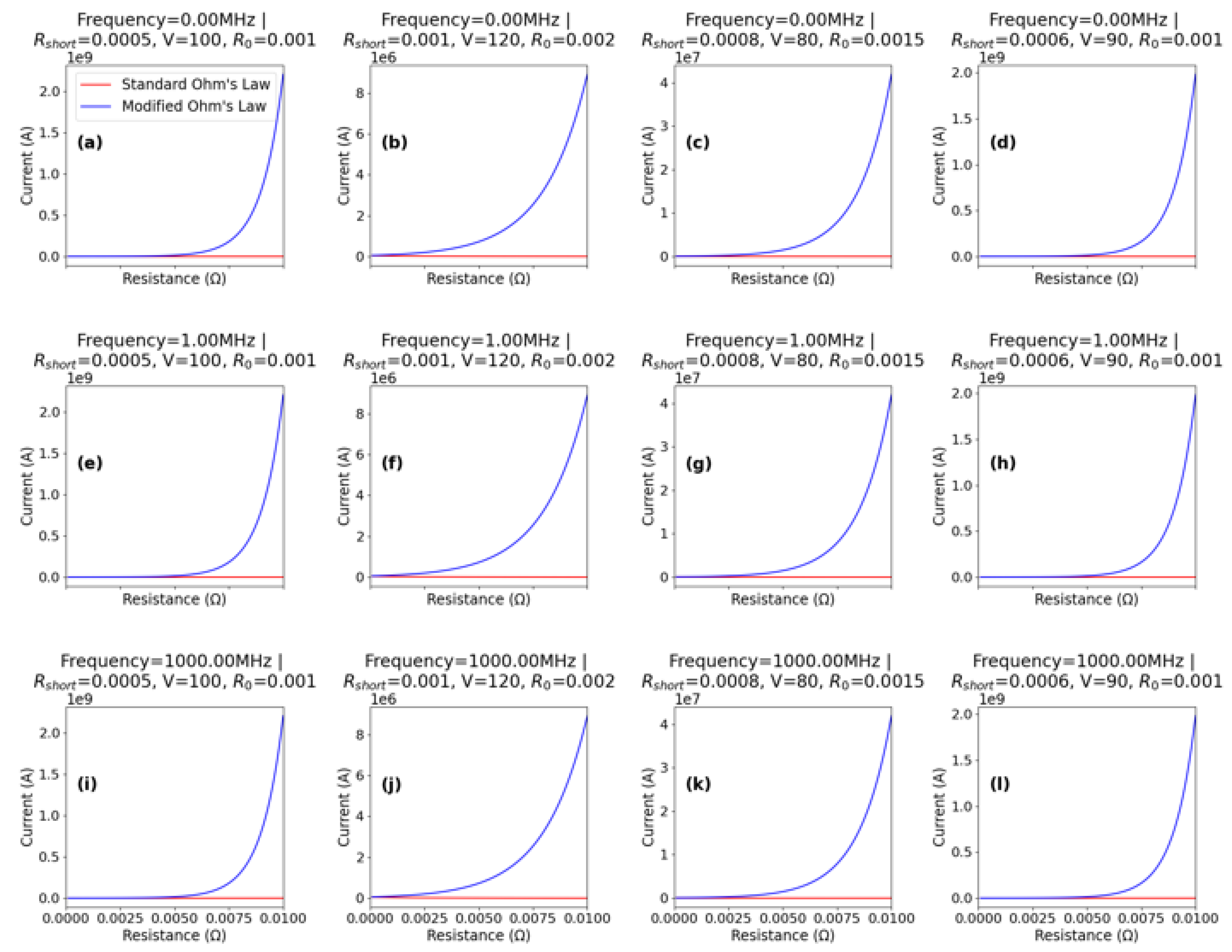
Figure 5.
Comparative Current Predictions Using Standard and Modified Ohm’s Law. ((a) Semiconductor, (b) Thermistor, (c) Varistor, (d) Non-uniform Resistivity Material. Each plot compares the Standard Ohm’s Law (red) with the Modified Ohm’s Law (blue), highlighting the latter's ability to capture the non-linear behavior of these devices across different resistance ranges and voltages).
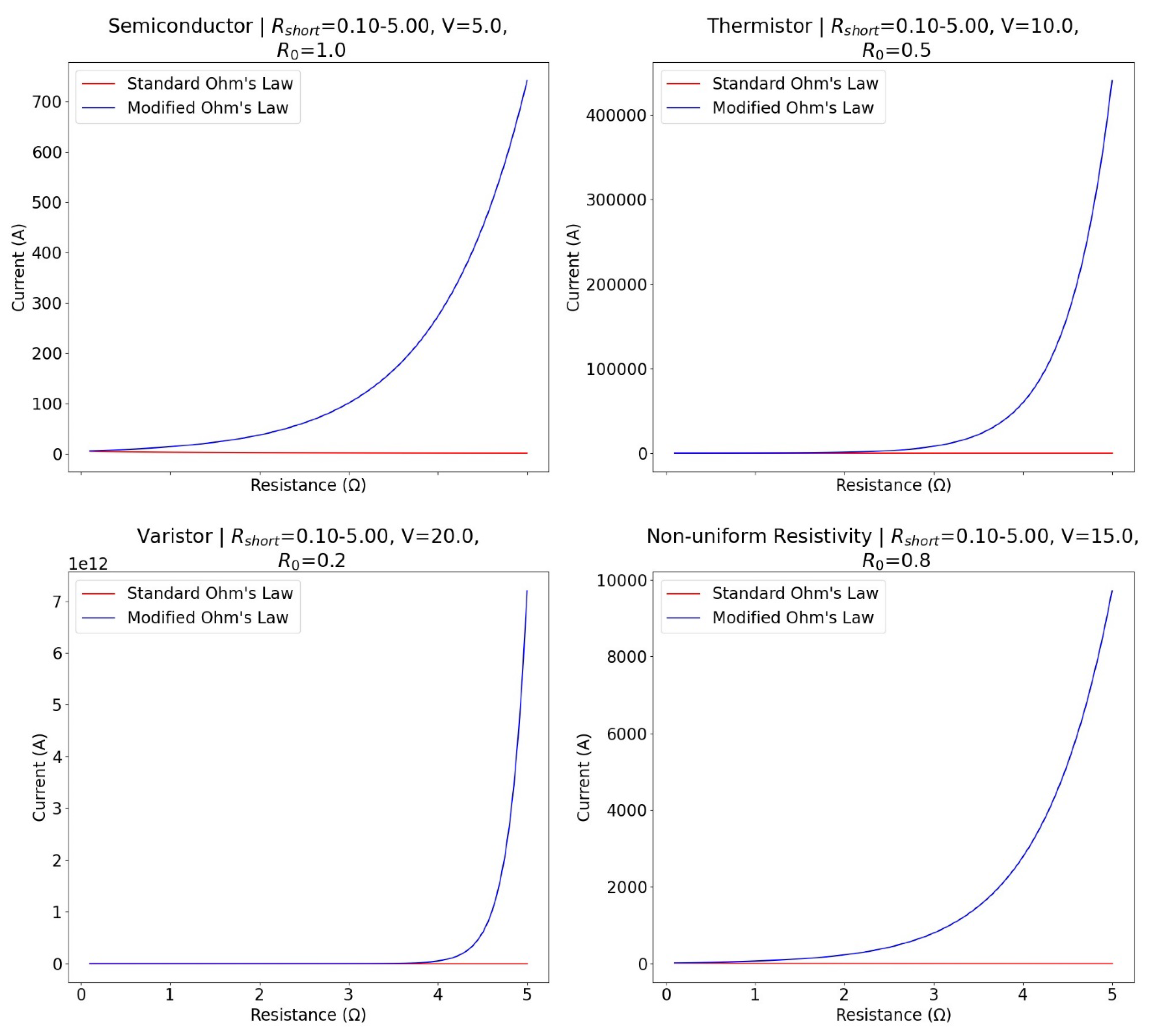
Figure 6.
Comparative Current Predictions Using Standard Ohm’s Law and Modified Ohm’s Law Variants. ((a) WiFi Router, (b) Cellular Base Station, (c) Satellite Communication, (d) Radar System. Each plot compares the Standard Ohm’s Law (red) with the Modified Ohm’s Law (blue), highlighting the latter's ability to capture the non-linear behavior of these systems across different resistance ranges and voltages).
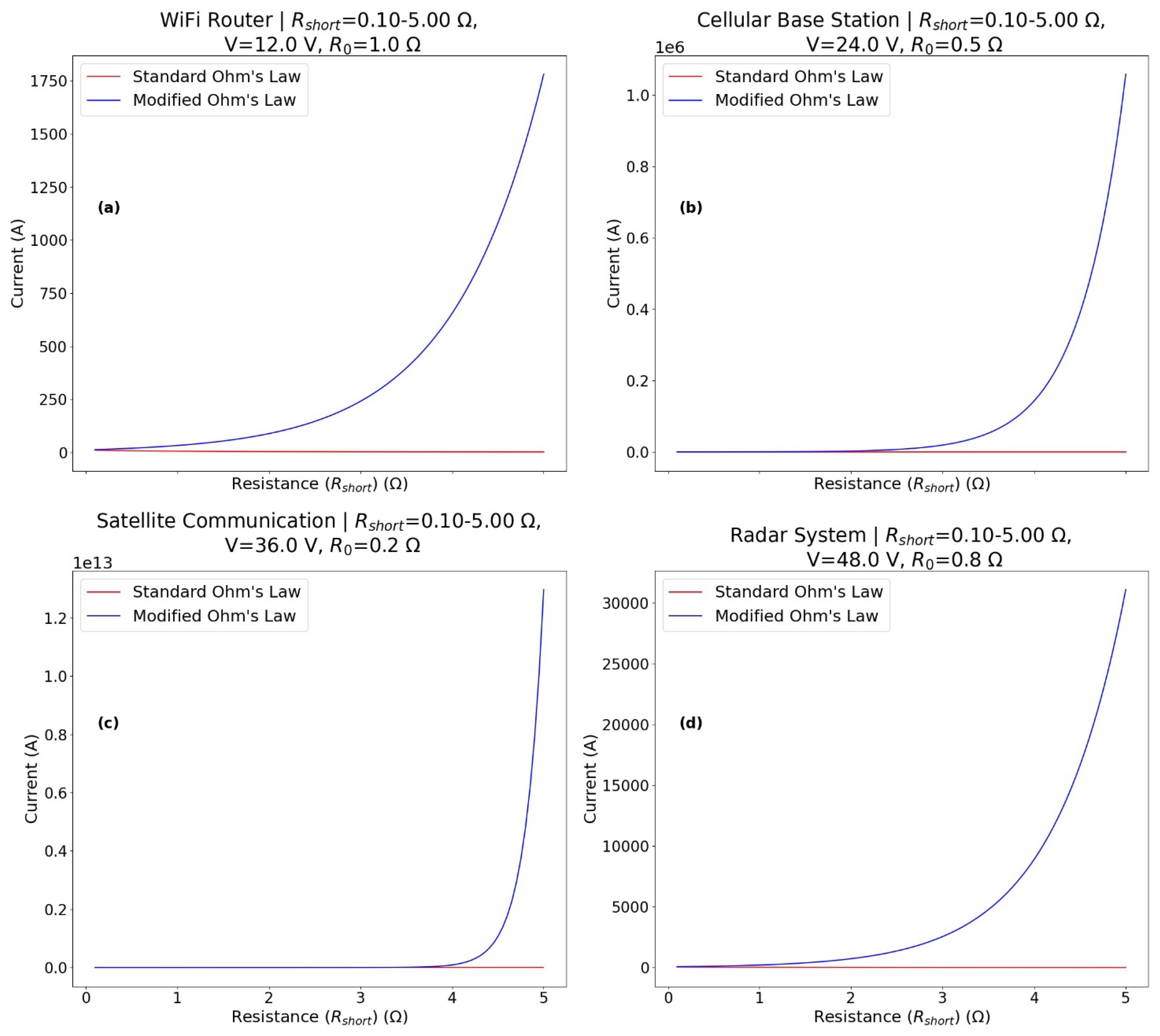
Table 1.
Simulation Algorithm Framework.
| Parameter Initialization |
|
| Current Calculation |
|
| Comparative Analysis |
|
Disclaimer/Publisher’s Note: The statements, opinions and data contained in all publications are solely those of the individual author(s) and contributor(s) and not of MDPI and/or the editor(s). MDPI and/or the editor(s) disclaim responsibility for any injury to people or property resulting from any ideas, methods, instructions or products referred to in the content. |
© 2024 by the authors. Licensee MDPI, Basel, Switzerland. This article is an open access article distributed under the terms and conditions of the Creative Commons Attribution (CC BY) license (http://creativecommons.org/licenses/by/4.0/).
Copyright: This open access article is published under a Creative Commons CC BY 4.0 license, which permit the free download, distribution, and reuse, provided that the author and preprint are cited in any reuse.


