
Submitted:
14 August 2024
Posted:
15 August 2024
You are already at the latest version
Abstract
In this study, we evaluate the nonlinear dynamics of convection flow using the thermodynamic variational principle, focusing on scenarios where multiple external forces, such as a thermal gradient and rotational field, are applied to a shallow annular pool. We observed that with the increase in the thermal gradient, the flow changed from an axial flow to a rotational oscillatory flow with the wave amplitudes aligned. Further increasing the temperature difference led to a rotational oscillatory flow characterized by alternating wave generation and annihilation. Our analysis of the flow, considering heat fluxes orthogonal to the thermal gradient, allowed us to describe the flow state as a phase at equilibrium. The state transition of the flow was accompanied by a discontinuous jump in the heat flux, which occurred at the intersection of the entropy production curves.
Keywords:
nonlinear dynamics
; thermal convection
; entropy production
; variational principle
; rotational field
1. Introduction
Understanding the phenomena of transitions in the spatiotemporal structure of spontaneous convection under an applied external field is crucial in fundamental physics and industries. In fundamental physics, it relates to key areas such as nonlinear dynamics and nonequilibrium thermodynamics related to fluid instabilities [1,2,3,4]. In industries, these transitions are crucial for manufacturing process using transport phenomena [5,6,7,8,9]. Rayleigh–Bénard convection—a classic example of thermal convection—has been extensively studied both theoretically and experimentally for many years [10,11,12,13,14,15,16,17]. Chandrasekhar stated that the symmetry breaking of Bénard convection is sustained by the competition between the viscosity-induced dissipation of kinetic energy and the internal energy released by buoyancy [18]. He obtained stable conditions for convection generation. Hohenberg and Swift analyzed the complex behavior of Bénard convection under temporally modulated temperature differences using the Lorenz model [19]. They obtained a bifurcation diagram that illustrates the transition process not only from conductive heat transfer to Bénard convection but also from a hexagonal pattern to a roll pattern.
Recently, attempts have been made to theoretically analyze the evolution of nonequilibrium states in systems where various irreversible processes are coupled, using the variational principle of maximum entropy production (MEPP) [20,21,22,23,24]. The MEPP shows that nonequilibrium states evolve into more complex states that generate higher entropy. Here, "complex" refers to the interference between two or more irreversible processes [25]. When two fluids with different viscosities are displaced in a Hele–Shaw cell, the interface becomes destabilized, transitioning from a stable diffusion interface to a finger-like interface due to the Saffman–Taylor instability as the viscosity ratio increases [26]. With a further increase in the viscosity ratio, the flow becomes more complex owing to the splitting of the viscous fingers [27,28]. The flow at the growing interface evolves such that entropy production is maximized [29]. The transition of Bénard convection from a hexagonal to a rolled pattern owing to temperature modulation transitions to a pattern with higher entropy production [30]. The bistability of the hexagonal and rolled patterns arises because, while the rolled pattern exhibits higher heat flux, the hexagonal pattern still produces higher entropy.
In addition to predicting the state transitions, the variational principle can be used to derive the governing equations for complex transport phenomena. Doi et al. derived the time evolution equations for the contact line and droplet shape in the dynamics of an evaporating droplet, driven by the Marangoni effect [31]. They also derived time-evolution equations for deposition patterns, such as coffee rings and mountain shapes, during the drying process of the liquid film [32]. Thus, the MEPP has significantly advanced our understanding of various nonequilibrium phenomena. However, it remains unknown whether MEPP can be applied to complex transport phenomena involving multiple external forces. In this study, we quantitatively analyzed the state transitions of thermal convection in a system under a rotational field using the MEPP.
2. Equations of Motion and Numerical Details
Figure 1 shows the schematic of an annular pool with an applied temperature difference. A shallow annular pool with an inner wall of 15 mm , an outer wall of 50 mm , and a depth of 3 mm was filled with a silicon melt. The inner wall is fixed at the melting point of silicon, , and the outer wall is set at a higher temperature than the inner wall, . The upper liquid surface is a free interface, where Marangoni convection is used. No-slip conditions were imposed on the fluid velocities on all solid walls (inner and outer walls and bottom). The numerical analysis was performed in OpenFOAM using the PISO method, with discretization achieved through the finite volume method. The grid numbers are 81, 180, and 21 in the radial, circumferential, and vertical directions, respectively. This grid configuration, based on the conditions established by Li et al.,[33] sufficiently captures HTW in low-Pr fluids.
Assuming that the silicon melt behaves as an incompressible Newtonian fluid and the Boussinesq approximation is applicable, the continuity, Navier–Stokes, and energy equations can be expressed as
where andare the velocity, density, kinematic viscosity, and thermal diffusivity of the fluid, respectively. Additionally, is pressure, is temperature, and is time. We assume that if a subscript appears more than once in the same term in the equation, summation over the repeated subscripts is implied. In this thermally driven system, spontaneous convection, resulting from the density difference, and Marangoni convection, resulting from the surface tension difference, coexist. However, the former can be neglected because the density changes owing to temperature differences are small. Therefore, it is unnecessary to consider the buoyancy term in Eq (2) [34]. Initially, there was no convection in the annular pool, and the fluid temperature was set uniformly at 1683 K, which is the melting point of silicon. Convection is induced by the Marangoni effect owing to the presence of a thermal gradient on the free surface, according to the following equation:
where and are the viscosity and the surface tension coefficient of the fluid, respectively. The fluid properties and computational parameters used in the numerical calculations are listed in Table 1.
Increasing the temperature difference between the inner and outer walls results in the transition of the flow state in the system from an axially symmetric flow (ASF) to a rotating oscillatory flow called hydrothermal waves (HTW) [35]. The former is a radially symmetric flow, while the latter causes convection in the circumferential direction. The transition point of the flow state in the system is at approximately . Figure 1b shows a typical ASF and HTW displayed in terms of surface temperature fluctuation . For ASF, the distribution is almost uniform, showing no significant temperature difference. In contrast, for HTW, a radial region with alternating hot and cold regions appears and rotates in the circumferential direction.
In a fluid undergoing an irreversible process, the rate of entropy production, , can expressed via the entropy produced per unit volume (s) and the conserved quantity () using the following equation [36].
Subscript k represents the conserved quantity. Energy is transported by heat conduction, momentum is transported by fluid movement, and matter is transported by mass transfer. Entropy is produced in the fluid because of the irreversible transport of conserved quantities through the driving force. Thus, the entropy production can be expressed as:
Here, represents the local driving force, and represents the transport of conserved quantities in response to the driving force. In thermal convection, two irreversible processes interact: the transport of energy via heat conduction and the transport of momentum via fluid movement. Because the entropy production of the latter is significantly smaller than that of the former, only the entropy production by the heat flux is considered here [34]. Therefore, subscript k is omitted. Experiments have demonstrated that even with complex flow patterns, such as those of a Bénard cell, the heat flux is linear with respect to the driving force [37,38]. This leads to the following equation:
where is the thermal conductivity of the fluid. Entropy production is a scalar quantity that represents the amount of heat produced per unit volume due to the thermal gradient in each direction. However, because certain components are highly related to the symmetry with respect to the driving force that keeps the system nonequilibrium, we will denote entropy production separately for each gradient in this study.
As the system is far from equilibrium, both and are time-dependent and spatially distributed. To characterize the nonequilibrium state of the system through space- and time-dependent thermodynamic quantities, local thermodynamic quantities at point A = (30 mm, 0 mm, 3 mm) were calculated by time averaging.
where = 200 s and = 300 s. Additionally, represents the time interval . The entropy production was calculated as the product of and , as shown in Equation (9). In addition to the thermal gradient, a counterclockwise rotational field with was applied to the annular pool to assess changes in the flow state and to measure heat flux and entropy production.
3. Results and Discussion
Figure 2 shows changes in temperature at point A on the fluid surface for different rotational velocities at . In the absence of a rotating field, HTW occurs with a fluctuation range of approximately 0.7 K, with a period of approximately 7 s. For , the HTW is a combination of long-term oscillations, with a period of approximately 90 s, and short-term oscillations, with a period of approximately 2 s. The temperature fluctuation of the long-term oscillation was comparable to that without rotation, whereas that of the short-term oscillation was approximately one-third that of the long-term oscillation. At , the long-term oscillation disappeared, and the temperature fluctuation resulted in a constant-amplitude HTW with a period of approximately 1.5 s. For , the temperature fluctuation disappeared, and the ASF appeared. Theoretical studies have shown that the addition of a rotating field stabilizes thermal convection [18].
Figure 3 shows the entropy production in each direction calculated using Equations (10) and (11) as a function of the thermodynamic force at . As increases, increases parabolically. The largest entropy production, , occurs in the x-direction due to heat flux, as it aligns with the thermal gradient on the inner and outer walls, which serves as the driving force. This is followed by and . If the flow effect is ignored and entropy production is considered to solely result from heat conduction according to Fourier’s law, it can theoretically be expressed as [34]. When the theoretical values were plotted using the average temperature , the acquired data closely matched the theoretical predictions. Even when the flow state changed from ASF to HTW, the entropy production data exhibited the same curve. This result accurately reflects the increase in entropy production owing to local driving forces but also indicates that changes in state cannot be distinguished by expressing entropy production solely as a function of thermodynamic forces.
Determining function to changes in nonequilibrium states is a critical issue. Previous experimental and computational examples have shown that using a function of the global driving force that maintains the nonequilibrium state of the system is effective [39,40]. The emergence of new flow states owing to symmetry breaking in response to the global driving force is often observed in various transport phenomena, such as Bénard convection, Marangoni convection, and the Saffman–Taylor instability [29,30,34,41]. A common feature of this phenomenon is the production of excess entropy in the direction orthogonal to the global driving force. This excess entropy is produced by thermodynamic flux in the direction of symmetry breaking. This thermodynamic flux is referred to as the emergent flux. When the emergent flux is considered as a function of the global driving force, the entropy production similarly becomes a function of the global driving force.
where , and are phenomenological coefficients. In particular, is significant as it is related to the free energy required to transition from one state to another and is also related to the degree of coherence of two or more irreversible processes [39,42]. Because the phenomenological coefficients are different for the different states of the system, the states of the system can be described by different lines. Using this relationship between the emergent flux and the global driving force, we can identify the state of the system. The entropy production for each nonequilibrium state can then be obtained using Equation (13). According to the MEPP, the thermodynamic flux changes such that the system transitions to a state with a higher entropy production. For the Bénard convection, the global driving force is the thermal gradient provided above and below the vessel[30,37]. As the driving force increased, the thermodynamic flux changed discontinuously with each transition from conduction to convective heat transfer and from hexagonal to roll patterns. Discontinuity represents the transition point of the nonequilibrium state, which is represented by the intersection of the entropy production curves. The MEPP, using the relationship between the emergent flux and global driving force, was used to quantitatively describe complex transitions in thermal convection under a rotating field. Additionally, it was used to predict the transition point.
In this thermally driven system, the thermal gradient provided on the inner and outer walls is the driving force that changes the state of the thermal convection inside. We express the thermal gradient in terms of the dimensions of the thermodynamic force, referring to it as the global driving force .
The heat fluxes in the x- and y-directions at each rotational speed are shown in Figure 4. The lower and upper abscissae represent the global driving force and the corresponding temperature difference , respectively. The numerical values of are similar to those of , except for an order of magnitude. increased linearly with respect to the global driving force regardless of the rotational speed. If the flow effects are disregarded and only heat conduction according to Fourier’s law is considered, the heat flux is theoretically expressed as [34]. The heat flux in the x-direction was almost consistent with the theoretical equation and was independent of the rotational speed. As the direction of the global thrust was radial, it agreed with the thermal gradient in the x-direction at the measurement point. Marangoni convection occurred in the x-direction at the free surface; however, the effect of the flow on the heat flux in the x-direction was negligible because the conduction heat transfer was more dominant. The heat flux in the y-direction, where the symmetry was broken by the global driving force, exhibited a nontrivial trend. In the absence of a rotational field, can be described by different straight lines for ASF and HTW using Equation (12). For ASF, passes through the origin and , indicating a complete absence of interfering nature with other irreversible processes. For HTW, exhibits a finite value, indicating the degree of interference from other irreversible processes. In the presence of a rotational field, was on the same line as ASF, independent of the rotational speed; however, the value of the global driving force required to generate HTW increased significantly with increasing rotational speed. This indicates that the centrifugal force generated by the rotational field suppresses HTW generation. As the global driving force further increased, a discontinuous change in the heat flux was observed, and the slope of the straight line became even larger. This implies the existence of a different convection pattern.
The emergent heat flux results suggest the presence of a new HTW flow pattern. Figure 5 illustrates the surface temperature fluctuations for (top panels) and (bottom panels) at . For , time progresses from the left to the right panels at an interval of 0.6 s. Waves consisting of eight pairs of high- and low-temperature regions are generated from the inner wall, expanding radially while rotating counterclockwise. When the tip of the growing wave reaches half of the annular pool, the wave detaches from the inner wall and diffuses toward the outer wall. New waves reappear from the inner wall. This results in heat waves propagating in the circumferential direction, with waves being repeatedly generated and annihilated. A normal rotating oscillating flow with constant width and length that rotates in one direction is represented by HTW. On the other hand, a rotating oscillating flow that repeatedly generates and annihilates waves is represented as HTW. In the presence of a rotating field, the heat flux region represented by the straight line with the steepest slope in Figure 4a corresponds to the region where HTW is observed.
The transitions from ASF to HTW and from HTW to HTW are discussed using MEPP. Figure 6 shows the emergent heat flux and the corresponding entropy production at . To obtain the entropy production curve, we first determined the differential coefficient at each point of the heat flux. The heat flux was divided into three regions based on the differential coefficient values. In the regions divided by differential coefficients, the heat flux was fitted using Equation (12), providing three straight lines with different values of L’ and Θ. The entropy production in each region was fitted using Equation (13) with Θ in common, resulting in three entropy curves. The fitting parameters for each region are listed in Table 2.
The entropy production curves of ASF and HTW intersect at while those of HTW to HTWintersect at . This is nearly consistent with the point where the emergent heat flux changes discontinuously. Additionally, at , the transition point was accurately predicted using MEPP. Three key observations can be observed from these results. First, MEPP effectively predicts the transition point of the state even in a nonequilibrium system with multiple external forces, including the addition of thermal gradients and rotational fields. Second, the relationship between the emergent heat flux and the global driving force leads to the discovery of new flow states. Third, the relationship between the emergent heat flux and global driving force allows the specification of nonequilibrium states to be specified as if they were a phase of an equilibrium system.
For example, in equilibrium, if the state of water can be categorized into solid, liquid, and vapor phases, each state can be represented by a distinct function, with the chemical potential expressed as a function of temperature (Figure 7a). The entropy per mole can be obtained from the slope as: . Because , the chemical potential decreased as the temperature increased. The entropy increased in the order , leading to steeper gradients in the same order. For , extrapolation of for each phase shows that the solid phase is the most stable because it has the lowest μ. For , the liquid phase is stable because it has the lowest the μ, while for , the gas phase is stable because it has the lowest μ. The phase transition point can be observed at the intersection of of each phase. These results are logical consequences of the principle of maximum entropy.
In nonequilibrium, if the emergent flux is expressed as a function of the global driving force , each state can be described by a different function, allowing the nonequilibrium state to be defined as a phase, analogous to how chemical potential defines phases in equilibrium systems. As increases, increases, which can be accompanied by a discontinuity change at the transition point and an increase in slope. Therefore, the system evolves into a state with higher entropy production. Therefore, to achieve a higher entropy production rate, the system interferes with other irreversible processes and discontinuously changes into a state with higher flux. This leads to a state transition from ASF to HTW and further to HTW.
4. Conclusion
This study quantitatively analyzed the state transitions of the flow in a thermally convective system under an applied thermal gradient and rotational field using MEPP. Using a heat flux orthogonal to the applied thermal gradient, the three states of thermal convection, ASF, HTW, and HTW, were described by distinct straight lines. The transition points between states are identified by the intersections of the entropy production curves for each state. This suggests that in nonequilibrium, state transitions are driven by changes in flux, as these changes lead to faster entropy production. The MEPP may have a certain universality, because it is found not only in thermal convection phenomena but also in various transport phenomena such as Marangoni convection and Saffman–Taylor instability. Because of the analogy with equilibrium thermodynamics in terms of phase description and stability, a theorem similar to the equilibrium system may be derived for the nonequilibrium system. Verification of the theorem will lead to further development of the MEPP.
Author Contributions
Conceptualization, T.B.; methodology, R.F. and K.S.; validation, R.F. and K.S.; formal analysis, T.B.; investigation, T.B.; data curation, R.F. and K.S.; writing—original draft preparation, T.B.; writing—review and editing, T.B., R.F. and K.S.; visualization, T.B.; project administration, T.B.; All authors have read and agreed to the published version of the manuscript.
Funding
This research was funded by JSPS KAKENHI, grant number 24K07304.
Conflicts of Interest
The authors declare no conflicts of interest.
References
- Onsager, L. Reciprocal Relations in Irreversible Processes. I. Phys. Rev. 1931, 37, 405–426. [CrossRef]
- Onsager, L. Reciprocal Relations in Irreversible Processes. II. Phys. Rev. 1931, 38, 2265–2279. [CrossRef]
- Prigogine, I. Introduction to Thermodynamics of Irreversible Processes; Charles C Thomas: Illinois, 1956;
- Hohenberg, P.; Halperin, B. Theory of dynamic critical phenomena. Rev. Mod. Phys. 1977, 49, 435–479. [CrossRef]
- Schwabe, D.; Scharmann, A.; Preisser, F.; Oeder, R.; Liebig-universitdt, I.P.I.D.J.; Germany, W. Experiments on surface tension driven flow in floating zone melting. J. Cryst. Growth 1978, 43, 305–312.
- Hu, H.; Larson, R.G. Marangoni effect reverses coffee-ring depositions. J. Phys. Chem. B 2006, 110, 7090–7094. [CrossRef]
- Deegan, R.D.; Bakajin, O.; Dupont, T.F.; Huber, G.; Nagel, S.R.; Witten, T.A. Capillary flow as the cause of ring stains from dried liquid drops. Nature 1997, 389, 827–829. [CrossRef]
- Bejan, A. A Study of Entropy Generation in Fundamental Convective Heat Transfer. J. Heat Transfer 1979, 101, 718–725. [CrossRef]
- Bejan Adrian Bejan - Advanced Engineering Thermodynamics (2006, Wiley) - libgen.lc 2006.
- Pearson, J.R.A. On convection cells induced by surface tension. J. Fluid Mech. 1958, 4, 489–500. [CrossRef]
- Nield, D.A. Surface tension and buoyancy effects in cellular convection. J. Fluid Mech. 1964, 19, 341–352. [CrossRef]
- GROSSMANN, S.; LOHSE, D. Scaling in thermal convection: a unifying theory. J. Fluid Mech. 2000, 407, 27–56. [CrossRef]
- Farmer, J.D.; Sidorowich, J.J. Predicting chaotic time series. Phys. Rev. Lett. 1987, 59, 845–848. [CrossRef]
- Busse, B.F.H. The stability of finite amplitude cellular convection and its relation to an extremum principle. J. Fluid Mech. 1967, 30, 625–649.
- Malkus, W.V.R.; Veronis, G. Finite amplitude cellular convection. J. Fluid Mech. 1958, 4, 225–260. [CrossRef]
- Bodenschatz, E.; Pesch, W.; Ahlers, G. R ECENT D EVELOPMENTS IN R AYLEIGH -B E. 2000, 709–778.
- Chatterjee, A.; Yadati, Y.; Mears, N.; Iannacchione, G. Coexisting Ordered States, Local Equilibrium-like Domains, and Broken Ergodicity in a Non-turbulent Rayleigh-Bénard Convection at Steady-state. Sci. Rep. 2019, 9, 10615. [CrossRef]
- Chandrasekhar, S. Hydrodynamic and Hydromagnetic Stability; Oxford University Press: Oxford, 1961;
- Hohenberg, P.C.; Swift, J.B. Hexagons and rolls in periodically modulated Rayleigh-Bénard convection. Phys. Rev. A 1987, 35, 3855–3873. [CrossRef]
- Doi, M. Onsager’s variational principle in soft matter. J. Phys. Condens. Matter 2011, 23, 284118. [CrossRef]
- Martyushev, L.M.; Seleznev, V.D. Maximum entropy production principle in physics, chemistry and biology. Phys. Rep. 2006, 426, 1–45. [CrossRef]
- Martyushev, L.M. Мaximum Entropy Production Principle: History and Current Status. Uspekhi Fiz. Nauk 2021, 191, 586–613. [CrossRef]
- Endres, R.G. Entropy production selects nonequilibrium states in multistable systems. Sci. Rep. 2017, 7, 1–13. [CrossRef]
- Lucia, U.; Grisolia, G.; Ponzetto, A.; Silvagno, F. An engineering thermodynamic approach to select the electromagnetic wave effective on cell growth. J. Theor. Biol. 2017, 429, 181–189. [CrossRef]
- Ziegler, H. An introduction to thermomechanics; North Holland, Amsterdam, 1977; ISBN 3804204422.
- Saffman, P.G.; Taylor, G. The Penetration of a Fluid into a Porous Medium or Hele-Shaw Cell Containing a More Viscous Liquid. Proc. R. Soc. A 1958, 245, 312–329. [CrossRef]
- Martyushev, L.M.; Birzina, A.I.; Konovalov, M.S.; Sergeev, A.P. Experimental investigation of the onset of instability in a radial Hele-Shaw cell. Phys. Rev. E - Stat. Nonlinear, Soft Matter Phys. 2009, 80, 1–9. [CrossRef]
- Martyushev, L.M.; Bando, R.D.; Chervontseva, E.A. Instability of the fluid interface at arbitrary perturbation amplitudes. Displacement in the Hele–Shaw cell. Phys. A Stat. Mech. its Appl. 2021, 562, 125391. [CrossRef]
- Ban, T.; Ishii, H.; Onizuka, A.; Chatterjee, A.; Suzuki, R.X.; Nagatsu, Y.; Mishra, M. Momentum transport of morphological instability in fluid displacement with changes in viscosity. Phys. Chem. Chem. Phys. 2024, 26, 5633–5639. [CrossRef]
- Ban, T. Thermodynamic Analysis of Bistability in Rayleigh–Bénard Convection. Entropy 2020, 22, 800. [CrossRef]
- Man, X.; Doi, M. Vapor-Induced Motion of Liquid Droplets on an Inert Substrate. Phys. Rev. Lett. 2017, 119, 1–5. [CrossRef]
- Man, X.; Doi, M. Ring to Mountain Transition in Deposition Pattern of Drying Droplets. Phys. Rev. Lett. 2016, 116, 1–5. [CrossRef]
- Peng, L.; Li, Y.R.; Shi, W.Y.; Imaishi, N. Three-dimensional thermocapillary-buoyancy flow of silicone oil in a differentially heated annular pool. Int. J. Heat Mass Transf. 2007, 50, 872–880. [CrossRef]
- Ban, T.; Shigeta, K. Thermodynamic analysis of thermal convection based on entropy production. Sci. Rep. 2019, 9, 10368. [CrossRef]
- Schwabe, D.; Zebib, A.; Sim, B.C. Oscillatory thermocapillary convection in open cylindrical annuli. Part 1. Experiments under microgravity. J. Fluid Mech. 2003, 491, 239–258. [CrossRef]
- De Groot, S.R.; Mazur, P. Non-Equilibrium Thermodynamics; Dover: New York, 1984; ISBN 0486647412.
- Meyer, C.W.; Cannell, D.S.; Ahlers, G.; Swift, J.B.; Hohenberg, P.C. Pattern Competition in Temporally Modulated Rayleigh-Bénard Convection. Phys. Rev. Lett. 1988, 61, 947–950. [CrossRef]
- Chatterjee, A.; Ban, T.; Iannacchione, G. Evidence of local equilibrium in a non-turbulent Rayleigh–Bénard convection at steady-state. Phys. A Stat. Mech. its Appl. 2022, 593, 126985. [CrossRef]
- Hill, A. Entropy production as the selection rule between different growth morphologies. Nature 1990, 348, 426–428. [CrossRef]
- Martyushev, L.M. Some interesting consequences of the maximum entropy production principle. J. Exp. Theor. Phys. 2007, 104, 651–654. [CrossRef]
- Ban, T.; Hatada, Y.; Takahashi, K. Spontaneous motion of a droplet evolved by resonant oscillation of a vortex pair. Phys. Rev. E - Stat. Nonlinear, Soft Matter Phys. 2009, 79, 1–12. [CrossRef]
- Nabika, H.; Tsukada, K.; Itatani, M.; Ban, T. Tunability of Self-Organized Structures Based on Thermodynamic Flux. 2022. [CrossRef]
Figure 1.
(a) Schematic of an annular pool. (b) Color map of surface temperature fluctuation, , for typical axially symmetric flow (left) and hydrothermal waves (right).
Figure 1.
(a) Schematic of an annular pool. (b) Color map of surface temperature fluctuation, , for typical axially symmetric flow (left) and hydrothermal waves (right).

Figure 2.
Evolution of surface temperature at different rotational speeds.
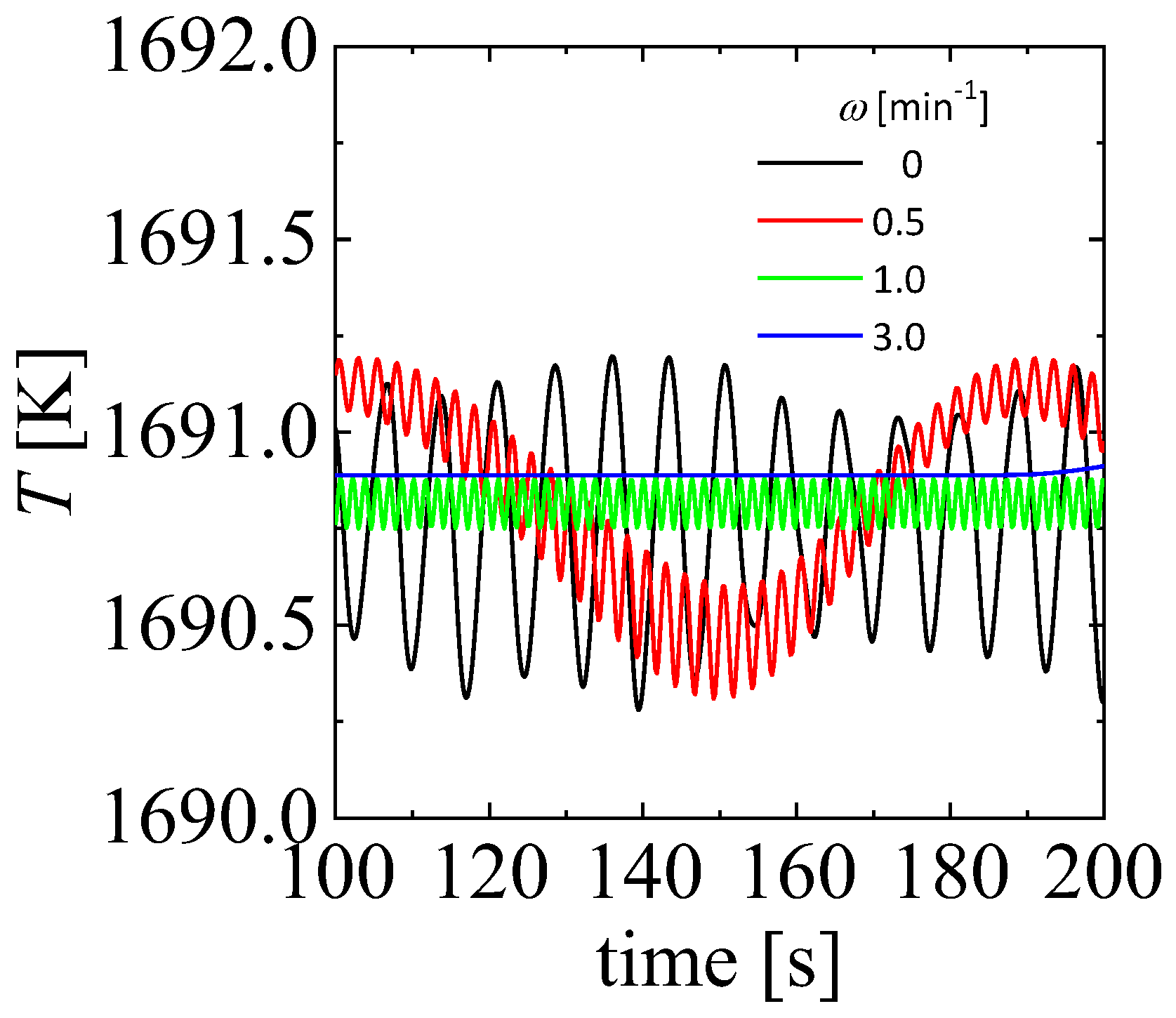
Figure 3.
Relationship between the entropy production and the thermodynamic force generated by the heat flux in each direction at .
Figure 3.
Relationship between the entropy production and the thermodynamic force generated by the heat flux in each direction at .
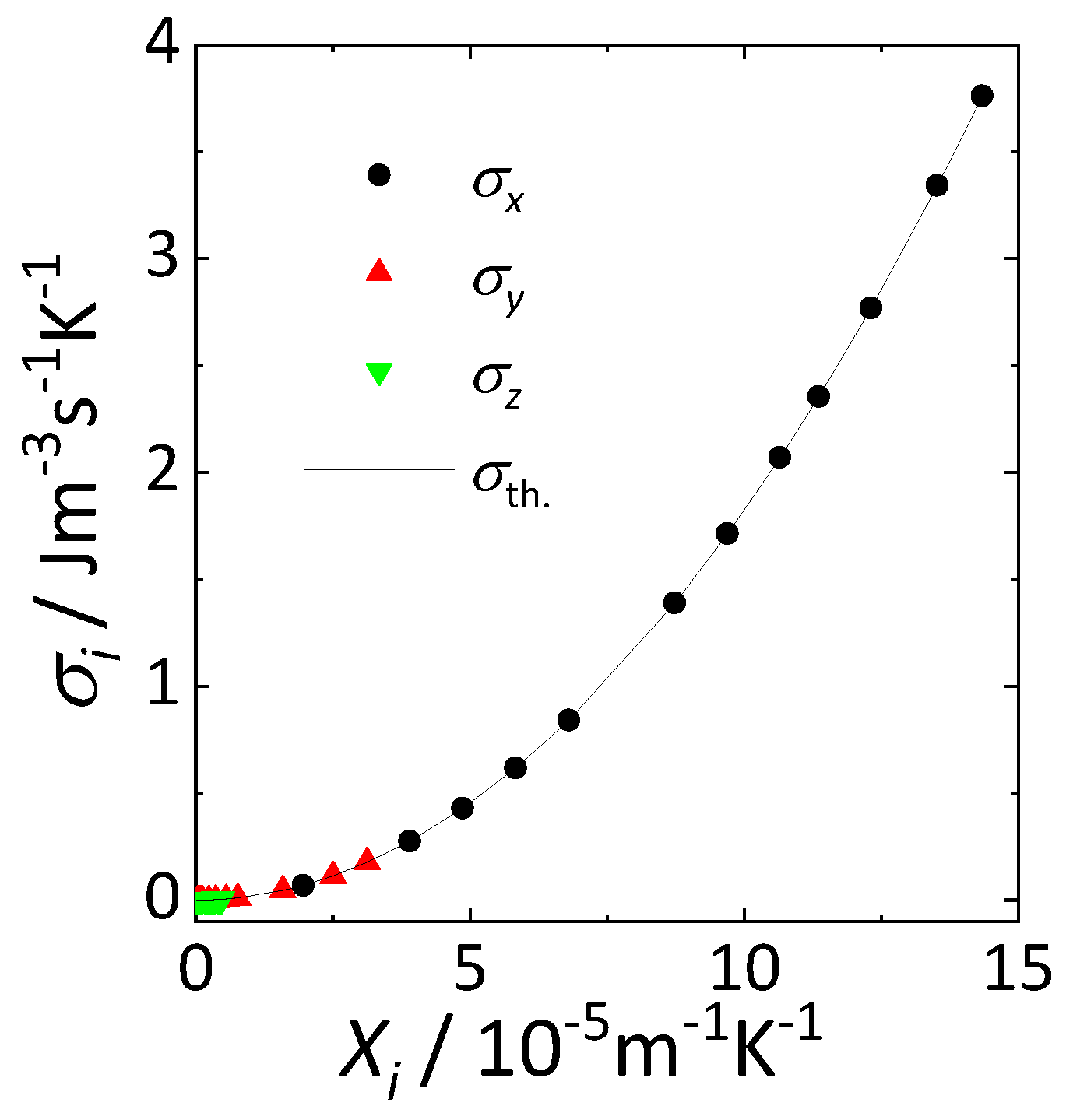
Figure 4.
Relationship between the heat fluxes and in the x- and y-directions, respectively, and the global driving force .
Figure 4.
Relationship between the heat fluxes and in the x- and y-directions, respectively, and the global driving force .
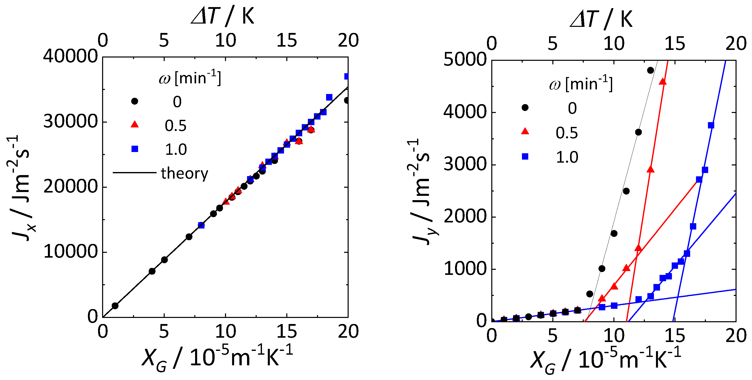
Figure 5.
Surface temperature fluctuations at (upper panel: HTW) and (lower panel: HTW). In the upper and lower panels, time progresses from left to right panel at intervals of 0.2 and 0.6 s, respectively.
Figure 5.
Surface temperature fluctuations at (upper panel: HTW) and (lower panel: HTW). In the upper and lower panels, time progresses from left to right panel at intervals of 0.2 and 0.6 s, respectively.
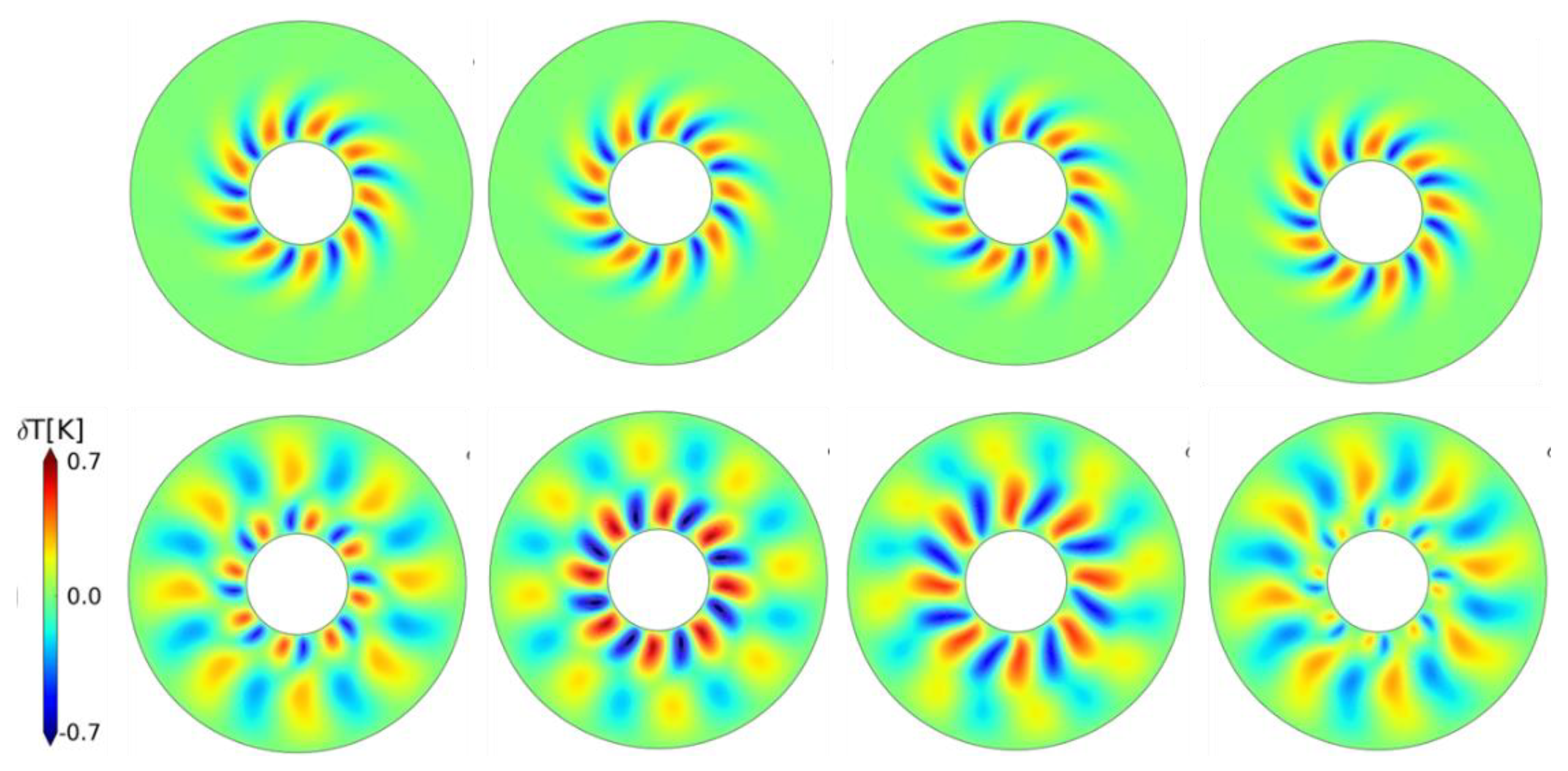
Figure 6.
Relationship between the heat flux , entropy generation , and the global driving force at . The black and red curves were fitted using Equations (12) and (13). The arrows indicate transition points.
Figure 6.
Relationship between the heat flux , entropy generation , and the global driving force at . The black and red curves were fitted using Equations (12) and (13). The arrows indicate transition points.
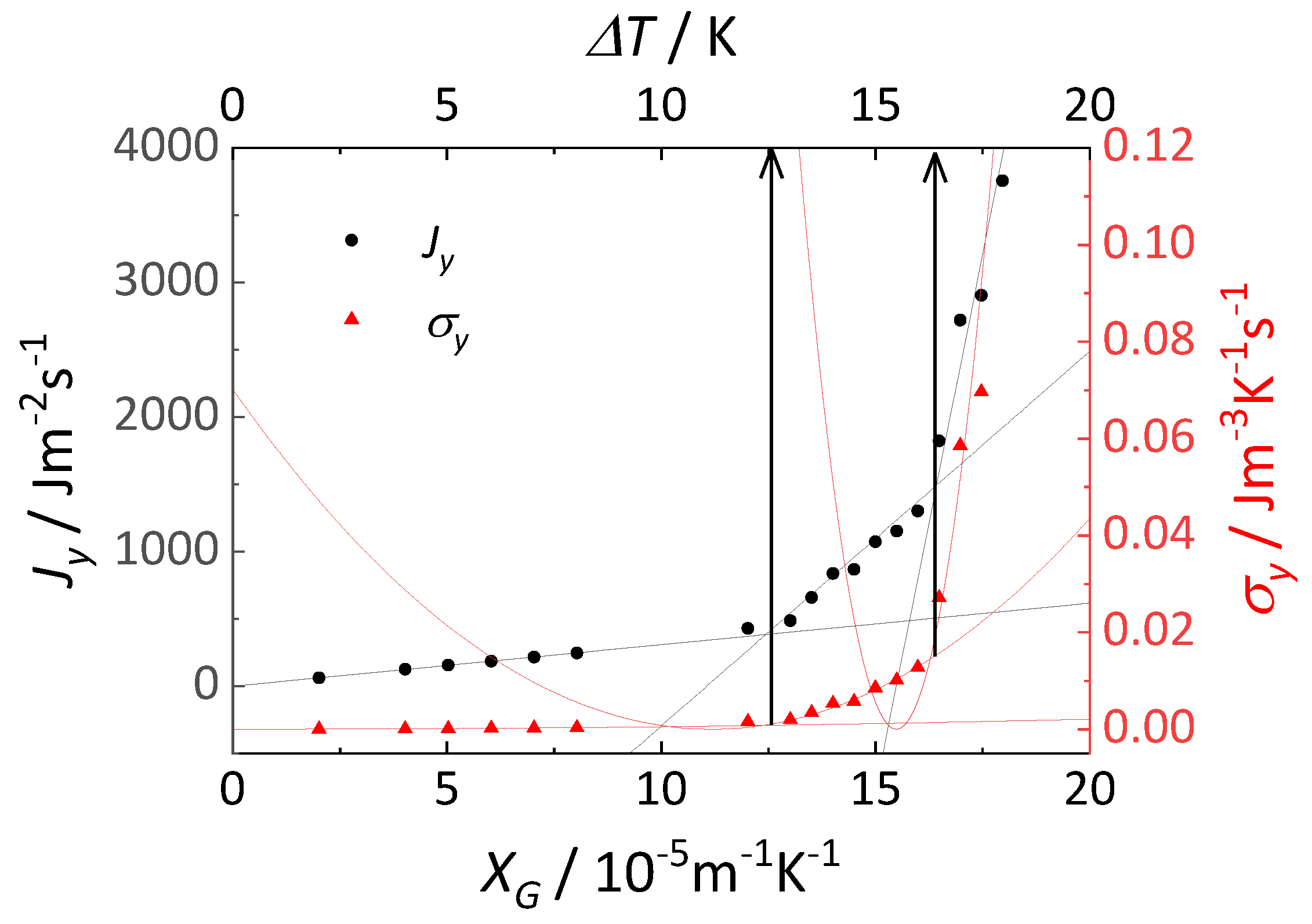
Figure 7.
(a) Temperature dependence of the chemical potentials of the three phases of matter in equilibrium. (b) Changes in emergent flux with global driving force for three different states of the system in nonequilibrium.
Figure 7.
(a) Temperature dependence of the chemical potentials of the three phases of matter in equilibrium. (b) Changes in emergent flux with global driving force for three different states of the system in nonequilibrium.
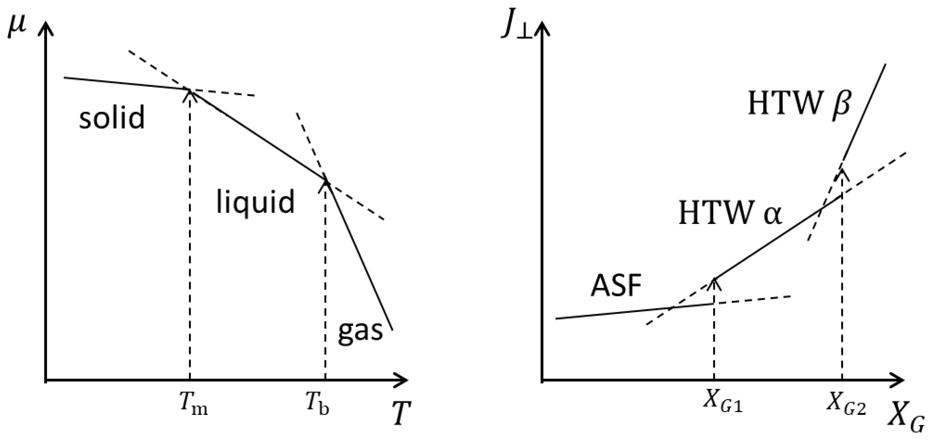

Table 1.
Physical properties of silicon melt.
| Physical properties | Value |
|---|---|
| Thermal conductivity () Viscosity () Density () Thermal expansion coefficient () Surface tension coefficient () Heat capacity () Melting temperature () |
64 Wm-1K-1 7.0×10⁻⁴ kgm-1s-1 2530 kgm-3 1.5×10⁻⁴ K-1 −7.0×10⁻⁵ Nm-1K-1 1000 Jkg-1K-1 1683 K |
Table 2.
Fitting parameters using Equations (12) and (13) at .
| Region | ||||||
|---|---|---|---|---|---|---|
| 1. 2. 3. |
|
|
|
|
|
|
Disclaimer/Publisher’s Note: The statements, opinions and data contained in all publications are solely those of the individual author(s) and contributor(s) and not of MDPI and/or the editor(s). MDPI and/or the editor(s) disclaim responsibility for any injury to people or property resulting from any ideas, methods, instructions or products referred to in the content. |
© 2024 by the authors. Licensee MDPI, Basel, Switzerland. This article is an open access article distributed under the terms and conditions of the Creative Commons Attribution (CC BY) license (http://creativecommons.org/licenses/by/4.0/).
Copyright: This open access article is published under a Creative Commons CC BY 4.0 license, which permit the free download, distribution, and reuse, provided that the author and preprint are cited in any reuse.


