
Submitted:
13 August 2024
Posted:
14 August 2024
You are already at the latest version
Abstract
Traditional painting artefacts study and documentation face the limitations of well-known recording tools and methods, such as handwritten or digital descriptions, scaled 2D drawings in situ, measurements with calipers, rulers or tape measures, sketches, tracings, as well as conventional or technical photographs. This paper advocates Close-Range Photogrammetry (SfM-MVS) and Reflectance Transformation Imaging (RTI) for recording vital morphological and 2.5D geometric features of painted surfaces with high accuracy. These digital tools, widely accessible due to increased computing power, enhance art observation, material study and conservation assessment. Despite specialized alternatives like 3D laser scanners, the focus here is on the cost-effective SfM-MVS and RTI, which offer advanced pixel colour accuracy. The ability to reproduce photorealistic textures proves essential for accurate documentation of painted artefacts. The paper showcases promising results from applying these methods to a mural from the Palace of Tiryns, justifying their fundamental role in an integrated scientific art study methodology.
Keywords:
2.5D imaging
; (SfM) structure from motion Photogrammetry
; (MVS) multi-view stereo
; (RTI) reflectance transformation imaging
; heritage documentation
; painting conservation
1. Introduction
The current research project emerged as elementary step of a fundamental workflow during the preparation of a PhD thesis on “Development of a methodology for the digital reconstruction of unreadable Bronze Age wall paintings using non-destructive physico-chemical methods and instrumental chemical analysis” at the Department of Conservation of Works of Art and Antiquities, University of West Attica, Greece. During the study of painted surfaces, the necessity for a geometrically precise digital reference model emerged to overlay visual 2D information from various electromagnetic spectrum ranges. This digital model, in the form of a 2.5D representation, must accurately depict shape, dimensions, color, texture, surface relief, and patterns without geometric distortions. Accurate geometric measurements and surface topography are vital for the study, understanding, and interpretation of works of art. The complexity, sensitivity, high value, and uniqueness of these artworks often limit the feasibility of extensive measurements and physical contact.
Previous research in recording and computing the 3D surfaces of painted artifacts has employed various methods, including 3D laser scanning and structured light scanning systems, to capture surface textures with sub-millimeter accuracy. These methods have yielded significant findings in geometric accuracy and surface topography but also present limitations in cost and accessibility.
This paper presents the application of SfM-MVS and RTI on a painted lime plaster fragment from the Palace of Tiryns, room 18 (Small Megaron) LHIIIB 2 (late 13th century BC), catalogued as MN33460 and housed in the Archaeological Museum of Nafplion (Peloponnese, Greece) (Rodenwaldt, 1912; Thaler, 2018). The aim is to create an accurate 3D model and a full-scale ortho-image (scale 1:1), as well as the detailed recording of the surface relief.
The next steps involve acquiring comprehensive optical 2D information across various regions of the electromagnetic spectrum and superimposing these images as layers, with pixel-level accuracy, onto the geometrically defined digital reference background produced by the SfM-MVS application. This substrate will be a 2.5D digital model, precisely defined in terms of shape and dimensions, free of geometric distortions. Combined with the complementary images from the RTI application, this model will accurately render the colour, texture, surface relief, and pattern of the painting.
However, the research process is still ongoing to fully exploit the potential of these techniques. Due to the so far absence of research data from the physicochemical study of the murals, in this project, the wall painting in question will not be presented in detail. It will serve as a case study for the application of SfM-MVS and RTI.
These methods were chosen because of their cost-efficiency and ability to provide accurate 3D models and photorealistic textures. They are proposed to become the essential tools in any typical workflow for the scientific study of painted artifacts.
2. Methodology
The main objective is to propose the coupling of two novel digital tools that have been developed in recent years and, along with the increase in computing power of personal computers, they have become widely available. These are Close-Range Photogrammetry exploiting structure-from-motion (SfM) and multi-view stereo (MVS) algorithms, and Reflectance Transformation Imaging (RTI) which, through the recording and computing of the third dimension of the painted surface, can provide a wide range of high-resolution spatial and colour information that is crucial for the viewing and the understanding experience by an observer or art historian, the study of the materials and the construction technique by a researcher, the recording of the present and ongoing state of preservation by an art conservator or the management of the object by a curator when planning an exhibition.
2.1. Photogrammetry
SfM photogrammetry is a passive, (Kraus, 2007, p. 413, 414; Remondino & El-Hakim, 2006) image-based documentation technique that allows the derivation of accurate, metric and semantic information from a series of digital photographic images taken with off-the-shelf digital photographic equipment, but processed in specialist photogrammetry software (Kelley & Wood, 2018, p. 15). However, SfM differs fundamentally from conventional photogrammetry, as the geometry of the scene, camera positions and orientation are solved automatically without the need to specify a priori a network of targets that have 3-D positions known in advance. Instead, these are solved simultaneously using a highly redundant, iterative bundle adjustment procedure, based on a database of features automatically extracted from a set of multiple overlapping images (Westoby et al., 2012). It rigorously turns 2D image data into 3D data (like digital 3D models) establishing the geometric relationship between the acquired images and the scene as surveyed at the time of the imaging event (Remondino & Campana, 2014, p. 65). Since it is a passive technique with no emitting light, it relies purely on natural illumination, and in that way does not physically harm the object material (Fuhrmann et al., 2014). Even though the term SfM photogrammetry is only part of the obtaining 3D models from overlapping pictures process, it is also widely used to denote a photogrammetry methodology (Iglhaut et al., 2019; Solem& Nau, 2020).
The procedure followed in this project was to capture a series of images, from multiple angles, with over 75% overlap, and load them into Agisoft Metashape Pro, the commercial, user-friendly computer vision-based software package, to generate a textured 3D model and subsequently achieve the ortho-projection of the painting surface. The process is referred to as Structure-from-Motion (SfM) (Ullman, 1976) and Multi-View Stereo (MVS) (Furukawa & Hernández, 2015) photogrammetry.
SfM is considered an extension of stereo vision. Instead of image pairs the method attempts to reconstruct depth from several unordered 2D images that depict a static scene or an object from arbitrary viewpoints. It relies on computer vision algorithms that detect and describe local interest points for each image (i.e., image locations that are in a certain way exceptional and are locally surrounded by distinctive texture) and then match those 2D interest points throughout the multiple images. This results in a number of potential correspondences (often called tie points). Using this set of correspondences as input, SfM computes the locations of those interest points in a local coordinate frame and produces a sparse 3D point cloud that represents the geometrical structure of the scene (Verhoeven et al., 2013). Inherently, the scale, position, and orientation of any photogrammetric model are arbitrary (Barnes, 2018). For the outputs to be scaled and their dimensions to be measurable, it is necessary to define the relationship between the image and the coordinates of the object. For this purpose, it is essential to place at least three control points (CPs) or GCPs (a GCP is a point on the object illustrated in the image, while at the same time, its 3D coordinates (X, Y, Z) are known, either in a local or in a global reference system) with the exact known distances between them or certified scale-bars established at appropriately selected positions within the photographed scene. The accuracy of the reference information that is used to scale the photogrammetric model will determine the scale accuracy of any data output. After the reconstruction of the 1:1 scale photogrammetric model is made, any measurement or study of the model can be obtained without limitations regarding the place, as the physical presence in situ/where the original object is located, is not necessary.
SfM photogrammetry as a passive image-based technique, the results are heavily influenced by the input image data. Employing an automated process to identify and match features by computer vision, is fundamentally dependent on the image quality. That being said, any sensors, settings and acquisition designs should be considered with great care.
2.1.1. Data Acquisition
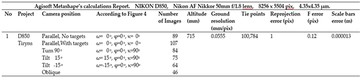
The present photogrammetric survey was carried out using a Nikon D850, Full-Frame 45.7MP Single-Lens Reflex Digital camera with a CMOS sensor (8256 x 5504 pixels, 4,35μm pixel size) equipped with a Nikon AF Nikkor 50mm f/1.8 lens.
In total, 468 images (Figure 1, Figure 2 and Figure 3) in RAW (NEF) format and 16-bit depth were captured by the Nikon D850 camera tethered to a laptop. The mural was placed horizontally on a tray on the floor. The camera was mounted at a distance of 715mm from the painting, on a custom-made construction of a device allowing fully controlled manual movement along the x and y axes, with horizontal marking to ensure precise movement distance while parallel to the painting surface, achieving constant focus throughout the entire shooting process. 139 images were taken at a small angle of about 15° and -15° to the horizontal plane (Figure 2) and 49 images at a larger angle around the mural (Figure 3) in order to contribute to the creation of the 3D model [1,2,3] keeping constant the focus and distance from the object. More specifically, in a coordinate system where the three camera rotation angles are according to Figure 4, the images acquired were as follows: 196 images with ω=0 o, φ=0 o, κ=0 o, 84 images with ω=0 o, φ=0 o, κ=90o (Figure 1 and Figure 2), 75 images taken with the camera tilted at an angle of ω= +15 o and 64 additional images taken with the camera tilted at an angle of ω= -15 o (Figure 1, Figure 2, Figure 3 and Figure 4) to the centre of the mural. A baseline (i.e., the distance between photography positions) of ca. 100mm and 100mm along the x and y axes allowed an overlap of ca 79% in longitudinal movement and ca 69% in lateral movement according to the equations (1, 2) (Figure 5). Two Speedlight flashes in softboxes were chosen as a light source, oriented downwards at an angle of 45° to the surface of the wall painting, ensuring uniform illumination and avoiding strong shadows. The use of Speedlight flashes was chosen because they provided adequate lighting conditions ensuring controlled colour balance, fast shutter speeds of 1/100, closed aperture of f/8 (medium f-number) and ISO 100. The two flashes were automatically triggered by the camera using a wireless transmitter at ¼ +0.7 of power.
SA= 318mm (image lateral length)
A= 100mm (lateral movement)
q= (lateral overlap)
q≈ 68.5% overlap
SB= 473mm (image longitudinal length)
B= 100mm (longitudinal movement)
p= (longitudinal overlap)
p≈78.8% overlap
So, the overlap in y axis is q≈68.5% and in x axis is p≈78.8% for each position of the camera
To establish the reference system, 16 coded targets (calibrated Agisoft’s markers) (Figure 6 and Figure 7) were placed in the subject’s frame. Target placement locations were chosen to be in areas of low interest on a neutral background of the painting’s surface, as well as in 4 fixed locations outside the mural. The target locations outside the mural consist of custom-made 90o angle rulers with prefabricated coded pears of Metashape targets with known highly accurate pre-measured distances in between. They have been located in such a way that the rulers on each side should form a straight line and be levelled at a plane consisting of the coded targets (5, 1, 7) (Figure 6) and the painted surface of the mural. By knowing precisely, the distance between two discrete points, referred to as Scale Bars, Agisoft Metashape is able to transform the spatial data of the model into real-world dimensions and create a 1:1 exact scaled photogrammetric model. Moreover, the software reads metadata from the camera and lens and, while carrying out the Align Photo procedure, estimates both interior and exterior camera orientation parameters, including nonlinear radial distortions (Agisoft, 2023). Due to the SfM algorithm, it can automatically estimate the camera’s calibration parameters for a known focal length (f) or principal distance (c) of the utilized lens. This method, is called self-calibration. While self-calibration in Agisoft Metashape can provide accurate results in many cases, for critical applications where high accuracy is required, it’s often recommended to perform a manual calibration by photographing a calibration pattern instead. The camera-lens calibration procedure followed in Agisoft Metashape involved taking 21 photographs of the checkerboard calibration pattern displayed on the LCD screen with the camera from slightly different angles. These images were captured with the same camera, lens, and focal length settings as when photographing the mural in situ. By importing these images into Metashape as a separate chunk and performing camera calibration during the editing workflow, the stored calibration data participated in the photo-alignment process.
For any digital photogrammetric project, the potential density of measurements and precision with which any individual measurement can be made, are going to be partially connected to
- the distance from the camera to the object (H),
- the sensor’s natural size (ps)/resolution of the camera, and
- the focal length of the lens (c).
These three variables together determine the size that any given pixel in an image occupies on the surface of the subject being imaged. This value, equal to the distance between the centre of two adjacent pixels as measured on the subject’s surface, is known as ground sample distance (GSD) (Barnes, 2018).
So, according to the equation (Stylianidis & Remondino, 2016, p. 264)
c=50mm, ps=4,35μm, H=715mm
According to equation (7)
(Agisoft calculates it to be equal to 0.055mm, Table 1)
This means that in order to achieve a GSD of less than 0.058 mm with the specific camera and lens, the images should be captured from a distance of less than 715 mm from the object.
According to (Verhoeven, 2018)
ps or p: photosite, detector pitch (μm)
H or s: object distance from optical centre (mm)
f’: focal length of the lens
w: sensor width
W: footprint width, the object space that is captured by the imaging sensor in the same aspect ratio
According to (Patias & Karras, 1995, p. 46)
For H=715mm and f=50mm (focal length)
Then
So, according to (Hecht, 2017, p167; Stylianides & Remondino, 2016, p. 167), c=f only when H= ∞
2.1.2. Data Processing
After the sequence of image capture was completed, Adobe Photoshop Lightroom Classic software (12.3 Release) was utilized to adjust the white balance based on the colour calibration chart X-Rite Colorchecker® Passport Photo target (in order to relate the recorded colours to the well-defined standards of ICC profiles) and applied to all images via sync. Finally, the RAW files were batch processed [2] into DNG uncompressed format in Adobe Photoshop software (24.4.1 Release).
The next step was to import all images into Agisoft Metashape Pro to generate the 3D models (Table 1). This semi-automated process consisted of seven basic consecutive steps: Align Photos, Build Mesh (3D polygonal model), Build Texture, Build Point Cloud, Build DEM, Build Orthomosaic and Export Results. A detailed step-by-step guide to the software procedure is presented in the Agisoft Metashape Pro manual. The Build Texture step, which generates the colour texture map, was performed with 89 images taken parallel to the surface before placing the coded targets so that the surface of the model to be generated was not covered by the targets.
2.2. Reflectance Transformation Imaging Technique RTI
RTI is a computational photographic method (Frey et al., 2011, p. 125) that captures the relief of the object’s surface through highlights and shadows in situ, taking advantage of the ability to relight the subject interactively and virtually in real-time from various angles at the office. It describes a suite of technologies and methods for generating surface reflectance information using photometric stereo i.e., by comparison between images with fixed camera and object locations but varying lighting (Woodham, 1980). RTI refers to a file format (Mudge et al., 2006) in addition to a set of methods. The most common implementation of RTI is via Polynomial Texture Mapping (PTM) fitting algorithm, invented by Tom Malzbender of HPLabs (Earl et al., 2010; Malzbender et al., 2001; 2000). PTM is a mathematical model describing luminance information for each pixel in an image in terms of a function representing the direction of incident illumination. The illumination direction function is approximated in the form of a biquadratic polynomial whose six coefficients are stored along with the colour information of each pixel (Zanyi et al., 2007).
RTI is a non-invasive/non-contact method that has its roots in the principles of raking illumination (Frey et al., 2011, p. 116; Alexopoulou-Agoranou, A. & Chrysoulakis, 1993, p. 127-129) that has been extensively used in museums and other heritage contexts. A raking light photograph is made by casting light across the surface of a painting at a very low angle, highlighting any surface texture or irregularities, including incisions, impasto, raised or flaking paint, damages and deformations of the canvas or panel. However, as photographs are usually taken with lights in only one, or perhaps two, positions, the information obtained depends largely on the choice of lighting position; a photograph with lights designed to highlight a particular area may not reveal interesting features in another part of a painting (Padfield et al., 2005, p. 1). PTM overcomes this drawback by allowing virtual re-lighting of the subject from any direction and subsequently through the mathematical enhancement of the shape and colour subsequently attributes of the object’s surface reveal information about the topology and reflection of the imaged surface in the form of surface “normal” (Woodham, 1980) for each pixel (Frank, 2014a; Hewlett-Packard, 2009; MacDonald & Robson, 2010; Malzbender et al., 2001; Schädel, 2022). This “normal” information indicates the directional vector’s perpendicular to the subject’s surface at each location recorded by the corresponding image pixel. Since each encoded normal corresponds to a point on the object, the whole set provides a complete and accurate “description” of its topography. Consequently, PTMs are 2D images containing true 3D information. This ability to document colour and true 3D shape information by using normals, is the source of RTI’s documentary power (Happa et al., 2010). The enhancement functions of RTI reveal surface information that is not readily discernable under direct empirical examination of the physical object. Today’s RTI software and related methodologies were constructed by a team of international developers.
Each RTI resembles a single, two-dimensional (2D) photographic image. Unlike a typical photograph, reflectance information is derived from the three-dimensional (3D) shape of the image subject and encoded in the image per pixel, so that the synthesized RTI image “knows” how light will reflect off the subject. When the RTI is opened in RTIViewer software, each constituent pixel can reflect the software’s interactive “virtual” light from any position selected by the user. This changing interplay of light and shadow in the image discloses fine details of the subject’s 3D surface form (Cultural Heritage Imaging, 2002-2021). The interactive output is produced from multiple photographs that are taken from one stationary position, while the surface of the subject is illuminated from different raking light positions in each shot. Although this is technically a 2D recording approach, it is often described as 2.5D because of the high-level visual information provided by highlighting and shadowing 3D surfaces. It should be noted that this procedure, as described, although providing detailed qualitative surface information, does not produce metrically-accurate 3D data (Historic England, 2018).
There are several capture methods that can be utilized to create a PTM, each requiring different tool kits and budgets. Because of the relatively inexpensive, transportable tool kit and flexible recording parameters, the Highlight-RTI or H-RTI method was chosen for this project. H-RTI image capture is a technique that permits the capture of the light position as the photo is shot obtaining the digital image data from which you can produce reflectance transformation images (RTIs). An RTI, in addition to storing the colour data for each pixel, stores a “normal” value for each pixel that records its surface shape. The processing software calculates this value using data about the position of the light in each image, relative to the camera.
A key element of the RTI methodology is the presence of one or (preferable) two reflective black glossy spheres in the frame of the photograph in each shot. The reflection of the light source on the spheres, in each image, enables the processing software to calculate the exact light direction for that image. The size of the spheres depends on the dimensions of the object being photographed and the resolution of the camera. It must be noted that the sphere diameter should be at least 250 pixels wide to be fine for RTI calculation. As with the various camera setups, the sphere configuration needs to be adjusted according to the circumstances of the subject and environment. The appropriate position for the spheres can be determined by looking at the camera’s view.
During post-processing, the reflective spheres will be cropped out from the images; this is something to keep in mind when positioning them. They must be close enough to the subject so that the camera can focus on both the spheres and the subject with sufficient Depth of Field (DoF), but far away enough so that they can be cropped out of the image without losing any image data for the subject itself. It is very important to pay extreme attention during the shooting sequence so that the camera, the target object and the reflective spheres do not move at all - only the light “moves” (Cultural Heritage Imaging, 2013).
2.2.1. Data Acquisition
In total,32 lossless RAW (NEF) format photographs were taken with a Nikon Z6 Full-Frame, 24.5MP mirrorless camera equipped with a Tokina AT-X PRO SD 16-28mm f/2.8 (IF) FX lens shooting at 28mm focal length, mounted in a fixed position throughout the process, with the camera sensor parallel to the surface of the painting. The camera was tethered to a laptop via the USB computer-control cable so that it could be remotely triggered via Adobe Lightroom software. This layout enabled the camera viewfinder to be remotely displayed in a live-view mode on the larger screen of the laptop, providing the advantage of avoiding any possible movement of the camera while shooting, having better control of the photo frame, focus, brightness or white balance, as well as checking the quality of the captured images and saving them directly on the laptop’s hard drive. A Speedlight flash was employed as the light source, along 8 positions of an imaginary dome, at a fixed distance from the centre of the painting surface, positioned for each shot in 10-degree increments from the lowest angle of 10 degrees to the highest angle of 40 degrees. It was automatically triggered by the camera using a wireless transmitter. The use of a flash unit exposes the Mycenaean frescoes to relatively minimal levels of ultraviolet light and allows the image to be captured in 1/100 s at f/8 in ISO 100 (shutter speed 1/100, aperture f/8 and ISO 100).
The quality of the final RTI is based on the quality of the captured images. Although the processing software is relatively robust and photographing in RAW format allows for some post-processing adjustments, it is important to precede test shots with a grey card to select the appropriate exposure (aperture, shutter speed and light intensity from the light source) by examining the histogram of the captured images. This process, at the time of analogue photography, would require the use of a photometer.
It is also recommended that before each capture sequence or during the shooting, a shot be taken using the light source at the highest angle (65 degrees) with a colour balance card incorporated in the subject’s frame (Cultural Heritage Imaging, 2013). This image capture will be used later in the post-processing phase to adjust the colour of the photographs and ensure accurate colour by compensating for the effects of the colour temperature of the light source (Historic England, 2018). The colour balance card that has been used was contained in the X-Rite Colorchecker® Passport (Frey et al., 2011, p. 93).
2.2.2. Data Processing
After the acquisition of the images was complete, Adobe Lightroom software was used to make appropriate white balance adjustments based on Colorchecker® Passport, which was applied to all images via synchronization. Finally, the RAW files were batch-processed into DNG format and then converted to JPEG (.jpg) in Adobe Photoshop software. Tethered shooting and data processing for both techniques Close-Range Photogrammetry (SfM-MVS) and Reflectance Transformation Imaging (RTI) was performed by a Microsoft Surface Studio laptop with a Quad-core Intel 11th Gen Intel Core H35 i7-11370H@ 3.30GHz, 32GB LPDDR memory (4 x 32 GB), 64-bit operating system (Windows 11) and 4GB GDDR6 GPU memory NVIDIA GeForce RTX 3050 Ti laptop graphics card.
Post-processing of the 32 image captures occurred through the open-source RTIBuilder software (Version 2.0.2.) and HSHfitter in order to collate information about the direction of the light source and generate the final RTI file. The generated RTI file was then loaded into RTIViewer software (Version 1.1) available from the CHI website.
3. Results
3.1. Photogrammetry Results
The outputs generated in the photogrammetric survey of the wall paintings are the Point cloud, the Dense elevation model (DEM) and the Orthomosaics.
The Point cloud consists of points in a three-dimensional space providing a detailed representation of the geometry of the mural (Figure 8, Figure 9, Figure 10 and Figure 11).
The produced Dense Elevation Model (DEM) is a 2.5D model (Figure 12) of the surface which uses pixel locations to represent X and Y coordinates, and pixel values to represent the depth. The colour gradient corresponds to measurable altitudinal gradients. They can also be visualized in the form of elevation contours (Figure 13). Metashape also enables the calculation of cross sections with the cut being made at a plane parallel to the z-axis (Figure 14 and Figure 15).
Orthomosaics are usually high-resolution photomosaics (Figure 16) of numerous overlapping photographs and three-dimensional models (Figure 8, Figure 9, Figure 10 and Figure 11), providing a metric record of the paintings at a single point in time (Figure 18). The most utilized outputs are orthoimages (Figure 16 and Figure 17), which are rectified images that are corrected for most distortions (Granshaw, 2020).
The orthoimage is an image of the object surface in orthogonal parallel projection allowing measurement of distances, angles, areas etc. (Figure 17, Figure 18 and Figure 19) The orthogonal projection reflects a uniform scale in every product point since no relief displacements appear on the product. The orthoimage is divided into pixels by considering a specific pixel size based on the ground coordinate system. For each one of these pixels, a specific greyscale or RGB value corresponds. This value is obtained from the original image corresponding to the appropriate pixel, by using one of the resampling methods namely nearest neighbor, bilinear and bicubic (Stylianidis & Remondino, 2016).
3.2. RTI Results
The real power of this technique is the interactive RTI Viewer tool which allows the viewer to virtually relight the object’s surface from any direction, much like tilting it back and forth to catch the light and shadow that best reveal features of interest. Furthermore, its enhanced vision reveals shallow reliefs that may not be easily distinguishable under normal lighting conditions or by photogrammetry. However, the results and their interpretation are the subject of an ongoing research project. Therefore, to reach and present confident and reliable conclusions, the information obtained from these two methodologies in combination with other studies should be taken into account. Indicatively it can be mentioned that the application of the RTI methodology makes it possible to distinguish the painter’s brushstroke as well as the sequence of the colour layers, i.e., which of them was applied first and which last. That information may be suspected or assumed, but by the RTI, a non-contact, non-invasive technique, can be certified with certainty.
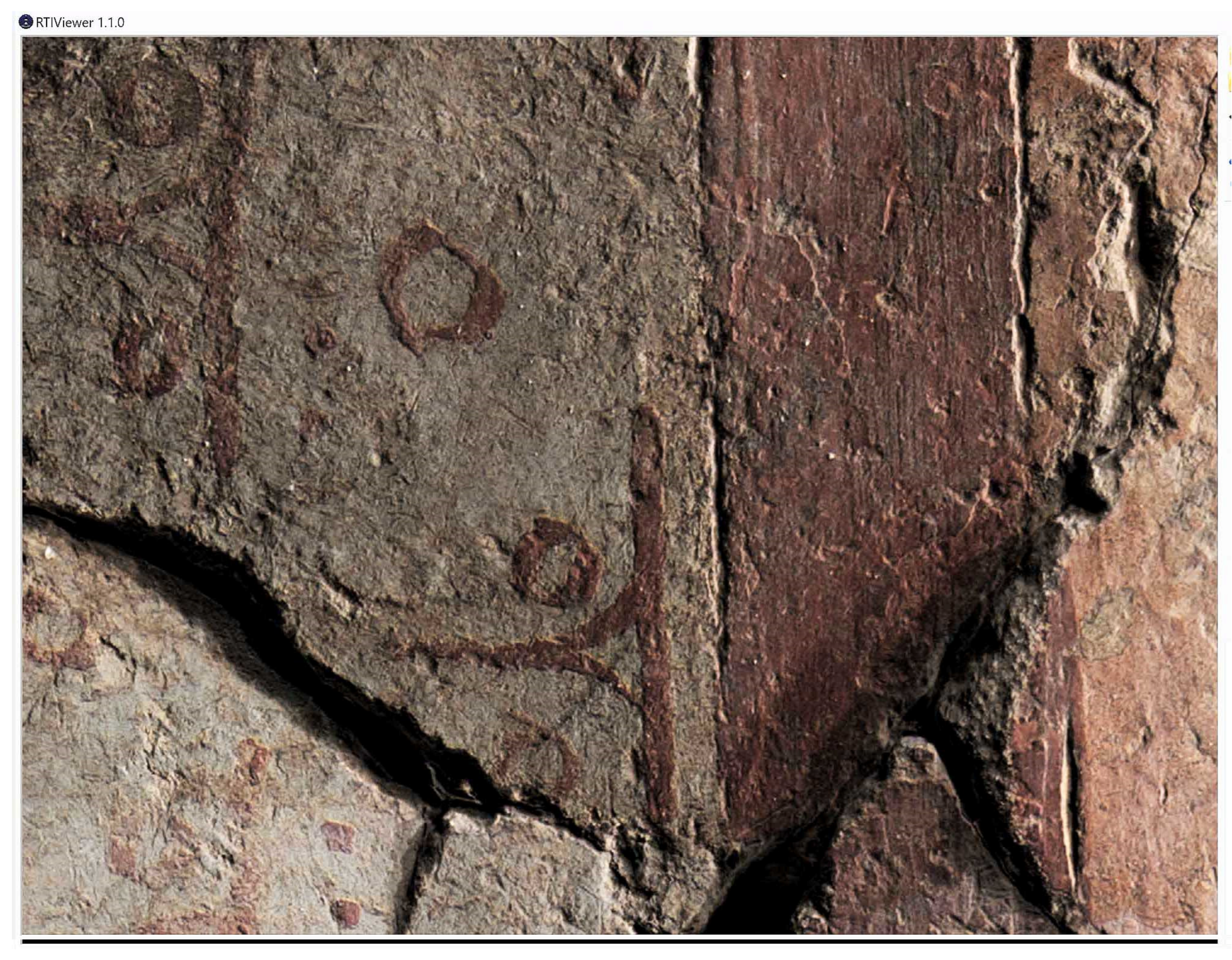
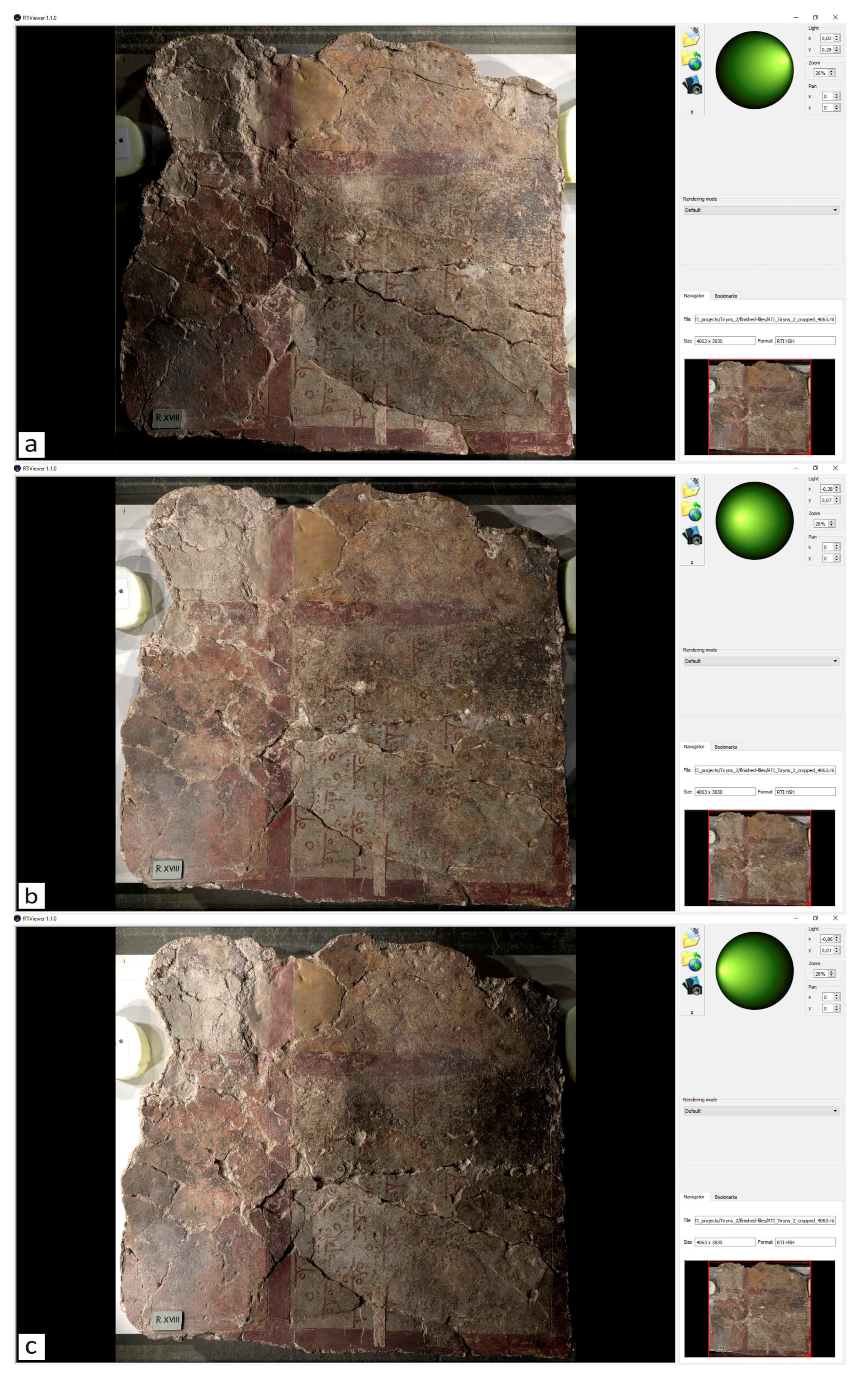
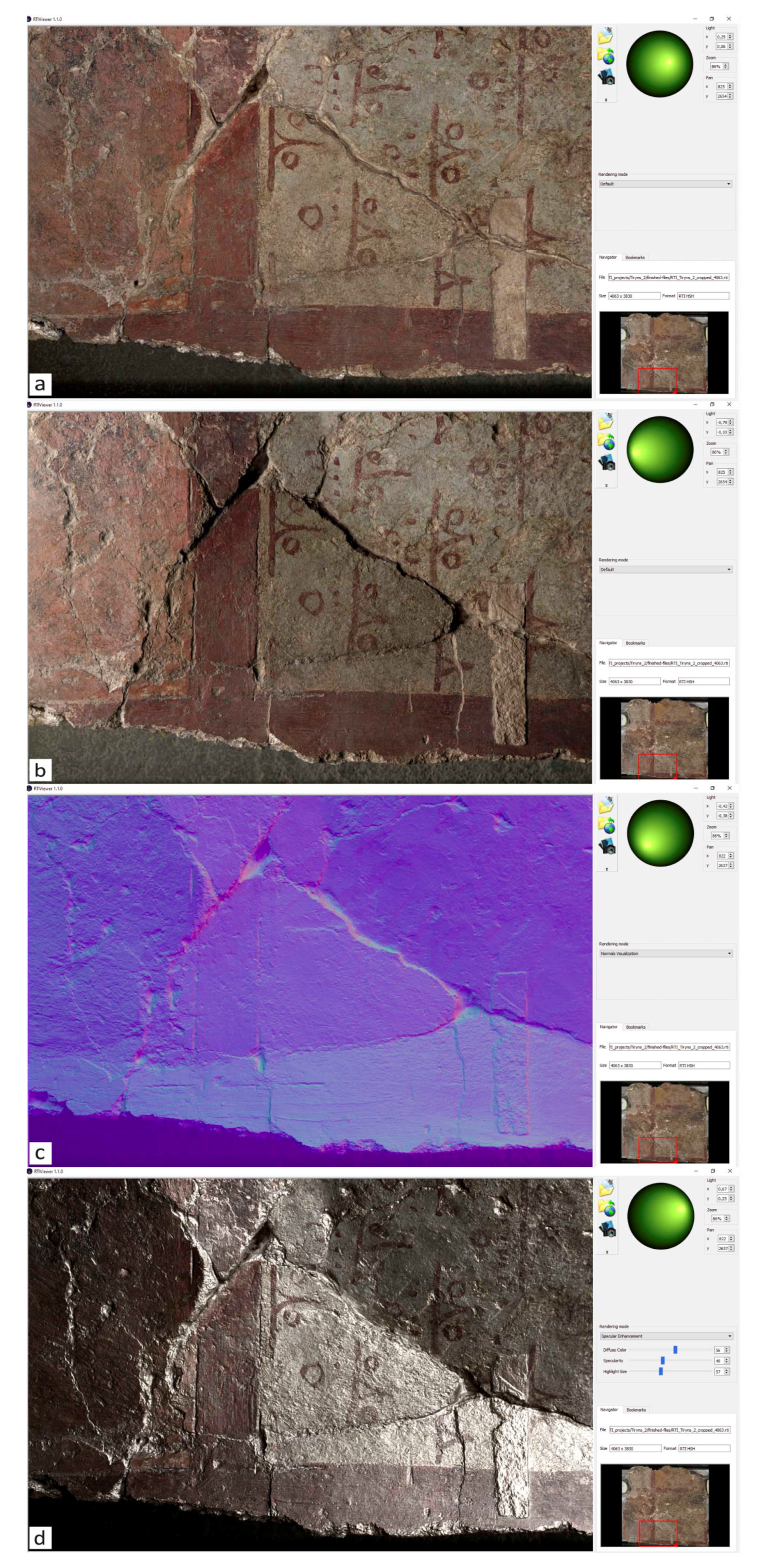
Figure 21.
RTIViewer screenshot. RTI highlights surface anomalies, damages, or irregularities on the painting surface.
Figure 21.
RTIViewer screenshot. RTI highlights surface anomalies, damages, or irregularities on the painting surface.
Figure 22.
a, b, c. RTIViewer screenshots with the green sphere (top right) adjusted in different direction of light.
Figure 22.
a, b, c. RTIViewer screenshots with the green sphere (top right) adjusted in different direction of light.
Figure 23.
a, b, c, d. Screenshots from RTIViewer. In (a) and (b) different directions of light enhance the topography information. In (c) we exploit the RTI Normals Visualization and in (d) string impressions are most clearly visible by the RTI-HSH specular enhancement.
Figure 23.
a, b, c, d. Screenshots from RTIViewer. In (a) and (b) different directions of light enhance the topography information. In (c) we exploit the RTI Normals Visualization and in (d) string impressions are most clearly visible by the RTI-HSH specular enhancement.
4. Conclusions
This paper aims to demonstrate the benefit of coupling Close-Range Photogrammetry (SfM-MVS) and Reflectance Transformation Imaging (RTI), as a standard workflow for the recording and documentation of painted works of art. These two methods are recommended as complementary techniques due to the distinct types of information they provide. Photogrammetry produces an accurate, geometrically defined 2.5D digital mural “twin” by capturing the actual relief of the painted surface. In contrast, RTI uses selective illumination to acquire controlled visual information, enabling virtual illumination on demand and the observation of shallow texture variations, which are mathematically enhanced to make them more distinct and legible. Furthermore, both methods can be implemented using consumer-grade cameras, which are affordable and widely available in conservation and research laboratories. This makes the techniques accessible to conservators and researchers with minimal technical expertise.
Digitally recording a painting with photogrammetry and RTI and creating the 2.5D model offer the unique ability to exploit depth information, significantly enhancing the study process. This approach overcomes limitations related to the object’s preservation status, exposure, storage location, available observation time, or object-observer distance. Regardless of where the physical object is located, its digital “twin”, (Grieves, 2015) can be accessed and studied from any location, providing the opportunity to examine it closely from a few centimeters away.
A digital replica allows for the observation of an entire scene or a focused area, down to the pixel level, collecting high-resolution spatial and color information. The model can be rotated, zoomed, and measured with absolute precision without physical contact with the original object. Τaking advantage of the ability to interactively virtually relight the subject in real-time from various angles in the RTIViewer environment, enhances the surface relief, revealing detailed information about construction techniques, colour layers, brushstroke textures, and the artist’s signature or fingerprint.
These techniques also facilitate the detection of micro-cracks, bulging, flaking, losses, and previous conservation-restoration interventions, which are often not visible to the naked eye. During conservation, they allow for three-dimensional recording of the stages of conservation, damages, or deformations during exhibition or storage, creating a valuable digital record of high geometric and imaging accuracy for future analysis.
The digital record can serve as a reference background for integrating layers or metadata, including images in different wavelengths, drawings, sketches, annotations, and notes. It forms a comprehensive and dynamic digital record that can be updated with new information or formulations in the future.
In conclusion, the application of these methods is highly promising, and the results justify their proposal as fundamental non-invasive recording tools in the regular workflow of a standardized and integrated scientific methodology for the documentation and study of works of art.
This project is an initial presentation of the methodology proposed for the creation of a geometrically accurate 3D model, a true digital replica, and a full-scale ortho-image (scale 1:1) of the mural under examination as well as the recording of the surface relief, the morphological and geometric characteristics of the colour layers and the brushstrokes relief utilizing the capabilities provided by Reflectance Transformation Imaging. The resulting orthophoto will serve as the geometrically defined background layer, onto which, imaging information from the hyperspectral analysis of the drawing technique and pigments, will be superimposed in layers.
Next steps involve acquiring optical 2D information across various regions of the electromagnetic spectrum and overlaying these images, with pixel-level accuracy, onto the digital reference background produced by the SfM-MVS application. This substrate will be a 2.5D digital model, precisely defined in shape and dimensions, free of geometric distortions. Combined with complementary RTI images, this model will accurately render the color, texture, surface relief, and pattern of the painting.
However, research is ongoing to fully exploit these techniques. Due to the current lack of physicochemical study data, a detailed presentation of the mural and an extensive interpretation of the information obtained from the application of SfM-MVS and RTI are not included in this project. Instead, the mural serves as a case study for the application of SfM-MVS and RTI.
Funding
This research did not receive any specific grant from funding agencies in the public, commercial, or not-for-profit sectors.
Acknowledgments
Grateful thanks to Dr Alkestis Papadimitriou Director of the Ephorate of Antiquities of Argolida for the permission to study the floor fragment with painted decoration from the Palace of Tiryns as well as for providing every assistance at the laboratories of the Ephorate in order to carry out this study. We also thank Aristides Stasinakis and Aristotelis Petrouleas for entrusting with some of the required photographic equipment and to Metrica S.A. for facilitating the supply of Agisoft Metashape Pro, the commercial software package.
List of Contributions
- Although parallel image acquisitions are good for human stereoscopic projection and automatic surface reconstruction, when combined with convergent acquisitions they often lead to higher accuracy, especially in the z-direction. (Linder, 2016, p11)
- The term “batch” refers to editing photos of an entire group of images rather than one image at a time, accelerating the editing process.
References
- Adamopoulos, E., Rinaudo, F., Ardissono, L., 2021. A Critical Comparison of 3D Digitization Techniques for Heritage Objects. ISPRS Int. J. Geo-Inf., 10, 10. https://doi.org/10.3390/ijgi10010010. [CrossRef]
- Agisoft LLC, 2023. Agisoft Metashape User Manual: Professional Edition, Version 2.0.
- Alexopoulou-Agoranou, A. & Chrysoulakis, G., 1993. Sciences and artworks, Ed. Gonis, Athens. (Published in Greek).
- Barnes, A., 2018. Digital Photogrammetry, in: López Varela, S.L. (Ed.), The Encyclopedia of Archaeological Sciences. John Wiley & Sons, Inc., Hoboken, NJ, USA, pp. 1–4. https://doi.org/10.1002/9781119188230.saseas0191. [CrossRef]
- Bianconi, F., Catalucci, S., Filippucci, M., 2017. “Comparison between two non-contact techniques for art digitalization”. Journal of Physics: Conference SeriesVol.882, No.1, IOP Publishing https://doi.org/10.1088/1742-6596/882/1/012005. [CrossRef]
- Cultural Heritage Imaging 2002-2021 https://culturalheritageimaging.org/Technologies/RTI/index.html.
- CHI, 2013. Reflectance Transformation Imaging. Guide to Highlight Image Capture v2.0.
- Earl, G., Beale, G., Martinez, K., & Pagi, H., 2010. Polynomial texture mapping and related imaging technologies for the recording, analysis and presentation of archaeological materials.
- Frank, E. B., 2014a. Documenting archaeological textiles with reflectance transformation imaging (RTI). Archaeological Textile Review 56, 3–13.
- Frey, F.S., Warda, J., American Institute for Conservation of Historic and Artistic Works (Eds.), 2011. The AIC guide to digital photography and conservation documentation, 2nd ed. ed. American Institute for Conservation of Historic and Artistic Works, Washington, D.C.
- Fuhrmann, S., Langguth, F., Goesele, M., 2014. MVE - A Multi-View Reconstruction Environment. Eurographics Workshop on Graphics and Cultural Heritage 8 pages. https://doi.org/10.2312/GCH.20141299. [CrossRef]
- Furukawa, Y., Hernández, C., 2015. Multi-View Stereo: A Tutorial. FNT in Computer Graphics and Vision 9, 1–148. https://doi.org/10.1561/0600000052. [CrossRef]
- Georgopoulos, A., 2016. Photogrammetric Automation: Is It Worth? https://doi.org/10.5281/ZENODO.204962. [CrossRef]
- Granshaw, S.I., 2020. Photogrammetric terminology: fourth edition. Photogram Rec 35, 143–288. https://doi.org/10.1111/phor.12314. [CrossRef]
- Happa, J., Mudge, M., Debattista, K., Artusi, A., Gonçalves, A., Chalmers, A., 2010. Illuminating the past: state of the art. Virtual Reality 14, 155–182. https://doi.org/10.1007/s10055-010-0154-x. [CrossRef]
- Hecht, E., 2017. Optics, 5 ed/fifth edition, global edition. ed. Pearson, Boston Columbus Indianapolis New York San Francisco Amsterdam Cape Town Dubai London Madrid Milan Munich.
- Hewlett-Packard, 2009. Polynomial texture mapping. http://www.hpl.hp.com/ research/ptm/index.html.
- Historic England, 2018. Multi-light Imaging for Cultural Heritage. Swindon: Historic England.
- Iglhaut, J., Cabo, C., Puliti, S., Piermattei, L., O’Connor, J., Rosette, J., 2019. Structure from Motion Photogrammetry in Forestry: A Review. Curr. For. Rep., 5, 155–168.
- International Council of Museums, 2005. ICOM Committee for Conservation: 14th Triennal meeting The Hague 12-16 September 2005. Vol. 1 (I. Verger, Ed.). James & James ; Earthscan.
- Ioannides, M., Fink, E., Brumana, R., Patias, P., Doulamis, A., Martins, J., Wallace, M. (Eds.), 2018. Digital Heritage. Progress in Cultural Heritage: Documentation, Preservation, and Protection: 7th International Conference, EuroMed 2018, Nicosia, Cyprus, October 29 – November 3, 2018, Proceedings, Part II, Lecture Notes in Computer Science. Springer International Publishing, Cham. https://doi.org/10.1007/978-3-030-01765-1. [CrossRef]
- Kelley, K., Wood, R. (Eds.), 2018. Digital imaging of artefacts: developments in methods and aims, Access archaeology. Archaeopress Publishing Ltd., Oxford.
- Koutsoudis, A., Vidmar, B., Ioannakis, G., Arnaoutoglou, F., Pavlidis, G., Chamzas, C., 2014. Multi-image 3DReconstruction Data Evaluation. Journal of Cultural Heritage 15: 73–79.
- Kraus, K., 2007. Photogrammetry: Geometry from Images and Laser Scans, 2nd [English] ed. Berlin – New York: Walter de Gruyter.
- Linder, W., 2016. Digital Photogrammetry. Springer Berlin Heidelberg, Berlin, Heidelberg. https://doi.org/10.1007/978-3-662-50463-5. [CrossRef]
- Luhmann, T., Robson, S., Kyle, S., Boehm, J., 2023. Close Range Photogrammetry and 3D Imaging.3rd., W. de Gruyter Verlag, Berlin, 852 p. https://doi.org/10.1515/9783111029672-202. [CrossRef]
- MacDonald, L.W., & Robson, S., 2010. Polynomial texture mapping and 3D representations.
- Malzbender, T., Gelb, D. and Wolters, H., 2001 Polynomial texture maps, In Proceedings of the 28th Annual Conference on Computer Graphics and Interactive Techniques, Los Angeles, CA, USA, 12–17, 519–528.
- Malzbender, T., Gelb, D., Wolters, H. & Zuckerman, B., 2000. Enhancement of shape perception by surface reflectance transformation. Hewlett-Packard Technical Report HPL-2000- 38.
- Mudge, M., Malzbender, T., Schroer, C. and Marlin, L., 2006. New reflection transformation imaging methods for rock art and multiple-viewpoint display. In Ioannides, M., Arnold, D., Niccolucci, F., Mania, K., European Association for Computer Graphics, ACM/Sig Graph, Technische Universität Graz, Technische Universität Braunschweig (Eds.), 2006. CIPA / VAST / EG / EuroMed 2006. Eurographics Association.
- Padfield, J., Saunders, D., Malzbender, T., 2005. Polynomial texture mapping: a new tool for examining the surface of paintings.
- Patias, P. & Karras, G., 1995. Modern Photogrammetric Practices in Architecture and Archaeology applications, Diptycho Publications, Thessaloniki, Greece. (Published in Greek).
- Petsa E., 2021-22. Photogrammetry I. (Introduction to Photogrammetry). Lecture Notes at the Photogrammetry & Computer Vision Laboratory-UNIWA. (Published in Greek).
- Petsa E., 2000. Fundamental Concepts and Fundamental Problems of Photogrammetry. (Published in Greek).
- Ray, S.F., 2002. Applied photographic optics: lenses and optical systems for photography, film, video, electronic imaging and digital imaging, Third edition. ed. Focal Press, Oxford ; Boston.
- Remondino, F., and Campana, S., 2014. 3D Recording and Modelling in Archaeology and Cultural Heritage Theory and best practices, In BAR International Series.
- Remondino, F., El-Hakim, S., 2006. Image-based 3D Modelling: A Review: Image-based 3D modelling: a review. The Photogrammetric Record 21, 269–291. https://doi.org/10.1111/j.1477-9730.2006.00383.x. [CrossRef]
- Rodenwaldt, G., 1912. Tiryns: die Ergebnisse der Ausgrabungen des Instituts (Band 2): Die Fresken des Palastes, Athens. https://doi.org/10.11588/diglit.1142#0001.
- Schädel, M., Yavorskaya, M., Beutel, R., 2022. The earliest beetle †Coleopsis archaica (Insecta: Coleoptera) – morphological re-eva luation using Reflectance Transformation Imaging (RTI) and phylogenetic assessment. ASP 80, 495–510. https://doi.org/10.3897/asp.80.e86582. [CrossRef]
- Stylianidis, E., Remondino, F. (Eds.), 2016. 3D recording, documentation and management of cultural heritage. Whittles Publishing, Caithness, Scotland, UK.
- Szeliski, R., 2022. Computer vision: algorithms and applications, Second edition. ed, Texts in computer science. Springer, Cham.
- Thaler, U., 2018. Mykene: Die sagenhafte Welt des Agamemnon, Katalog zur Ausstellung im Badischen Landesmuseum, 315.
- Ullman, S., 1979. The interpretation of structure from motion. Proceedings of the Royal Society of London. Series B. Biological Sciences, 203, 405 - 426.
- Verhoeven, G.J., Santner, M., Trinks, I., 2021. FROM 2D (TO 3D) TO 2.5D – NOT ALL GRIDDED DIGITAL SURFACES ARE CREATED EQUALLY. ISPRS Ann. Photogramm. Remote Sens. Spatial Inf. Sci. VIII-M-1–2021, 171–178. https://doi.org/10.5194/isprs-annals-VIII-M-1-2021-171-2021. [CrossRef]
- Verhoeven, G.J., 2018. Resolving Some Spatial Resolution Issues – Part 1: Between Line Pairs And Sampling Distance. https://doi.org/10.5281/ZENODO.1465017. [CrossRef]
- Verhoeven, G., Doneus, N., Doneus, M., & Štuhec, S., 2015. From pixel to mesh: accurate and straightforward 3D documentation of cultural heritage from the Cres/Lošinj archipelago. In Ettinger Starčić, Z., Tončinić, D. (Eds.), 2015. Istraživanja na otocima: znanstveni skup, Veli Lošinj, [1. do 4. listopada] 2012. god. Hrvatsko arheološko društvo : Lošinjski muzej, Zagreb, Mali Lošinj.
- Westoby, M.J., Brasington, J., Glasser, N.F., Hambrey, M.J., Reynolds, J.M., 2012. ‘Structure-from-Motion’ photogrammetry: A low-cost, effective tool for geoscience applications. Geomorphology 179, 300–314. https://doi.org/10.1016/j.geomorph.2012.08.021. [CrossRef]
- Woodham, R.J., 1980. Photometric Method For Determining Surface Orientation From Multiple Images. Opt. Eng 19. https://doi.org/10.1117/12.7972479. [CrossRef]
- Zányi, E., Schroer, C., Mudge, M., Chalmers, A., & Francisco, S., 2007. LIGHTING AND BYZANTINE GLASS TESSERAE.
Figure 1.
Camera positions during the photogrammetric survey. In total, 468 images in RAW (NEF) format were captured by the Nikon D850 camera.
Figure 1.
Camera positions during the photogrammetric survey. In total, 468 images in RAW (NEF) format were captured by the Nikon D850 camera.
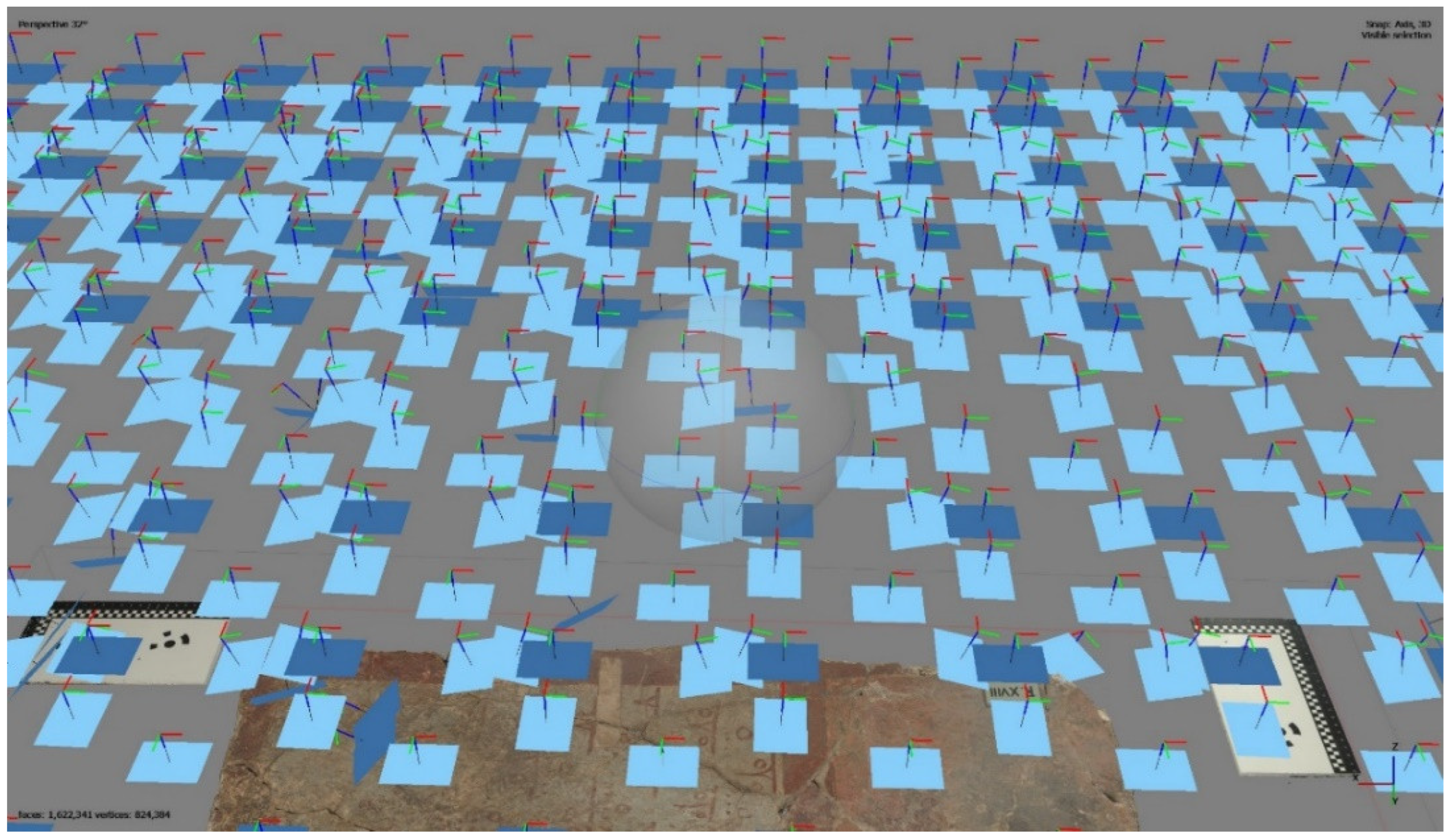
Figure 2.
Camera positions during the photogrammetric survey. 139 images were taken at a small angle of about 15° and -15° to the horizontal plane which is parallel to the painting surface.
Figure 2.
Camera positions during the photogrammetric survey. 139 images were taken at a small angle of about 15° and -15° to the horizontal plane which is parallel to the painting surface.
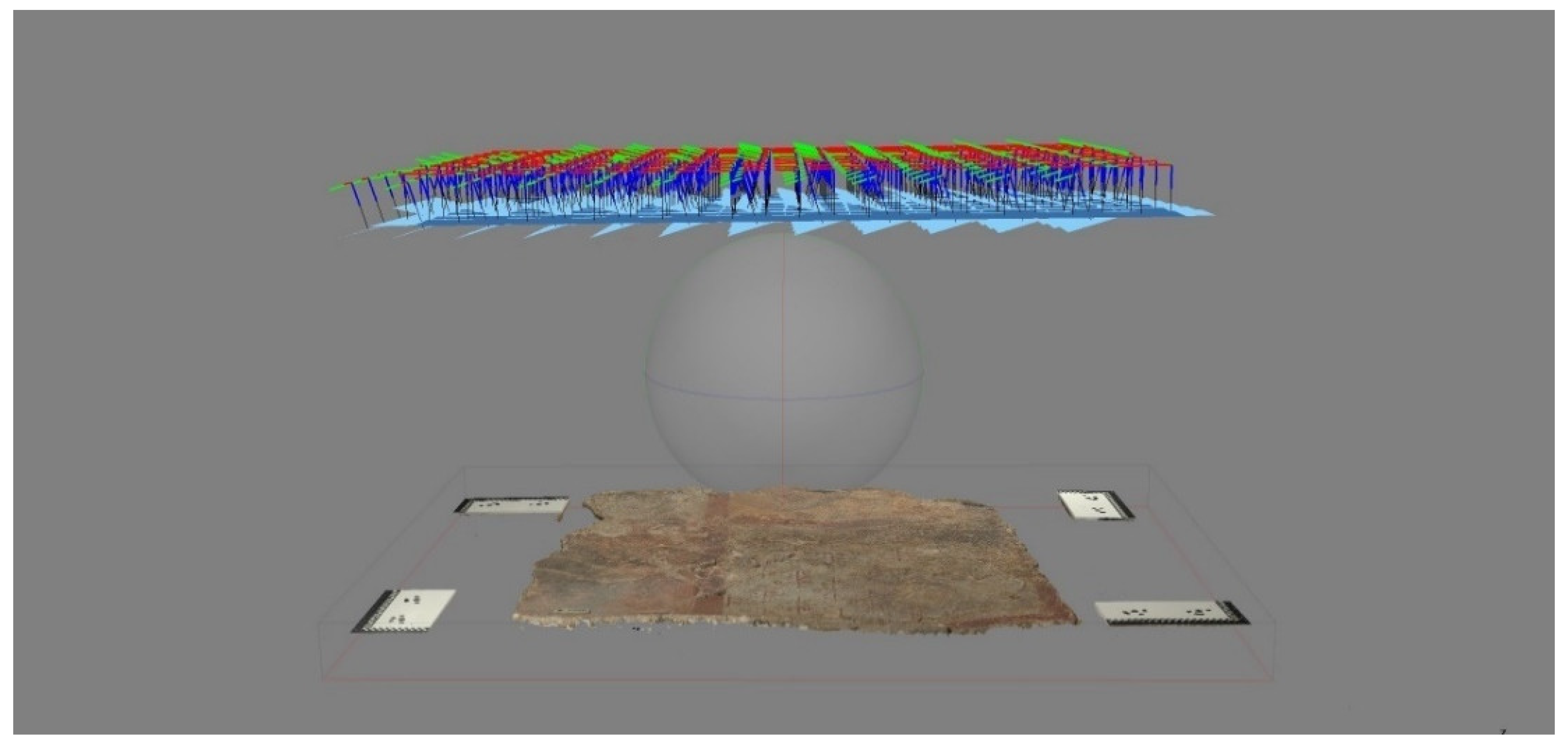
Figure 3.
Moreover, 49 images were acquired at a larger angle around the mural.
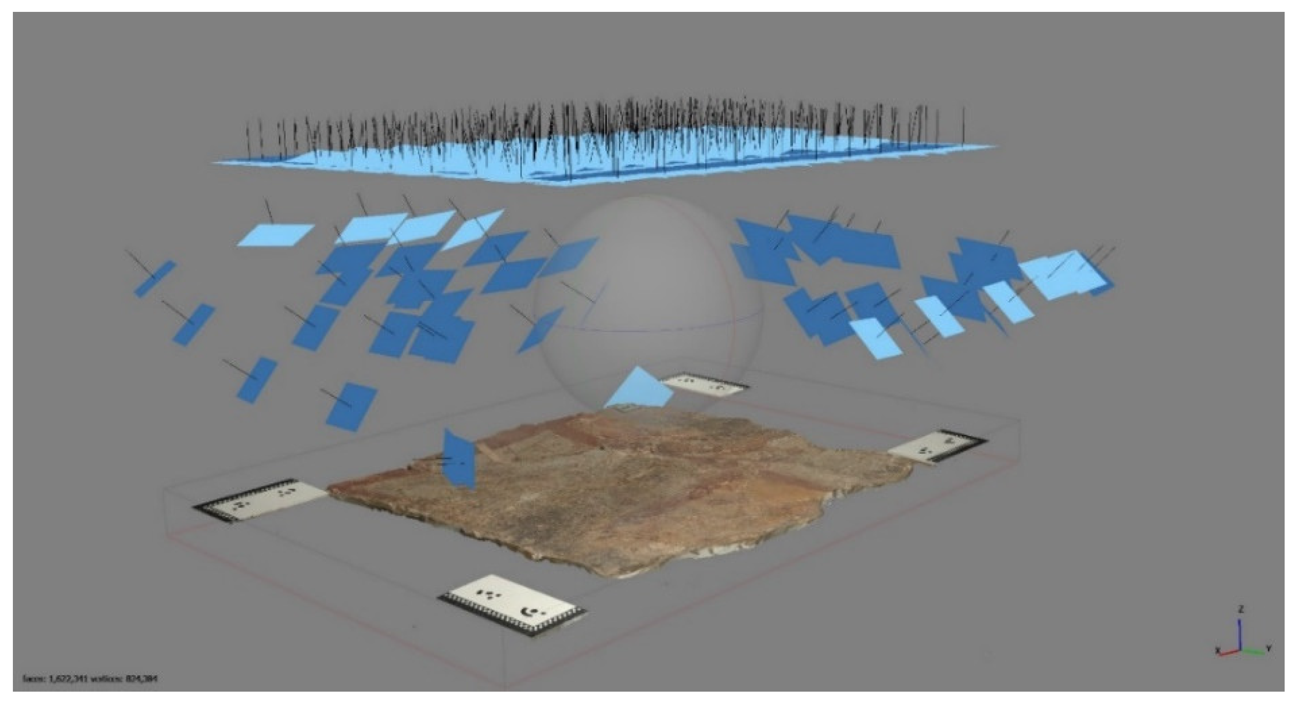
Figure 4.
The rotation angles (φ, ω, κ) of the camera’s tilt. The movement of the camera was according to the horizontal pane constituted by x and y coordinates.
Figure 4.
The rotation angles (φ, ω, κ) of the camera’s tilt. The movement of the camera was according to the horizontal pane constituted by x and y coordinates.
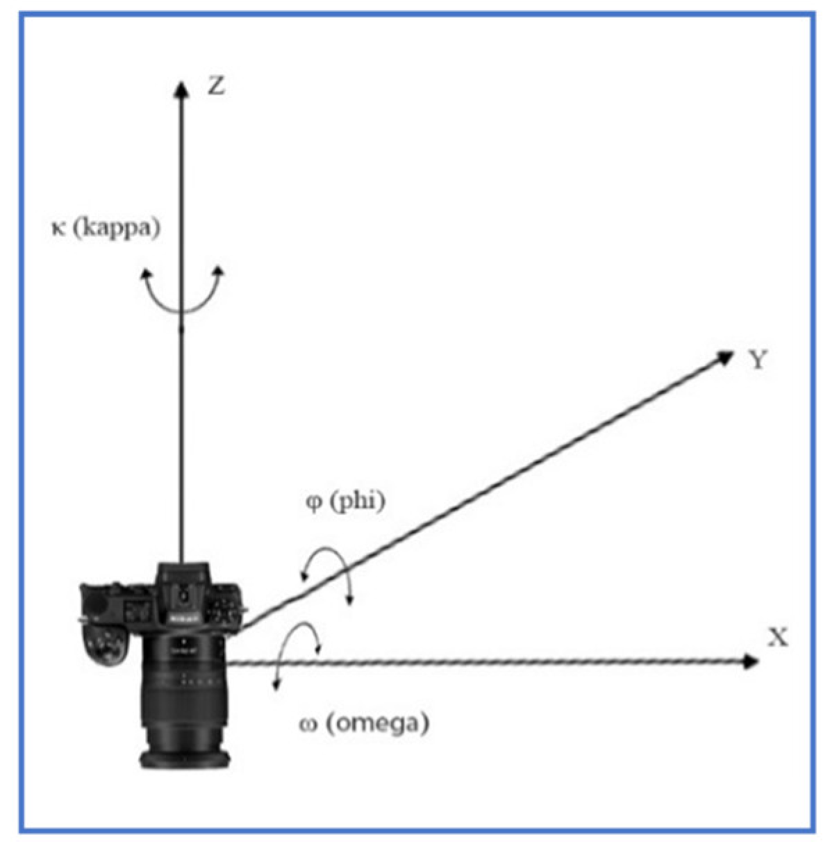
Figure 5.
The black dots indicate the positions of the camera, while the different colours represent the number of the overlapping images. The black outline delineates the surface of the mural. More overlap results in greater accuracy in the estimated measurements.
Figure 5.
The black dots indicate the positions of the camera, while the different colours represent the number of the overlapping images. The black outline delineates the surface of the mural. More overlap results in greater accuracy in the estimated measurements.
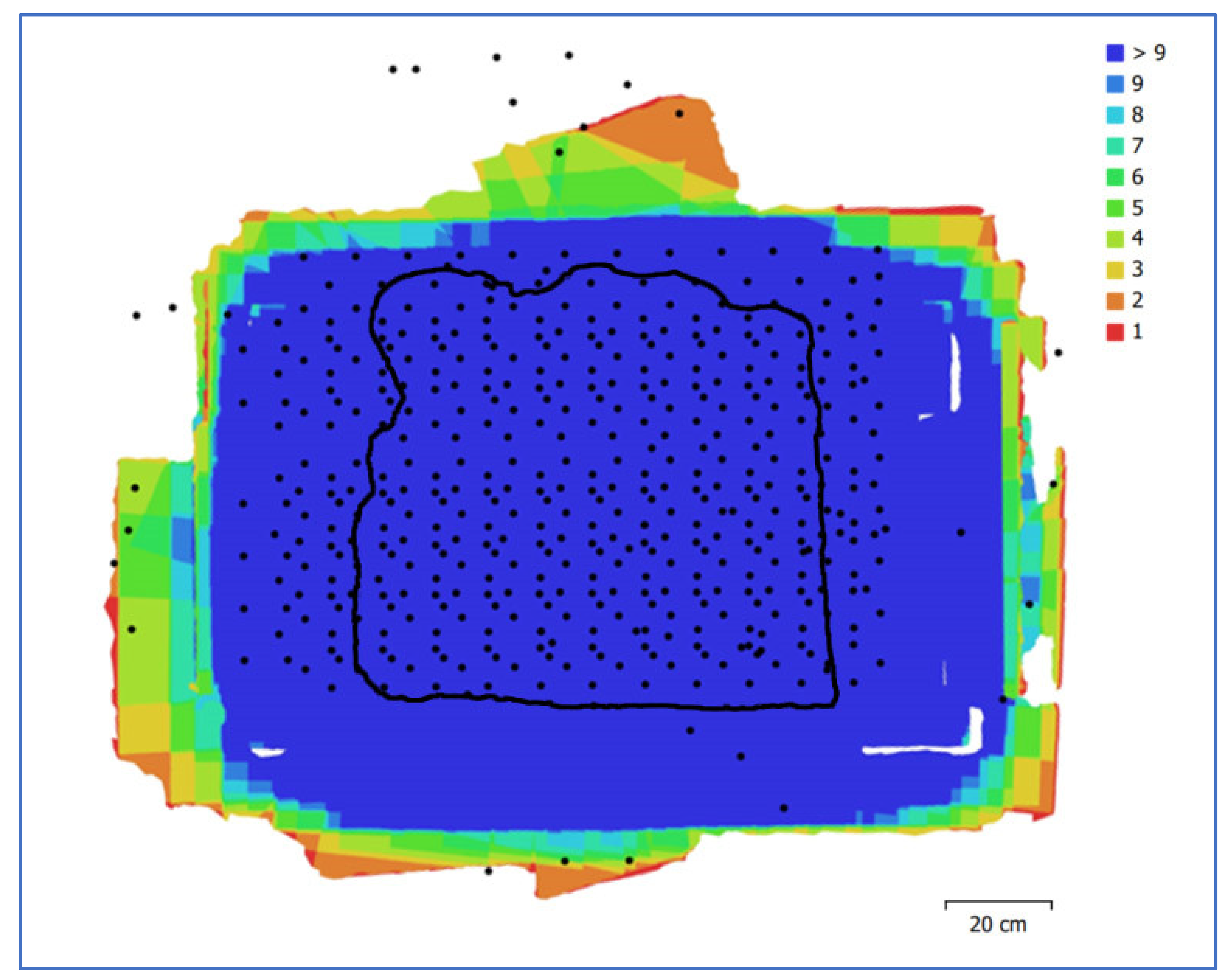
Figure 6.
8 coded targets (calibrated Agisoft’s markers) were placed on the surface of the mural. Outside the mural, 4 custom-made scale bars consisted of 90o angle rulers and 4 prefabricated coded pears of Metashape targets (1-8) with known highly accurate pre-measured distances in between located in such a way that the rulers on each side should form a straight line and be levelled at a plane consisting of the coded targets (5, 1, 7) and the painted surface.
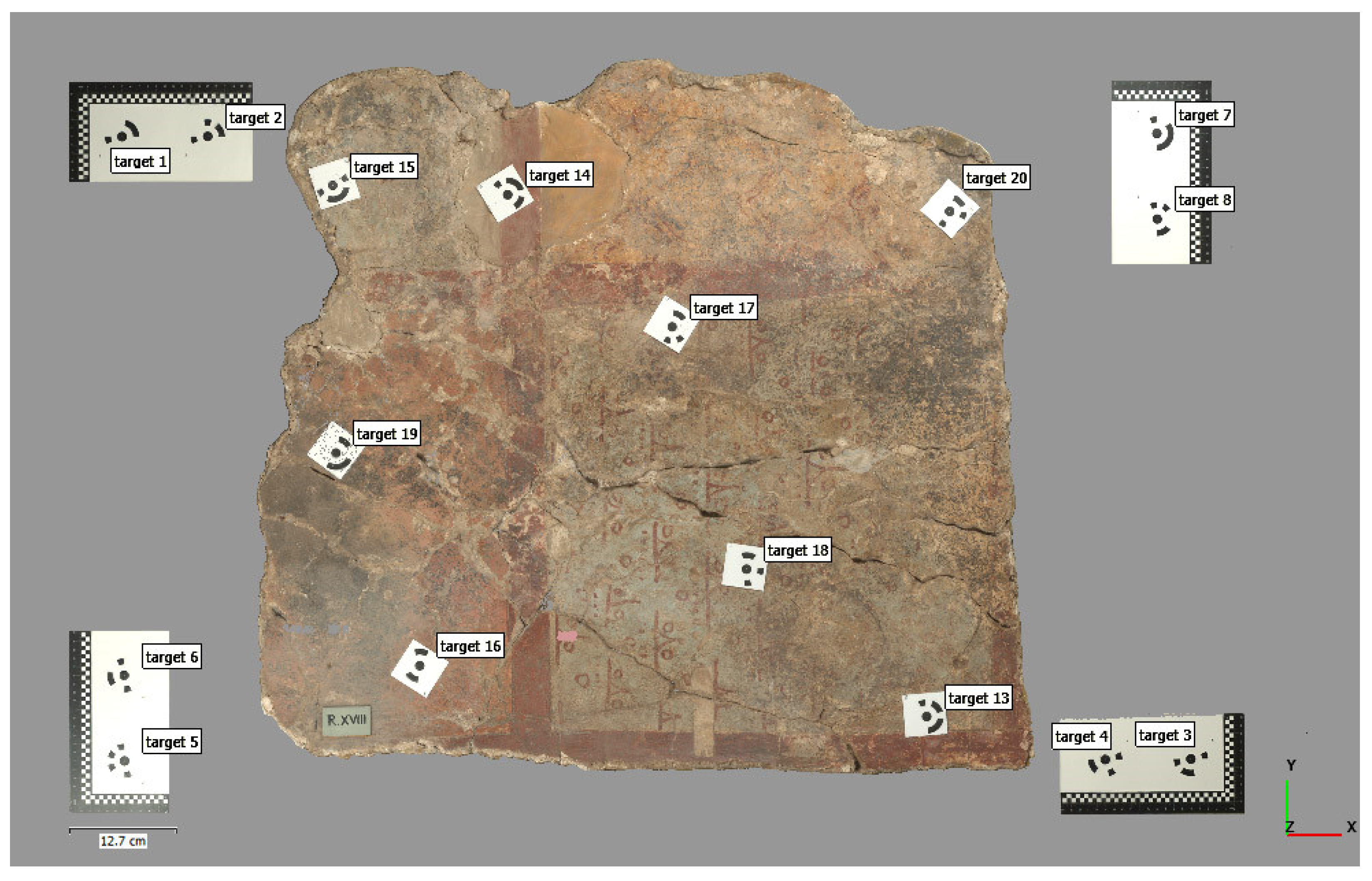
Figure 7.
A Line laser projects the laser beam as a line in order to position the rulers on each side of the mural forming a straight line.
Figure 7.
A Line laser projects the laser beam as a line in order to position the rulers on each side of the mural forming a straight line.
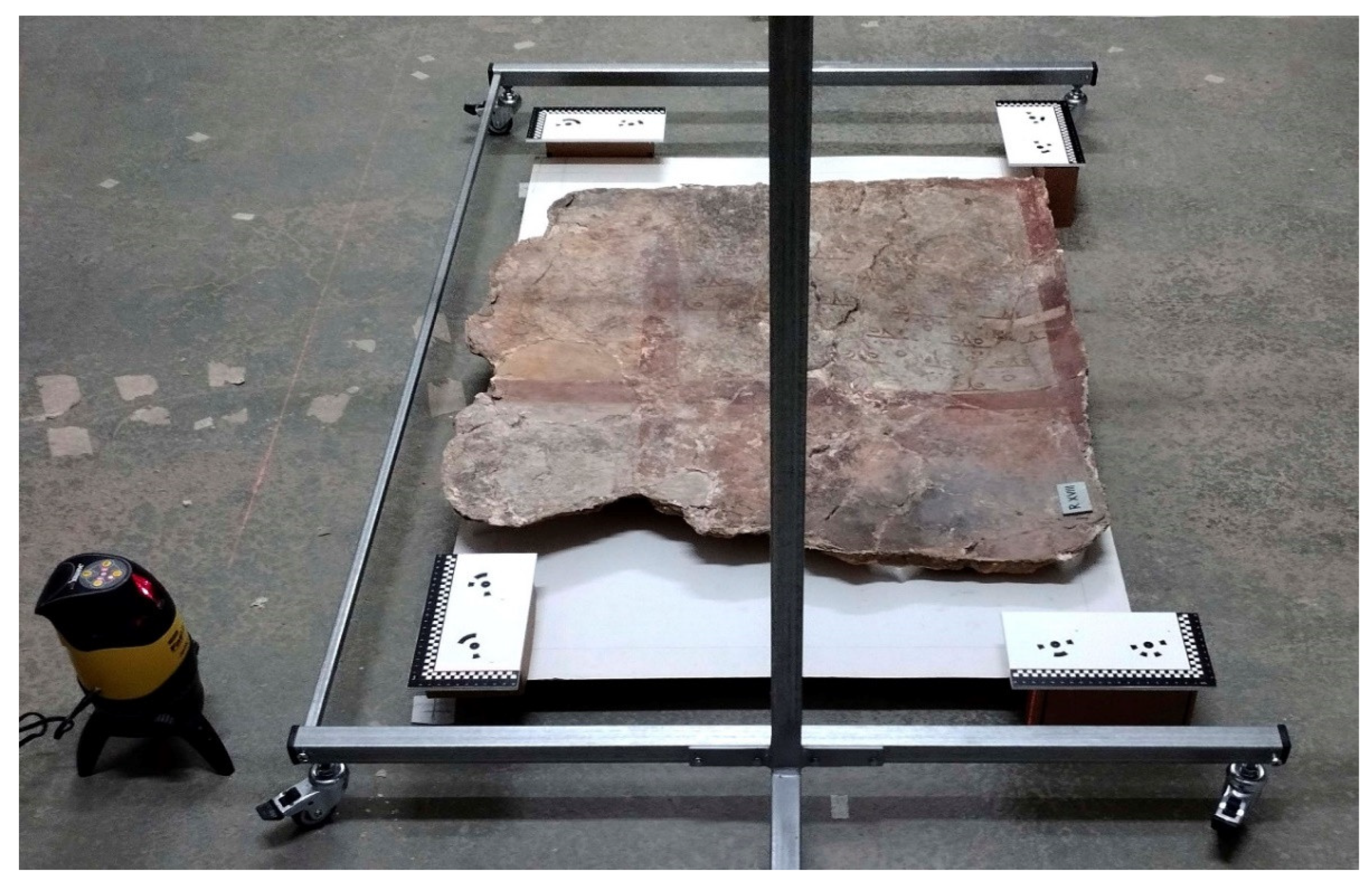
Figure 8.
The generated dense point cloud of the mural in the Agisoft Metashape environment.
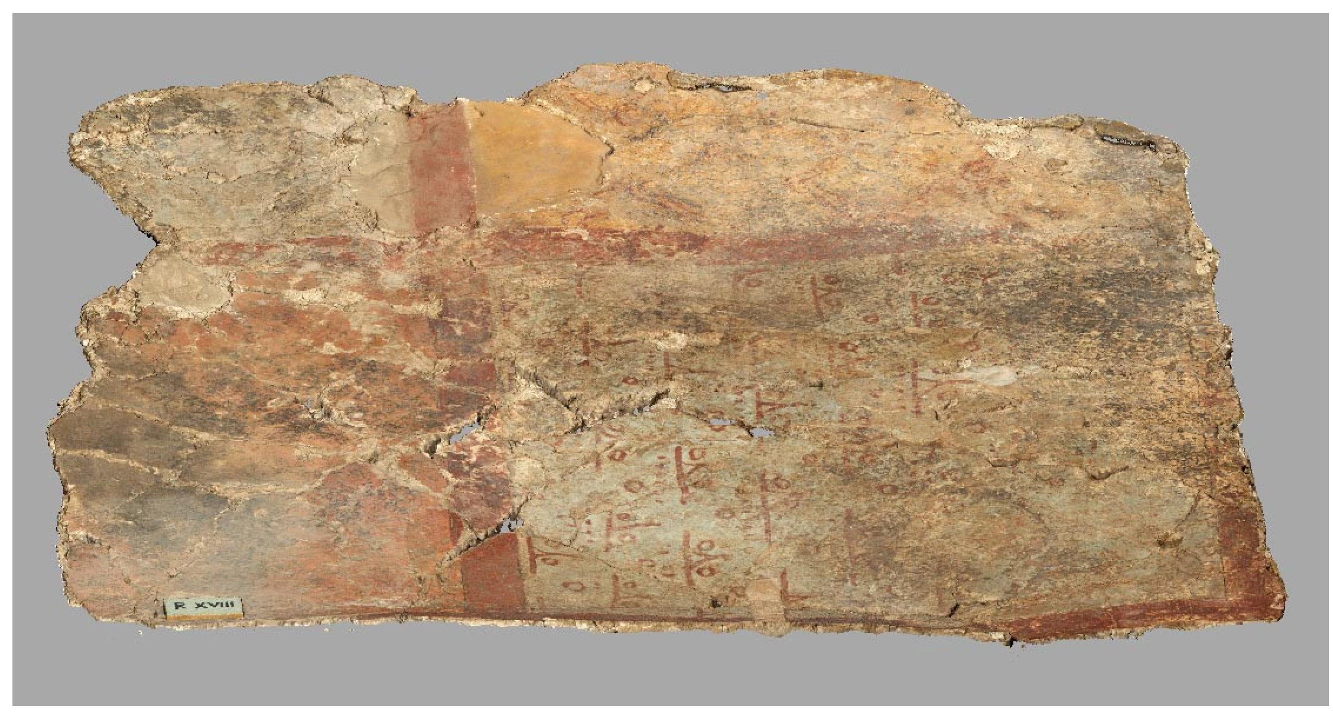
Figure 9.
The generated dense point cloud of the mural without texture.
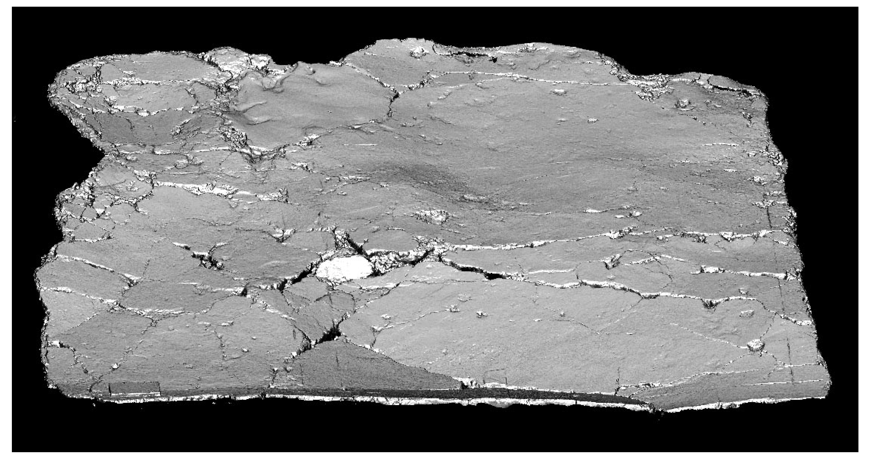
Figure 10.
a, b, c.: From top to bottom: a. wireframe (triangulated mesh) of the surface, b. 2.5D solid without texture and c. 2.5D model with texture. d, e, f.: Detail of Figure 10. a, b, c.
Figure 10.
a, b, c.: From top to bottom: a. wireframe (triangulated mesh) of the surface, b. 2.5D solid without texture and c. 2.5D model with texture. d, e, f.: Detail of Figure 10. a, b, c.
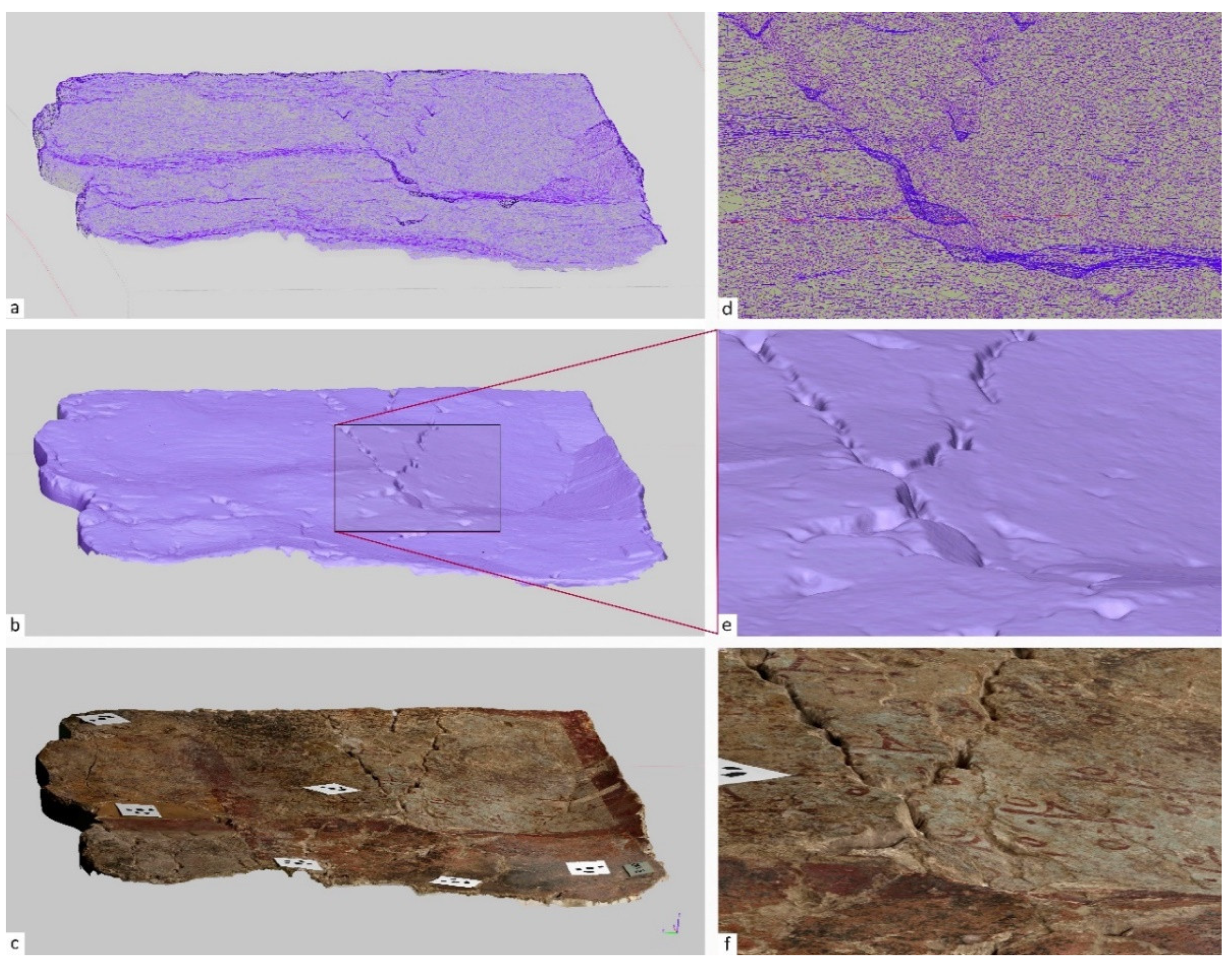
Figure 11.
The Dense Point Cloud of the area of Figure 10. d, e, f.
Figure 11.
The Dense Point Cloud of the area of Figure 10. d, e, f.
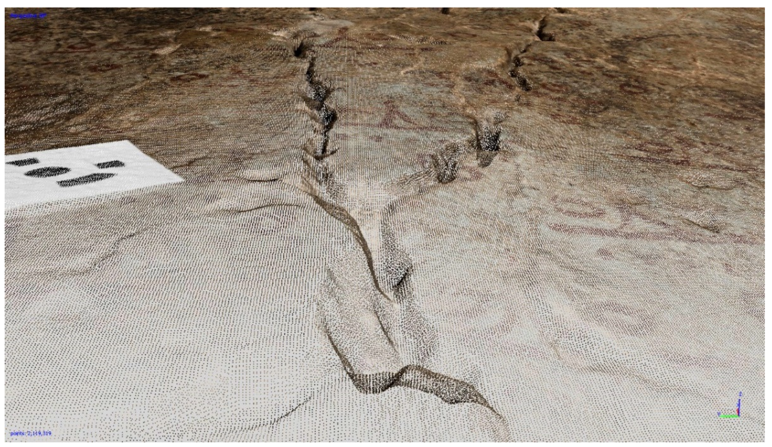
Figure 12.
The produced Dense Elevation Model (DEM) uses pixel locations to represent X and Y coordinates, and pixel values to represent the depth. The colour gradient corresponds to measurable altitudinal gradients. They can also be visualized in the form of elevation contours.
Figure 12.
The produced Dense Elevation Model (DEM) uses pixel locations to represent X and Y coordinates, and pixel values to represent the depth. The colour gradient corresponds to measurable altitudinal gradients. They can also be visualized in the form of elevation contours.

Figure 13.
The altitude differences can also be visualized in the form of contours. The generated contours have an interval of 0.001m.
Figure 13.
The altitude differences can also be visualized in the form of contours. The generated contours have an interval of 0.001m.
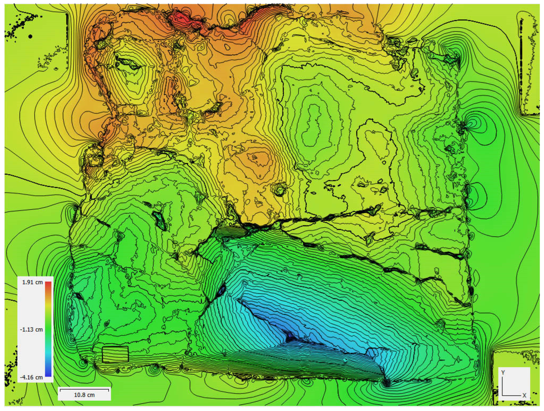
Figure 14.
Cross section with visual and metrical information about the relief and topography of the mural painting.
Figure 14.
Cross section with visual and metrical information about the relief and topography of the mural painting.
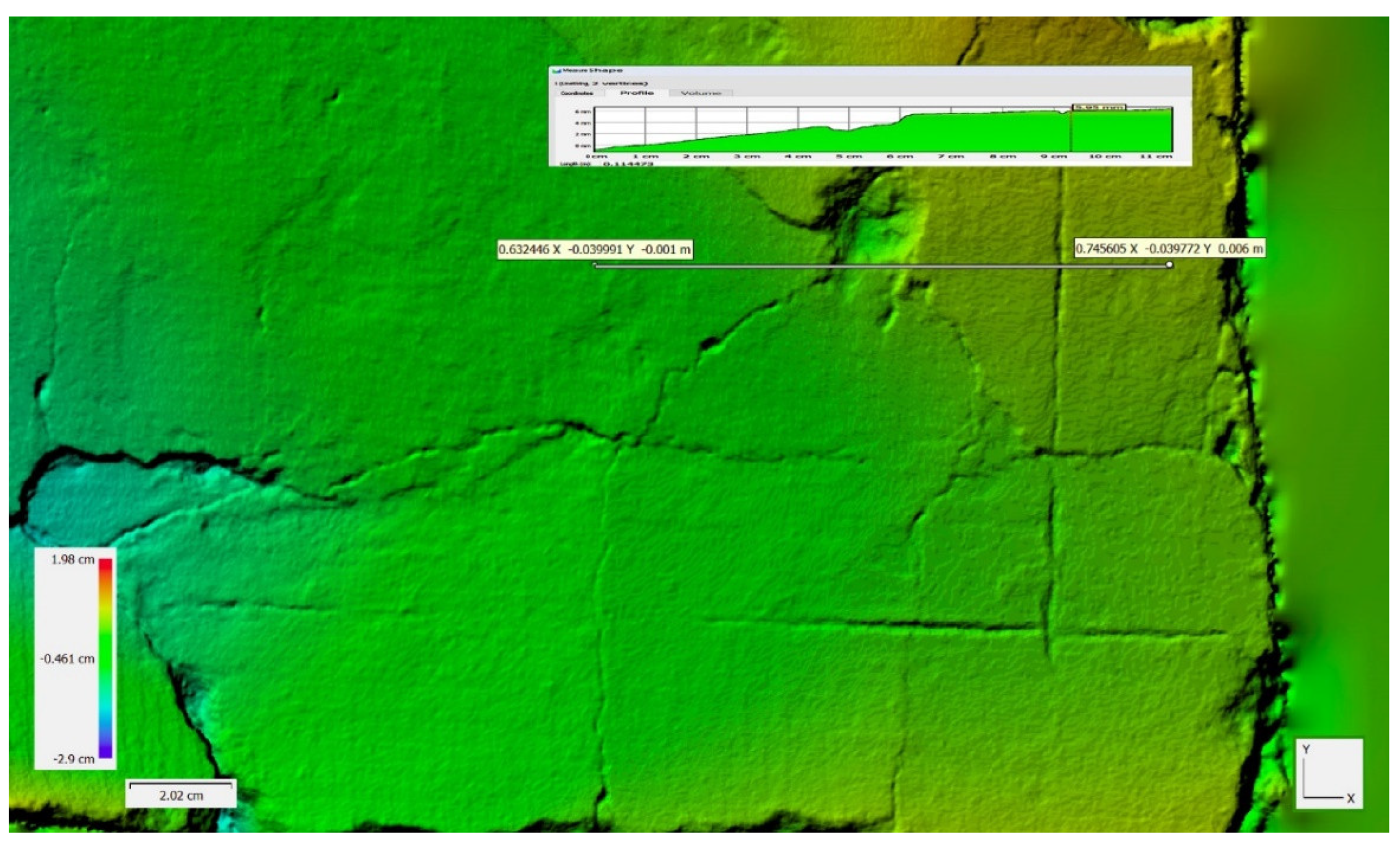
Figure 15.
The product of digital photogrammetry offers wealthy and valuable information concerning the object where the need to exploit it may arise at a later occasion. Having collected the data in a relatively inexpensive and quick process a plethora of information for now or in the future is available.
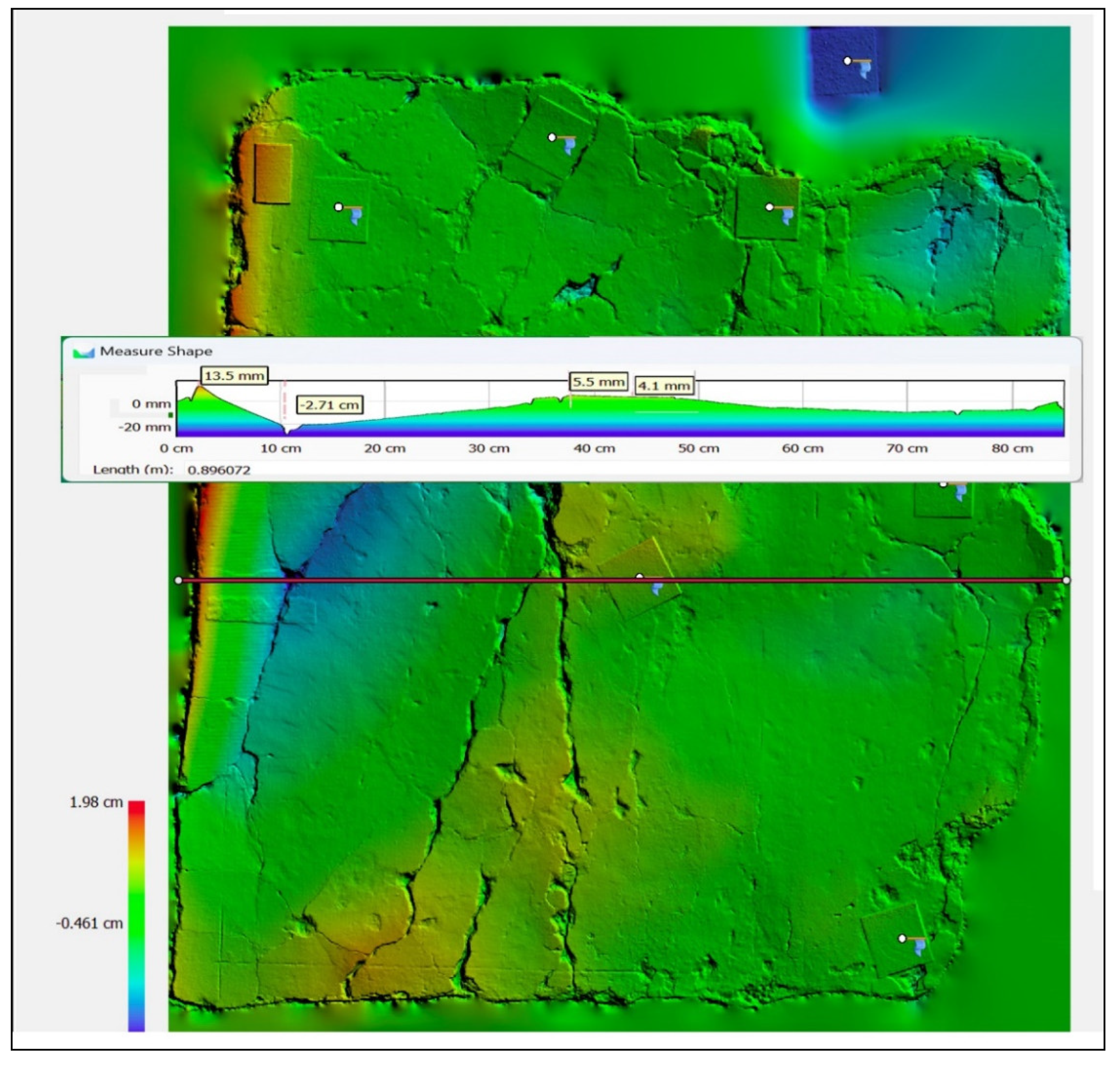
Figure 16.
The reconstructed orthomosaic from 89 DNG images with a total resolution of 26210x17852 pix, 0.0555mm/pix. It is ortho-projected on a plain defined by the three targets 5, 1, and 7 (Figure 6) which have z=0 on the local coordinate system.
Figure 16.
The reconstructed orthomosaic from 89 DNG images with a total resolution of 26210x17852 pix, 0.0555mm/pix. It is ortho-projected on a plain defined by the three targets 5, 1, and 7 (Figure 6) which have z=0 on the local coordinate system.
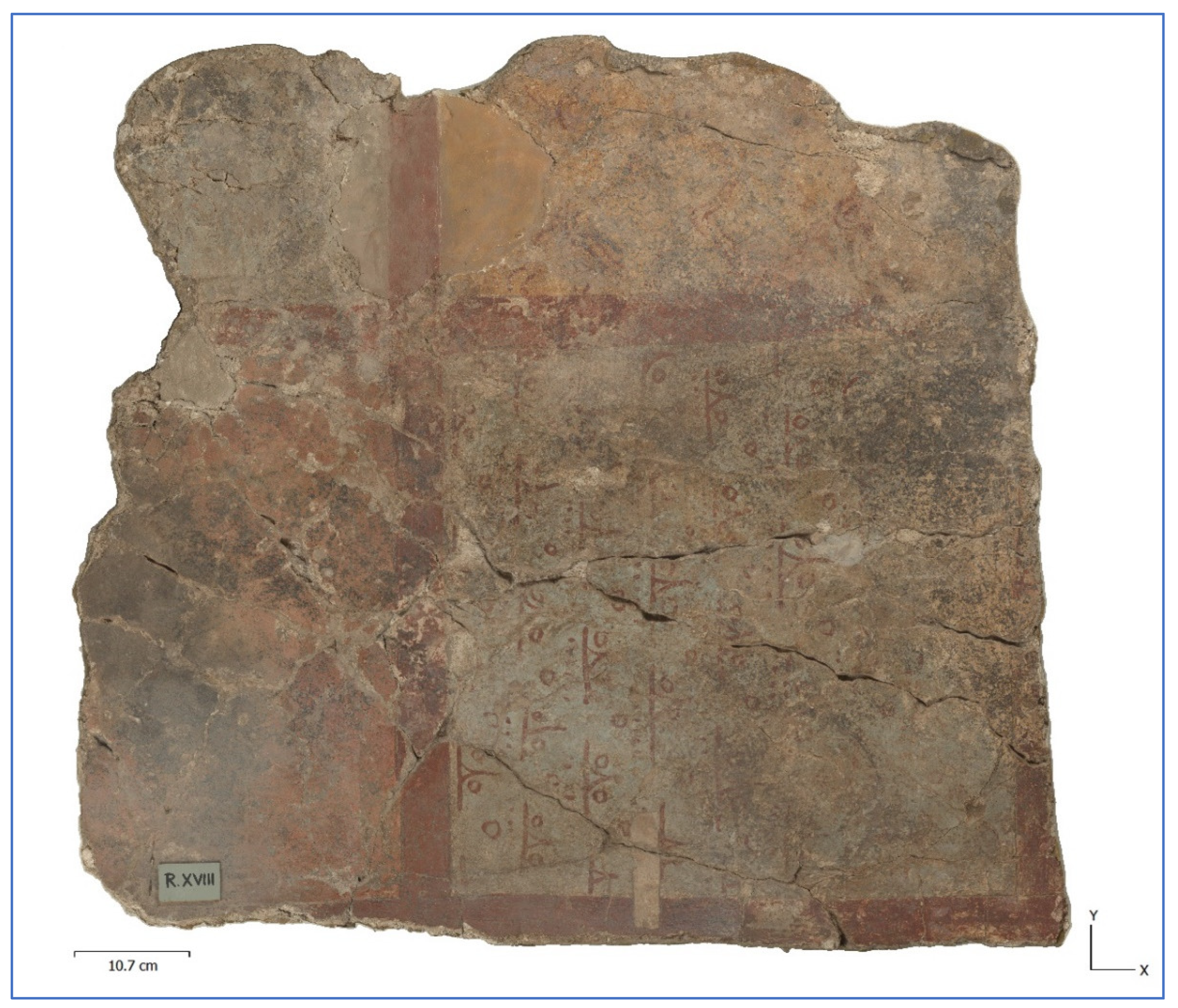
Figure 17.
Accurate measures on the reconstructed orthomosaic.
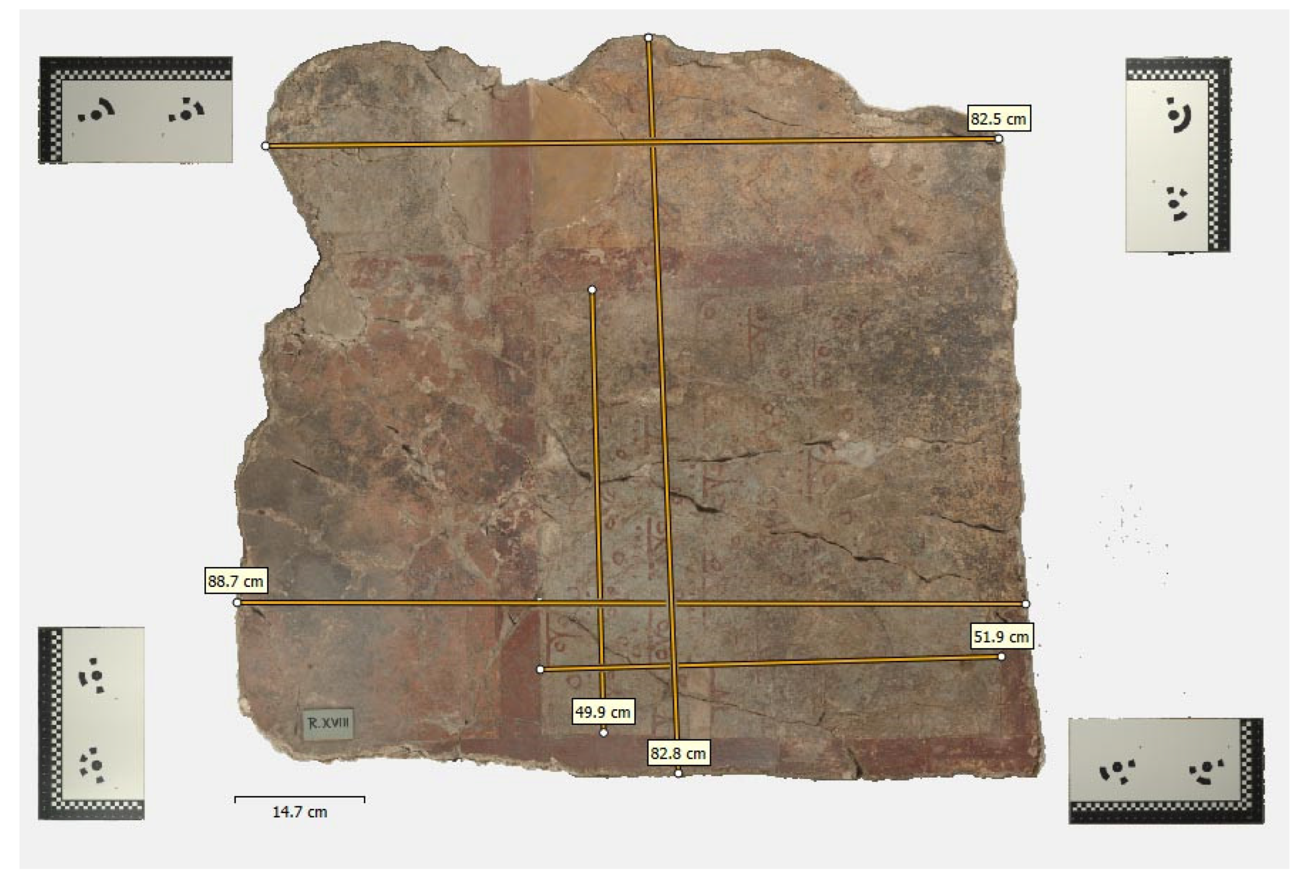
Figure 18.
Detail. Measures on the reconstructed orthomosaic.
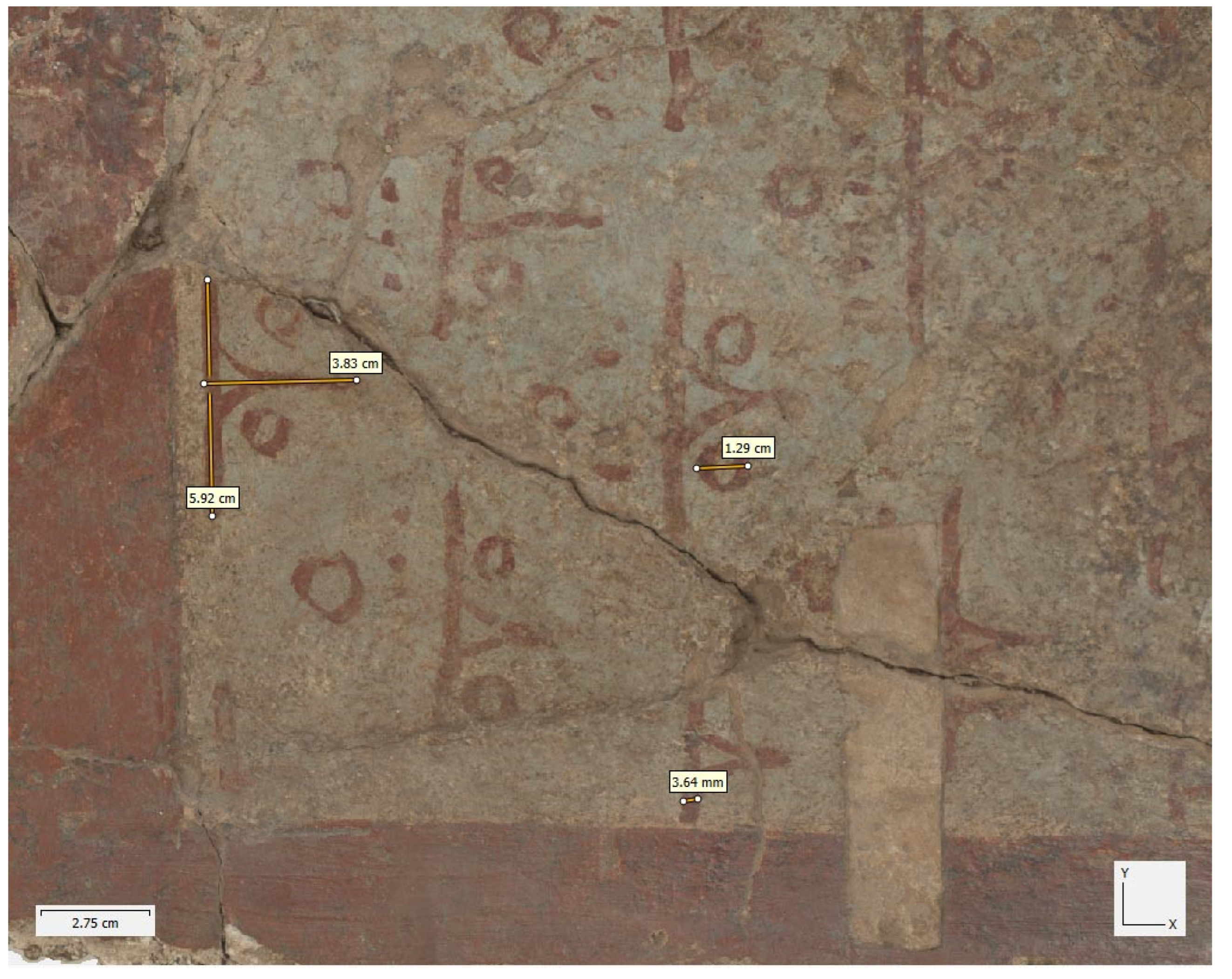
Figure 19.
Various precise measurements can be obtained on the wall painting not in situ, nor on the physical object, but at any office, in any place, at any time.
Figure 19.
Various precise measurements can be obtained on the wall painting not in situ, nor on the physical object, but at any office, in any place, at any time.
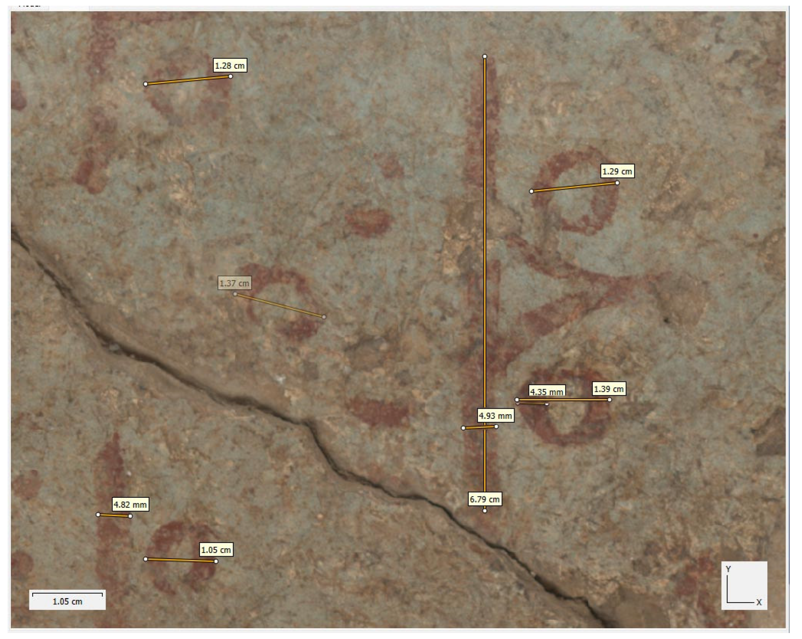
Figure 20.
RTIViewer screenshot. RTI reveals detailed surface texture, including brushstrokes and other subtle features that contribute to the artist’s technique. This allows for a more in depth understanding of the painting style and the artist’s skill.
Figure 20.
RTIViewer screenshot. RTI reveals detailed surface texture, including brushstrokes and other subtle features that contribute to the artist’s technique. This allows for a more in depth understanding of the painting style and the artist’s skill.
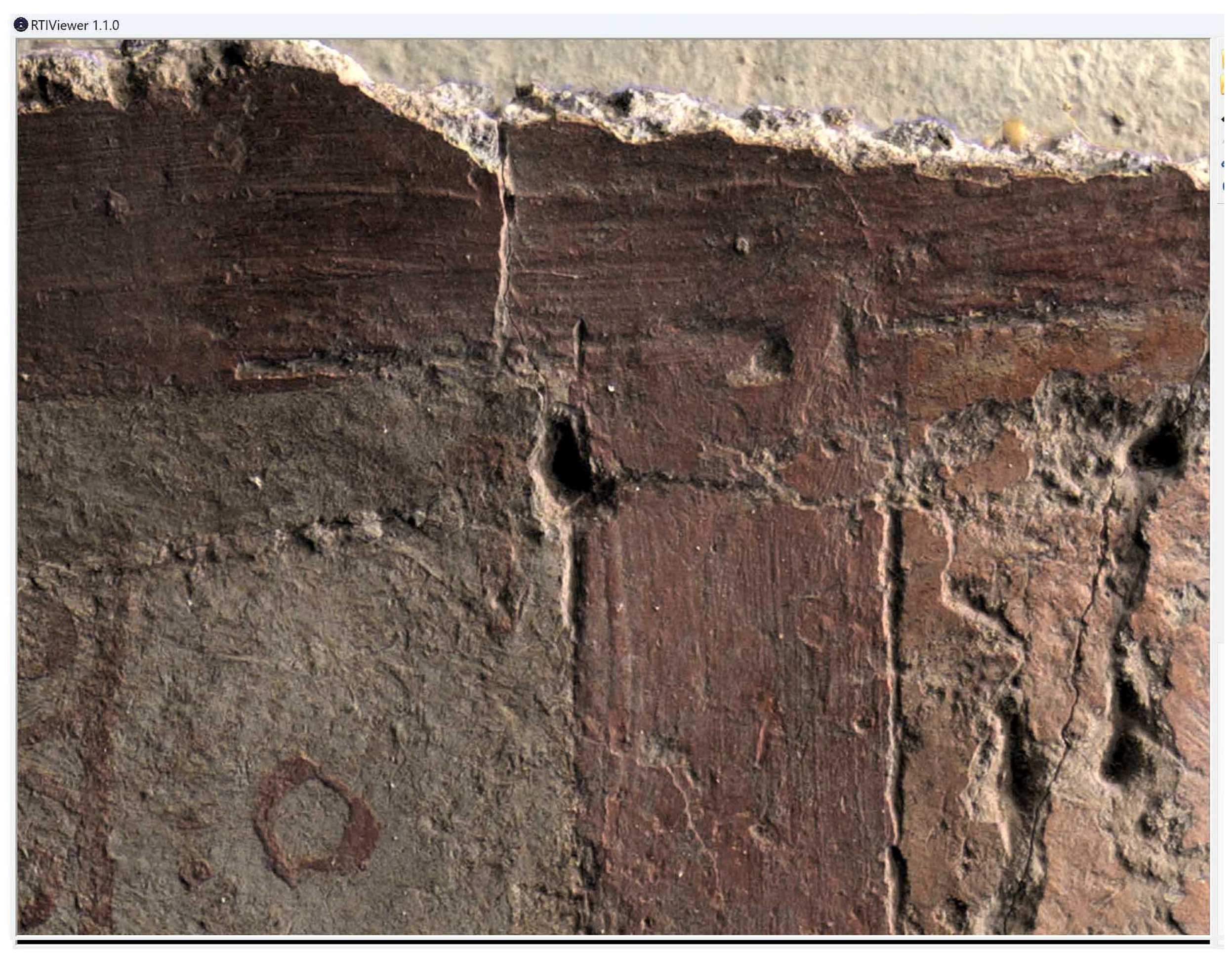

Table 1.
Summarized technical report of the procedure.
 |
Disclaimer/Publisher’s Note: The statements, opinions and data contained in all publications are solely those of the individual author(s) and contributor(s) and not of MDPI and/or the editor(s). MDPI and/or the editor(s) disclaim responsibility for any injury to people or property resulting from any ideas, methods, instructions or products referred to in the content. |
© 2024 by the authors. Licensee MDPI, Basel, Switzerland. This article is an open access article distributed under the terms and conditions of the Creative Commons Attribution (CC BY) license (http://creativecommons.org/licenses/by/4.0/).
Copyright: This open access article is published under a Creative Commons CC BY 4.0 license, which permit the free download, distribution, and reuse, provided that the author and preprint are cited in any reuse.


