
Submitted:
27 May 2025
Posted:
28 May 2025
You are already at the latest version
Abstract
This study evaluates three advanced approaches for 3D reconstruction of challenging transparent surfaces: conventional photogrammetry, enhanced 3D Gaussian Splatting, and novel 2D Gaussian Splatting (2DGS). Through a detailed case study of a glass artifact, the research demonstrates 2DGS's superior performance in geometric reconstruction and multi-view consistency, leveraging its innovative planar representation to outperform alternative methods in capturing fine surface details and complex internal structures. While the enhanced 3D approach shows advantages in visual rendering quality, it exhibits surface artifacts, and traditional photogrammetry proves inadequate for complete reconstruction. The comparative analysis highlights 2DGS's balanced capabilities in structural accuracy and perceptual quality, albeit with higher computational demands. These findings establish 2DGS as a significant advancement for cultural heritage documentation, particularly for transparent and reflective objects requiring precise digital preservation. The study identifies key directions for future development, including performance optimization and accessibility improvements, to facilitate broader adoption in heritage conservation and remote sensing applications where accurate 3D documentation is essential.
Keywords:
3D Gaussian Splatting
; SuGaR
; 2D Gaussian Splatting
; 3D mesh reconstruction
; MLP
; Deep Learning
; Machine learning
; NeRFs
1. Introduction
The reconstruction of three-dimensional geometries from input data is a fundamental challenge in remote sensing and related fields. This process is often both time-intensive and complex, particularly when dealing with existing structures and the intricate nature of building stocks. These challenges are further exacerbated in the context of Cultural Heritage (CH), where structures are often characterized by irregular geometries, heterogeneous materials, and unique aesthetic and historical values [1]. Reconstructing such geometries requires a high level of accuracy to ensure both the metric and visual fidelity of the 3D models.
Photogrammetric approaches, such as Structure-from-Motion and Multi-View Stereo (SfM-MVS), are frequently employed for 3D reconstruction [2]. However, these methods often fall short in capturing critical surface details, especially in cases involving reflective or transparent materials [3,4], homogeneous textures, or non-Lambertian surfaces. These shortcomings highlight the limitations of conventional techniques when applied to complex artefacts or scenes, such as those commonly found in CH preservation.
Recent advances in technology, particularly the integration of Computer Vision (CV) and Artificial Intelligence (AI) into photogrammetry, have opened up new possibilities for overcoming these challenges. Emerging methodologies, including Neural Radiance Fields and 3D Gaussian-Splatting, offer promising pathways for enhancing the accuracy and efficiency of 3D reconstructions. These techniques aim to address the limitations of traditional methods by leveraging data-driven models that adapt to complex and variable surface properties.
This study explores these cutting-edge approaches, presenting a novel workflow that incorporates CV and AI advancements into photogrammetric workflows. A comparative evaluation of both quantitative (metric) and qualitative (visual) outcomes underscores the potential of these innovations for improving 3D modeling practices, particularly for CH applications.
2. State of Art
The field of 3D reconstruction has undergone significant transformation with the advent of AI and CV techniques [5,6,7]. SfM-MVS, have served as the cornerstone for creating 3D models from overlapping images. While these methods are highly effective for many applications, their limitations in handling complex materials and geometries have been well-documented. For instance, reflective, transparent, or homogeneous surfaces often lead to data gaps or inaccuracies in standard workflows.
In recent years, researchers have increasingly turned to advanced algorithms and machine learning models to address these challenges. Neural Radiance Fields (NeRFs) [8,9] have emerged as a promising technology for photorealistic 3D reconstruction, particularly for scenes with intricate lighting and material interactions [10]. NeRFs model the radiance emitted from a 3D scene using deep neural networks, allowing for the synthesis of novel views while maintaining high fidelity in surface representation.
Similarly, 3DGS [11] has gained attention for its ability to efficiently approximate complex surface geometries using a probabilistic framework. By representing surfaces as a collection of Gaussian splats, this method reduces computational overhead while maintaining accuracy in rendering, making it suitable for real-time applications.
2DGS [12] is introduced to address the limitations of 3DGS in accurately representing thin surfaces due to multi-view inconsistencies.
These advancements reflect a broader trend towards hybrid methodologies that combine SfM-MVS with AI-driven solutions. Such approaches not only improve the metric accuracy of reconstructions but also enhance their visual realism, offering significant benefits for applications in CH and beyond. The integration of these techniques is paving the way for a new era of 3D modeling, where complex artefacts and challenging scenes can be accurately reconstructed with unprecedented detail and efficiency.
2.1. Gaussian-Splatting and Evaluation Metrics
The workflow (Figure 1) commences with SfM process, which reconstructs camera poses from unordered images while producing sparse 3D point clouds of the scene. The input 3DGS consists of static images, calibrated using the camera poses from SfM, along with the sparse point clouds.
From these 3D points, a set of anisotropic Gaussian ellipsoids is generated, with each ellipsoid represented by a 3D Gaussian distribution. These ellipsoids are then projected onto 2D images from various viewpoints, using the recovered camera pose information. The differentiable Gaussian functions within the camera frustum are rendered into images through rasterization. Next, a loss function is computed by comparing the rendered images to the ground truth images, and the parameters of each Gaussian distribution (such as position, size, and orientation) are adjusted accordingly. An adaptive density control method is also applied to optimize the properties of the Gaussian ellipsoids, including their position, size, orientation, quantity, color, and opacity in the scene.
In standard settings for novel view synthesis using 3DGS, visual quality assessment metrics are used for benchmarking. The most widely adopted metrics in the literature include Peak Signal-to-Noise Ratio (PSNR), Structural Similarity Index Measure (SSIM) [14], and Learned Perceptual Image Patch Similarity (LPIPS) [15].
PSNR is used to compare the similarity between rendered images generated by models and real images. A higher PSNR value indicates greater similarity and better image quality. However, PSNR has some limitations as it primarily focuses on mean square error, overlooking human eye sensitivity to different frequency components and the effects of perceptual distortions. As a result, PSNR may not always accurately reflect the perceived differences in image quality from a human perspective.
SSIM is a metric for measuring the structural similarity between two images, taking into account brightness, contrast, and structure. SSIM values range from −1 to 1, with values closer to 1 indicating higher similarity between the two images.
LPIPS evaluates the similarity between two images based on feature representations extracted from a pre-trained deep neural network. The original LPIPS paper used SqueezeNet [16], VGG [17], and AlexNet [18] as feature extraction backbones. LPIPS scores are more closely aligned with human perceptual judgments compared to traditional metrics like PSNR and SSIM. A lower LPIPS score indicates higher similarity between the images.
Unlike traditional metrics such as PSNR and SSIM, which calculate differences based on raw pixel values or simple transformations thereof, LPIPS leverages deep learning to better align with human visual perception. It uses the distance between features extracted by a convolutional neural network (CNN) pretrained on an image classification task as a perceptual metric.
In Table 1 are shown the metric quality thresholds:
2.2. Optimizations from the Original Paper of 3DGS
The Gaussian Splatting technique represents a particularly promising direction for 3D reconstruction, as evidenced by the growing interest within the scientific community and the increasing number of publications dedicated to the subject. Numerous recent studies focus on improving this methodology, addressing aspects such as computational efficiency, rendering quality, the handling of thin structures, and multi-view consistency. Among the most significant contributions are the following:
2.2.1. Storage Reduction
Several storage reduction strategies are employed in 3DGS. The number of 3D Gaussian primitives is reduced through masking in Compact-3DGS [19] and HAC [20], while pruning methods in LightGaussian [21], EAGLES [22], and reduced-3DGS [23] minimize Gaussian count. View-dependent color optimization is achieved by replacing spherical harmonics with grid-based neural fields in Compact-3DGS and adjusting spherical harmonic bands in reduced-3DGS. Additionally, quantization and compression techniques further optimize storage.
To enhance 3D Gaussian model densification and accuracy, techniques like geometric priors and integration with 2D depth and normal maps are used to refine Gaussian placement and orientation. Frequency-based regularization methods help control over-reconstruction, reducing artifacts like blurring and ghosting. More uniform and surface-aligned Gaussian splitting methods improve precision, which is critical for point cloud extraction and editing tasks.
Key improvements focus on frequency control, with methods like Mip-Splatting minimizing aliasing artifacts. Multi-scale adaptation ensures Gaussian primitives dynamically adjust to resolution changes, maintaining rendering quality. Other improvements include adjusting color and opacity based on viewpoint changes, implementing simplified shading functions for reflective surfaces, and developing hybrid models like VDGS [24], which combine 3DGS with neural network-based encoding for accurate, view-dependent color and opacity updates.
2.2.2. Surface Mesh Extraction
It is a crucial task in computer graphics and CV, aimed at generating a 3D mesh from various representations of objects or scenes. Mesh-based representations are essential for editing, sculpting, animating, and relighting. However, extracting a mesh from the 3D Gaussian Splatting (3DGS) representation, which uses Gaussian distributions, presents significant challenges due to the lack of inherent structure in the Gaussians. SuGaR [25] introduces a novel regularization term that aligns Gaussians with the scene's surface, enabling mesh extraction via Poisson reconstruction. This method is fast, scalable, and preserves detail, unlike the Marching Cubes algorithm [43], typically used for mesh extraction from Neural SDFs. SuGaR also offers an optional refinement strategy that binds Gaussians to the mesh surface, jointly optimizing both the Gaussians and the mesh through Gaussian splatting rendering.
GS2Mesh: Gaussian Splatting-to-Mesh [26] bridges the gap between noisy 3DGS and a smooth 3D mesh by incorporating real-world knowledge into the depth extraction process. Instead of directly extracting geometry from Gaussian properties, GS2Mesh uses a pre-trained stereo-matching model to guide the process. It renders stereo-aligned image pairs, feeds them into a stereo model to obtain depth profiles, and fuses these profiles into a single mesh. This approach results in smoother, more accurate reconstructions with finer details compared to other surface reconstruction methods, with minimal overhead on top of the 3DGS optimization process.
GOF: Gaussian Opacity Fields [27] proposes an efficient and high-quality method for surface reconstruction in unbounded scenes. Building on ray-tracing-based volume rendering of 3D Gaussians, GOF directly extracts geometry by identifying the level set of Gaussians, bypassing Poisson reconstruction or TSDF fusion. It approximates surface normals through the ray-Gaussian intersection plane and applies regularization to improve geometry accuracy. Additionally, GOF introduces an efficient geometry extraction technique using marching tetrahedra, adapting to scene complexity.
2DGS: 2D Gaussian-Splatting [12] introduces a novel approach by collapsing 3D volumes into 2D oriented planar Gaussian disks. Unlike 3D Gaussians, 2D Gaussians model surfaces consistently from different views. 2DGS employs a perspective-accurate splatting process with ray-splat intersections and rasterization to recover thin surfaces accurately. It also integrates depth distortion and normal consistency terms to enhance reconstruction quality.
2DGS simplifies the 3D volume by representing it as a collection of 2D oriented planar Gaussian disks [32], which ensure view-consistent geometry. To improve the quality of reconstructions, two regularization terms are introduced: depth distortion and normal consistency. The depth distortion term focuses on concentrating the 2D primitives within a narrow range along the viewing ray, while the normal consistency term ensures that the rendered normal map aligns with the gradient of the rendered depth. This method guarantees precise surface representation, delivering state-of-the-art performance in both geometry reconstruction and novel view synthesis.
MVG-Splatting: Multi-View Guided Gaussian Splatting with Adaptive Quantile-Based Geometric Consistency Densification [28], It introduces a method that utilizes depth-normal mutual optimization to guide a more precise densification process, enhancing the detail representation for scene rendering and surface extraction. Building on the 2DGS framework [12], it implements a more robust technique for recalculating surface normals. These recalculated normals, combined with gradients from the original images, help refine the accuracy of the rendered depth maps. It then proposes an efficient multi-level densification approach based on multi-view geometric consistency [29], which directs the refined depth maps to accurately project onto under-reconstructed regions. In contrast to previous GS-based geometric reconstruction methods [30,31,32,33], its approach first generates high-quality, uniformly densified Gaussian point clouds. This allows for direct surface extraction using the Marching Cubes method [34] on the point cloud. Additionally, it adaptively determines voxel sizes for each densified Gaussian point cloud and uses multi-view normal maps to smooth and optimize surface normals, resulting in high-detail mesh surface extraction.
5. Materials
The dataset focuses on individual case studies representing critical challenges for photogrammetry in mesh model reconstruction, particularly when dealing with reflective surfaces, transparent materials, homogeneous textures, and non-Lambertian surfaces.
The pilot case study consists of a glass bottle (Mario Luca Giusti Transparent Bona Bottle) placed on a motorized turntable against a uniform neutral-gray background.
This controlled environment was specifically designed to optimize the AI-based masking process in Adobe Lightroom Classic (Figure 2), which proved essential for isolating the object of interest. By removing background interference through automated masking, all subsequent processing software could concentrate their analysis exclusively on the target object, significantly improving feature matching accuracy and reducing reconstruction artifacts.
To ensure the alignment of the various frames and to scale the 3D model, both single and double markers with scale bars are printed and located around the object.
For the purposes of creating a ground truth useful for comparing the data processing within the various software, an initial acquisition was made of the glass bottle entirely lined with a paper sticker (of negligible thickness), subsequently painted with artistic motifs to guarantee a complete and accurate photogrammetric model reconstruction.
To ensure model scalability and metric error control, the photogrammetric survey was supported by a high-precision topographic survey. During this topographic survey, the coordinates of 27 markers placed on the rotating platform were acquired using a total station Leica TCRP 1201, with an accuracy of up to one-tenth of a millimeter. The acquisition was carried out following rigorous protocols, ensuring that each marker was measured with extreme precision to guarantee accurate alignment and a reliable metric reconstruction of the 3D model.
The 227 images of the pilot dataset were acquired with a Nikon D750 camera with the characteristics shown in Table 2.
The image acquisition settings are shown in the Table 3.
Tests are conducted using an NVIDIA GeForce RTX 4090 GPU (24 GB VRAM) and an AMD Ryzen 97950X 16-Core CPU.
5.1. Software and Environment Employed
- Agisoft Metashape v.2.0.0
- Lightroom Classic v.14.0.1
- Cloud Compare v.2.13.2
- 3D Gaussian-Splatting (latest code update on Aug. 2024)
- SuGaR (latest code update on Sept. 2024)
- 2D Gaussian-Splatting (latest code update on Dec. 2024)
- Anaconda environment v.conda 23.7.4
6. Methodology
The methodology adopted in this study was designed to compare and integrate different 3D reconstruction technologies, starting from a common input and developing through three parallel processes that employ different software and approaches. The ultimate goal is to obtain a comparative evaluation of the results generated by each process, both quantitatively (through objective metrics) and qualitatively (through visual analysis).
6.1. Common Input and Initial Phase
The starting point of the methodology is represented by a common input, derived from the generation of a sparse point cloud. This initial phase is crucial, as it solves the photogrammetric problem by determining the internal and external parameters of the cameras used to capture the images. Traditionally, this operation is performed using the open-source software COLMAP, which is widely recognized for its effectiveness in 3D reconstruction based on SfM. Nonetheless, COLMAP struggled to align all the images correctly in our dataset, leading to incomplete reconstructions and inconsistencies in camera parameter estimation. In this work, we chose to use an executable script that leverages input data generated by the SfM analysis performed with Agisoft Metashape software.
This choice offers a dual advantage: it ensures a complete dataset alignment and a high-quality sparse point cloud, which serves as a common base for all three parallel processes.
The common parameters for the alignment are shown in Table 4:
The implemented workflow began with generating an initial sparse point cloud using the unmasked images with the automate detected markers, followed by a systematic path replacement operation employing the "Change Path" command to transition to the masked image set while meticulously preserving the established camera alignment parameters.
6.2. Parallel Reconstruction Processes
The methodology involves the use of three distinct approaches for 3D reconstruction, each based on different technologies and software (Figure 3):
6.2.1. Structure from Motion (SfM)
The first process is based on the SfM technique, which uses photogrammetric algorithms to reconstruct 3D geometry from 2D images. This approach is well-established and provides a solid basis for comparison with the other two more innovative methods. The parameters for generate the model are shown in Table 5:
6.2.2. 3D Gaussian Splatting (3DGS) + SuGaR
The 3DGS technique uses 3D Gaussians to represent the scene. A Gaussian in this context is a density distribution used to model the light and energy radiated from a point in space. However, 3DGS has limitations: 3D Gaussians fail to accurately represent object surfaces (e.g., thin surfaces like edges) due to "multi-view inconsistency." In other words, surfaces may appear distorted or imprecise from different angles.
To address this issue, SuGaR has been introduced as an extension of 3DGS, aiming to improve the reconstruction of surface meshes. SuGaR combines Gaussian-based representation with enhanced surface awareness, enabling more precise and detailed reconstruction of complex geometries. Specifically, SuGaR introduces an optimization process that aligns 3D Gaussians with the actual surfaces of objects, reducing distortions and improving consistency across different viewpoints.
Thanks to SuGaR, it is possible to obtain more accurate meshes that adhere closely to real surfaces, solving many of the issues related to the representation of thin edges and fine details. This approach is particularly useful in applications such as 3D reconstruction from images, virtual reality, and augmented reality, where surface precision is critical.
Below are the scripts executed in the Anaconda prompt for the generation of the 3DGS model and the creation of the mesh model using SuGaR, with all other parameters left at their default values:
- python train.py -s data/bottle2025mask -r 2 --iterations 30000 [3DGS]
- python train.py -s data\bottle2025mask -c gaussian_splatting\output\bottle2025mask\ -r dn_consistency --refinement_time long --high_poly True -i 30000 [SuGaR]
6.2.3. 2D Gaussian Splatting (2DGS)
The novel 2DGS approach overcomes this limitation by representing the scene as a set of 2D Gaussians. Instead of using Gaussians distributed in 3D space, the Gaussians are projected onto oriented planes (like disks) that describe the surfaces of the scene. This method is advantageous because 2D Gaussians are more view-consistent, ensuring more accurate and stable geometry across different views of the scene.
To achieve accurate reconstruction, the paper introduces a 2D splatting process (an operation that projects light from 2D points onto the 3D scene) that accounts for perspective correctness and ray-splat intersections. Furthermore, the process uses rasterization (a method for “drawing” images on a grid) to achieve detailed visual rendering.
Additionally, two optimization terms are employed:
- Depth distortion: Corrects errors in the perceived depth between objects.
- Normal consistency: Ensures consistency in surface normals (the direction of surface planes) to maintain coherent surface representation across views.
The main advantage of 2DGS is that it enables stable and detailed geometric reconstruction of surfaces without visible noise. Moreover, it maintains high visual quality, ensures fast training speeds, and allows real-time rendering. This makes it suitable for applications requiring high-quality visualization and real-time performance.
The 3DGS method evaluates scene values using different intersection planes depending on the viewpoint from which the scene is observed. This approach can lead to inconsistencies, as the representation of geometry or surfaces may vary slightly when the scene is viewed from different angles. For example, thin surfaces or edges might appear distorted or imprecise depending on the perspective.
In contrast, the proposed 2DGS method solves this problem by providing consistent multi-view evaluations. Instead of using variable intersection planes, 2DGS represents the scene through oriented 2D Gaussian disks, maintaining a uniform and consistent representation regardless of the viewing angle. This ensures greater accuracy in surface reconstruction and better visual coherence, especially in applications such as novel view synthesis or 3D reconstruction.
In summary, while 3DGS can suffer from inconsistencies due to its viewpoint dependency, 2DGS offers a more robust and reliable solution, maintaining a consistent and precise representation from any angle (Figure 4).
Below are the scripts executed in the Anaconda prompt for the generation of the 2DGS mesh model, with all other parameters left at their default values:
- python train.py -s data/bottle2025mask -r 2 --iterations 30000 [2DGS]
- python render.py -m output\bottle2025mask -s data\bottle2025mask [2DGS]
7. Results and Comparative Analysis
Once the three reconstruction processes are completed, the results undergo a thorough comparative analysis with the ground truth. This phase involves the extraction of quantitative data, such as accuracy and precision metrics, and qualitative data, obtained through a visual analysis of the generated models. The goal is to evaluate the performance of each method in terms of reconstruction quality, processing time, and adaptability to different types of scenes.
The results obtained through the comparison of the various outputs from parallel processes using Cloud Compare are divided into a qualitative analysis of the generated mesh models and a subsequent metric analysis for a more detailed evaluation of the differences.
7.1. Qualitative Analysis
The analysis was conducted by displaying different views (lateral, top, and perspective) of the reconstructed models. Additionally, the mesh models were visualized without textures (shaded models). This is useful for evaluating the quality of the reconstruction from various angles, avoiding potential artifacts introduced by textures that could mislead the geometric visualization of the mesh.
As can be seen from the Figure 5, the process using Agisoft Metashape completely fails in reconstructing the mesh model. The process based on 3DGS with SuGaR shows significant improvement compared to the former, although it still results in a very coarse reconstruction with evident critical issues. As previously mentioned, 3DGS can suffer from inconsistencies due to its viewpoint dependency, which is reflected in the mesh model reconstruction in the form of protrusions and three-dimensional blobs that distort the correct surface. Additionally, there is a complete lack of reconstruction at the base of the bottle.
The most faithful result, which shows impressive outcomes, is based on the 2D Gaussian-Splatting process. The glass bottle is completely reconstructed and rendered without any heterogeneity. This significant achievement is due to the fact that, compared to 3DGS, 2DGS offers a more robust and reliable solution, maintaining a consistent and precise representation from any angle.
It is worth noting that, compared to the Ground Truth, the 2DGS mesh appears smoothed and still requires improvement.
Below, the Figure 5 shows the visual comparisons of the meshes reconstructed by the different processes.
7.2. Quantitative Analysis
The quantitative analyses were conducted by performing deviation analyses in Cloud Compare using the Cloud-to-Mesh method (C2M), with the reference mesh being the Ground Truth. To generate point clouds from the meshes created in the three parallel processes, a sampling operation (sampling points) was performed, with an equal number of sampling points for all processes, set at 10.000.000.
As can be seen from the Figure 6, the C2M deviation analysis once again clearly demonstrates that the most robust reconstruction is the one produced by the 2DGS process. It is worth noting that the data highlighted has been cleaned of outlier points falling outside the range [-3mm to +3mm].
7.2.1. Completeness Evaluation of Reconstructed Models
To assess the completeness of the reconstructed models, we compared their surface areas to the ground truth mesh. Completeness (C) is computed as in the Formula 1:
Where is the total surface area of the reconstructed model after outlier removal, and is the surface area of the ground truth mesh.
The 3DGS model achieved the highest completeness (99.62%), closely followed by 2DGS (96.43%), while Agisoft Metashape exhibited significantly lower completeness (16.96%), indicating that it reconstructed only a small portion of the reference surface.
The following Table 7 summarizes the key attributes of the ground truth mesh and the three reconstructed models (2DGS, Agisoft Metashape, and 3DGS). The table includes the number of triangles (both original and after outlier removal), surface area, border edges, and perimeter for each model. These parameters provide insights into the overall geometry and completeness of the reconstructions.
Additionally, an analysis of border edges and perimeters provides insight into the distribution of the reconstructed surface. The 3DGS model has the largest perimeter (12,44 m), suggesting potential artifacts or noise at the edges, whereas 2DGS has a more compact structure with a lower perimeter (0,722 m). Agisoft Metashape shows a highly fragmented reconstruction with a large number of border edges (4289) and an extensive perimeter (3,158 m).
These findings highlight that completeness alone is not sufficient to assess model quality, as variations in surface distribution and boundary fragmentation must also be considered.
It is also possible to deduce from the Table 6, based on the number of out-of-range points (outliers), that the most critical and confusing process is the one using Agisoft Metashape. The 3DGS process tends to "fill" the bottle with three-dimensional Gaussians (ellipsoids), while the process based on 2DGS generates very interesting data, even regarding out-of-range points.

Table 6.
Quantitative parameters extracted from the C2M analysis.
| Processes | Gauss Mean | St. Deviation | Points in range | Outliers |
|---|---|---|---|---|
| Agisoft Metashape | -0,0014 | 0,0008 | 2.889.373 | 7.110.741 |
| 3DGS+SUGAR | -0,0006 | 0,0011 | 3.894.545 | 6.105.469 |
| 2DGS | -0,0011 | 0,0005 | 6.870.297 | 3.129.632 |
Table 7.
key attributes of the ground truth mesh and the three reconstructed models (2DGS, Agisoft Metashape, and 3DGS).
Table 7.
key attributes of the ground truth mesh and the three reconstructed models (2DGS, Agisoft Metashape, and 3DGS).
| Model | Completeness | Triangles (original) | Triangles (after outliers removed) | Surface area (m²) | Border edges | Perimeter (m) |
|---|---|---|---|---|---|---|
| Ground Truth | - | 255971 | - | 0.080029 | 425 | 0,370151 |
| Agisoft Metashape | 16,96% | 188267 | 76137 | 0.013567 | 4289 | 3,158630 |
| 3DGS+SUGAR | 99,62% | 69979 | 33096 | 0,079725 | 5146 | 12,443651 |
| 2DGS | 96,43% | 206201 | 141498 | 0,077172 | 642 | 0,722261 |
As visible in the exported histogram of 2DGS model in Figure 7 without the removal of outlier points, a bimodal distribution curve is observed. Sectioning the bottle while including the outlier points reveals the generation of an internal thickness within the bottle (Figure 8 and Figure 9). The points located along this thickness are out of range because the generation of the ground truth does not include the internal surfaces but only the external shell of the bottle.
7.2.2. Completeness Evaluation of Reconstructed Models on Slice Sections
In this section, a more detailed analysis is conducted on individual slices of point clouds generated in Cloud Compare, allowing for a more precise and practical visualization of how each reconstruction process produces the previously discussed results. Notably, the model generated by the 2DGS process exhibits the highest degree of conformity to the ground truth compared to the other methods. Furthermore, as observed in the previous section, in addition to accurately reconstructing the external surface of the bottle in alignment with the ground truth model, the 2DGS process also captures the internal surface of the bottle, further demonstrating its robustness and completeness.
7.3. Rendering Metrics PSNR LLPIS and SSIM for 3DGS and 2DGS
Based on the results obtained from the evaluation of both 3DGS and 2DGS on a challenging transparent glass bottle dataset, we can draw several important conclusions regarding their performance also across the multiple rendering metrics (Table 8).
The SSIM score for 3DGS (0.9768) is slightly higher than that of 2DGS (0.9734), indicating that 3DGS preserves the structural integrity and local details of the reconstructed object better. Although the difference is minimal, a change of 0.003 in SSIM can be noticeable in perceptual terms, particularly in the preservation of fine details. This suggests that 3DGS provides a slightly superior visual reconstruction, which is important when dealing with objects where fine details are crucial, such as glass objects with complex reflections and refractions.
Similarly, the PSNR for 3DGS (36.06 dB) is better than that of 2DGS (34.91 dB), which implies a superior signal-to-noise ratio and fewer pixel-wise errors in the reconstruction. A PSNR value above 35 dB is considered excellent in visual quality, and while both methods perform well, 3DGS clearly has the edge in terms of numerical fidelity, ensuring fewer artifacts and a more precise reconstruction.
The LPIPS score further highlights the perceptual superiority of 3DGS, with a value of 0.0629 compared to 2DGS's 0.0696. Since LPIPS is a perceptual metric, this difference is significant. A lower LPIPS value means that 3DGS's reconstruction is visually closer to the original, making it more faithful in terms of human perception. This difference underlines the advantage of 3DGS when it comes to visual fidelity, particularly when assessing high-precision features like transparency and light interaction with complex materials.
When considering the specific challenges posed by transparency, both methods struggle with the inherent complexities of modeling reflections, refractions, and volumetric effects associated with transparent materials. However, 3DGS's superior performance across all three rendering metrics suggests that it provides a more robust model for handling the complex optical properties of transparent objects. This is likely due to its better 3D modeling capabilities, which allow it to represent volumetric transparency more accurately and maintain depth consistency in the reconstruction. In contrast, 2DGS, while capable of producing solid meshes, does not inherently account for volumetric depth and transparency, which limits its ability to model such materials with high accuracy.
The choice between 3DGS and 2DGS depends on the specific requirements of the task at hand. If the goal is to achieve the highest quality visual reconstruction, especially for complex materials like transparent glass, 3DGS is the better option. However, for tasks involving solid mesh extraction and multiview consistency, 2DGS, remains a highly effective solution.
7.4. Time Processing
In the Figure 12, the processing times for each individual process are shown in orange, while the time common to all three processes—accounting for AI masking in Adobe Lightroom and the subsequent alignment of the 277 photographic shots in Agisoft Metashape—is highlighted in blue.
The results highlight that the most time-consuming processes are also the most effective in terms of the geometric reconstruction of the 3D model. Specifically, there is a clear monotonic growth, starting with a very low processing time for Agisoft Metashape and reaching a maximum when using the traditional 2DGS method.
7.4.1. CPU and GPU Usage
The Table 9 provides an overview of how different computational resources are utilized by 2DGS, 3DGS, and Agisoft Metashape. Both 2DGS and 3DGS rely heavily on GPU performance since Gaussian Splatting is a highly parallelizable process that benefits from the massive parallel processing power of modern GPUs. The CPU plays only a minimal role in these workflows, primarily handling data preparation and management, while the actual computation is executed on the GPU.
On the other hand, Agisoft Metashape takes a more balanced approach, utilizing both the CPU and GPU for different tasks. The CPU is crucial in feature matching, mesh generation, and texturing, which require intensive sequential processing and memory management. However, the GPU plays a vital role in accelerating depth map calculations, point cloud generation, and rendering, significantly reducing processing time.
For users looking to optimize their workflow, it is essential to have a high-performance GPU with extensive parallel processing capabilities, such as an NVIDIA RTX 3090 or 4090, when working with Gaussian Splatting techniques. In contrast, Metashape benefits from both a powerful multi-core CPU and a capable GPU to ensure smooth performance across all computational stages. Understanding these distinctions allows professionals to make informed hardware choices based on their specific computational needs and workflow requirements.
8. Discussions
This study has provided a comprehensive comparative analysis of three different 3D reconstruction methodologies—Agisoft Metashape, 3DGS+SuGaR, and 2DGS—assessing their performance in terms of completeness, geometric accuracy, and reconstruction consistency.
8.1. Comparative Performance Analysis
The qualitative and quantitative evaluations highlight significant differences between the three methods. Agisoft Metashape demonstrates the lowest reconstruction capability, with high levels of fragmentation and an extremely limited surface reconstruction. The model generated by this approach lacks significant portions of the scene, particularly in smooth and reflective areas such as the bottle’s surface.
This limitation is primarily due to inherent challenges in photogrammetry when dealing with reflective, transparent, or homogeneous-textured surfaces. SfM and Multi-View Stereo (MVS) algorithms rely on feature matching across multiple images to generate point clouds and reconstruct surfaces. However, highly reflective objects, such as glass or polished metals, dynamically alter their appearance depending on the viewing angle, leading to inconsistent feature detection and poor depth estimation. Similarly, transparent objects pose a significant challenge, as photogrammetry algorithms struggle to distinguish between actual object surfaces and the background seen through them, often resulting in missing or distorted reconstructions.
In contrast, the 3DGS+SuGaR method achieves higher completeness (99.62%) and provides an improved reconstruction compared to Metashape. However, the methodology suffers from multi-view inconsistencies, leading to distortions in the reconstructed surface. This is particularly evident in the presence of surface artifacts, protrusions, and an extensive perimeter length (12.44 m), suggesting excessive noise and imprecise boundary definition.
The 2DGS approach emerges as the most effective method, offering high reconstruction completeness (96.43%) while maintaining a compact and accurate surface representation. Unlike 3DGS, 2DGS ensures better view consistency and generates a more stable and homogeneous geometry. Furthermore, the 2DGS process reconstructs not only the external surface of the bottle but also an internal surface, a feature not present in the other methods. This demonstrates the technique’s potential for capturing fine details and complex geometric structures.
3DGS demonstrates a visually and numerically superior rendering reconstruction of transparent objects, as evidenced by its higher SSIM, PSNR, and lower LPIPS scores. This suggests that 3DGS is better suited for rendering and visual fidelity tasks, where the preservation of fine details and optical behavior of materials is critical. However, 2DGS has its strengths, particularly in mesh extraction, where it excels at producing compact, multiview-consistent meshes that are suitable for downstream tasks such as 3D printing, CAD manipulation, and simulations. While 3DGS is optimized for realistic rendering, it does not perform as well in generating solid geometries due to its focus on visual depth rather than geometric coherence across views. This limitation makes 2DGS a better choice for tasks requiring solid mesh extraction, even if it sacrifices some of the visual fidelity offered by 3DGS.
8.2. Key Findings and Implications
Completeness and Surface Fidelity: While completeness alone does not determine reconstruction quality, the 2DGS method achieves an optimal balance between high completeness and accurate geometric representation. The 3DGS+SuGaR method, despite its high completeness percentage, produces excessive surface noise, while Metashape fails to reconstruct a significant portion of the model, particularly in challenging areas.
8.2.1. Challenges of Photogrammetry
The poor performance of Metashape underscores the inherent difficulties of photogrammetry in reconstructing objects with reflective, transparent, or non-Lambertian surfaces. The reliance on feature detection and pixel correlation results in unstable reconstructions when dealing with materials that do not exhibit clear, distinguishable patterns. Additionally, uniform or highly specular textures lead to ambiguous depth estimation, causing holes, misalignments, and surface fragmentation.
8.2.2. Edge and Boundary Artifacts
The analysis of border edges and perimeter measurements indicates that 3DGS+SuGaR introduces substantial irregularities, whereas 2DGS maintains a more structured and realistic surface.
8.2.3. Internal Surface Generation
The ability of 2DGS to reconstruct an inner surface suggests a higher level of adaptability for complex object scanning, making it a promising technique for applications requiring volumetric detail, such as CH preservation, medical imaging, and digital twin modeling.
8.2.4. Outlier Distribution and Robustness
The deviation analysis and histogram evaluation reveal that the 2DGS process produces a bimodal error distribution, corresponding to the generation of an inner thickness not present in the ground truth. This indicates that while 2DGS provides a more complete surface representation, its alignment with the reference model should be further refined for applications where external geometry is the primary concern.
9. Limitations and Future Work
Although 2DGS proves to be the most effective method among those analyzed, some limitations must be considered. The smoothing effect observed in the reconstructed mesh suggests that further refinements in surface sharpness and detail preservation are needed. Future research could focus on integrating hybrid approaches that combine the advantages of 2DGS with additional refinement techniques to improve edge definition and geometric fidelity. Additionally, exploring optimization techniques for reducing computational cost while maintaining high-quality reconstructions would enhance the practicality of 2DGS for real-time applications.
A crucial next step will be the replacement of the common alignment process currently based on Agisoft Metashape with a fully open-source pipeline. This will be achieved through the integration of Deep Image Matching techniques, which have demonstrated superior robustness in feature extraction and multi-view alignment. By implementing Deep Image Matching, we aim to eliminate dependencies on proprietary software, making the entire workflow accessible to the broader research community and fostering further advancements in open-source 3D reconstruction methods.
Moreover, while the study primarily evaluates a single test case, extending the analysis to a broader range of objects with varying surface complexities and material properties would provide deeper insights into the adaptability and robustness of each method. Particular attention should be given to assessing the performance of these techniques on transparent and highly reflective objects, as these remain among the most challenging scenarios for traditional photogrammetry.
10. Conclusion
This study demonstrates the advantages of 2DGS over traditional photogrammetry and 3D Gaussian-based approaches for high-fidelity 3D reconstruction. The findings emphasize the importance of completeness, boundary accuracy, and view consistency in evaluating reconstruction quality. The analysis also highlights the limitations of traditional photogrammetry when applied to objects with non-Lambertian, reflective, or transparent surfaces, reaffirming the need for alternative AI-driven methodologies. The promising results of 2DGS suggest its potential for further development and application in fields requiring precise and detailed 3D modeling.
Future improvements will focus on enhancing surface refinement, reducing computational overhead, and replacing the existing alignment process with Deep Image Matching to create a fully open-source pipeline. This transition will increase accessibility, reproducibility, and scalability, making high-quality 3D reconstruction more widely available to researchers and professionals in various domains.
Supplementary Materials
A video of the overall study is available at https://www.youtube.com/watch?v=d0C4YqTi1xg (accessed on 15 April 2025). The video also demonstrates the access to the SIBR VIEWER for 3D Gaussian Splatting via the Anaconda Prompt.
Abbreviations
The following abbreviations are used in this manuscript:
| SfM | Structure-from-Motion |
| MVS | Multi View Stereo |
| 3DGS | 3D Gaussian Splatting |
| 2DGS | 2D Gaussian Splatting |
| CH | Cultural Heritage |
| AI | Artificial Intelligence |
| CV | Computer Vision |
| NeRF | Neural Radiance Field |
| MLP | Multi-Layer Perceptron |
| LPIPS | Learned Perceptual Image Patch Similarity |
| PSNR | Peak Signal-to-Noise Ratio |
| SSIM | Structural Similarity Index Measure |
| SuGaR | Surface-Aligned Gaussian Splatting for Efficient 3D Mesh Reconstruction and High-Quality Mesh Rendering |
| GS2Mesh | Gaussian Splatting-to-Mesh |
| GOF | Gaussian Opacity Fields |
| MVG-Splatting | Multi-View Guided Gaussian Splatting |
| GPU | Graphics Processing Unit |
| CPU | Central Processing Unit |
References
- Moyano, J.; Nieto-Julián, J.E.; Bienvenido-Huertas, D.; Marín-García, D. Validation of Close-Range Photogrammetry for Architectural and Archaeological Heritage: Analysis of Point Density and 3D Mesh Geometry. Remote Sens. 2020, 12, 3571. [Google Scholar] [CrossRef]
- Rea, P.; Pelliccio, A.; Ottaviano, E.; Saccucci, M. The Heritage Management and Preservation Using the Mechatronic Survey. Int. J. Archit. Herit. 2017, 11, 1121–1132. [Google Scholar] [CrossRef]
- Karami, A.; Battisti, R.; Menna, F.; Remondino, F. 3D Digitization of Transparent and Glass Surfaces: State of the Art and Analysis of Some Methods. Int. Arch. Photogramm. Remote Sens. Spatial Inf. Sci. 2022, XLIII-B2-2022, 695–702. [Google Scholar] [CrossRef]
- Morelli, L.; Karami, A.; Menna, F.; Remondino, F. Orientation of Images with Low Contrast Textures and Transparent Objects. Remote Sens. 2022, 14, 6345. [Google Scholar] [CrossRef]
- Fiorucci, M.; Khoroshiltseva, M.; Pontil, M.; Traviglia, A.; Del Bue, A.; James, S. Machine Learning for Cultural Heritage: A Survey. Pattern Recognit. Lett. 2020, 133, 102–108. [Google Scholar] [CrossRef]
- Croce, V.; Caroti, G.; Piemonte, A.; De Luca, L.; Véron, P. H-BIM and Artificial Intelligence: Classification of Architectural Heritage for Semi-Automatic Scan-to-BIM Reconstruction. Sensors 2023, 23, 2497. [Google Scholar] [CrossRef]
- Condorelli, F.; Rinaudo, F. Cultural Heritage Reconstruction from Historical Photographs and Videos. Int. Arch. Photogramm. Remote Sens. Spatial Inf. Sci. 2018, XLII-2, 259–265. [Google Scholar] [CrossRef]
- Mildenhall, B.; Srinivasan, P.P.; Tancik, M.; Barron, J.T.; Ramamoorthi, R.; Ng, R. NeRF: Representing Scenes as Neural Radiance Fields for View Synthesis. arXiv 2020, arXiv:2003.08934. [Google Scholar] [CrossRef]
- Barron, J.T.; Mildenhall, B.; Verbin, D.; Srinivasan, P.P.; Hedman, P. Mip-NeRF 360: Unbounded Anti-Aliased Neural Radiance Fields. In Proceedings of the IEEE/CVF Conference on Computer Vision and Pattern Recognition, New Orleans, LA, USA, 19-24 June 2022; pp. 5470–5479. [Google Scholar]
- Croce, V.; Billi, D.; Caroti, G.; Piemonte, A.; De Luca, L.; Véron, P. Comparative Assessment of Neural Radiance Fields and Photogrammetry in Digital Heritage: Impact of Varying Image Conditions on 3D Reconstruction. Remote Sens. 2024, 16, 301. [Google Scholar] [CrossRef]
- Kerbl, B.; Kopanas, G.; Leimkühler, T.; Drettakis, G. 3D Gaussian Splatting for Real-Time Radiance Field Rendering. arXiv 2023, arXiv:2308.04079. [Google Scholar] [CrossRef]
- Huang, B.; Yu, Z.; Chen, A.; Geiger, A.; Gao, S. 2D Gaussian Splatting for Geometrically Accurate Radiance Fields. In Proceedings of the SIGGRAPH '24 Conference Papers, Denver, CO, USA, 28 July–1 August 2024; pp. 1–11. [Google Scholar] [CrossRef]
- Fei, B.; Xu, J.; Zhang, R.; Zhou, Q.; Yang, W.; He, Y. 3D Gaussian Splatting as New Era: A Survey. IEEE Trans. Vis. Comput. Graphics 2024. [Google Scholar] [CrossRef] [PubMed]
- Wang, Z.; Bovik, A.C.; Sheikh, H.R.; Simoncelli, E.P. Image Quality Assessment: From Error Visibility to Structural Similarity. IEEE Trans. Image Process. 2004, 13, 600–612. [Google Scholar] [CrossRef]
- Zhang, R.; Isola, P.; Efros, A.A.; Shechtman, E.; Wang, O. The Unreasonable Effectiveness of Deep Features as a Perceptual Metric. In Proceedings of the IEEE Conference on Computer Vision and Pattern Recognition, Salt Lake City, UT, USA, 18–22 June 2018; pp. 586–595. [Google Scholar]
- Iandola, F.N.; Han, S.; Moskewicz, M.W.; Ashraf, K.; Dally, W.J.; Keutzer, K. SqueezeNet: AlexNet-Level Accuracy with 50x Fewer Parameters and <0.5MB Model Size. arXiv 2016, arXiv:1602.07360. [Google Scholar]
- Simonyan, K.; Zisserman, A. Very Deep Convolutional Networks for Large-Scale Image Recognition. arXiv 2014, arXiv:1409.1556. [Google Scholar]
- Krizhevsky, A.; Sutskever, I.; Hinton, G.E. ImageNet Classification with Deep Convolutional Neural Networks. Advances in Neural Information Processing Systems 25 (NIPS 2012), Lake Tahoe, NV, USA, 3-6 December 2012; pp. 1097–1105. [Google Scholar]
- Lee, J.C.; Rho, D.; Sun, X.; Ko, J.H.; Park, E. Compact 3D Gaussian Representation for Radiance Field. arXiv 2023, arXiv:2311.13681. [Google Scholar]
- Chen, Y.; Wu, Q.; Cai, J.; Harandi, M.; Lin, W. HAC: Hash-Grid Assisted Context for 3D Gaussian Splatting Compression. arXiv 2024, arXiv:2403.14530. [Google Scholar]
- Fan, Z.; Wang, K.; Wen, K.; Zhu, Z.; Xu, D.; Wang, Z. LightGaussian: Unbounded 3D Gaussian Compression with 15x Reduction and 200+ FPS. arXiv 2023, arXiv:2311.17245. [Google Scholar]
- Girish, S.; Gupta, K.; Shrivastava, A. EAGLES: Efficient Accelerated 3D Gaussians with Lightweight Encodings. arXiv 2023, arXiv:2312.04564. [Google Scholar]
- Papantonakis, P.; Kopanas, G.; Kerbl, B.; Lanvin, A.; Drettakis, G. Reducing the Memory Footprint of 3D Gaussian Splatting. Proc. ACM Comput. Graph. Interact. Tech. 2024, 7, 1–17. [Google Scholar] [CrossRef]
- Malarz, D.; Smolak, W.; Tabor, J.; Tadeja, S.; Spurek, P. Gaussian Splatting with NeRF-Based Color and Opacity. arXiv 2024, arXiv:2312.13729. [Google Scholar] [CrossRef]
- Guédon, A.; Lepetit, V. SuGaR: Surface-Aligned Gaussian Splatting for Efficient 3D Mesh Reconstruction and High-Quality Mesh Rendering. arXiv 2023, arXiv:2311.12775. [Google Scholar]
- Wolf, Y.; Bracha, A.; Kimmel, R. Surface Reconstruction from Gaussian Splatting via Novel Stereo Views. arXiv 2024, arXiv:2404.01810. [Google Scholar]
- Yu, Z.; Sattler, T.; Geiger, A. Gaussian Opacity Fields: Efficient High-Quality Compact Surface Reconstruction in Unbounded Scenes. arXiv 2024, arXiv:2404.10772. [Google Scholar]
- Li, Z.; Yao, S.; Chu, Y.; García-Fernández, Á.F.; Yue, Y.; Lim, E.G.; Zhu, X. MVG-Splatting: Multi-View Guided Gaussian Splatting with Adaptive Quantile-Based Geometric Consistency Densification. arXiv 2024, arXiv:2407.11840. [Google Scholar]
- Yao, Y.; Luo, Z.; Li, S.; Fang, T.; Quan, L. MVSNet: Depth Inference for Unstructured Multi-View Stereo. In Proceedings of the European Conference on Computer Vision (ECCV), Munich, Germany, 8-14 September 2018; pp. 767–783. [Google Scholar]
- Cheng, K.; Long, X.; Yang, K.; Yao, Y.; Yin, W.; Ma, Y.; Wang, W.; Chen, X. GaussianPro: 3D Gaussian Splatting with Progressive Propagation. In Proceedings of the Forty-first International Conference on Machine Learning, Vienna, Austria, 21–27 July 2024. [Google Scholar]
- Liu, T.; Wang, G.; Hu, S.; Shen, L.; Ye, X.; Zang, Y.; Cao, Z.; Li, W.; Liu, Z. Fast Generalizable Gaussian Splatting Reconstruction from Multi-View Stereo. arXiv 2024, arXiv:2405.12218. [Google Scholar]
- Wolf, Y.; Bracha, A.; Kimmel, R. Surface Reconstruction from Gaussian Splatting via Novel Stereo Views. arXiv 2024, arXiv:2404.01810. [Google Scholar]
- Chen, Y.; Xu, H.; Zheng, C.; Zhuang, B.; Pollefeys, M.; Geiger, A.; Cham, T.-J.; Cai, J. MVSplat: Efficient 3D Gaussian Splatting from Sparse Multi-View Images. arXiv 2024, arXiv:2403.14627. [Google Scholar]
- Lorensen, W.E.; Cline, H.E. Marching Cubes: A High Resolution 3D Surface Construction Algorithm. In Seminal Graphics: Pioneering Efforts That Shaped the Field; ACM: New York, NY, USA, 1998; pp. 347–353. [Google Scholar]
Figure 1.
3D Gaussian-Splatting methodology.
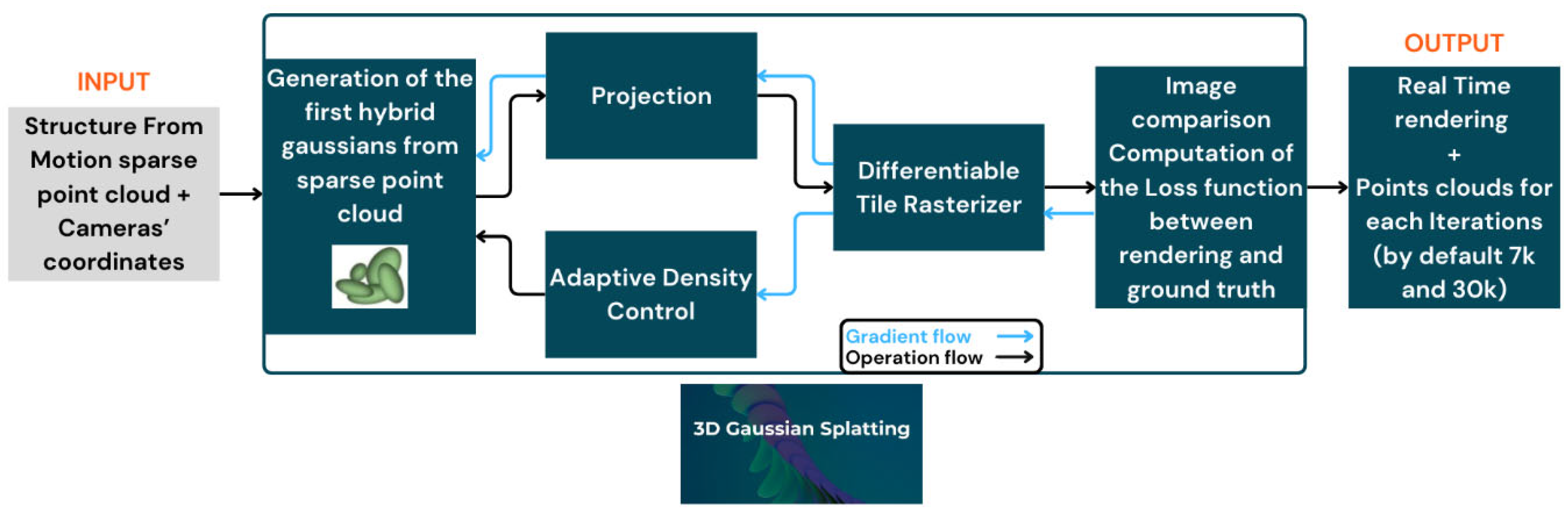
Figure 2.
Representative image pair: the left panel displays the original RAW capture, while the right panel demonstrates the result after AI masking.
Figure 2.
Representative image pair: the left panel displays the original RAW capture, while the right panel demonstrates the result after AI masking.
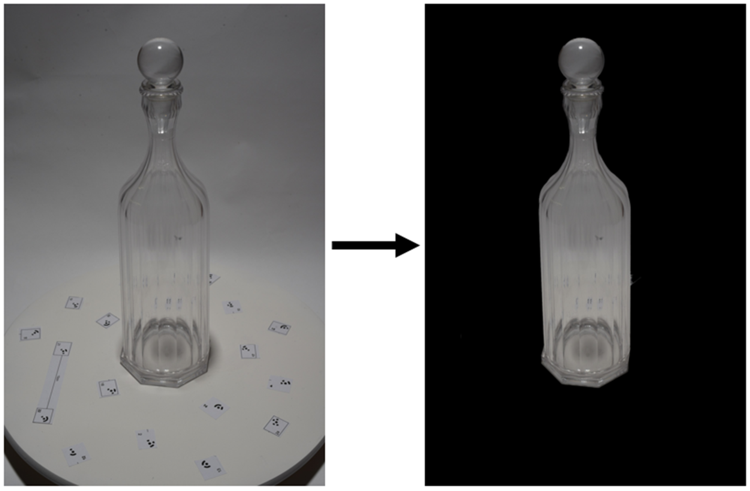
Figure 3.
Overview of the proposed methodology.
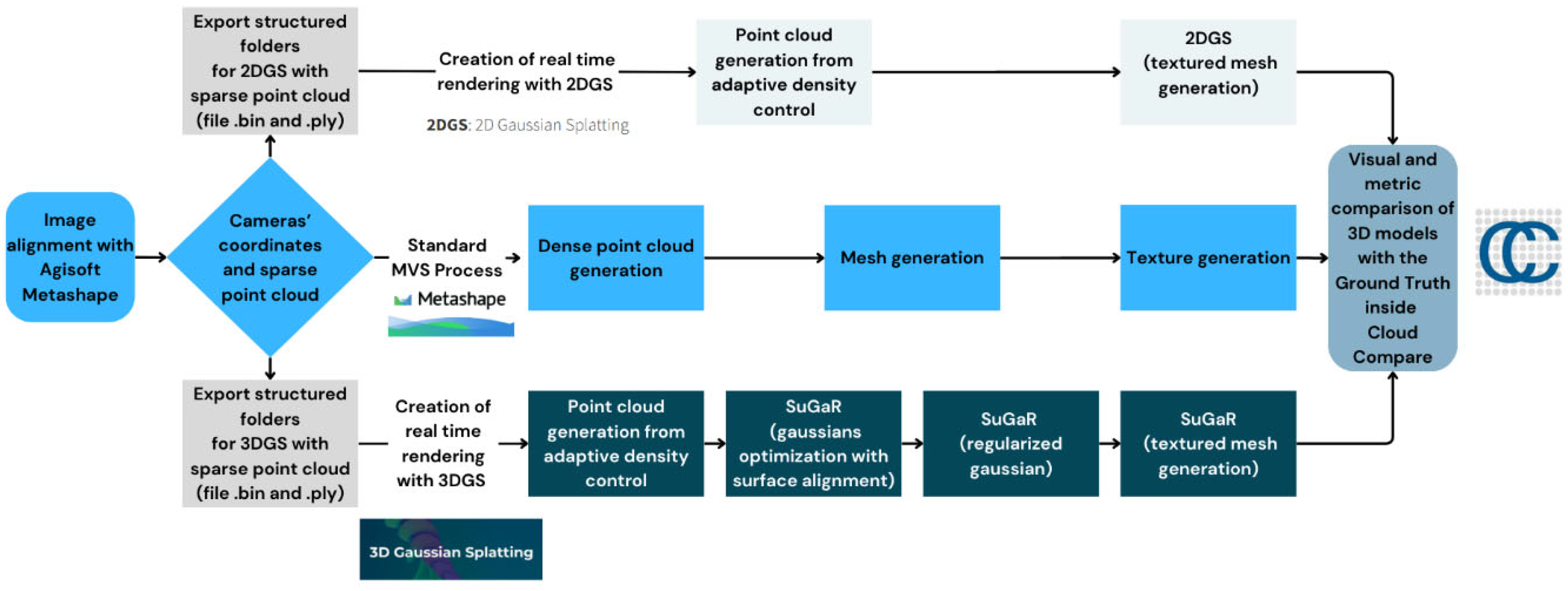
Figure 4.
Comparison of 3DGS and 2DGS. 3DGS utilizes different intersection planes P1 and P2 for value evaluation when viewing from different viewpoints, resulting in inconsistency. 2DGS provides multi-view consistent value evaluations.
Figure 4.
Comparison of 3DGS and 2DGS. 3DGS utilizes different intersection planes P1 and P2 for value evaluation when viewing from different viewpoints, resulting in inconsistency. 2DGS provides multi-view consistent value evaluations.
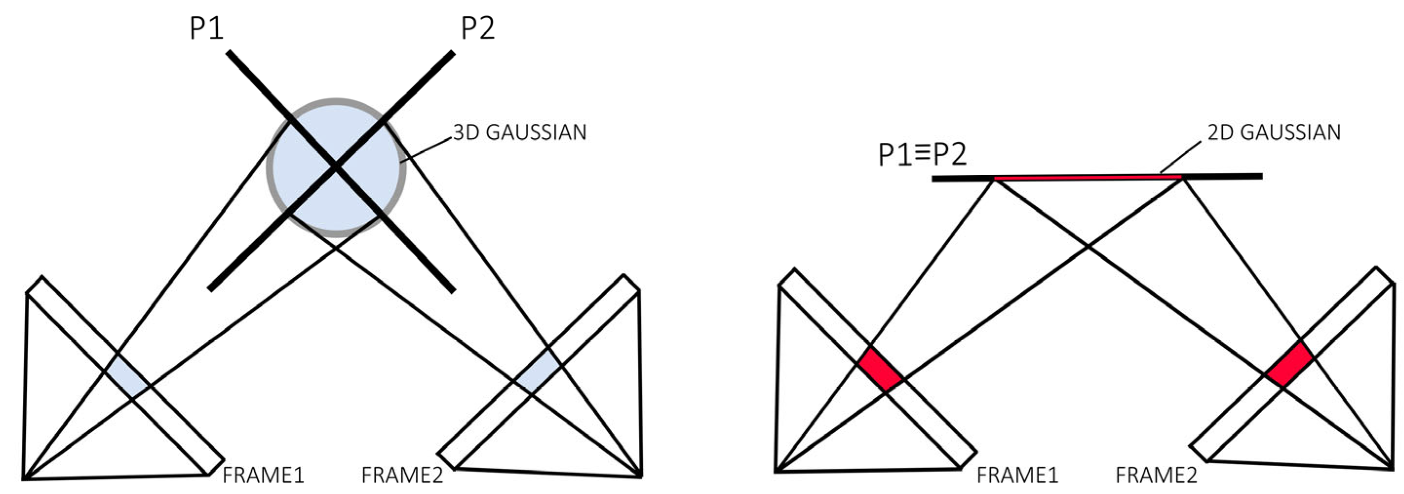
Figure 5.
Visual comparisons of the meshes reconstructed by the three different processes.
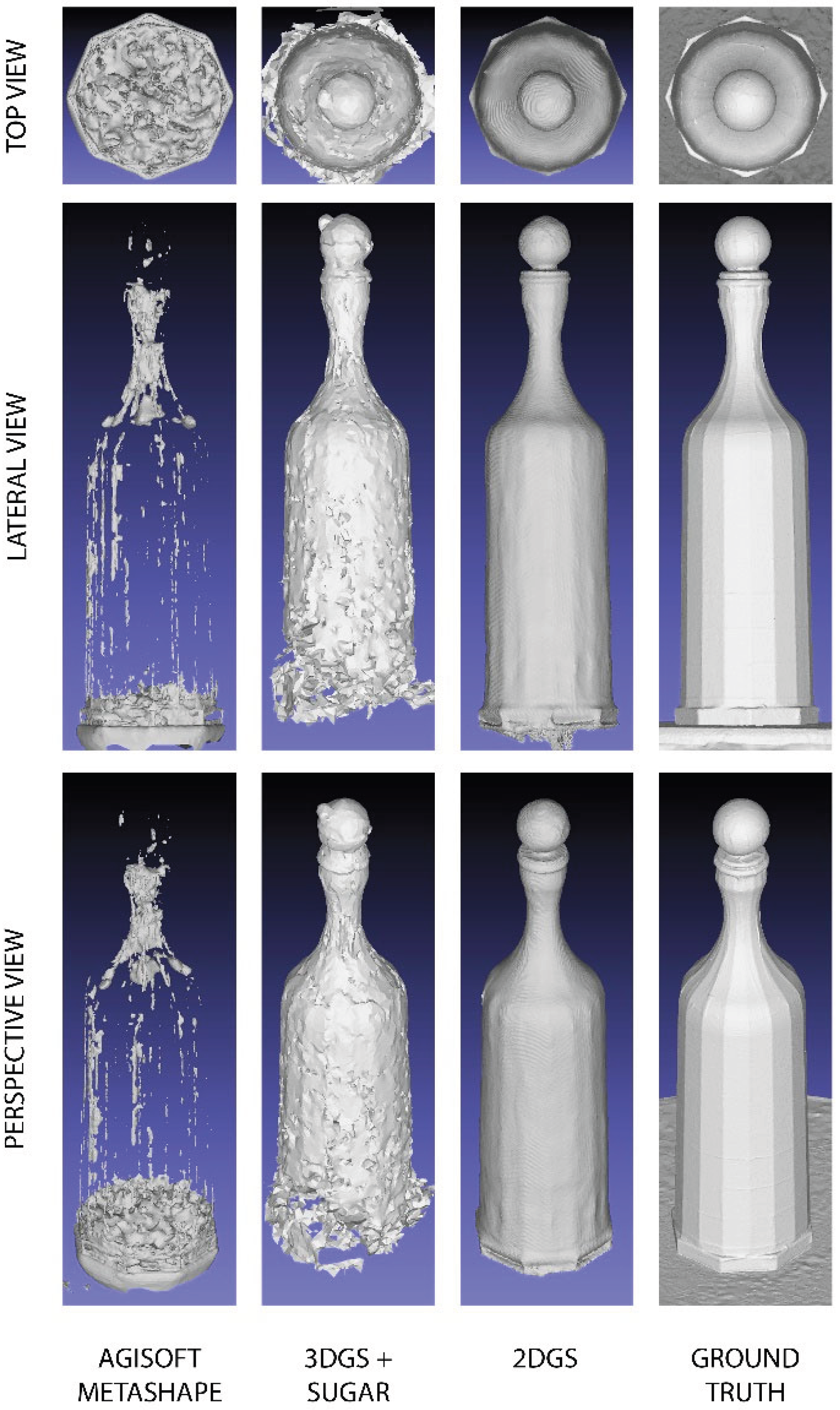
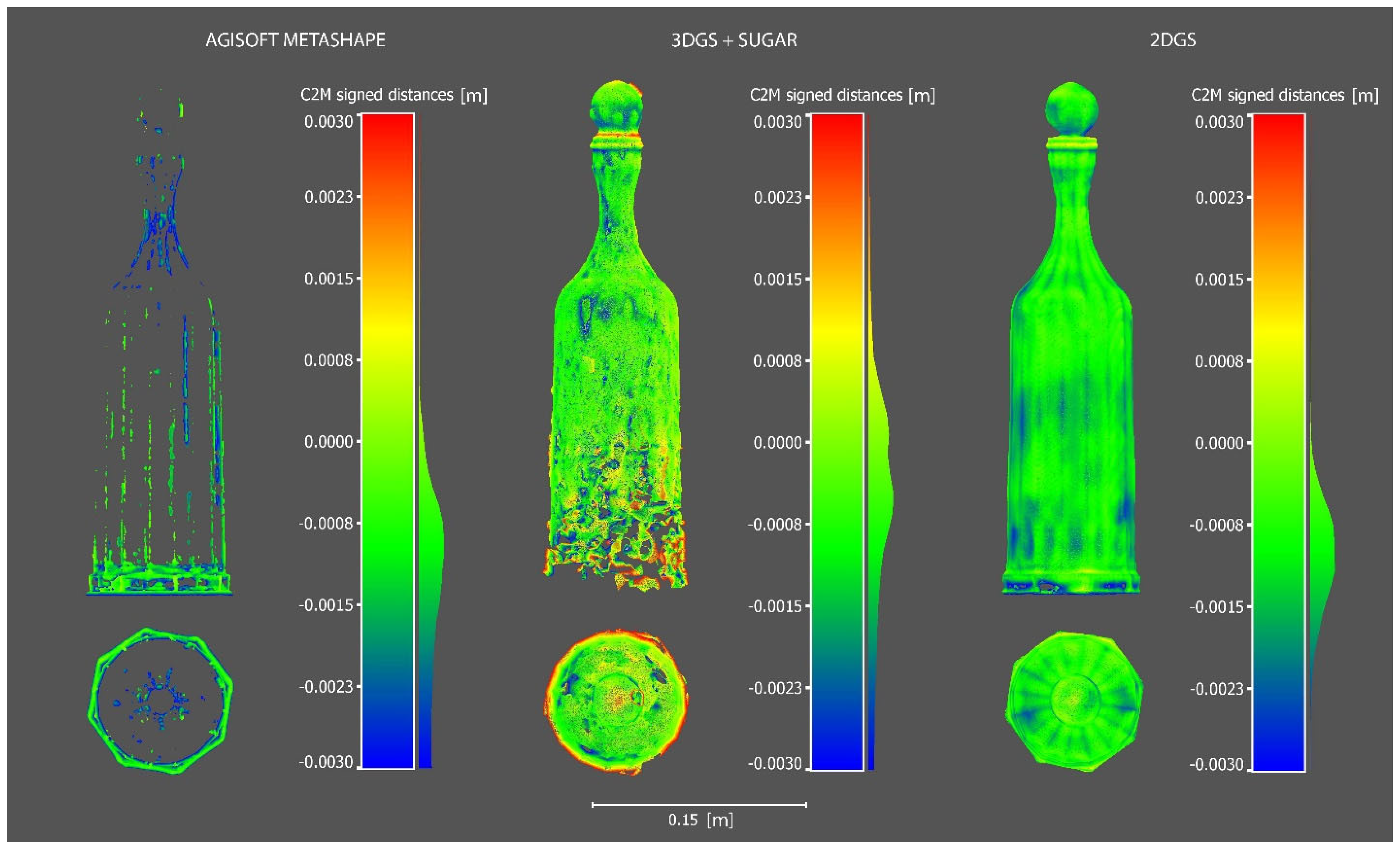
Figure 7.
Histogram of the C2M analysis of the 2DGS model considering outliers and in range points; a bimodal distribution curve is observed.
Figure 7.
Histogram of the C2M analysis of the 2DGS model considering outliers and in range points; a bimodal distribution curve is observed.

Figure 8.
Section of the 2DGS bottle model (bottom view).
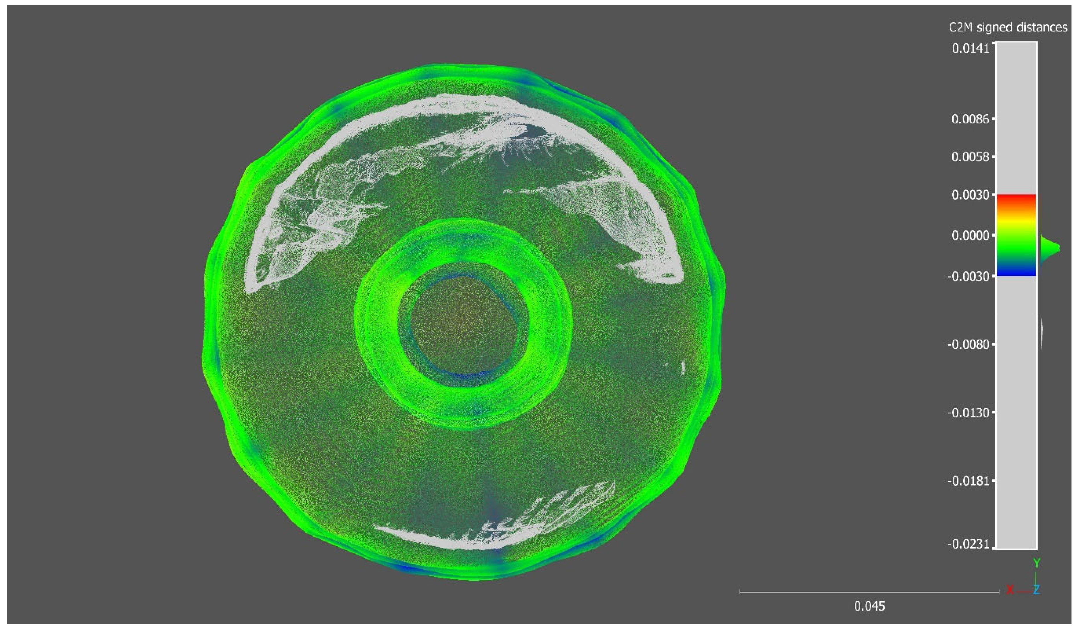
Figure 9.
Section of the 2DGS bottle model (axonometric view).
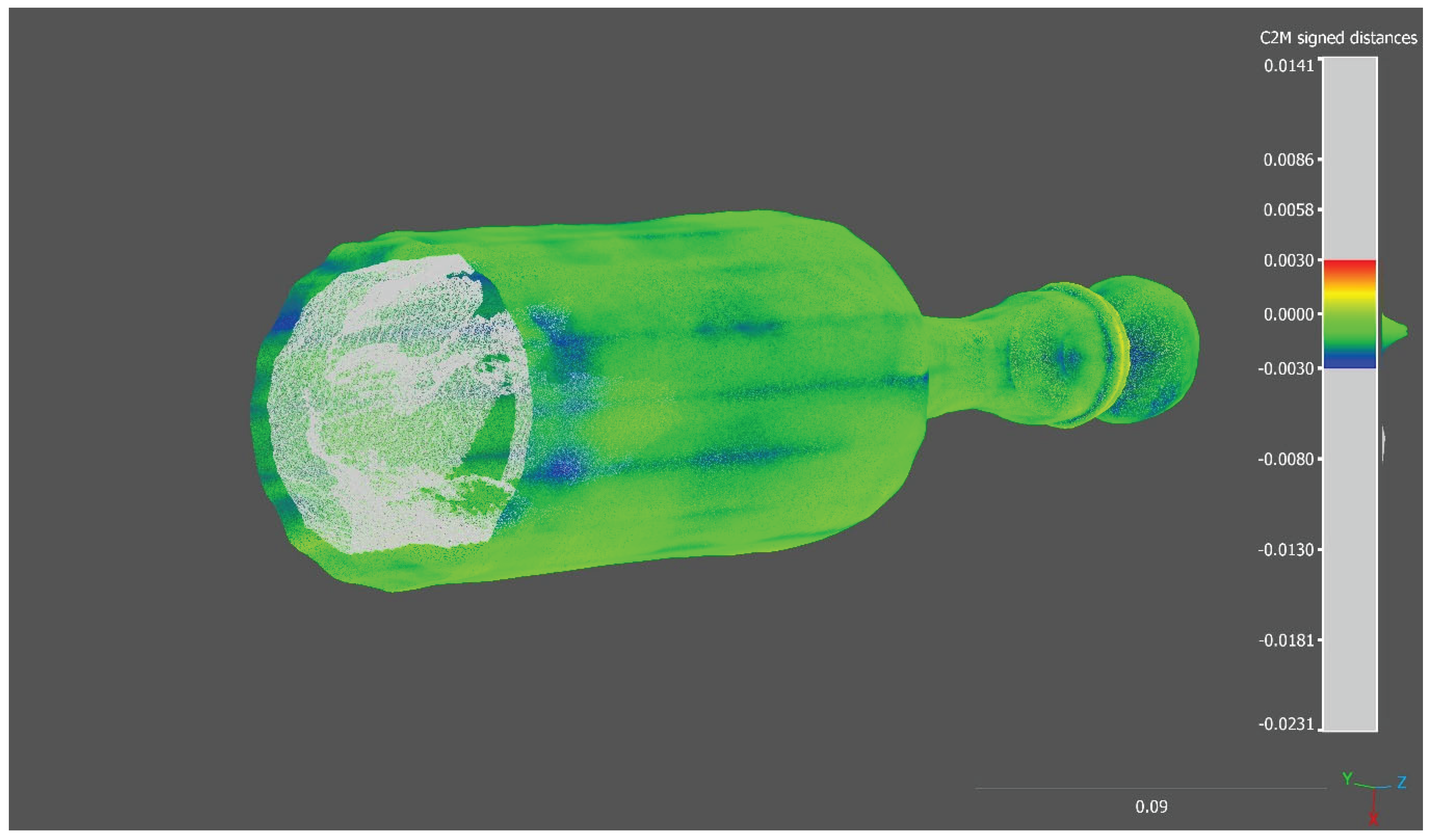
Figure 10.
Planimetric C2M slice section of the three generated models using as reference the ground truth (black profile).
Figure 10.
Planimetric C2M slice section of the three generated models using as reference the ground truth (black profile).
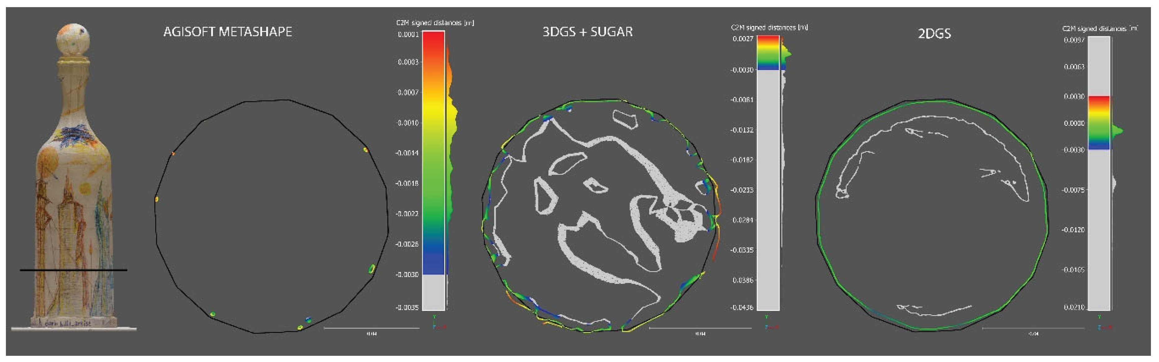
Figure 11.
Trasversal C2M slice section of the three generated models using as reference the ground truth (black profile).
Figure 11.
Trasversal C2M slice section of the three generated models using as reference the ground truth (black profile).
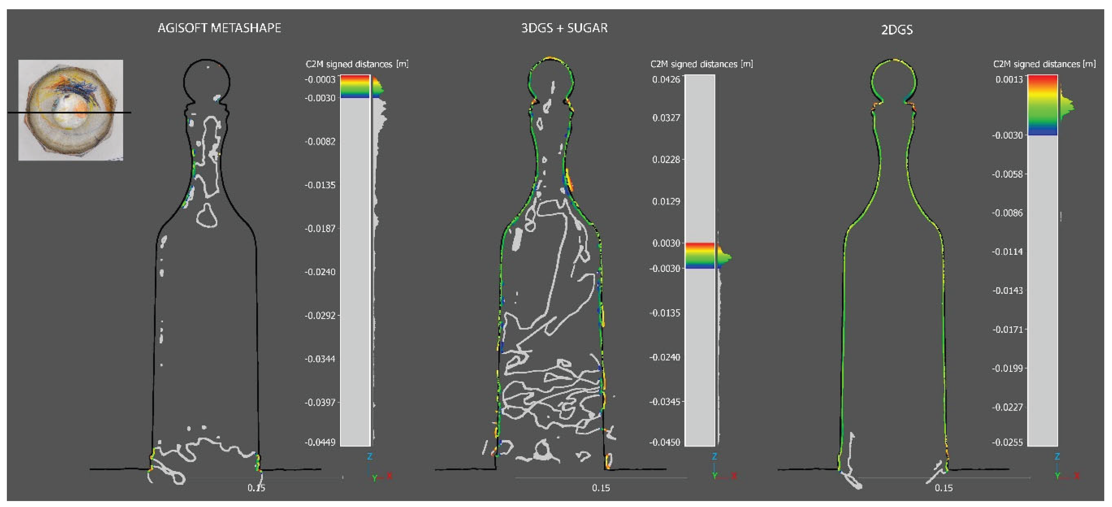
Figure 12.
Processing times for each parallel process.
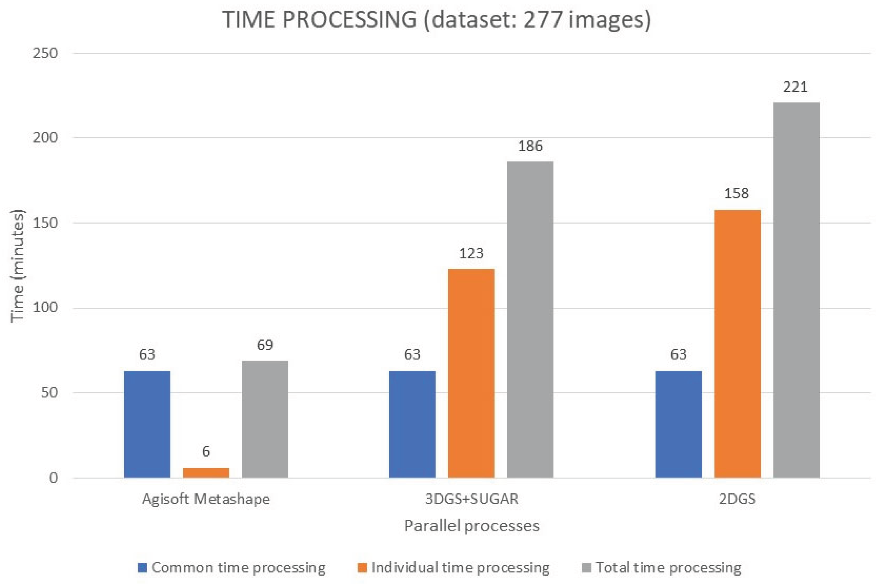
Table 1.
Metric quality thresholds.
| Metric | Range | Interpretation |
|---|---|---|
| SSIM | > 0.98 | Excellent structural similarity |
| 0.95 – 0.98 | High quality | |
| 0.90 – 0.95 | Good quality | |
| < 0.90 | Noticeable structural degradation | |
| PSNR | > 40 | Very high visual fidelity |
| 35 – 40 | High quality | |
| 30 – 35 | Medium / acceptable quality | |
| < 30 | Perceptible degradation | |
| LPIPS | < 0.05 | Excellent perceptual similarity |
| 0.05 – 0.10 | High perceptual quality | |
| 0.10 – 0.20 | Medium quality | |
| > 0.20 | Low perceptual fidelity / perceptible error |
Table 2.
Camera’s characteristics.
| Name | Image dimension | Focal lenght | Sensor dimensions |
|---|---|---|---|
| Nikon D750 | 6016x4016 pixels | 50 mm | W=36.0 mm H=23.9 mm |
Table 3.
Common settings of image acquisition.
| Aperture | Shutter speed range (Aperture priority mode) | ISO | Format |
|---|---|---|---|
| f/16 | 1/8 – 1/10 | 200 | RAW |
Table 4.
Common alignment parameters.
| Accuracy | Limit key points | Limit tie points | Generic preselection | Reference preselection | Adaptive camera model fitting | Exclude stationary tie points | Guided image matching |
|---|---|---|---|---|---|---|---|
| High | 0 | 0 | No | No | No | Yes | No |
Table 5.
Agisoft Metashape parametrs to generate mesh model.
| Source data | Surface type | Quality | Face count | Interpolation | Depth filtering |
|---|---|---|---|---|---|
| Depth Maps | Arbitrary | High | High | Enabled | Mild |
Table 8.
Rendering metrics PSNR LLPIS and SSIM (visual fidelity), for 3DGS and 2DGS compared with the mesh accuracy.
Table 8.
Rendering metrics PSNR LLPIS and SSIM (visual fidelity), for 3DGS and 2DGS compared with the mesh accuracy.
| Method | SSIM | PSNR | LPIPS | Visual Fidelity | Mesh Accuracy |
|---|---|---|---|---|---|
| 3DGS | 0.9768 | 36.06 | 0.0629 | ☑ Higher (more realistic) | ✖ Low degree of conformity |
| 2DGS | 0.9734 | 34.91 | 0.0696 | ☑ Good, slightly worse | ☑ High degree of conformity |
Table 9.
Overview of the different computational resources utilized by 2DGS, 3DGS, and Agisoft Metashape.
Table 9.
Overview of the different computational resources utilized by 2DGS, 3DGS, and Agisoft Metashape.
| Software/Process | CPU Usage | GPU Usage | Notes |
|---|---|---|---|
|
Agisoft Metashape |
☑ Important |
☑ Important |
- CPU used for feature matching, mesh generation, and texturing. - GPU accelerates depth maps, point cloud, and rendering. |
|
3DGS + SUGAR |
✖ Minimal |
☑ Primary |
- Intensive GPU computation for 3D Gaussian management. - CPU marginally used for coordination. |
|
2DGS |
✖ Minimal |
☑ Primary |
- Uses GPU for rasterization and Gaussian optimization. - CPU involved only in data management. |
Disclaimer/Publisher’s Note: The statements, opinions and data contained in all publications are solely those of the individual author(s) and contributor(s) and not of MDPI and/or the editor(s). MDPI and/or the editor(s) disclaim responsibility for any injury to people or property resulting from any ideas, methods, instructions or products referred to in the content. |
© 2025 by the authors. Licensee MDPI, Basel, Switzerland. This article is an open access article distributed under the terms and conditions of the Creative Commons Attribution (CC BY) license (http://creativecommons.org/licenses/by/4.0/).
Copyright: This open access article is published under a Creative Commons CC BY 4.0 license, which permit the free download, distribution, and reuse, provided that the author and preprint are cited in any reuse.


