
Submitted:
07 August 2024
Posted:
08 August 2024
You are already at the latest version
Abstract
This study analyzes future hydrological droughts in LCKW using the SWAT model and data from 2010-2021, evaluating the Streamflow Drought Index (SDI) for 5, 10, 25, and 50-year return periods (RP) for 2029 and 2039 under RCP4.5 and RCP8.5 scenarios. The model shows high accuracy (R² = 0.82, NSE = 0.78). Under RCP4.5, streamflow may increase by 34.74% and 18.74%, while RCP8.5 predicts significant decreases of 37.06% and 55.84%. Historical data reveal frequent short-term droughts during SDI-3, notably in 2014–2016 and 2020–2021, with SDI-6 indicating less frequent but severe droughts, especially in 2015 and 2020. Future projections under RCP8.5 suggest wors-ening drought conditions in 2029 and 2039, with critical drought periods from January to April and November. Wavelet analysis indicates a high risk of severe hydrological drought in LCKW due to low annual recurrence rates, with the highest drought severity over a 50-year RP. The study high-lights an increasing likelihood of frequent and severe droughts, particularly under high emission scenarios such as RCP8.5, which could result in significant water shortages and ecosystem disrup-tions. It emphasizes the significance of adaptive water resource management strategies in mitigating negative impacts on water security and ecosystem health.
Keywords:
climate change
; CMIP5
; Hydrological Drought Characteristics
; Streamflow Drought Index (SDI)
1. Introduction
Climate change significantly impacts extreme events [1], particularly droughts [2], which have long-lasting impacts on human life, the environment, industry, and the economy [3]. Hydrological droughts, characterized by below-average streamflow, are crucial for water resource planning and management due to increasing demand and population growth [4]. Predicting future droughts is essential due to climate change’s nonstationary nature, which affects efficient water resource management, irrigation system operation, agricultural production, and national economic stability [5].
Northeastern Thailand has been significantly impacted by climate change, resulting in decreased rainfall and streamflow, with studies projecting a 13–19% decrease in annual streamflow and shifts in seasonal flow patterns [6]. This has severely affected the agricultural sector, particularly rice farming, with projections indicating a decline in rainfed rice yields due to higher temperatures and altered rainfall patterns [7]. Climate change is increasing drought severity, emphasizing the need to consider different climate change scenarios when assessing hydrological droughts [8]. The Intergovernmental Panel on Climate Change (IPCC) and the Coupled Model Intercomparison Project (CMIP) are developing models to predict future climate change, with the CMIP5 dataset showing improved performance in simulating global precipitation trends. [9].
Climate change is significantly impacting the Lam Chiang Kri watershed (LCKW) in Thailand [10], with geographical limitations such as a plateau alternating with geographical limitations [11]. Additionally, the predominantly sandy soil in the region does not retain water well [12]. These factors lead to severe agricultural impacts, as crops primarily depend on rainfall. For instance, rice production in 2015 saw a 24.52% decrease due to the strong El Niño [13]. Historical and contemporary studies highlight the region’s climatic variability, frequent droughts, and issues like soil erosion and salinity, all of which impact agricultural productivity. The transition from highly productive environments to arid conditions emphasizes the need for sustainable water resource development and improved agricultural practices. Efforts must focus on mitigating the adverse effects of climatic changes and human activities to ensure the region’s long-term viability and productivity [14,15,16,17]. There is a gap in the literature regarding hydrological drought characterization across different return periods combined with climate change scenarios. Incorporating return periods and climate change scenarios for future hydrological drought prediction is crucial for holistic planning and effective water management. Water managers and organizations are encouraged to use available tools and scientific understanding to develop new strategies for water resource conservation.
This study aims to evaluate the impact of climate change on streamflow, assess the hydrological drought index, and characterize hydrological drought across different return periods in the semi-arid climate of northeastern Thailand. The methodology involves using the SWAT model, a widely used hydrological model for simulating streamflow, driven by downscaled climate projections from appropriate GCMs under RCPs for two emission scenarios: RCP4.5 and RCP8.5. The downscaled results for years 2029 and 2039 will be analyzed. The study includes observational streamflow data for the reference period, uses SWAT models to estimate future streamflow, and calculates hydrological drought. The research background, purpose, methodology, results, and discussions are presented in subsequent sections.
2. Materials and Methods
2.1. Study Area
The Lam Chiang Kri Watershed (LCKW) is in northeastern Thailand, within the Isan Plateau, and serves as the upper branch watershed of the Mun Watershed. It covers 2,959.59 square kilometers and has an elevation range of 145 meters to 593 meters above sea level (Figure 1) [18]. The elevation ranges from 145 meters to 593 meters above sea level, with terrain sloping from west to east. The soil is predominantly laterite, a type of sandy loam with poor water-retention capabilities. Hydrographs in this region display sharp rising limbs, high peaks, and steep recess limbs, indicating that rainfall quickly runs off rather than soaking into the ground, leading to rapid changes in streamflow levels [19].
An analysis of land use data from the Land Development Department (LDD) of Thailand shows that about 88.89% of the LCKW comprises agricultural areas, but only 22.09% of them are equipped for irrigation. There is a high drought risk area of 1,338.34 square kilometers (45.89% of the total area), a moderate drought risk area of 866.84 square kilometers (29.72% of the total area), and a low drought risk area of 711.45 square kilometers (24.39% of the total area). This data underscores the area’s vulnerability to drought, which severely impacts local agriculture and water resources.
The LCKW, situated in the semi-arid climate of northeastern Thailand [15,20], experiences lower rainfall and higher temperatures compared to other parts of the country. According to data from the Thai Meteorological Department (TMD), the average annual rainfall is 947.66 mm, and the average annual temperature is 33 °C. The LCKW experiences distinct wet and dry seasons influenced by monsoons [21]. The Southwest monsoon brings warm, moist air from the Indian Ocean, causing heavy rainfall during the rainy season from mid-May to mid-October. The northeast monsoon causes the dry season from mid-October to mid-February. The transitional period between monsoons is from mid-February to mid-May. According to data from the Royal Irrigation Department of Thailand (RID), the average annual streamflow in the LCKW is approximately 2,661.51 m³/s, with 91.78% occurring during the rainy season and the remainder during the dry season.
2.2. Methodology
This study utilized daily rainfall data from five gauges of the TMD, covering the years 1992–2022. Additionally, daily streamflow data from the gauge at M188 station for the period 2010–2021 was provided by RID. The locations of the gauges are illustrated in Figure 1, and a schematic diagram of the overall framework is shown in Figure 2. Historical and future periods were defined to assess the impact of climate change on hydrological droughts. Observed rainfall and streamflow data were used for the calibration and validation of the Soil and Water Assessment Tool (SWAT) model, as well as for calculating the baseline (2010-2021) hydrological drought index. After bias correction, the ability of the Regional Climate Models (RCMs) to generate streamflow during the baseline (2010-2021) was evaluated. The output from all selected RCMs was analyzed, with particular emphasis on the drought index results obtained from the best-performing RCM. Details regarding the SWAT modeling, RCM, and hydrological drought index calculations are provided in the following sections.
2.2.1. Regional Climate Model (RCM)
According to the American Meteorological Society (AMS), a regional climate model (RCM) is a numerical climate prediction model driven by specified lateral and ocean conditions from a general circulation model (GCM) or an observation-based dataset (reanalysis). It simulates atmospheric and land surface processes while accounting for high-resolution topographical data, land-sea contrasts, surface characteristics, and other components of the Earth system.
RCMs were developed to address the limitations of GCMs, which provide global estimates at a coarse spatial resolution of 100–300 km [22], and to enable studies of regional phenomena with finer spatial resolutions [23], currently ranging from approximately 50 km to 12 km [24]. Driven by lateral boundary conditions and reanalysis data, RCMs can account for local scale forcings, and processes influenced by complex topography, coastlines, inland bodies of water, and land cover distribution. With improved spatial resolution, RCMs provide more accurate climate information than GCMs and are widely used to study regional climate variability, climate extremes, and the impacts of climate change. The number of RCMs available from laboratories worldwide is continuously increasing. [25].
In this study, we analyzed precipitation data from CMIP5 models under the Representative Concentration Pathway (RCP) 4.5 scenario, where radiative forcing stabilizes at 4.5 W/m² corresponding to 650 ppm CO2-equivalent [26]. This scenario is considered a projection of moderate climate impact. Conversely, RCP 8.5 is regarded as a high-emission scenario, where radiative forcing stabilizes at 8.5 W/m² corresponding to 950 ppm CO2-equivalent [27,28,29]. The data was used to project future precipitation patterns. Global Circulation Models (GCMs), which are among the most reliable tools for climate prediction and simulation, were utilized for this purpose [30].
For our analysis, we selected three models: EC-Earth3, HadGEM2, and MPI-ESM-MR. We divided the climate data into two distinct periods for analysis: the 5th year (2029) and the 15th year (2039). Additionally, we compared the rainfall predictions from these GCMs with actual recorded rainfall data from 2004-2022 to evaluate the models’ accuracy in predicting future climatic conditions.
1) Taylor diagram
The Taylor diagram is a valuable tool in environmental sciences, particularly for visualizing the performance of models predicting variables like precipitation. It combines three key metrics: correlation coefficient (r), root mean square error (RMSE), and standard deviation (SD), into a single graphical representation. This allows for a quick comparison of how well different models capture the correlation, variability, and overall accuracy of the observed data. However, the Taylor diagram can be limited in its ability to represent certain types of errors [31].
To address these limitations, researchers have proposed extensions to the Taylor diagram. These extensions may incorporate additional metrics, such as bias, to provide a more comprehensive picture of model performance. In this study, we plan to utilize the Taylor diagram to compare the performance of the three chosen RCMs in simulating future precipitation patterns. By analyzing the location of each model’s point on the diagram, we can gain insights into how well each model replicates the observed rainfall variability, correlation with the observations, and overall agreement in terms of standard deviation [32].
2.2.2. SWAT Model
1) Model Description
The SWAT model, developed by the USDA, is a process-based, semi-distributed, and continuous-in-time watershed hydrological model [33] that is crucial for watershed simulation, especially in the context of climate change. It analyzes soil profiles and water routing within watersheds, calculates interflow using a linear function [34], and integrates GIS with DEM and raster functions for enhanced accuracy [35]. The model incorporates various datasets, including terrain, land use, soil, and meteorological data. Multi-temporal observed streamflow data is necessary for calibration and validation.
In this study, the SWAT model was used to delineate the watershed, divide it into sub-watersheds, and create hydrologic response units (HRUs) based on land use, soil type, and slope data. Thailand’s Land Development Department classified land use into twelve main types, and the soil map identified forty-four soil types in the study area. The slope classifications include flat (0–2%), sloping (2–5%), hilly (5–15%), steep (15–35%), and very steep (>35%).
A water balance equation was the basis for the SWAT model. represented as follows Equation (1):
where and (mm) are the initial and final soil water on a given day, , , and (mm) are the rainfall, runoff, ET, water seepage to the upper soil layer, and return flow on that day, respectively.
The SWAT model used the Soil Conservation Service Curve Number (SCS-CN) approach to compute surface runoff in the study area. The SCS-CN equation is shown by Equation (2), as follows:
where is daily surface runoff (mm); is daily rainfall depth (mm); is the initial abstraction (mm); and is the retention parameter (mm). The retention parameter
S is not fixed and can be affected by factors such as slope, soil, and land use management. Mathematically, the retention parameter can be represented as Equation (3), as follows:
where is the retention parameter (mm), and is the curve number. The curve number ranges from 0 to 100, with 100 indicating no potential retention and 0 reflecting infinite potential retention [36].
2) Model Setup
The SWAT model calibration and validation process requires careful consideration of observation streamflow data from the M188 station. The data is divided into 80% for calibration and 20% for validation, with periods selected from 2010 to 2021. The simulation runs for 12 years, starting from January 1, 2010, to December 31, 2021. Nine sub-watersheds were created in the study area, with a threshold of 10% for land use, 10% for soil, and 10% for slope, resulting in 108 Hydrologic Response Units.
3) Model Evaluation
The study used SWAT-CUP software with the Sequential Uncertainty Fitting (SUFI) algorithm to calibrate a model [37], which can handle a large number of parameters and combine sensitive analysis and improvement [35].
The model’s performance was compared using three statistical performance indices: Nash and Sutcliffe Efficiency (NSE) following equation (4) [38], the coefficient of determination (R²) following equation (5) [39], percent bias (PBIAS) following equation (6) [40], and Kling–Gupta Efficiency (KGE) following equation (7) [41], to evaluate its daily stream-flow performance during calibration and validation phases.
and represent observed and simulated values, respectively. The NSE value of the model should be more than 0.50, while the R² should be at least 0.7. PBIAS should not exceed 25 percent to be acceptable. KGE can be categorized as good (KGE ≥ 0.75), intermediate (0.75 > KGE ≥ 0.5), poor (0.5 > KGE > 0), and very poor (KGE ≤ 0).
2.2.3. Hydrological Drought Index and Hydrological Drought Characteristics
The Streamflow Drought Index (SDI) is a tool used to assess the severity of hydrological droughts. Positive SDI values indicate wetter conditions, while negative values indicate hydrological drought. The SDI is used to identify and assess drought events across various time frames, including dry and wet seasons. It is calculated using monthly streamflow data, enabling effective management of drought and water resource scarcity over different time scales. The choice of time scale depends on the specific aspect of the drought being examined. Shorter periods (3 months) are ideal for tracking agricultural droughts and their impact on crops, while longer periods (6 months) provide insight into hydrological droughts affecting surface and groundwater resources. Analyzing both time scales offers a more comprehensive understanding of drought conditions [42]. These choices can be further refined based on the climate and water resource focus of the study area, as outlined in Equation 8:
Where represents the cumulative streamflow volume for period n and quarter and q while and are the mean and the standard deviation of cumulative streamflow volumes of the reference period, respectively. The classification of hydrological drought based on the SDI (Table 1) offers a detailed understanding of drought characteristics.
The Theory of Runs (ToR) is a statistical method used to analyze drought characteristics [44], including drought event (DE), drought duration (DD), drought severity (DS), and drought intensity (DI) (Figure 3). DE is identified when the SDI value falls below a critical threshold. DD represents the duration of drought in months with negative SDI values, while DS is the sum of the absolute values of the SDI during a DE. DI can be defined as the absolute lowest value of the index (DI1) or the ratio of DS to DD in a DE (DI2).
2.2.4. Scenarios analysis in Different Return Periods
The CumFreq software (https://www.waterlog.info/cumfreq.htm; accessed on January 28, 2024) was used to determine the most suitable distribution for a drought characterization time series across different return periods (5, 10, 25, and 50 years) and two time scales (3 and 6 months). This cumulative frequency analysis tool uses multiple probability distribution functions to recommend the most appropriate type based on the input data [46]. The absolute values of the SDI were input into CumFreq, and various statistical distributions were obtained. Wavelet analysis was used to assess SDI values at different time scales over various return periods. A geostatistical approach was employed to interpolate streamflow and SDI values into contour maps, ensuring accurate variogram models are essential for interpreting natural phenomena [47]. The relationship between streamflow and absolute SDI was also analyzed using Surfer 21.1.158 software, which is used to create three-dimensional diagrams with contour lines based on the Kriging interpolation method. [48].
3. Results
The investigation of critical hydrological droughts in the Lam Chiang Kri Watershed (LCKW) under CMIP5 climate change scenarios is divided into three key areas: calibration and validation of the SWAT model, identification of historical drought characteristics, and assessment of climate change impacts on hydrological drought. These areas are detailed as follows:
3.1. Calibration and Validation of the SWAT Model
The SWAT model simulation from 2010 to 2021, supported by data from a hydrological station within the Lam Chiang Kri Watershed, effectively analyzed the watershed’s hydrological responses to varying meteorological conditions. Calibration and validation using the SUFI-2 algorithm within SWAT-CUP ensured the accuracy of streamflow patterns, significantly enhancing the reliability of the results. Sensitivity analysis identified five critical parameters—CN2, ESCO, SOL_AWC, GW_DELAY, and SLSUBBSN—highlighting their significant influence on streamflow simulation (Table 2). These findings provide a robust foundation for future water resource management and drought mitigation strategies in LCKW.
The calibration and validation phases of the SWAT model development depend on accurate observed streamflow data. For this study, data from station M188, covering the period from 2010 to 2021, was utilized. Figure 4 shows that the calibrated SWAT model at station M188 closely matched the observed data patterns.
For statistical evaluation, R², NSE, PBIAS, and KGE values were used. Throughout the calibration and validation periods, the streamflow stations exhibited R² and NSE values above 0.75, indicating good to very good performance. PBIAS values were maintained below 25%, aligning with the preferred threshold. KGE values were classified in the intermediate category, as detailed in Table 3.
3.2. Identification of Historical Drought Characteristics
The historical drought characteristics in LCKW were calculated using the SDI, focusing on 3-month (SDI-3) and 6-month (SDI-6) accumulation periods. The SDI-3 indicates frequent, short-term drought events occurring almost annually, with significant droughts around 2014–2016 and 2020–2021, and the SDI-6 indicates less frequent but more severe and prolonged droughts, particularly noticeable in 2015 and 2020. (Figure 5).
The analysis indicates an average of 2.67 drought events per year, with a maximum duration of 3 months and a peak severity of -31.97. The SDI-6 period reveals less frequent yet more severe and prolonged droughts, notably in 2015 and 2020, with an average of 1.25 drought events per year, a maximum duration of 6 months, and a peak severity of -43.04. Both indices underscore the persistent and recurrent nature of drought conditions, highlighting the necessity for effective water resource management strategies to mitigate both short-term and medium-term drought risks. The maximum intensity for SDI-3 was -2.44 (DI1) and -1.35 (DI2), whereas for SDI-6, it was -2.74 (DI1) and -1.69 (DI2). (Table 4)
The results indicate the persistent and recurrent nature of drought conditions in the LCKW region. Short-term (3-month) periods tend to have more frequent but less severe droughts, while longer-term (6-month) periods show fewer but more severe and prolonged droughts, notably in the years 2015 and 2020.
3.3. Assessment of Climate Change Impacts on Hydrological Drought
The assessment of climate change impacts on hydrological droughts using the projected rainfall model from CMIP5 under two scenarios, RCP4.5 and RCP8.5, is explained as follows:
3.3.1. Selecting the Fittest GCM
To estimate the effects of climate change on rainfall during the simulation and reference periods (1992-2005), this study utilized three CMIP5 GCMs: EC-Earth3, HadGEM2, and MPI-ESM-MR, under the RCP4.5 and RCP8.5 scenarios. The Taylor diagram was employed to assess the fit of these models. Among them, the EC-Earth3 model (red dot) demonstrated the highest correlation with observed data, with a correlation coefficient of 0.65, a standard deviation (SD) of 1.98, and a root mean square error (RMSE) of 3.41, making it the most accurate model. The HadGEM2 model (blue dot) also showed a strong correlation but had a higher RMSE. The MPI-ESM-MR model (green dot) exhibited moderate correlation and RMSE values. (Figure 6).
3.3.2. Future Rainfall
The future rainfall analysis compared monthly averages from observed periods with projections under the RCP4.5 and RCP8.5 scenarios. Figure 7 presents the EC-Earth3 model’s average monthly rainfall predictions for 2029 and 2039, alongside the baseline data from 2004–2022 (Table 5), to evaluate changes under both climate scenarios.
In 2029 (the 5th year) under the RCP4.5 scenario, the projected annual rainfall totals 1,311.94 mm, with the highest monthly rainfall occurring in August (383.03 mm) and the lowest in January (11.46 mm). This represents a predicted increase of 38.44% in future rainfall compared to the baseline. Under the RCP8.5 scenario, the projected annual rainfall is 892.97 mm, with the highest in August (215.53 mm) and the lowest in February (11.90 mm), indicating a decrease of 5.77% from the baseline (2004–2022).
In 2039 (the 15th year) under the RCP4.5 scenario, the projected annual rainfall is 1,101.06 mm, with the highest monthly rainfall in July (248.36 mm) and the lowest in January (14.80 mm), marking a 16.19% increase from the baseline. Under the RCP8.5 scenario, the projected annual rainfall totals 805.46 mm, with the highest in October (218.96 mm) and the lowest in January (1.33 mm), reflecting a 15.00% decrease from the baseline (2004–2022).(Table 5)
The results highlight significant disparities in the variability of monthly rainfall between the two future time frames, with more pronounced changes observed in 2039, especially under the RCP8.5 scenario, where the steepest declines in rainfall are projected. This research emphasizes the distinct variations in annual and seasonal rainfall patterns produced by different climate change scenarios.
3.3.3. Future Streamflow
This study analyzed variations in streamflow by comparing historical data with model simulations, focusing on mean annual streamflow under the RCP4.5 and RCP8.5 climate scenarios. Figure 8 presents the predicted average monthly streamflow for 2029 and 2039, compared to the baseline period of 2010-2021 (Table 6), to evaluate potential changes under each scenario.
In 2029 (the 5th year) under the RCP4.5 scenario, the annual streamflow is projected to be 3,623.09 m³/s, with the highest flow occurring in October (1,495.52 m³/s) and the lowest in February and March (0.13 m³/s). The monsoon season contributes 86.97% (3,150.93 m³/s) of the total, while the dry season contributes 13.03% (472.17 m³/s), indicating a 34.74% increase from the baseline (2010-2021). Under the RCP8.5 scenario, the streamflow is projected to drop to 1,692.38 m³/s, with the highest flow in October (708.20 m³/s) and no flow in February and March. The monsoon season contributes 85.10% (1,440.29 m³/s) of the total, and the dry season contributes 14.90% (252.09 m³/s), representing a 37.06% decrease from the baseline (2010-2021). (Table 6)
In 2039 (the 15th year), under the RCP4.5 scenario, the projected streamflow is 3,192.18 m³/s, with October again having the highest flow (1,495.52 m³/s) and March and April the lowest (9.66 m³/s). The monsoon season contributes 86.54% (2,762.47 m³/s) and the dry season 13.46% (429.71 m³/s), an 18.71% increase from the baseline. Under the RCP8.5 scenario, streamflow is projected to further decrease to 1,187.54 m³/s, with peak flow in August (378.82 m³/s) and the lowest in April (0.19 m³/s). The monsoon season contributes 95.93% (1,139 m³/s) and the dry season 4.06% (48.33 m³/s), indicating a 55.84% decrease from the baseline (2010-2021).
The results highlight significant disparities in the variability of monthly rainfall between the two future time frames, with more pronounced changes observed in 2039, especially under the RCP8.5 scenario, where the steepest declines in rainfall are projected. This research emphasizes the distinct variations in annual and seasonal rainfall patterns produced by different climate change scenarios.
3.3.4. Future Hydrological Drought Characteristics
The future hydrological drought characteristics, as projected by the SDI for the years 2029 and 2039, are analyzed under two climate scenarios: RCP4.5 and RCP8.5. These projections are based on 3-month (SDI-3) and 6-month (SDI-6) accumulation periods (Figure 9), and are detailed as follows:
The analysis shows that in 2029, the SDI-3 under RCP4.5 indicates drier conditions from January to April, with improvements from May to September, and a decline towards the year’s end. The RCP8.5 scenario follows a similar pattern but with more severe droughts. For SDI-6, both scenarios exhibit dry conditions early in the year, some recovery mid-year, and a decline towards year-end, with RCP8.5 showing more intense droughts. By 2039, both SDI-3 and SDI-6 projections under RCP4.5 and RCP8.5 suggest worsening droughts, particularly under RCP8.5, with severe droughts expected from January to April and in November. The projections highlight an increasing trend of drought in-severity and frequency, especially under the higher emission scenario (RCP8.5), emphasizing the urgent need for effective water management and climate adaptation measures to mitigate the adverse impacts of these projected changes.
3.3.5. Analysis of SDI in Different Return Periods
The results analyze the relationship between streamflow and the absolute SDI across different return periods and time scales using wavelet analysis. The diagrams display return periods on the horizontal axis and average streamflow on the vertical axis, with iso-lines representing various levels of drought severity (Figure 10). Bold blue lines indicate low drought severity, while bold red lines signify high severity.
For SDI-3, return periods of 2–10 years exhibit higher drought severity, with SDI values ranging from 2.08 to 2.86, indicating more severe droughts over shorter periods. In contrast, longer return periods (over 10 years) experience smaller, shorter droughts. Under the RCP4.5 scenario, the most severe droughts are observed in return periods of 10–15 years, with an absolute SDI value of 2.56 for the 50-year return period. Conversely, the RCP8.5 scenario shows more severe and widespread droughts, particularly in return periods of 25–50 years, with absolute SDI values ranging from 2.26 to 4.34. Return periods of 1–25 years under RCP8.5 also show moderate drought severity across most of the watershed area.
For SDI-6, the study found that return periods of 10–50 years exhibit the greatest drought severity, with absolute SDI values ranging from 2.24 to 2.74. These severe droughts cover longer periods and have a relatively long duration. In shorter return periods of 1–10 years, fewer droughts are observed. Under the RCP4.5 scenario, severe droughts are primarily seen in the 25–50 year return period, with absolute SDI values ranging from 2.31 to 3.76, indicating continuous drought severity over a long period. For return periods of 0–10 years, no droughts occur in the first 5 years, and moderate droughts are observed in the 5–10 year period, with absolute SDI values ranging from 1.56 to 1.97. However, the RCP8.5 scenario reveals a more extensive and severe drought distribution. In return periods of 10-50 years, high severity covers a wide area of the watershed, with absolute SDI values ranging from 2.38 to 4.38. For return periods of 1–10 years, a moderate level of drought severity covers most of the watershed area.
The study found that the probability of severe hydrological drought in LCKW is quite high due to a low annual recurrence period. The severity of drought varies across different periods, showing distinct behavior at different recurrence intervals. In all scenarios for SDI-3 and SDI-6, drought severity increased with longer return periods. Notably, SDI-6 exhibits greater severity and duration of droughts compared to SDI-3, as it better captures the lag between reduced rainfall and its impact on runoff, providing a clearer indication of hydrological drought conditions.
Overall, the study highlights the significant impact of higher greenhouse gas emissions on drought severity and distribution. The RCP8.5 scenario consistently indicates more severe and widespread drought conditions compared to the RCP4.5 scenario. The analysis underscores the importance of considering different time scales and return periods when assessing drought severity to understand the potential future impacts under varying climate change scenarios. Effective water resource management and climate mitigation efforts are crucial to addressing the increasing severity and frequency of droughts associated with higher greenhouse gas emissions.
4. Discussion
4.1. Trends in Future Rainfall
This study analyzes future rainfall patterns in northeastern Thailand under two climate change scenarios, RCP4.5 and RCP8.5, using EC-Earth model simulations. These simulations offer valuable insights into future rainfall patterns in semi-arid climates in the northeastern region of Thailand. Pimonsree et al. (2023) [49] demonstrate the accuracy o f these simulations, which show a high spatial correlation coefficient with observed rainfall data across Southeast Asia. The study indicates a significant increase in both annual and seasonal rainfall, particularly during the May-November rainy season. However, rainfall is not uniformly distributed throughout the year, with less precipitation expected from December to April during the dry season [50,51,52]. Despite the overall increase in rainfall volume, daily rainfall stability is reported, consistent with other studies [53,54].
First, under the RCP4.5 scenario, studies such as those by Tammadid et al. (2023) [55] and Boonwicahi et al. (2018) [56] predict a substantial increase in rainfall. By 2030-2035, annual precipitation in northeastern Thailand is projected to rise by 13%, with rainy season precipitation in semi-arid areas increasing by 26% [57]. These changes are linked to a warming global climate, as highlighted by the IPCC, which anticipates an intensified water cycle in Southeast Asia [58]. This scenario suggests hotter surface temperatures and stronger winds, potentially leading to more frequent tropical cyclones and increased rainfall and flooding events [59,60].
Conversely, under the RCP8.5 scenario, which assumes a higher trajectory of greenhouse gas emissions, the outlook changes significantly. Studies by Shrestha et al. (2021) [60] and Okwala et al. (2020) [61] predict a reduction in rainfall, with a forecasted 11% decrease by 2050 in adjacent watersheds. This reduction is more pronounced during the wet seasons, which could critically impact the region’s hydrology. The decrease in rainfall, combined with expanded irrigation practices and the increasing frequency and intensity of El Niño events, suggests that future streamflow and water availability will be significantly affected, potentially leading to more severe drought conditions and water scarcity [62,63]. By examining future rainfall trends under these two distinct climate scenarios, RCP4.5 and RCP8.5, the study highlights significant variations in regional climate responses. This underscores the importance of considering the impacts of climate change on water management in the region.
4.2. Effect on Future Streamflow
The assessment of seasonal, monthly, and annual streamflow impacts reveals that the rainy season contributes approximately 90% of the annual rainfall. Decreases in precipitation during this season lead to a significant reduction in annual streamflow. In Southeast Asia, under the RCP8.5 scenario, Promping et al. (2020) [64] project a decrease in streamflow in the neighboring watershed by 3.39–6.15% from 2020 to 2050, with rainy season flows potentially reducing by 31-47%. These findings align with the anticipated decreases in streamflow under the same scenario.
Conversely, under the RCP4.5 scenario, despite increased rainfall, significant increases in streamflow are not guaranteed. Studies by Kimmany et al. (2020) [65] report an 8–22% increase in dry season and annual flow in adjacent watersheds, while Li et al. (2021) [66] project that streamflow in the Mun River could increase by 10.5%, 20.1%, and 23.2% during 2020–2093 under various climate scenarios. These changes in flow are directly related to climate change, influenced by high concentrations of greenhouse gases, which affect cloud formation, reducing the likelihood of rain clouds or thunderstorms, thereby decreasing rainfall and streamflow [67,68,69].
Because high concentrations of greenhouse gas emissions significantly alter cloud formation, increase temperatures, and change precipitation patterns [70], increasing aerosol levels create more reflective clouds that are less effective at producing rain [71], while weakened atmospheric circulation reduces the likelihood of storms, leading to decreased precipitation and runoff. This particularly affects semi-arid regions, exacerbating water scarcity [72]. Additionally, the accuracy of hydrological model predictions depends on the quality and quantity of observational data. In areas with few streamflow measuring stations, limited data hinders accurate predictions. Increasing the number of streamflow stations can provide more comprehensive data, improving model accuracy and climate change projections.
4.3. Characteristics of Hydrolodical Drought
The findings suggest that climate change scenarios (RCP4.5 and RCP8.5) are likely to increase drought severity compared to historical data. Climate change is expected to alter precipitation patterns, leading to more intense and frequent drought events, particularly in semi-arid regions. This study aligns with existing research, such as Satoh et al. (2022) [73], which predicts increased drought severity due to these changes. Altered precipitation patterns are expected to exacerbate water scarcity in vulnerable areas, as highlighted by Oertel et al. (2018) [74]. While both RCP4.5 and RCP8.5 scenarios project increased drought severity, the RCP8.5 scenario, characterized by higher emissions, poses a greater threat with more widespread and severe droughts. These severe droughts could lead to significant ecological consequences, such as biodiversity loss and water resource degradation [75].
The study also indicates a high probability of very severe droughts in the Lam Chiang Kri Watershed (LCKW), primarily due to low annual recurrence rates. This finding is supported by Maithong et al. (2022) [76], investigated the spatial distribution of drought return periods in the Mun watershed, where LCKW is as a branch watershed. Their study found increased drought severity in rivers with high streamflow over extended periods, influenced by natural variations and human activities such as dam operations and water diversions [77,78]. The diverse conditions of the selected rivers provide a comprehensive understanding of drought occurrences across different return periods. Furthermore, the choice of SDI (e.g., SDI-3, SDI-6) influences the captured drought behavior. SDI-3, as noted by Hasan et al. (2022) [79], is sensitive to short-term fluctuations and detects more frequent but less severe droughts [80]. In contrast, SDI-6 captures longer-term trends, reflecting more prolonged droughts [81].
While natural factors drive drought occurrences, human activities such as land-use change, and water extraction can exacerbate their impacts. Understanding these complexities is crucial for developing effective water management and adaptation strategies to mitigate the socioeconomic consequences of drought [82].
4.4. Management Implications and Future Perspectives
The study suggests using Reservoir Operation Study (ROS) technology for effective water storage and drainage management in the northeastern region [83], which faces unique water management challenges due to its geography [84]. Farmers are encouraged to shift to less water-intensive crops and zone their cultivation based on soil and water availability. Sustainable farming practices, such as alternating wet and dry farming, using fertilizers, avoiding burning stubble and rice straw, and integrating pest management, are crucial for reducing greenhouse gas emissions and improving rice farming efficiency [85].
In the context of drought preparedness, particularly in semi-arid regions like Thailand, adopting Integrated Water Resources Management (IWRM) principles can enhance water management efficiency [86,87]. Developing and planting drought-resistant crops, which require less water and are more resilient to dry conditions, can significantly reduce agriculture’s vulnerability to drought [88]. Empowering local communities in drought management is also essential, as community-based approaches integrate local knowledge into preparedness and response strategies.
The methodology proposed in this study can be applied globally, especially in arid and semi-arid regions, facilitating strategic drought management. This involves engaging stakeholders, policymakers, and water resource managers in monitoring, prediction, modeling, and disaster risk reduction. However, the study acknowledges uncertainties, such as limited observed streamflow data, which affects model accuracy. Future research should incorporate changes in climate variables, land use, soil conditions, and population growth, especially in agricultural regions reliant on irrigation.
By investing in research and data collection, we can improve our ability to predict future changes and inform decision-making processes, ensuring more resilient and sustainable water and agricultural management practices. Finally, continued research and data collection are essential for refining our understanding of climate change impacts and developing effective adaptation and mitigation strategies.
5. Conclusions
Climate change impacts in Thailand vary across regions, with the LCKW expected to be significantly affected. Rainfall Patterns First, under RCP4.5, there has been increased annual and seasonal rainfall, particularly during the rainy season, but under RCP8.5, rainfall has decreased, especially during wet seasons, leading to potential water scarcity. For streamflow, RCP4.5 has potential for increased streamflow but is not guaranteed, while RCP8.5 has a significant decrease in streamflow anticipated.
The findings indicate that climate change scenarios (RCP4.5 and RCP8.5) suggest an increase in drought severity compared to historical data. This implies that future droughts may be more intense and potentially more frequent. Severe droughts are more likely to occur at shorter return periods and increase in severity with longer re-turn periods. The spatial distribution of hydrological drought severity varies between the SDI-3 and SDI-6 analyses. In the SDI-3 analysis, droughts develop and recede quickly, affecting smaller areas for shorter durations. Conversely, the SDI-6 analysis reveals more widespread and prolonged drought conditions. Especially under the RCP8.5 scenario, severe droughts occur more frequently and last longer, posing a higher risk compared to the RCP4.5 scenario, which shows less intense and short-er-duration droughts. These differences underscore the importance of considering various climate change scenarios in water resource management to develop effective strategies for mitigating the impacts on hydrological systems.
Overall, this study highlights the importance of considering the impact of climate change on water management in LCKW. Proactive measures are crucial to adapt to potential water scarcity and mitigate the adverse effects of droughts. For instance, a 34.74% increase in annual rainfall is projected under RCP4.5, while a 37.06% decrease is expected under RCP8.5 in 2029. These changes, coupled with more frequent and intense droughts, emphasize the urgent need for robust water management strategies, such as expanding reservoir capacity, implementing efficient irrigation systems, and promoting water conservation practices.
These substantial changes in rainfall patterns and the increasing frequency and severity of droughts are expected to have significant socio-economic consequences for the LCKW region, including impacts on agriculture, water supply, and human livelihoods. To effectively address these challenges, policymakers should prioritize investments in early warning systems, drought-resistant crop varieties, and community-based adaptation plans. By taking proactive steps, the LCKW can enhance its resilience to climate change impacts and ensure water security for future generations.
Funding
This research is funded by Kasetsart University through the Graduate School Fellowship Program.
Institutional Review Board Statement
Not applicable
Informed Consent Statement
Not applicable
Data Availability Statement
Not applicable
Acknowledgments
Thanks to the Meteorological Department for providing climate data, including the downscaled CMIP5 GCM, and the Royal Irrigation Department for providing hydrological data. We are also supported by Kasetsart University through the Graduate School Fellowship Program.
Conflicts of Interest
The authors declare no conflict of interest.
References
- Swain, D. L.; Singh, D.; Touma, D.; Diffenbaugh, N. S. , Attributing Extreme Events to Climate Change: A New Frontier in a Warming World. One Earth 2020, 2(6), 522–527. [Google Scholar] [CrossRef]
- Bates, B.; Kundzewicz, Z. W.; Wu, S.; Burkett, V.; Doell, P.; Gwary, D.; Hanson, C.; Heij, B.; Jiménez, B.; Kaser, G.; Kitoh, A.; Kovats, S.; Kumar, P.; Magadza, C. H. D.; Martino, D.; Mata, L.; Medany, M.; Miller, K.; Arnell, N., Climate Change and Water. Technical Paper of the Intergovernmental Panel on Climate Change. 2008.
- Wilhite, D. A.; Glantz, M. H. , Understanding: the Drought Phenomenon: The Role of Definitions. Water International 1985, 10(3), 111–120. [Google Scholar] [CrossRef]
- Secci, D.; Tanda, M. G.; D’Oria, M.; Todaro, V.; Fagandini, C. , Impacts of climate change on groundwater droughts by means of standardized indices and regional climate models. Journal of Hydrology 2021, 603, 127154. [Google Scholar] [CrossRef]
- Jehanzaib, M.; Shah, S. A.; Yoo, J.-Y.; Kim, T.-W. , Investigating the impacts of climate change and human activities on hydrological drought using non-stationary approaches. Journal of Hydrology 2020, 588, 125052. [Google Scholar] [CrossRef]
- Hormwichian, R.; Kaewplang, S.; Kangrang, A.; Supakosol, J.; Boonrawd, K.; Sriworamat, K.; Muangthong, S.; Songsaengrit, S.; Prasanchum, H. Understanding the Interactions of Climate and Land Use Changes with Runoff Components in Spatial-Temporal Dimensions in the Upper Chi Basin, Thailand Water [Online], 2023. [CrossRef]
- Boonwichai, S.; Shrestha, S.; Pradhan, P.; Babel, M. S.; Datta, A. , Adaptation strategies for rainfed rice water management under climate change in Songkhram River Basin, Thailand. Journal of Water and Climate Change 2021, 12(6), 2181–2198. [Google Scholar] [CrossRef]
- Sangkhaphan, S.; Shu, Y. The Effect of Rainfall on Economic Growth in Thailand: A Blessing for Poor Provinces Economies [Online], 2020.
- Intergovernmental Panel on Climate Change (IPCC), Observations: Atmosphere and Surface. In Climate Change 2013 – The Physical Science Basis: Working Group I Contribution to the Fifth Assessment Report of the Intergovernmental Panel on Climate Change, Intergovernmental Panel on Climate, C., Ed. Cambridge University Press: Cambridge, 2014; pp 159-254.
- Senapeng, P.; Prahadchai, T.; Guayjarernpanishk, P.; Park, J.-S.; Busababodhin, P. Spatial Modeling of Extreme Temperature in Northeast Thailand Atmosphere [Online], 2022.
- Liu, S.; Chen, J.; Li, J.; Li, T.; Shi, H.; Sivakumar, B. , Building a large dam: Identifying the relationship between catchment area and slope using the confidence ellipse approach. Geoscience Letters 2023, 10, 4. [Google Scholar] [CrossRef]
- Caldwell, J. S.; Somsak Sukchan, S.; Ogura, C. J. M. o. T. S. S. f. S. A. , Challenges for farmer-researcher partnerships for sandy soils in Northeast Thailand. 2005, 68.
- Office of Agricultural Economics Agricultural economic information. https://n9.cl/6ppjp (accessed 13 June 2024).
- Nawata, E.; Nagata, Y.; Sasaki, A.; Iwama, K.; Sakuratani, T. , Mapping of climatic data in Northeast Thailand: Rainfall. Tropics 2005, 14(2), 191–201. [Google Scholar] [CrossRef]
- Boyd, W. E.; McGrath, R. J., The geoarchaeology of the prehistoric ditched sites of the upper Mae Nam Mun Valley, NE Thailand, III: Late Holocene vegetation history. Palaeogeography, Palaeoclimatology, Palaeoecology 2001, 171 (3), 307-328. [CrossRef]
- Dlamini, T.; Songsom, V.; Koedsin, W.; Ritchie, R. J. Intensity, Duration and Spatial Coverage of Aridity during Meteorological Drought Years over Northeast Thailand Climate [Online], 2022.
- Prasanchum, H.; Pimput, Y., Risk assessment of flash flood situation under land use change using daily SWAT streamflow simulation in Loei Basin, Northeastern, Thailand. IOP Conference Series: Earth and Environmental Science 2023, 1151 (1), 012015.
- Royal Irrigation Department Developing water resources to solve drought and flood problems in the Lam Chiang Krai watershed. http://pis9.rid.go.th/rid9/2015/download/km/rid8/rid8_1.pdf (accessed Apirl 23).
- Nabinejad, S.; Schüttrumpf, H. Flood Risk Management in Arid and Semi-Arid Areas: A Comprehensive Review of Challenges, Needs, and Opportunities Water [Online], 2023. [CrossRef]
- Plaiklang, S.; Sutthivanich, I.; Sritarapipat, T.; Panurak, K.; Ogawa, S.; Charungthanakij, S.; Maneewan, U.; Thongrueang, N., DESERTIFICATION ASSESSMENT USING MEDALUS MODEL IN UPPER LAMCHIENGKRAI WATERSHED, THAILAND. Int. Arch. Photogramm. Remote Sens. Spatial Inf. Sci. 2020, XLIII-B3-2020, 1257-1262. [CrossRef]
- Pratoomchai, W.; Ekkawatpanit, C.; Yoobanpot, N.; Lee, K. T. A Dilemma between Flood and Drought Management: Case Study of the Upper Chao Phraya Flood-Prone Area in Thailand Water [Online], 2022.
- Tangang, F.; Chung, J. X.; Juneng, L.; Supari; Salimun, E.; Ngai, S. T.; Jamaluddin, A. F.; Mohd, M. S. F.; Cruz, F.; Narisma, G.; Santisirisomboon, J.; Ngo-Duc, T.; Van Tan, P.; Singhruck, P.; Gunawan, D.; Aldrian, E.; Sopaheluwakan, A.; Grigory, N.; Remedio, A. R. C.; Sein, D. V.; Hein-Griggs, D.; McGregor, J. L.; Yang, H.; Sasaki, H.; Kumar, P., Projected future changes in rainfall in Southeast Asia based on CORDEX–SEA multi-model simulations. Climate Dynamics 2020, 55 (5), 1247-1267. [CrossRef]
- Tapiador, F. J.; Navarro, A.; Moreno, R.; Sánchez, J. L.; García-Ortega, E. , Regional climate models: 30 years of dynamical downscaling. Atmospheric Research 2020, 235, 104785. [Google Scholar] [CrossRef]
- Caillaud, C.; Somot, S.; Alias, A.; Bernard-Bouissières, I.; Fumière, Q.; Laurantin, O.; Seity, Y.; Ducrocq, V. , Modelling Mediterranean heavy precipitation events at climate scale: an object-oriented evaluation of the CNRM-AROME convection-permitting regional climate model. Climate Dynamics 2021, 56(5), 1717–1752. [Google Scholar] [CrossRef]
- Giorgi, F. , Thirty Years of Regional Climate Modeling: Where Are We and Where Are We Going next? Journal of Geophysical Research: Atmospheres, 2019; 124, 11, 5696–5723. [Google Scholar]
- Thomson, A. M.; Calvin, K. V.; Smith, S. J.; Kyle, G. P.; Volke, A.; Patel, P.; Delgado-Arias, S.; Bond-Lamberty, B.; Wise, M. A.; Clarke, L. E.; Edmonds, J. A. , RCP4.5: a pathway for stabilization of radiative forcing by 2100. Climatic Change 2011, 109(1), 77. [Google Scholar] [CrossRef]
- Moss, R. H.; Edmonds, J. A.; Hibbard, K. A.; Manning, M. R.; Rose, S. K.; van Vuuren, D. P.; Carter, T. R.; Emori, S.; Kainuma, M.; Kram, T.; Meehl, G. A.; Mitchell, J. F. B.; Nakicenovic, N.; Riahi, K.; Smith, S. J.; Stouffer, R. J.; Thomson, A. M.; Weyant, J. P.; Wilbanks, T. J. , The next generation of scenarios for climate change research and assessment. Nature 2010, 463(7282), 747–756. [Google Scholar] [CrossRef] [PubMed]
- Pörtner, H.-O. R., D.C.; Poloczanska, E.S.; Mintenbeck, K.; Tignor, M.; Alegría, A.; Craig, M.; Langsdorf, S.; Löschke, S.;; Möller, V., Summary for Policymakers. In Climate Change 2022 – Impacts, Adaptation and Vulnerability: Working Group II Contribution to the Sixth Assessment Report of the Intergovernmental Panel on Climate Change, Intergovernmental Panel on Climate, C., Ed. Cambridge University Press: Cambridge, 2023; pp 3-34.
- Riahi, K.; Rao, S.; Krey, V.; Cho, C.; Chirkov, V.; Fischer, G.; Kindermann, G.; Nakicenovic, N.; Rafaj, P. , RCP 8.5—A scenario of comparatively high greenhouse gas emissions. Climatic Change 2011, 109(1), 33. [Google Scholar] [CrossRef]
- Nuri Balov, M.; Altunkaynak, A. , Spatio-temporal evaluation of various global circulation models in terms of projection of different meteorological drought indices. Environmental Earth Sciences 2020, 79(6), 126. [Google Scholar] [CrossRef]
- Zhou, Q.; Chen, D.; Hu, Z.-Y.; Chen, X. , Decompositions of Taylor diagram and DISO performance criteria. International Journal of Climatology 2021, 41. [Google Scholar] [CrossRef]
- Taylor, K. E. , Summarizing multiple aspects of model performance in a single diagram. Journal of Geophysical Research: Atmospheres, 2001; 106 (D7), 7183–7192. [Google Scholar] [CrossRef]
- Gassman, P. W.; Sadeghi, A. M.; Srinivasan, R. , Applications of the SWAT Model Special Section: Overview and Insights. Journal of Environmental Quality 2014, 43(1), 1–8. [Google Scholar] [CrossRef] [PubMed]
- Cornelissen, T.; Diekkrüger, B.; Giertz, S. , A comparison of hydrological models for assessing the impact of land use and climate change on discharge in a tropical catchment. Journal of Hydrology 2013, 498, 221–236. [Google Scholar] [CrossRef]
- Abbaspour, K. C.; Yang, J.; Maximov, I.; Siber, R.; Bogner, K.; Mieleitner, J.; Zobrist, J.; Srinivasan, R. , Modelling hydrology and water quality in the pre-alpine/alpine Thur watershed using SWAT. Journal of Hydrology 2007, 333(2), 413–430. [Google Scholar] [CrossRef]
- Aawar, T.; Khare, D. , Assessment of climate change impacts on streamflow through hydrological model using SWAT model: a case study of Afghanistan. Modeling Earth Systems and Environment 2020, 6(3), 1427–1437. [Google Scholar] [CrossRef]
- N. Moriasi, D.; G. Arnold, J.; W. Van Liew, M.; L. Bingner, R.; D. Harmel, R.; L. Veith, T., Model Evaluation Guidelines for Systematic Quantification of Accuracy in Watershed Simulations. Transactions of the ASABE 2007, 50(3), 885–900. [CrossRef]
- Nash, J. E.; Sutcliffe, J. V. , River flow forecasting through conceptual models part I — A discussion of principles. Journal of Hydrology 1970, 10(3), 282–290. [Google Scholar] [CrossRef]
- G. Arnold, J.; N. Moriasi, D.; W. Gassman, P.; C. Abbaspour, K.; J. White, M.; Srinivasan, R.; Santhi, C.; D. Harmel, R.; van Griensven, A.; W. Van Liew, M.; Kannan, N.; K. Jha, M., SWAT: Model Use, Calibration, and Validation. Transactions of the ASABE 2012, 55 (4), 1491-1508.
- Gupta Hoshin, V.; Sorooshian, S.; Yapo Patrice, O. , Status of Automatic Calibration for Hydrologic Models: Comparison with Multilevel Expert Calibration. Journal of Hydrologic Engineering 1999, 4(2), 135–143. [Google Scholar] [CrossRef]
- Gupta, H. V.; Kling, H.; Yilmaz, K. K.; Martinez, G. F. , Decomposition of the mean squared error and NSE performance criteria: Implications for improving hydrological modelling. Journal of Hydrology 2009, 377(1), 80–91. [Google Scholar] [CrossRef]
- Khadka, D.; Babel, M. S.; Shrestha, S.; Virdis, S. G. P.; Collins, M. , Multivariate and multi-temporal analysis of meteorological drought in the northeast of Thailand. Weather and Climate Extremes 2021, 34, 100399. [Google Scholar] [CrossRef]
- Nalbantis, I.; Tsakiris, G. , Assessment of Hydrological Drought Revisited. Water Resources Management 2009, 23(5), 881–897. [Google Scholar] [CrossRef]
- Yevjevich, V. M. , An objective approach to definitions and investigations of continental hydrologic droughts. Colorado State University Fort Collins, CO, USA: 1967; Vol. 23.
- Guo, H.; Bao, A.; Liu, T.; Ndayisaba, F.; He, D.; Kurban, A.; De Maeyer, P. Meteorological Drought Analysis in the Lower Mekong Basin Using Satellite-Based Long-Term CHIRPS Product Sustainability [Online], 2017.
- Ghabelnezam, E.; Mostafazadeh, R.; Hazbavi, Z.; Huang, G. Hydrological Drought Severity in Different Return Periods in Rivers of Ardabil Province, Iran Sustainability [Online], 2023. [CrossRef]
- Altunkaynak, A.; Wang, K.-H. , Triple diagram models for prediction of suspended solid concentration in Lake Okeechobee, Florida. Journal of Hydrology 2010, 387(3), 165–175. [Google Scholar] [CrossRef]
- Mostafazadeh, R.; Shahabi, M.; Zabihi, M. , Analysis of meteorological drought using Triple Diagram Model in the Kurdistan Province, Iran. Geographical Planning of Space Quarterly Journal 2015, 5, 129–140. [Google Scholar]
- Pimonsree, S.; Kamworapan, S.; Gheewala, S. H.; Thongbhakdi, A.; Prueksakorn, K. , Evaluation of CMIP6 GCMs performance to simulate precipitation over Southeast Asia. Atmospheric Research 2023, 282, 106522. [Google Scholar] [CrossRef]
- Tangang, F.; Chung, J. X.; Juneng, L.; Supari, S.; Salimun, E.; Ngai, S. T.; Jamaluddin, A.; Faisal, S.; Cruz, F.; Narisma, G.; Santisirisomboon, J.; Ngo-Duc, T.; Phan-Van, T.; Singhruck, P.; Gunawan, D.; Aldrian, E.; Sopaheluwakan, A.; Nikulin, G.; Remedio, A.; Kumar, P. , Projected future changes in rainfall in Southeast Asia based on CORDEX–SEA multi-model simulations. Climate Dynamics 2020, 55. [Google Scholar] [CrossRef]
- Maimone, M.; Malter, S.; Anbessie, T.; Rockwell, J. , Three methods of characterizing climate-induced changes in extreme rainfall: a comparison study. Journal of Water and Climate Change 2023, 14(11), 4245–4260. [Google Scholar] [CrossRef]
- Li, M.; Sun, Q.; Lovino, M. A.; Ali, S.; Islam, M.; Li, T.; Li, C.; Jiang, Z. , Non-uniform changes in different daily precipitation events in the contiguous United States. Weather and Climate Extremes 2022, 35, 100417. [Google Scholar] [CrossRef]
- Khalil, A. , Combined use of graphical and statistical approaches for rainfall trend analysis in the Mae Klong River Basin, Thailand. Journal of Water and Climate Change 2023, 14(12), 4642–4668. [Google Scholar] [CrossRef]
- Manee, D.; Tachikawa, Y.; Yorozu, K., ANALYSIS OF HYDROLOGIC VARIABLE CHANGES RELATED TO LARGE SCALE RESERVOIR OPERATION IN THAILAND. Journal of Japan Society of Civil Engineers, Ser. B1 (Hydraulic Engineering) 2015, 71, I_61-I_66. [CrossRef]
- Tammadid, W.; Nantasom, K.; Sirksiri, W.; Vanitchung, S.; Promjittiphong, C.; Limsakul, A.; Hanpattanakit, P. , Future Projections of Precipitation and Temperature in Northeast, Thailand using Bias-Corrected Global Climate Models. Chiang Mai Journal of Science 2023, 50(4), 1–8. [Google Scholar] [CrossRef]
- Boonwicahi, S.; Shrestha, S. J. I. J. o. E. T. ; Sciences, Climate Change Impact on Rained Rice Production and Irrigation Water Requirement in Songkhram River Basin, Thailand. 2018. [CrossRef]
- Haleakala, K.; Yue, H.; Alam, S.; Mitra, R.; Bushara, A.; Gebremichael, M. , The evolving roles of intensity and wet season timing in rainfall regimes surrounding the Red Sea. Environmental Research Letters 2022, 17. [Google Scholar] [CrossRef]
- Allen, S. K.; Barros, V.; Burton, I.; Campbell-Lendrum, D.; Cardona, O.-D.; Cutter, S. L.; Dube, O. P.; Ebi, K. L.; Field, C. B.; Handmer, J. W.; Lal, P. N.; Lavell, A.; Mach, K. J.; Mastrandrea, M. D.; McBean, G. A.; Mechler, R.; Mitchell, T.; Nicholls, N.; O’Brien, K. L.; Oki, T.; Oppenheimer, M.; Pelling, M.; Plattner, G.-K.; Pulwarty, R. S.; Seneviratne, S. I.; Stocker, T. F.; van Aalst, M. K.; Vera, C. S.; Wilbanks, T. J., Summary for Policymakers. In Managing the Risks of Extreme Events and Disasters to Advance Climate Change Adaptation: Special Report of the Intergovernmental Panel on Climate Change, Field, C. B.; Barros, V.; Stocker, T. F.; Dahe, Q., Eds. Cambridge University Press: Cambridge, 2012; pp 3-22.
- Suphat, V. , Tropical cyclone disasters in the Gulf of Thailand. Songklanakarin Journal of Science and Technology 2009, 31. [Google Scholar]
- Shrestha, S.; Roachanakanan, R. , Extreme climate projections under representative concentration pathways in the Lower Songkhram River Basin, Thailand. Heliyon 2021, 7(2), e06146. [Google Scholar] [CrossRef] [PubMed]
- Okwala, T.; Shrestha, S.; Ghimire, S.; Mohanasundaram, S.; Datta, A. , Assessment of climate change impacts on water balance and hydrological extremes in Bang Pakong-Prachin Buri river basin, Thailand. Environmental Research 2020, 186, 109544. [Google Scholar] [CrossRef] [PubMed]
- Orkodjo, T. P.; Kranjac-Berisavijevic, G.; Abagale, F. K. , Impact of climate change on future precipitation amounts, seasonal distribution, and streamflow in the Omo-Gibe basin, Ethiopia. Heliyon 2022, 8(6), e09711. [Google Scholar] [CrossRef] [PubMed]
- Hu, K.; Huang, G.; Huang, P.; Kosaka, Y.; Xie, S.-P. , Intensification of El Niño-induced atmospheric anomalies under greenhouse warming. Nature Geoscience 2021, 14(6), 377–382. [Google Scholar] [CrossRef]
- Promping, T.; Tingsanchali, T.; Chuanpongpanich, S. , Impacts of Future Climate Change on Inflow to Pasak Jolasid Dam in Pasak River Basin, Thailand. 2021.
- Kimmany, B.; Visessri, S.; Pech, P.; Ekkawatpanit, C. The Impact of Climate Change on Hydro-Meteorological Droughts in the Chao Phraya River Basin, Thailand Water [Online], 2024. [CrossRef]
- Li, C.; Fang, H. , Assessment of climate change impacts on the streamflow for the Mun River in the Mekong Basin, Southeast Asia: Using SWAT model. CATENA 2021, 201, 105199. [Google Scholar] [CrossRef]
- Kabir, M.; Habiba, U. E.; Khan, W.; Shah, A.; Rahim, S.; Rios-Escalante, P. R. D. l.; Farooqi, Z.-U.-R.; Ali, L.; Shafiq, M. , Climate change due to increasing concentration of carbon dioxide and its impacts on environment in 21st century; a mini review. Journal of King Saud University - Science, 2023; 35 (5), 102693. [Google Scholar] [CrossRef]
- Gryspeerdt, E.; Smith, T. W. P.; O’Keeffe, E.; Christensen, M. W.; Goldsworth, F. W. , The Impact of Ship Emission Controls Recorded by Cloud Properties. Geophysical Research Letters 2019, 46(21), 12547–12555. [Google Scholar] [CrossRef]
- Hao, X.; Ruihong, Y.; Zhuangzhuang, Z.; Zhen, Q.; Xixi, L.; Tingxi, L.; Ruizhong, G. , Greenhouse gas emissions from the water–air interface of a grassland river: a case study of the Xilin River. Scientific Reports 2021, 11(1), 2659. [Google Scholar] [CrossRef] [PubMed]
- Tuccella, P.; Menut, L.; Briant, R.; Deroubaix, A.; Khvorostyanov, D.; Mailler, S.; Siour, G.; Turquety, S. Implementation of Aerosol-Cloud Interaction within WRF-CHIMERE Online Coupled Model: Evaluation and Investigation of the Indirect Radiative Effect from Anthropogenic Emission Reduction on the Benelux Union Atmosphere [Online], 2019.
- Rosenfeld, D.; Lohmann, U.; Raga, G.; O’Dowd, C.; Kulmala, M.; Sandro, F.; Reissell, A.; Andreae, M., Flood or drought: How do aerosols affect precipitation? Science, v.321, 1309-1313 (2008) 2008, 321.
- Intergovernmental Panel on Climate, C. , Climate Change 2021 – The Physical Science Basis: Working Group I Contribution to the Sixth Assessment Report of the Intergovernmental Panel on Climate Change. Cambridge University Press: Cambridge, 2023.
- Satoh, Y.; Yoshimura, K.; Pokhrel, Y.; Kim, H.; Shiogama, H.; Yokohata, T.; Hanasaki, N.; Wada, Y.; Burek, P.; Byers, E.; Schmied, H. M.; Gerten, D.; Ostberg, S.; Gosling, S. N.; Boulange, J. E. S.; Oki, T. , The timing of unprecedented hydrological drought under climate change. Nature Communications 2022, 13(1), 3287. [Google Scholar] [CrossRef] [PubMed]
- Oertel, M.; Meza, F. J.; Gironás, J.; A. Scott, C.; Rojas, F.; Pineda-Pablos, N. Drought Propagation in Semi-Arid River Basins in Latin America: Lessons from Mexico to the Southern Cone Water [Online], 2018.
- Xu, Y.; Zhang, X.; Hao, Z.; Hao, F.; Li, C. , Systematic assessment of the development and recovery characteristics of hydrological drought in a semi-arid area. Science of The Total Environment 2022, 836, 155472. [Google Scholar] [CrossRef] [PubMed]
- Maithong, P.; Mapiam, P. P.; Lipiwattanakarn, S. J. T. J. o. K. M. s. U. o. T. N. B. , Spatial Distribution of Drought Return Periods for the Mun Basin Using a Bivariate Copula Method. 2018. [CrossRef]
- Akbari, M.; Mirchi, A.; Roozbahani, A.; Gafurov, A.; Kløve, B.; Haghighi, A. T. , Desiccation of the Transboundary Hamun Lakes between Iran and Afghanistan in Response to Hydro-climatic Droughts and Anthropogenic Activities. Journal of Great Lakes Research 2022, 48(4), 876–889. [Google Scholar] [CrossRef]
- Parchami, N.; Mostafazadeh, R.; Ouri, A. E.; Imani, R., Spatio-temporal analysis of river flow master recession curve characteristics over Ardabil province rivers. Physics and Chemistry of the Earth, Parts A/B/C 2024, 134, 103586.
- Hasan, H. H.; Razali, S. F.; Muhammad, N. S.; Ahmad, A. Modified Hydrological Drought Risk Assessment Based on Spatial and Temporal Approaches Sustainability [Online], 2022.
- Fung, K. F.; Huang, Y. F.; Koo, C. H. , Investigation of streamflow as a seasonal hydrological drought indicator for a tropical region. Water Supply 2019, 20(2), 609–620. [Google Scholar] [CrossRef]
- Myronidis, D.; Fotakis, D.; Ioannou, K.; Sgouropoulou, K. , Comparison of ten notable meteorological drought indices on tracking the effect of drought on streamflow. Hydrological Sciences Journal, 2018; 63 (15-16), 2005–2019. [Google Scholar] [CrossRef]
- Fabian, P. S.; Kwon, H.-H.; Vithanage, M.; Lee, J.-H. , Modeling, challenges, and strategies for understanding impacts of climate extremes (droughts and floods) on water quality in Asia: A review. Environmental Research 2023, 225, 115617. [Google Scholar] [CrossRef] [PubMed]
- Jain, S.; Singh, V. , Reservoir Operation. 2024; pp 609-688.
- Ueda, Y.; Higuchi, H.; Nawata, E. , Wild Mangoes in Mainland Southeast Asia: Their Local Names, Uses and Growing Environments. Tropical Agriculture and Development 2011, 55–67. [Google Scholar]
- Dubey, P. K.; Singh, A.; Chaurasia, R.; Pandey, K. K.; Bundela, A. K.; Dubey, R. K.; Abhilash, P. C. , Planet friendly agriculture: Farming for people and the planet. Current Research in Environmental Sustainability 2021, 3, 100041. [Google Scholar] [CrossRef]
- Davis, M. , Integrated Water Resource Management and Water Sharing. Journal of Water Resources Planning and Management-asce - J WATER RESOUR PLAN MAN-ASCE 2007, 133.
- Pavelic, P.; Srisuk, K.; Saraphirom, P.; Nadee, S.; Pholkern, K.; Chusanathas, S.; Munyou, S.; Tangsutthinon, T.; Intarasut, T.; Smakhtin, V. , Balancing-out floods and droughts: Opportunities to utilize floodwater harvesting and groundwater storage for agricultural development in Thailand. Journal of Hydrology, 2012; 470-471, 55–64. [Google Scholar] [CrossRef]
- Jongdee, B.; Pantuwan, G.; Fukai, S.; Fischer, K. , Improving drought tolerance in rainfed lowland rice: An example from Thailand. Agricultural Water Management 2006, 80(1), 225–240. [Google Scholar] [CrossRef]
Figure 1.
Map of repeated droughts, illustrating the geographical location of the Lam Chiang Krai watershed, along with the rainfall gauge stations and streamflow station.
Figure 1.
Map of repeated droughts, illustrating the geographical location of the Lam Chiang Krai watershed, along with the rainfall gauge stations and streamflow station.
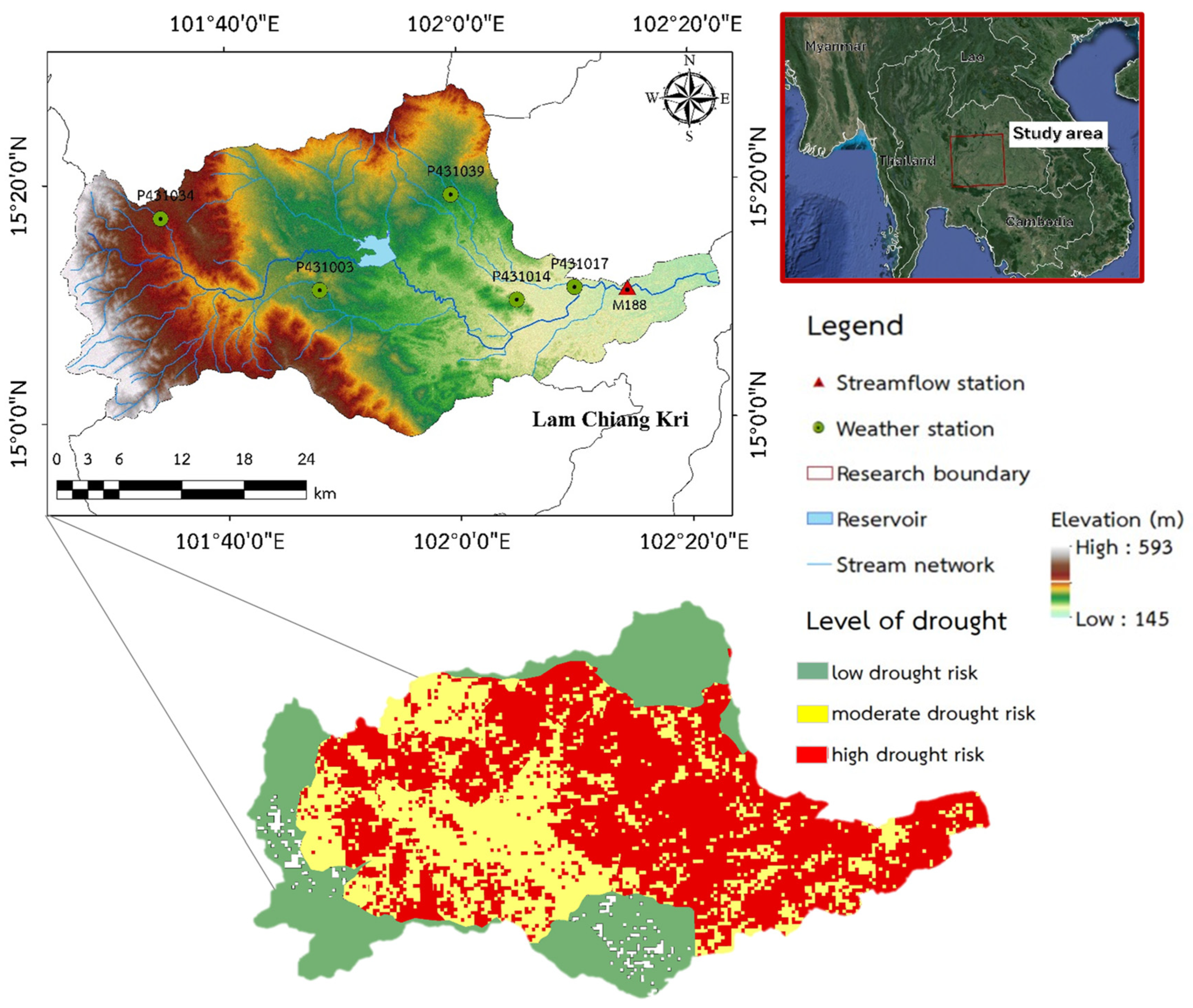
Figure 2.
A schematic diagram of the overall framework.
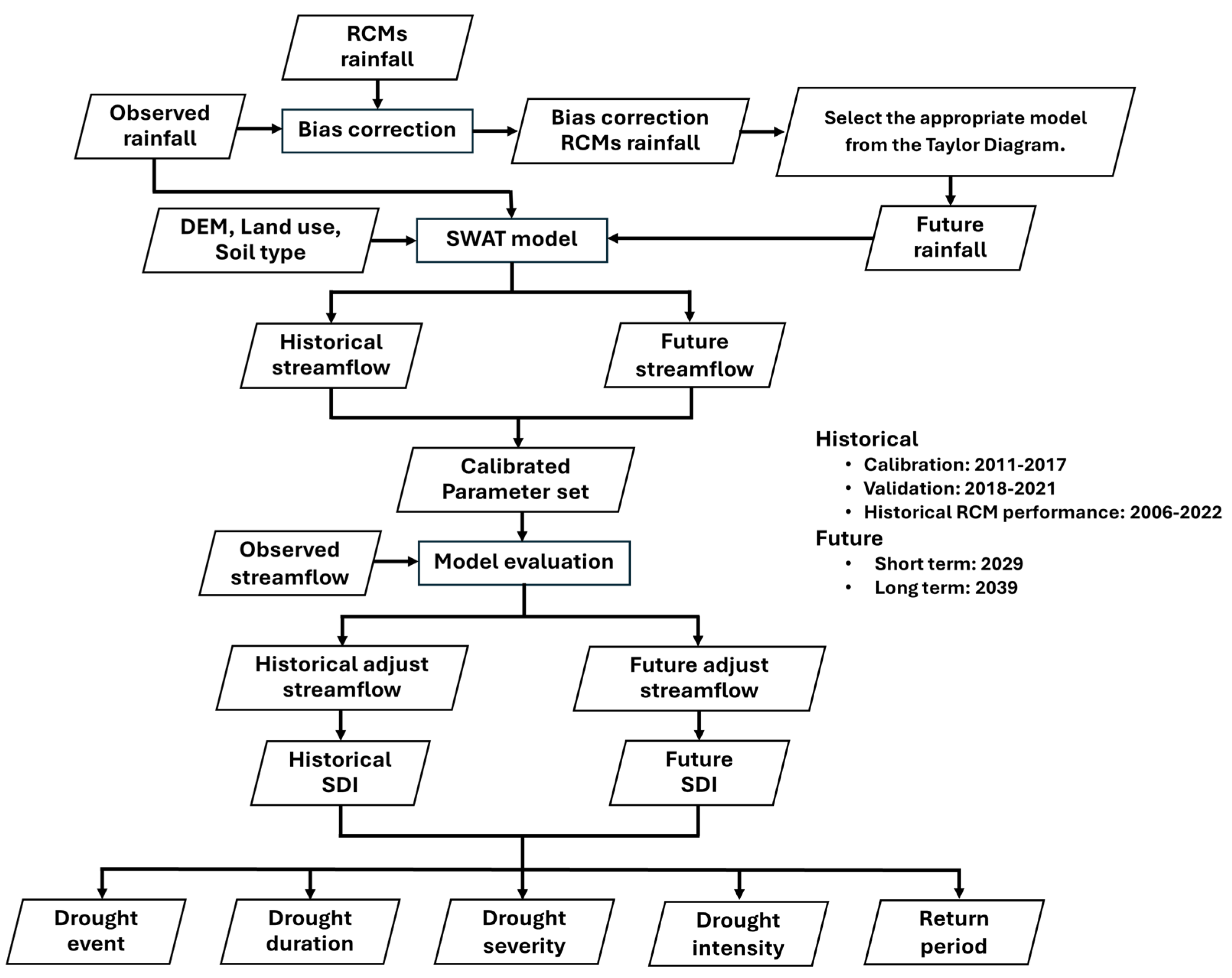
Figure 3.
A Theory of Runs illustration of a drought event and the drought indicators [45].
Figure 3.
A Theory of Runs illustration of a drought event and the drought indicators [45].
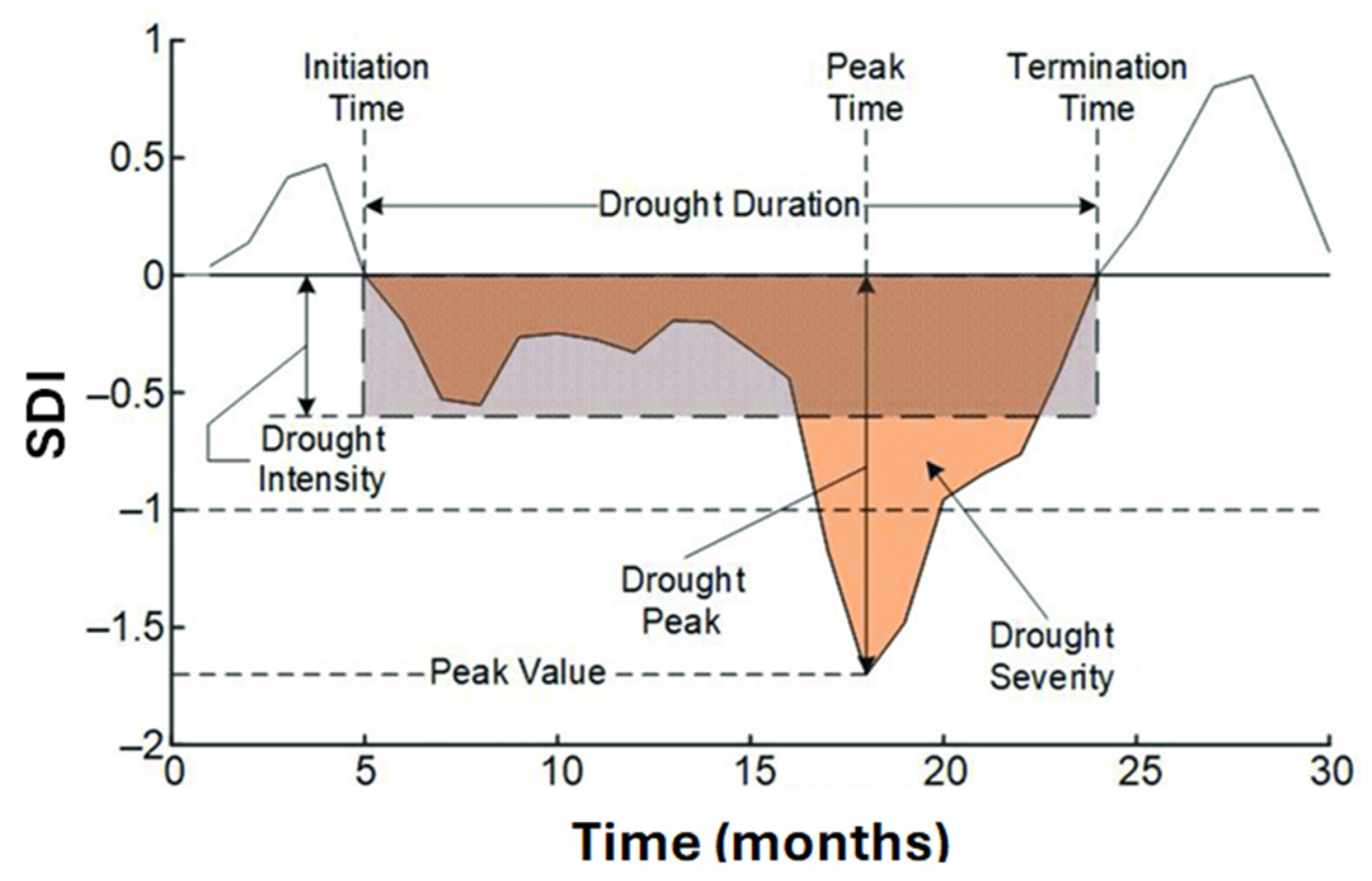
Figure 4.
The monthly simulated and observed streamflow correlations for M188 Station during the calibration (2010–2017) and validation (2018–2021) period. The calibration and validation periods are separated by horizontal dashed lines within the graphs.
Figure 4.
The monthly simulated and observed streamflow correlations for M188 Station during the calibration (2010–2017) and validation (2018–2021) period. The calibration and validation periods are separated by horizontal dashed lines within the graphs.
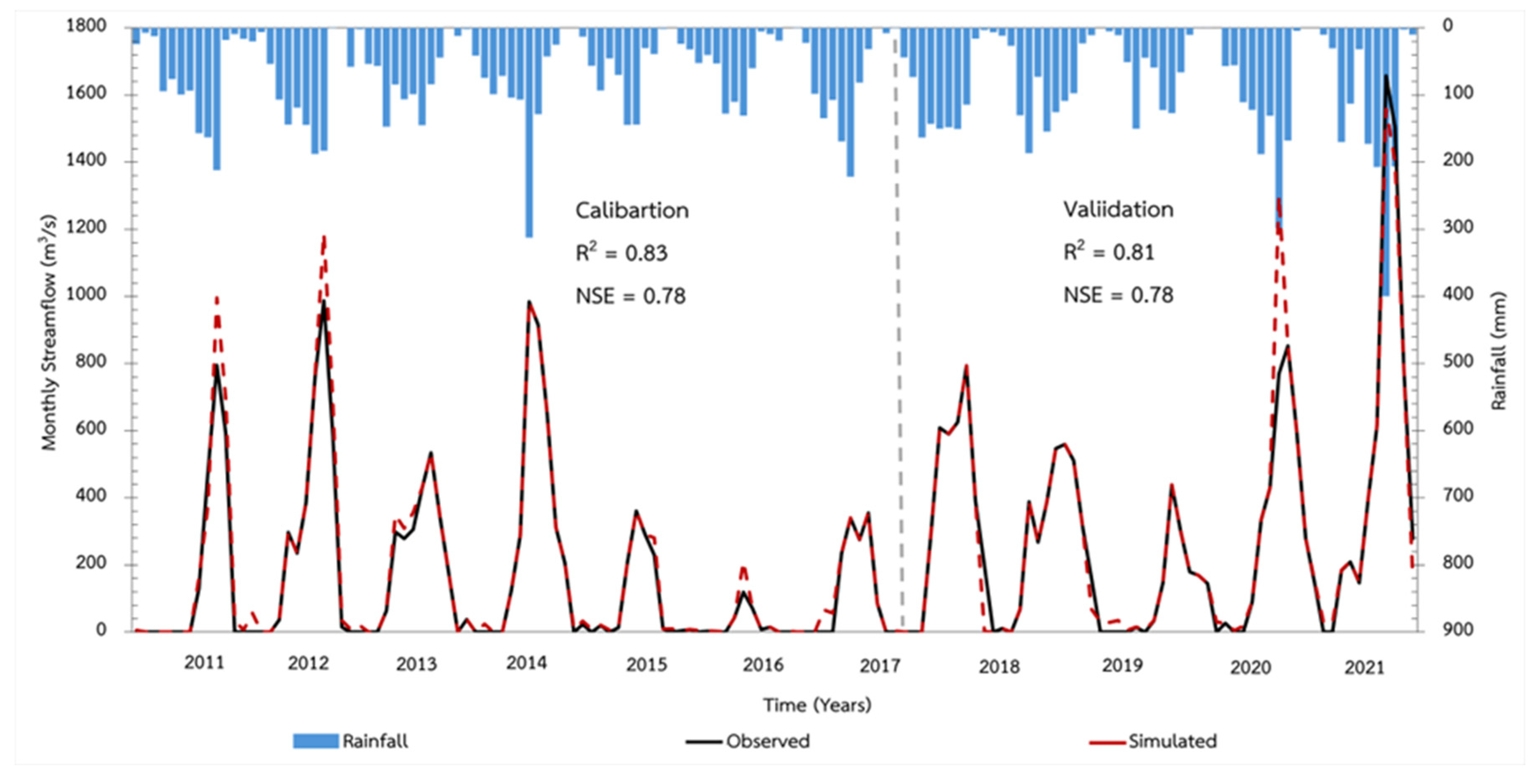
Figure 5.
The temporal variation in spatial averaged time series for the SDI over the LCKW at 3-, and 6-month time scales calculated based on the period of 2010–2022. A color scale moving from yellow to red represents mild, moderate, severe, and extreme drought categories, respectively.
Figure 5.
The temporal variation in spatial averaged time series for the SDI over the LCKW at 3-, and 6-month time scales calculated based on the period of 2010–2022. A color scale moving from yellow to red represents mild, moderate, severe, and extreme drought categories, respectively.
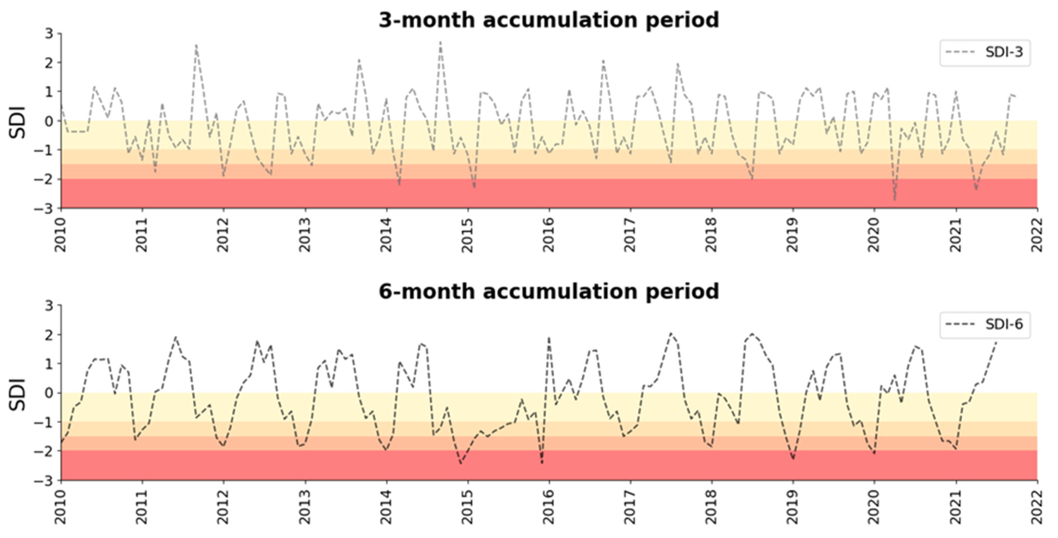
Figure 6.
The Taylor Diagram illustrates the suitability of different climate models for projecting rainfall in the LCKW.
Figure 6.
The Taylor Diagram illustrates the suitability of different climate models for projecting rainfall in the LCKW.
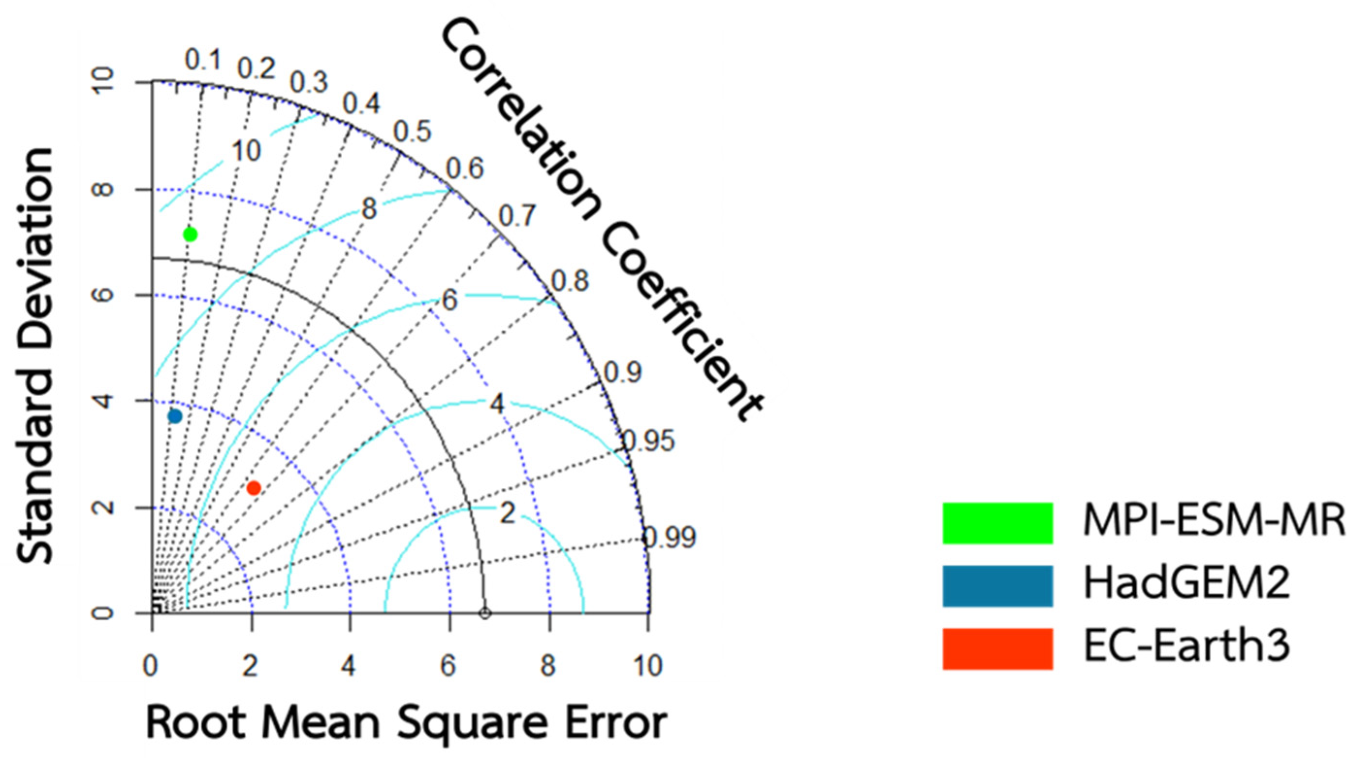
Figure 7.
Compare the streamflow during the baseline period (2004–2022) with projections for 2029 and 2039 under the future climate scenarios RCP4.5 and RCP8.5.
Figure 7.
Compare the streamflow during the baseline period (2004–2022) with projections for 2029 and 2039 under the future climate scenarios RCP4.5 and RCP8.5.
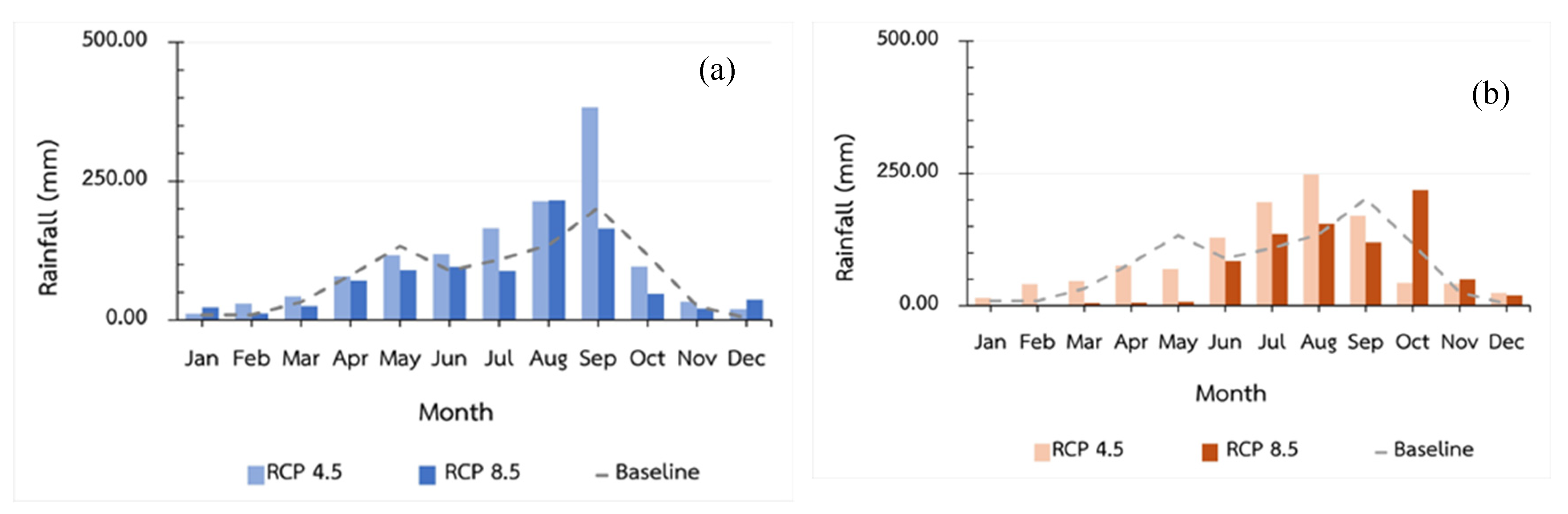
Figure 8.
Compare the streamflow during the baseline period (2010–2021) with projections for 2029 and 2039 under the future climate scenarios RCP4.5 and RCP8.5.
Figure 8.
Compare the streamflow during the baseline period (2010–2021) with projections for 2029 and 2039 under the future climate scenarios RCP4.5 and RCP8.5.
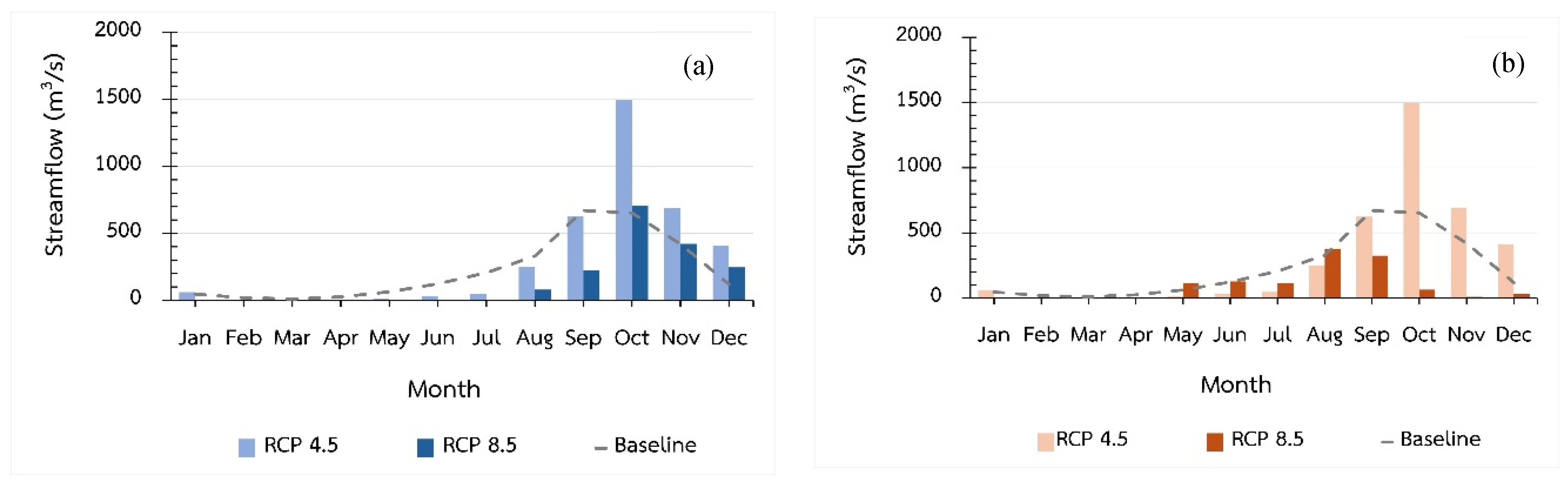
Figure 9.
Temporal variation of spatial averaged time series for SDI over LCKW at 3-, and 6-month time scales calculated based on Ec-Earth3 model. (a) 2029; (b) 2039. The color scale moving from yellow to red represents mild, moderate, severe, and extreme drought categories, respectively.
Figure 9.
Temporal variation of spatial averaged time series for SDI over LCKW at 3-, and 6-month time scales calculated based on Ec-Earth3 model. (a) 2029; (b) 2039. The color scale moving from yellow to red represents mild, moderate, severe, and extreme drought categories, respectively.
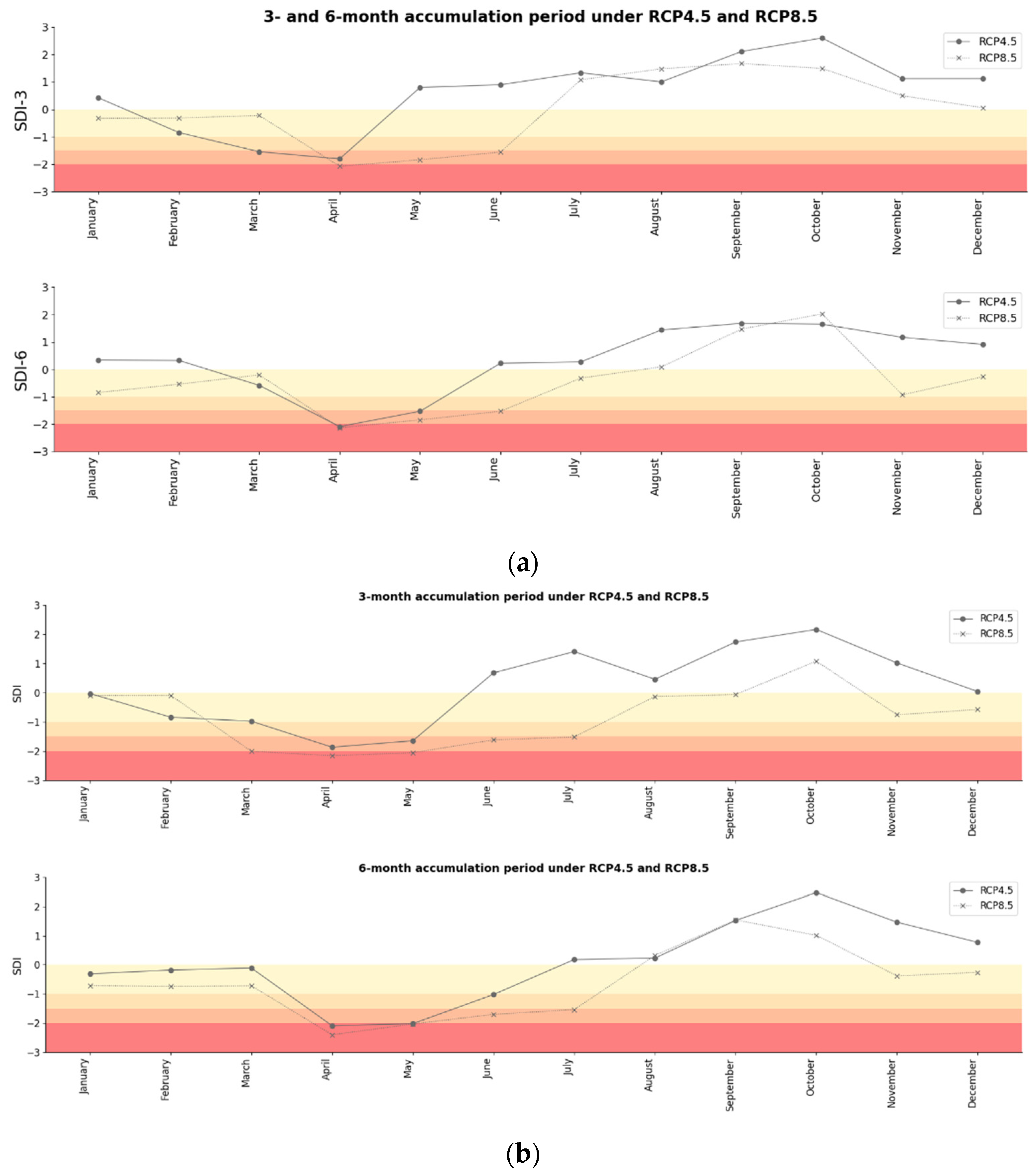
Figure 10.
The wavelet analysis shows the relationship between the amount of streamflow (m3/s), absolute SDI and return periods (a) reference period (b) RCP4.5 and (c) RCP8.5.
Figure 10.
The wavelet analysis shows the relationship between the amount of streamflow (m3/s), absolute SDI and return periods (a) reference period (b) RCP4.5 and (c) RCP8.5.
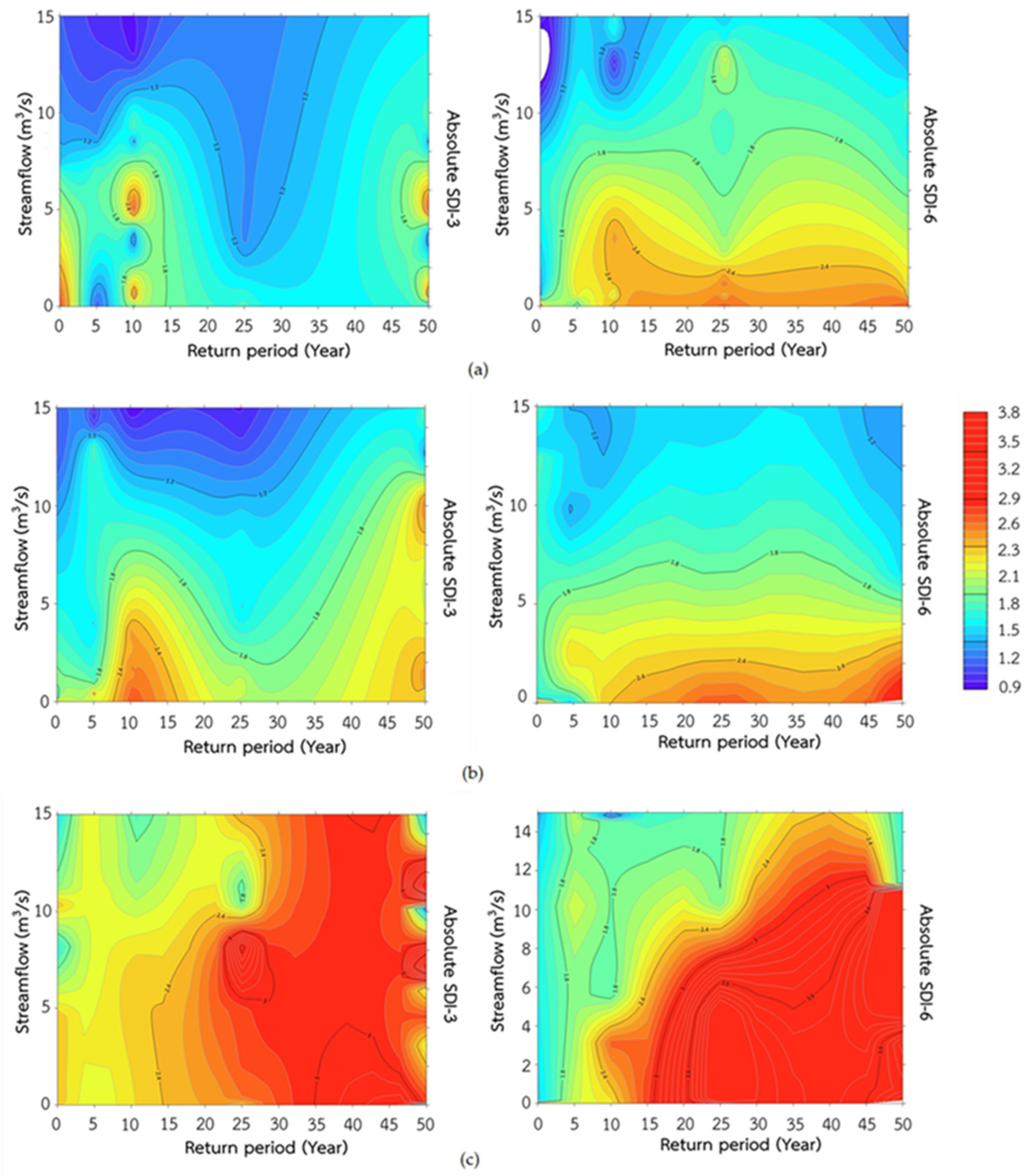

Table 1.
Classification of hydrological drought based on SDI [43].
Table 1.
Classification of hydrological drought based on SDI [43].
| State | Description | Range |
|---|---|---|
| 1 | No drought | 0 ≤ SDI |
| 2 | Mild drought | −1 ≤ SDI < 0 |
| 3 | Moderate drought | −1.5 ≤ SDI < −1 |
| 4 | Severe drought | −2 ≤ SDI < −1.5 |
| 5 | Extreme drought | SDI ≤ −2 |
Table 2.
Sensitive parameters in SWAT-CUP model at LCKW.
| Parameter | t-Stat | P-Value | Fit Value | Min Value | Max Value |
|---|---|---|---|---|---|
| 1: R__CN2.mgt | -5.48 | 0.01 | 40.395 | 35 | 100 |
| 2: R__SOL_AWC(..).sol | -2.84 | 0.04 | 0.343 | -0.2 | 0.4 |
| 3: R__ESCO.hru | 2.16 | 0.08 | 0.21525 | 0.1 | 0.35 |
| 4: V__GW_DELAY.gw | 1.82 | 0.14 | 155.5 | 0 | 500 |
| 5: R__SLSUBBSN.hru | -1.71 | 0.17 | 56.90 | 50 | 150 |
Table 3.
Statistical parameters of the SWAT model using SWAT-CUP.
| Statistic Parameters | Calibration (2011-2017) | Validation (2018-2021) | Total (2011-2021) |
|---|---|---|---|
| R2 | 0.83 | 0.81 | 0.82 |
| NSE | 0.78 | 0.78 | 0.78 |
| PBIAS | 12.0 | 28.04 | 20.02 |
| KGE | 0.64 | 0.46 | 0.55 |
Table 4.
Historical drought characteristics in the LCKW represented by the SDI for 3-, and 6- month accumulation periods.
Table 4.
Historical drought characteristics in the LCKW represented by the SDI for 3-, and 6- month accumulation periods.
| Hydrological Drought | ||
| SDI-3 | SDI-6 | |
| Average drought event (time/year) | 2.67 | 1.25 |
| Total number of drought events (times) | 32 | 15 |
| Maximum drought duration (months) | 23 | 36 |
| Maximum drought severity | -31.97 | --43.04 |
| Maximum drought intensity based on DI1 | -2.44 | -2.74 |
| Maximum drought intensity based on DI2 | -1.35 | -1.69 |
Table 5.
details future rainfall changes in the RCP4.5 and RCP8.5 scenarios for 2029 and 2039, compared to the baseline period of 2004-2022.
Table 5.
details future rainfall changes in the RCP4.5 and RCP8.5 scenarios for 2029 and 2039, compared to the baseline period of 2004-2022.
| Time | Baseline (2004-2022) |
RCP4.5 | RCP8.5 | ||
| (mm) | (mm) | % Change | (mm) | % Change | |
| 2029 | 947.64 | 1311.94 | 38.44 | 892.97 | -5.77 |
| 2039 | 947.64 | 1101.06 | 16.19 | 805.46 | -15.00 |
Table 6.
Compare the amount of streamflow in the baseline (2010 –2021) under future climate RCP4.5 and RCP8.5 scenario, both 2029 and 2039.
Table 6.
Compare the amount of streamflow in the baseline (2010 –2021) under future climate RCP4.5 and RCP8.5 scenario, both 2029 and 2039.
| Months | Baseline (m3/s) |
Future streamflow (m3/s) | ||||
| RCP4.5 | RCP8.5 | |||||
| 2029 | 2039 | 2029 | 2039 | |||
| observation | simulated | observation | simulated | observation | simulated | |
| January | 45.96 | 46.59 | 60.83 | 45.78 | 4.94 | 4.94 |
| February | 19.30 | 19.30 | 1.20 | 10.92 | 0.00 | 5.76 |
| March | 9.77 | 10.66 | 0.13 | 9.66 | 0.00 | 6.69 |
| April | 24.54 | 25.14 | 0.13 | 9.66 | 0.19 | 0.19 |
| May | 62.52 | 63.23 | 12.08 | 6.08 | 0.07 | 116.05 |
| June | 122.29 | 123.02 | 30.30 | 7.45 | 0.33 | 128.14 |
| July | 205.78 | 206.47 | 46.95 | 15.21 | 4.57 | 114.43 |
| August | 329.76 | 330.48 | 249.36 | 159.97 | 80.37 | 378.82 |
| September | 626.43 | 671.42 | 624.79 | 474.93 | 225.28 | 325.10 |
| October | 652.15 | 653.03 | 1,495.52 | 1,495.52 | 708.20 | 65.79 |
| November | 419.28 | 419.99 | 691.80 | 593.66 | 421.28 | 10.70 |
| December | 143.72 | 119.69 | 410.01 | 363.35 | 247.15 | 30.93 |
| Total Runoff | 2,661.51 | 2,689.02 | 3,623.09 | 3,192.18 | 1,692.38 | 1,187.54 |
| wet period (m3/s) | 2,442.76 | 2,492.78 | 3,150.93 | 2,762.47 | 1,440.29 | 1,139.21 |
| dry period (m3/s) | 218.74 | 196.24 | 472.17 | 429.71 | 252.09 | 48.33 |
| (%) percentage change | - | - | 34.74 | 18.71 | -37.06 | -55.84 |
Disclaimer/Publisher’s Note: The statements, opinions and data contained in all publications are solely those of the individual author(s) and contributor(s) and not of MDPI and/or the editor(s). MDPI and/or the editor(s) disclaim responsibility for any injury to people or property resulting from any ideas, methods, instructions or products referred to in the content. |
© 2024 by the authors. Licensee MDPI, Basel, Switzerland. This article is an open access article distributed under the terms and conditions of the Creative Commons Attribution (CC BY) license (http://creativecommons.org/licenses/by/4.0/).
Copyright: This open access article is published under a Creative Commons CC BY 4.0 license, which permit the free download, distribution, and reuse, provided that the author and preprint are cited in any reuse.


