
Submitted:
01 August 2024
Posted:
05 August 2024
You are already at the latest version
Abstract
The task of automatically and intelligently diagnosing faults in marine equipment is of great significance due to the numerous duties that shipboard professionals must handle. Incorporating automated and intelligent systems on ships allows for more efficient equipment monitoring and better decision-making. This approach has attracted considerable interest in both academia and industry because of its potential for economic savings and improved safety. Several fault diagnosis methods are documented in the literature, often involving mathematical and control theory models. However, due to the inherent complexity of some processes, not all characteristics are precisely known, making mathematical modeling highly challenging. As a result, fault diagnosis often depends on data or heuristic information. Fuzzy logic theory is particularly well-suited for processing this type of information. Therefore, this paper employs fuzzy models to diagnose faults in a marine pneumatic servo-actuated valve. The proposed fault diagnosis framework analyzes the discrepancy signals between the outputs of the fuzzy models and the actual process outputs. These discrepancies, known as residuals, help in detecting and isolating equipment faults. The fault isolation process uses an intelligent decision-making approach to determine the specific fault in the system. This method is applied to diagnose abrupt faults in a marine pneumatic servo-actuated valve.
Keywords:
intelligent fault diagnosis
; model-based fault diagnosis
; fuzzy modeling
; marine equipment
1. Introduction
The drive for higher quality and increased productivity has led to more complex technical processes, which in turn has raised the demand for safety and reliability, particularly in marine system production [16]. Historically, predictive maintenance was employed, where maintenance actions were based on equipment condition monitoring via sensors and degradation timelines. This approach was heavily dependent on human expertise and intervention [15,18]. With the growing complexity of technical processes, the probability of faults increases. Marine equipment features interconnected subsystems, so a small fault can cause a chain reaction, affecting related subsystems and magnifying the original fault [24]. Incorporating automatic supervision into control systems can detect and isolate faults early. Several fault diagnosis methods have been developed, with model-based fault diagnosis emerging in the early 1970s. This technique has garnered increasing attention for detecting faults in dynamic systems. Fault detection and isolation methods identify discrepancies between system outputs and model outputs, flagging these as faults. However, these discrepancies can also result from model-plant mismatches or noise in measurements, potentially leading to false fault detections. A good model of the monitored system can enhance diagnostic tool performance and reduce false alarms [22]. The residual, representing the inconsistency between system measurements and model signals, is critical in model-based fault diagnosis. Proper residual generation is essential to avoid losing fault information. There is a growing demand for effective fault diagnosis systems to improve the safety and reliability of marine systems [1]. Given the variety of onboard equipment, diagnosing faults in a pneumatic servo-actuated valve is crucial to prevent faults and serious consequences. Detecting and isolating faults promptly can prevent costly damage and loss of efficiency and productivity.
This paper proposes a model-based fault diagnosis architecture that synergistically combines fuzzy modeling with an intelligent decision-making approach. Fault diagnosis involves fault detection and fault isolation. First, fuzzy models for normal operation and each fault are identified, predicting system outputs from process inputs and outputs, and directly deriving a fuzzy model from the data. Detection involves computing the residual by comparing real data with the system’s fuzzy model during normal operation. When a fault is detected, each faulty model output is compared to the actual process outputs. Once detected, the fault must be isolated. Residuals from each fault model are evaluated using an intelligent decision-making approach to isolate the fault.
This paper is structured as follows: Section 2 reviews literature on fault diagnosis and redundancy methods. Section 3 presents fuzzy modeling. Section 4 outlines the proposed intelligent fault diagnosis approach. Section 5 discusses the application to marine equipment. Section 6 details the experiments and results of applying the proposed fault diagnosis method. Finally, Section 7 offers conclusions.
2. Fault Diagnosis
Numerous Fault Detection and Isolation (FDI) approaches have been developed in recent years across various installations. One of the initial methods was the failure detection filter for linear systems [3]. This was followed by various techniques, such as identification methods for detecting faults in jet engines [19] and correlation methods for leak detection [20]. Isermann introduced methods for process fault detection based on modeling parameters and state estimations [10]. Model-based fault detection and diagnosis techniques for chemical processes were detailed in [9]. In the frequency domain, FDI is performed using frequency spectra to isolate faults [5]. Other approaches include residual generators, which can be based on either physical or hardware redundancy methods, or analytical or functional redundancy methods [4]. More recently, transfer learning has been applied to Marine Diesel Engines [7], and adaptive neural networks have been used for fault diagnosis in ship power equipment [27]. A hierarchical method combining domain knowledge of ship engines with advanced data analysis techniques was proposed in [26]. Fault diagnosis has gained widespread acceptance in the academic community and is extensively applied in maritime environments, particularly on ships.
The following section introduces the technique used in this paper, which is based on redundancy-based fault diagnosis.
2.1. Fault Diagnosis Redundancy Methods
When redundant systems are used in fault diagnosis, their reliability increases. Consequently, a causality-based fault diagnosis method has been proposed for systems that utilize redundancy [25]. Traditionally, fault diagnosis has relied on hardware redundancy, which involves using multiple sensors, actuators, and components to measure and control a variable. However, this method has drawbacks, such as increased equipment and maintenance costs and the need for additional space [11]. These limitations emphasize the need for alternative, more cost-effective methods.
Analytical or functional redundancy methods are promising alternatives. These methods use redundant analytical relationships among various measured variables in the monitored system [4,12]. These variables are actual measurements compared with estimated values generated by a mathematical model of the system. In an analytical redundancy scheme, the difference between these values, known as the residual or symptom signal, should be zero during normal operation and non-zero when a fault occurs. This property helps identify faults. Examples of residual generators include the Kalman filter, Luenberger observers, state and output observers, and parity relations [4]. Model-based FDI, which involves detecting and isolating faults by extracting features from measured signals, has been applied in various fields, including marine diesel engines [14]. The first step in model-based FDI is generating residuals from the system’s inputs and outputs by comparing measured outputs (y) with estimated outputs (ŷ). A mechanism then evaluates the residuals by checking if they exceed a reference value, indicating a fault. For simple faults detectable by a single measurement, a conventional threshold check may be enough [4]. Figure 1 illustrates the fault detection approach based on residual analysis. The accuracy of the model representing the process is crucial for effective model-based fault detection. Without a reliable model, accurate fault diagnosis is impossible. The second step in model-based fault diagnosis involves an intelligent decision-making approach. Multiple residuals are designed, each sensitive to specific faults in different system locations. Once a residual exceeds its threshold, it isolates the fault. Residuals can be evaluated using statistical tests [13]. However, the inherent uncertainty in fully understanding the monitored process complicates this approach. While reducing sensitivity to modeling uncertainty can aid in fault diagnosis, it might also decrease sensitivity to actual faults [4,6]. Thus, the primary challenge of model-based fault diagnosis is dealing with the inevitable modeling uncertainty in real industrial systems. Various approaches to fault diagnosis in marine equipment, including model-based, data-driven, knowledge-based, and hybrid methods, are discussed in [17], along with perspectives on future directions in this field.
3. Fuzzy Modeling
Expert systems leverage inference techniques to tackle complex problems that typically require specialized human expertise. They offer several benefits, including quick response times, increased reliability, cost efficiency, and adaptability. Due to these advantages, expert systems have found applications across various fields. This paper introduces an expert system grounded in fuzzy logic principles through fuzzy modeling. Fuzzy modeling usually involves encoding expert knowledge, often articulated in verbal form, into a series of if–then rules, thereby forming a model structure. This structure’s parameters can be adjusted using input-output data. In cases where prior system knowledge is lacking, a fuzzy model can be entirely derived from system measurements. The fault diagnosis approach discussed here utilizes fuzzy models. Specifically, we will explore data-driven modeling based on fuzzy clustering techniques [21].
Now, let’s focus on rule-based models of the Takagi-Sugeno (TS) type [23]. These models consist of fuzzy rules, each representing a local input-output relationship, typically expressed in an affine form.
where i = 1,2, …, K. Here Ri is the ith rule, x =[x1,…,xn]Tis the antecedent vector, Ai1,…,Ain are fuzzy sets defined in the antecedent space, and yi is the output of the rule. The parameter K denotes the total number of rules in the rule base. The overall output of the model, , is obtained by calculating the weighted average of the rule consequents:
the degree of activation of the ith rule, denoted as , is defined by the formula = , where i = 1,2,…, K . Here, ℝ → [0,1] represents the membership function of the fuzzy set Aij in the antecedent of the rule Ri.
Ri: If x1 is Ai1 and … and xn is Ain then yi = aix+bi
To identify the model (2), we first construct the regression matrix X and the output vector y using the available data XT= [x1,…,xN]; yT= [y1,…,yN]. In this context, N ≫n, representing the number of samples used for model identification.
The number of rules, K, the antecedent fuzzy sets, Aij, and the consequent parameters, ai, biare determined through fuzzy clustering applied to the product space X Y [2]. The data set Z to be clustered is represented as ZT=[X,y]. With Z and an estimated number of clusters K, the Gustafson-Kessel fuzzy clustering algorithm [8] is used to compute the fuzzy partition matrix U.
The fuzzy sets in the antecedent of the rules are derived from the partition matrix U, where each ikth element μikϵ [0,1] , indicates the membership degree of the data object zkin cluster i. One-dimensional fuzzy sets Aij are obtained by projecting the multidimensional fuzzy sets defined in the ith row of the partition matrix onto the input variable space xj.
The consequent parameters for each rule are derived using a weighted ordinary least-square estimate. Let where Xerepresents the matrix [X;1] and Wiis a diagonal matrix in ℝNXN with the degree of activation, βi(xk), as its kth diagonal element. Provided that the columns of Xeare linearly independent and βi(xk) > 0 for 1 ≤ k ≤ N, the weighted least squares solution of y = Xeq +ε is given by:
4. Proposed Intelligent Fault Diagnosis
This paper introduces a model-based architecture for fault diagnosis that involves both fault detection and fault isolation. The process for these steps is outlined below. The proposed method employs fuzzy modeling, with models derived directly from the available process data. Notably, this approach allows for the use of any type of model—whether white-box or black-box, such as fuzzy or neural networks—since the architecture relies solely on the model outputs.
In this technique, a fuzzy model represents the process during normal operation, and separate fuzzy models are used for each fault that needs to be isolated. The fault detection fuzzy model is developed using data from the process without faults. Faults are detected when the residual, calculated by comparing the process outputs with those of the fuzzy mode, exceeds a predefined threshold. For fault isolation, individual fuzzy models are created for each potential fault using data from the process when faults are present. A fault is isolated when the residual, obtained by comparing the process outputs with the outputs of these fault-specific fuzzy models, exceeds a certain threshold. Assuming a process operates with n possible faults, the fault detection and isolation system described in this paper is illustrated in Figure 2. The system’s multidimensional input is fed into both the process and an observer model during normal operation. The residual vector, denoted as ∈, is defined as:
∈=𝒚−𝒚̂
In this system, y represents the actual system output, while ŷ is the model’s predicted output under normal conditions. A fault is detected when any component of ∈ exceeds a specific threshold δ . Once a fault is detected, n models are activated, one for each potential fault, and n residual vectors are calculated.
In the fault diagnosis framework illustrated in Figure 2, fault isolation is achieved by evaluating the residuals from each of the n models, corresponding to each fault. At each time step k , a residual ∈i is calculated for each fault:
the variable ŷi represents the output of the observer for fault i, where i ranges from 1 to n. It is important to note that the residual ∈i is a vector with a dimension of m, corresponding to the number of outputs.
∈𝑖(𝑘)=𝒚𝒊 − 𝒚̂𝒊
Next, we will outline the intelligent decision-making process for fault isolation. Fault detection triggers the activation of models corresponding to each fault, as illustrated in Figure 2. Once residuals for each fault model are obtained, they are aggregated over a time range from instant k to instant k-p. The value of p should be chosen based on the variability of the system’s outputs under analysis. Specifically, p may need to be increased if output variability is high and decreased if it is low. Using a time range from instant k to instant k-5 helps the method accommodate temporary fluctuations in fault model outputs that might occur without indicating actual faults. Given that a fault model may have multiple outputs, this paper suggests calculating the maximum aggregate values of the residuals for these outputs. This approach provides an overall aggregate residual value for each fault model. To determine the existence of multiple faults, we assess the total residuals for each fault model. The fault is isolated by selecting the model with the lowest total residual value.
5. Marine Equipment
The pneumatic servo-actuated valve used for marine control, illustrated in Figure 3, serves as the testbed for the fault diagnosis approach proposed in this paper. This actuator comprises three primary components: the control valve (V), the pneumatic servomotor (S), and the positioner (P). Each of these components includes several subcomponents: the positioner supply air pressure (PSP), the air pressure transmitter (PT), the volume flow rate transmitter (FT), the temperature transmitter (TT), the rod position transmitter (ZT), the electro-pneumatic converter (E/P), and the controller output (CVI). Analysis of these variables indicates that the most critical factors for fault diagnosis are the flow process (PV) and the rod displacement of the servomotor (X), which are the primary outputs considered in the model.
6. Experiments and Results
6.1. Process Data
The analysis of the process variables revealed that the key input variables for modeling are input pressure, output pressure, temperature, and reference. The primary output variables are flow and rod displacement. Figure 4 displays process data in the absence of faults.
Data process with fault F1 are shown in Figure 5.
Data process with fault F2 are shown in Figure 6.
Data process with fault F3 are shown in Figure 7.
6.2. Models Identification
The weighted least squares solution presented in (3) was calculated for each of the output variables across models with and without faults (F1, F2, and F3). The matrices below display the results for the output flow (PV) and output rod displacement (X). For the fault-free process, the output flow (PV) is as follows:
For the fault-free process, the output rod displacement (X) is as follows:
For the process with fault F1, the output flow (PV) is:
For the process with fault F1, the output rod displacement (X) is:
For the process with fault F2, the output flow (PV) is:
For the process with fault F2, the output rod displacement (X) is:
For the process with fault F3, the output flow (PV) is:
For the process with fault F3, the output rod displacement (X) is:
6.3. Results
The FDI method introduced in this paper, illustrated in Figure 2, was used to identify and isolate sudden faults in the pneumatic servo-actuated valve. Among the potential faults, three were specifically analyzed: F1, F2, and F3. Descriptions of these faults can be found in Table 1.
Table 2 shows the results obtained when different input faults occur in the system. Each row in Table 2 corresponds to a specific fault simulated, while each column represents the fault model used for isolation. The residuals for the faults considered are highlighted in bold. The fault diagnosis approach proposed in this paper successfully detects and isolates all three faults. The bold values in Table 2 represent the smallest residuals for their respective faults, indicating correct isolation.
The following figures illustrate the effectiveness of the fault detection and isolation method introduced in this paper. In Figure 8, you can see the residuals used for fault detection alongside the detection time. The residual for the flow output is significantly high and exceeds the set threshold, indicating that a fault has occurred. This conclusion is validated because the fault diagnosis technique was applied to data representing the process behavior with fault F1. The threshold is established through a method that integrates both learning from and understanding of the process behavior.
After detecting the fault, the second stage of the fault diagnosis process begins, as illustrated in Figure 2. In this stage, fault isolation is performed. Figure 9 presents the results obtained when the fault diagnosis method uses data from the process exhibiting fault F1. The residuals from the model for fault F1 are nearly zero, suggesting that fault F1 has been accurately isolated. In contrast, the residuals for the models of faults F2 and F3 are significantly different from zero, indicating that these faults are not present.
Figure 10 displays the results for the process behavior with fault F2. The residuals from the fault F2 model are nearly zero, demonstrating effective isolation of this fault. Conversely, the residuals for the F1 and F3 fault models are substantially larger, confirming that neither fault F1 nor fault F3 is present.
6. Conclusions
This paper presents a fault diagnosis system that utilizes fuzzy modeling combined with an intelligent decision-making approach to identify and address faults. The system integrates fuzzy models for both detecting and isolating faults. Specifically, the fault detection model is developed using data from the process when it is fault-free, while the fault isolation models are based on data from processes with faults. Fault detection and isolation rely on residual analysis. An intelligent decision-making strategy is employed to perform fault isolation by evaluating the residuals from each fuzzy fault model. The proposed architecture was applied to a pneumatic servo-actuated marine valve, demonstrating its capability to detect and isolate three distinct faults, despite the challenges introduced by noisy data.
Future work will focus on expanding this fault diagnosis and isolation (FDI) framework to accommodate a broader range of faults, including more complex types. Additionally, research will aim to develop intelligent systems for determining optimal threshold values and selecting the appropriate time instants for residual analysis. The methodology will also be integrated into fault-tolerant control systems.
References
- Aslam, S., Michaelides, M.P., and Herodotou, H. Internet of ships: A survey on architectures, emerging applications, and challenges. IEEE Internet of Things Journal. 2020, vol. 7, no. 10, p. 9714-9727. [Accessed: 24 April 2024]. [CrossRef]
- Babuška, R. Fuzzy Modeling for Control. Boston, MA: Kluwer Academic Publishers, 1998. ISBN 9789401148689.
- Beard, R. V. Failure accomodation in linear system through self-reorganization. Doctoral thesis, MIT. Boston, MA: Massachusetts Institute of Technology, 1971. [Accessed: 24 April 2024]. Available at: https://dspace.mit.edu/handle/1721.1/16415.
- Chen, R. and R. Patton. Robust model-based fault diagnosis for dynamic systems. Boston, MA: Kluwer Academic Publishers, 1999. ISBN 978079238411-3.
- Ding, X., and Frank, P. M. Fault detection via factorization approach [online]. System and Control Letters. 2000, vol.14, no. 5, p. 431–436. [Accessed: 24 April 2024]. Available at: https://doi.org/10.1016/0167-6911(90)90094-B.
- Gertler, J. Fault detection and diagnosis in engineering systems. New York: Marcel Dekker, 1998. ISBN 0824794273.
- Guo, Yu and Zhang, Jundong. Fault diagnosis of marine diesel engines under partial set and cross working conditions based on transfer learning [online]. J. Mar.Sci. Eng. 2023, vol. 11, no. 8, p. 1527. [Accessed: 24 April 2024]. Available at: https://doi.org/10.3390/jmse11081527.
- Gustafson, D.E. and W.C. Kessel. Fuzzy clustering with a fuzzy covariance matrix [online]. In: Proc. Of the 18th IEEE Conference on Decision and Control. San Diego, CA,: IEEE, 1979, p. 761–766. [Accessed: 24 April 2024]. Available at: 10.1109/CDC.1978.268028.
- Himmelblau, D. M. Fault diagnosis in chemical and petrochemical processes. Amsterdam: Elsevier, 1978. ISBN 9780444417473.
- Isermann, R. Process fault detection based on modelling and estimation methods: A survey [online]. Automatica 1984, vol. 20, no. 4, p. 387–404. [Accessed: 24 April 2024]. Available at: https://doi.org/10.1016/0005-1098(84)90098-0.
- Isermann, R., and Ballé, P. Trends in the application of model-based fault detection and diagnosis of technical processes [online]. Control Engineering Practice. 1997, vol. 5, no. 5, p. 709–719. [Accessed: 24 April 2024]. Available at: https://doi.org/10.1016/S0967-0661(97)00053-1.
- Kinnaert, M. Fault diagnosis based on analytical models for linear and nonlinear systems – A tutorial [online]. In: Preprints of the Fifth IFAC symposium on fault detection, supervision and safety for technical processes, SAFEPROCESS’2003, pp. 37–50. Washington, USA: Elsevier, 2003. [Accessed: 24 April 2024]. Available at: https://doi.org/10.1016/S1474-6670(17)36468-6.
- Kinnaert, M., Vrancic, D., Denolin, E., Juricic, D., and Petrovcic, J. Model-based fault detection and isolation for a gas–liquid separation unit [online]. Control Engineering Practice. 2000, vol. 8, no. 11, p. 1273–1283. [Accessed: 24 April 2024]. Available at: https://doi.org/10.1016/S0967-0661(00)00064-2.
- Kougiatsos N., Negenborn R., Reppa V. Distributed model-based sensor fault diagnosis of marine fuel engines [online]. IFAC-PapersOnLine, 2022, vol. 55, no. 6, p. 347-353. [Accessed: 24 April 2024]. Available at: https://doi.org/10.1016/j.ifacol.2022.07.153.
- Lazakis, I., Gkerekos C., and Theotokatos G. Investigating an SVM-driven, one-class approach to estimating ship systems condition [online]. Ships and Offshore Structures. 2018, vol. 14, no. 5, p. 432-441. [Accessed: 24 April 2024]. Available at: https://doi.org/10.1080/17445302.2018.1500189.
- Lazakis, I., Raptodimos Y., Varelas T. Predicting ship machinery system condition through analytical reliability tools and artificial neural networks [online]. Ocean Engineering. 2018, vol. 152, p. 404-415. [Accessed: 24 April 2024]. Available at: https://doi.org/10.1016/j.oceaneng.2017.11.017.
- Lv Y., Yang X., Li Y., Liu J., Li S. Fault detection and diagnosis of marine diesel engines: A systematic review [online]. Ocean Engineering. 2024, vol. 294, p. 116798. [Accessed: 24 April 2024]. Available at: https://doi.org/10.1016/j.oceaneng.2024.116798.
- Raptodimos Y. and Lazakis I. Using artificial neural network-self-organising map for data clustering of marine engine condition monitoring applications [online]. Ships and Offshore Structures, 2018, vol. 13, no. 6, p. 649-656. [Accessed: 24 April 2024]. Available at: https://doi.org/10.1080/17445302.2018.1443694.
- Rault, A., Richalet, A., Barbot, A., & Sergenton, J. P. Identification and modelling of a jet engine. In: IFAC symposium of digital simulation of continuous processes, Gejor. 1971.
- Siebert, H., & Isermann, R. Fault diagnosis via on-line correlation analysis. Technical report, 25-3, VDI-VDE, 1976.
- Sousa, J.M. and U. Kaymak. Fuzzy Decision Making in Modeling and Control. Singapore: World Scientific Pub. Co., 2002.
- Sun, X., Tan, J., Wen, Y., and Feng, C. Rolling bearing fault diagnosis method based on data-driven random fuzzy evidence acquisition and Dempster–Shafer evidence theory [online]. Advances in Mechanical Engineering, 2016, vol. 8, no. 1, p. 1–8. [Accessed: 24 April 2024]. Available at: https://doi.org/10.1177/1687814015624834.
- Takagi, T. and M. Sugeno. Fuzzy identification of systems and its applications to modelling and control [online]. IEEE Transactions on Systems, Man, and Cybernetics. 1985, vol. 15, no. 1, p. 116–132. [Accessed: 24 April 2024]. Available at: https://doi.org/10.1109/TSMC.1985.6313399.
- Tan Y., Zhang J., Tian H., Jiang D., Guo L., Wang G., and Lin Y. Multi-label classification for simultaneous fault diagnosis of marine machinery: A comparative study[online]. Ocean Engineering, 2021, vol. 239, p. 109723. [Accessed: 24 April 2024]. Available at: https://doi.org/10.1016/j.oceaneng.2021.109723.
- Yin Y, Xu F, Pang B. Online intelligent fault diagnosis of redundant sensors in PWR based on artificial neural network [online]. Front. Energy Res., 20 September 2022. Sec. Nuclear Energy. 2022, Vol. 10. [Accessed: 24 April 2024]. Available at: https://www.frontiersin.org/articles/10.3389/fenrg.2022.1011362/full.
- Young, J.K., Yoojeong, N, Min-S. J., Sunyoung, P., Ju-Tae, K. Hierarchical level fault detection and diagnosis of ship engine systems [online]. Expert Systems with Applications. 2023, vol. 213, Part A, p. 118814. [Accessed: 24 April 2024]. Available at: https://doi.org/10.1016/j.eswa.2022.118814.
- Zhang, D. Fault diagnosis of ship power equipment based on adaptive neural network [online]. International Journal of Emerging Electric Power Systems, 2022, vol. 23, no. 6, pp. 779-791. [Accessed: 24 April 2024]. Available at: https://doi.org/10.1515/ijeeps-2022-0103.
Figure 1.
Fault detection approach.
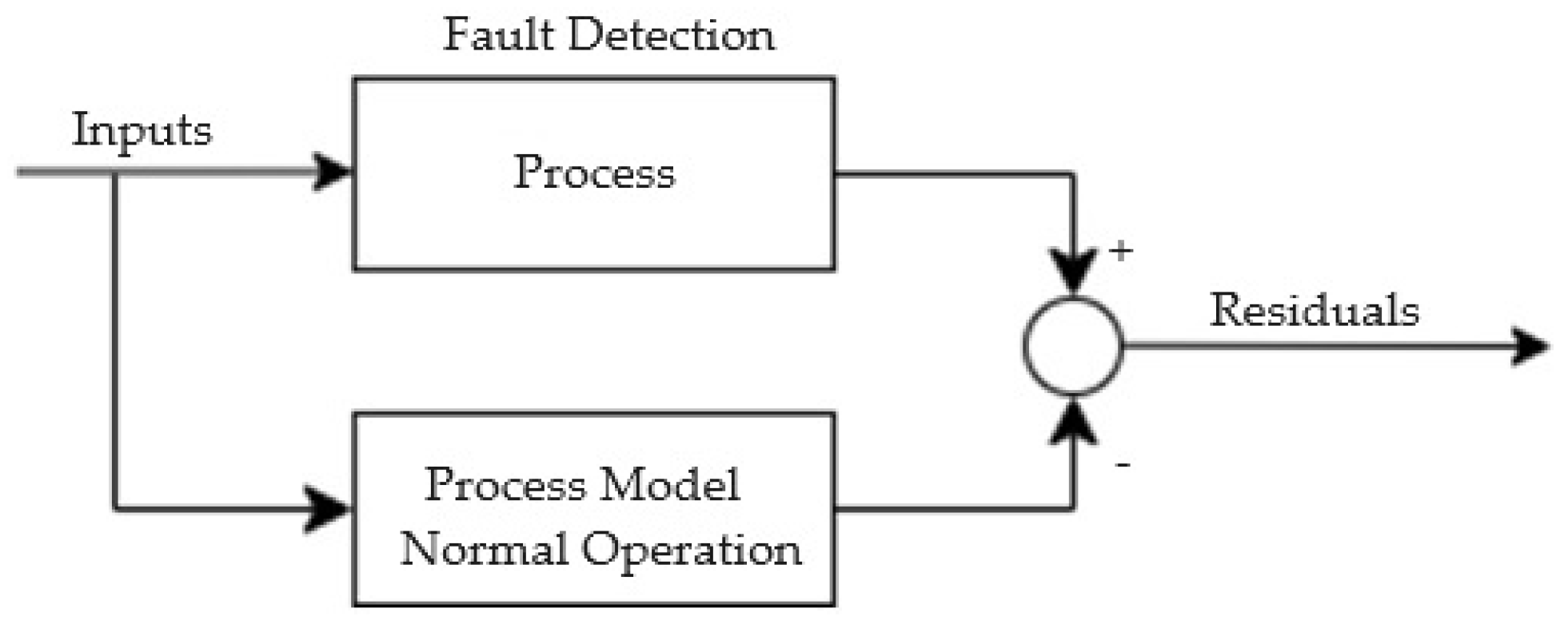
Figure 2.
Fault detection and isolation approach.
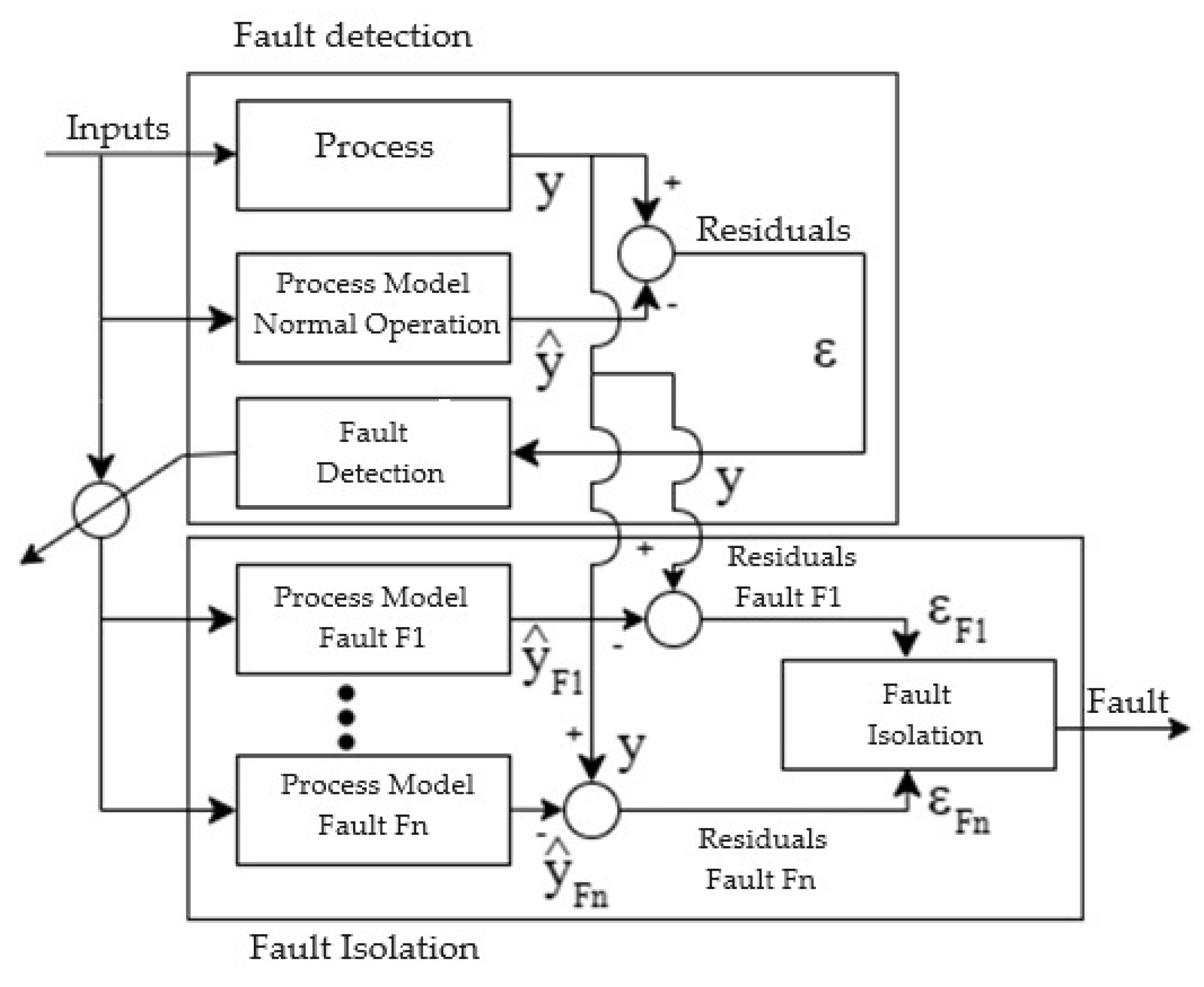
Figure 3.
Diagram of the pneumatic servo-actuated valve.
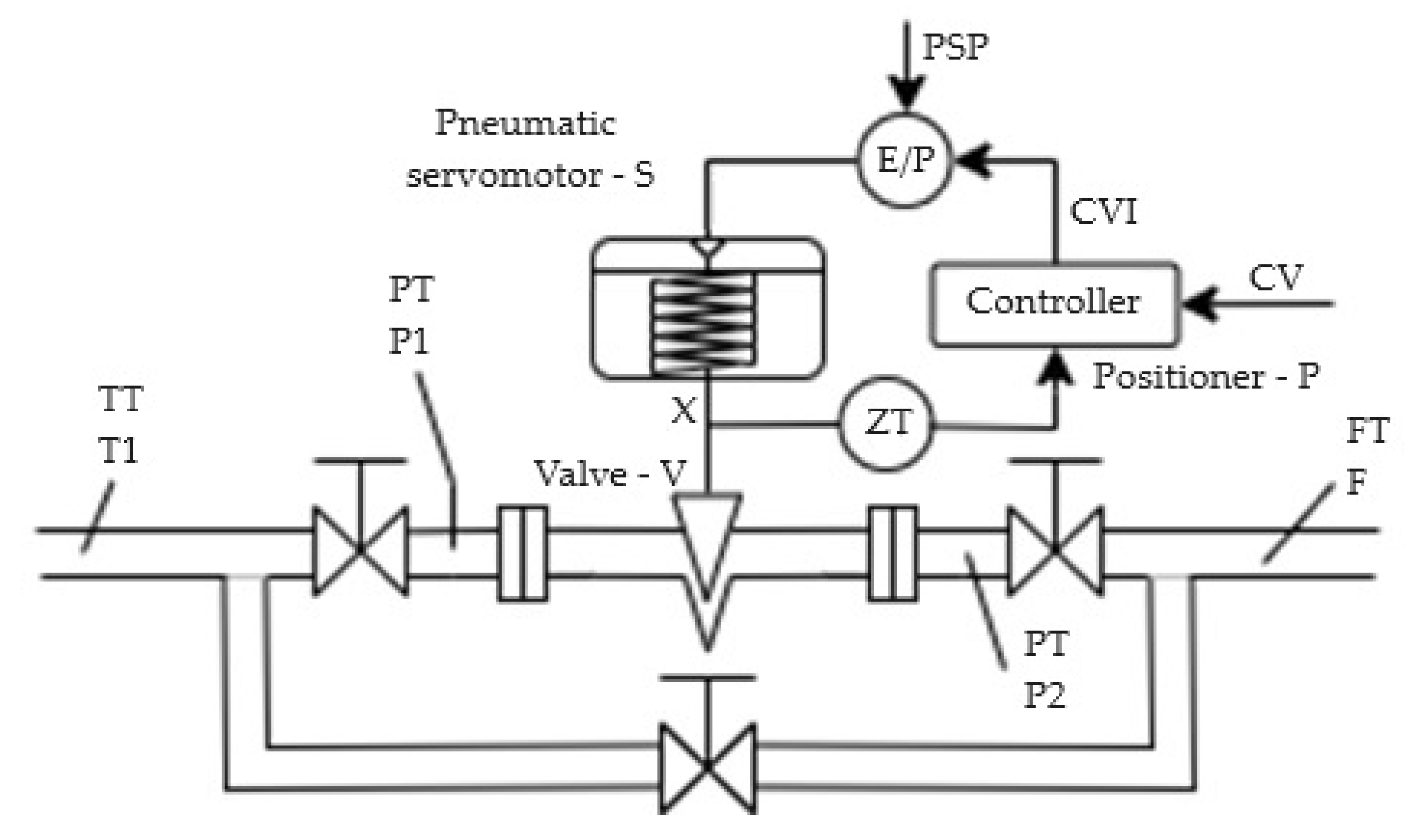
Figure 4.
Process data without fault.
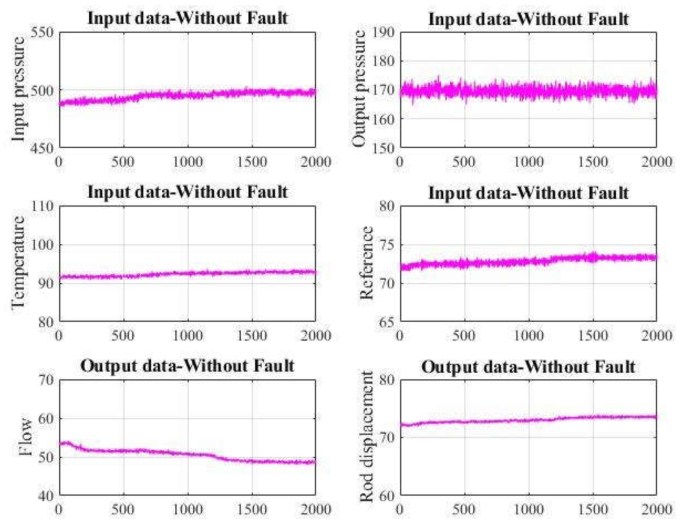
Figure 5.
Process data with fault F1.
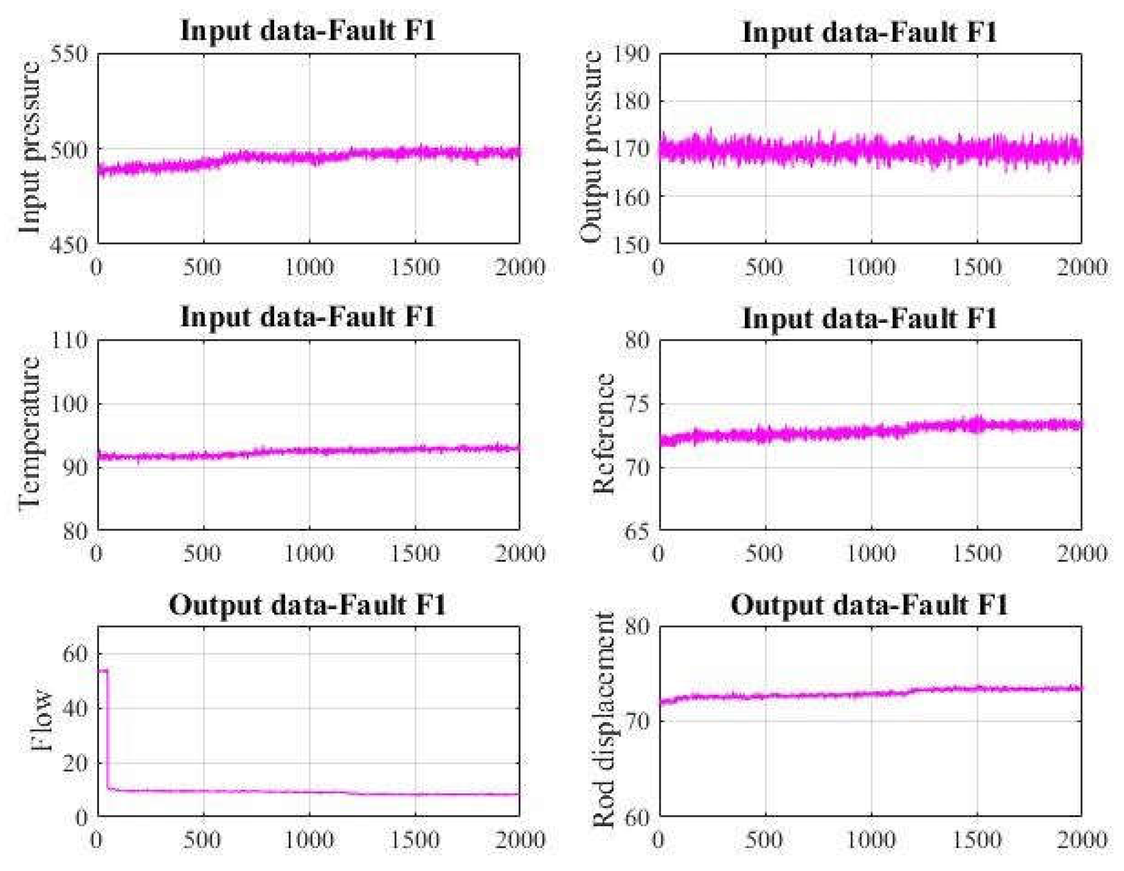
Figure 6.
Process data with fault F2.
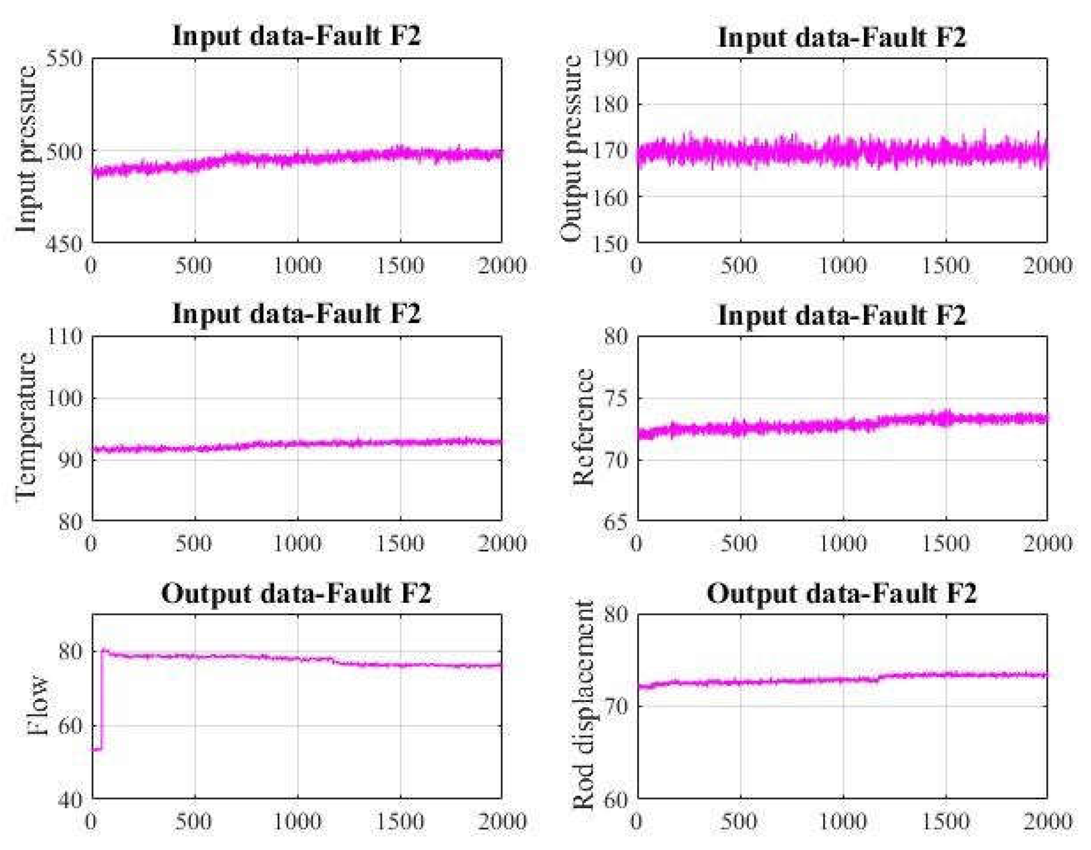
Figure 7.
Process data with fault F3.
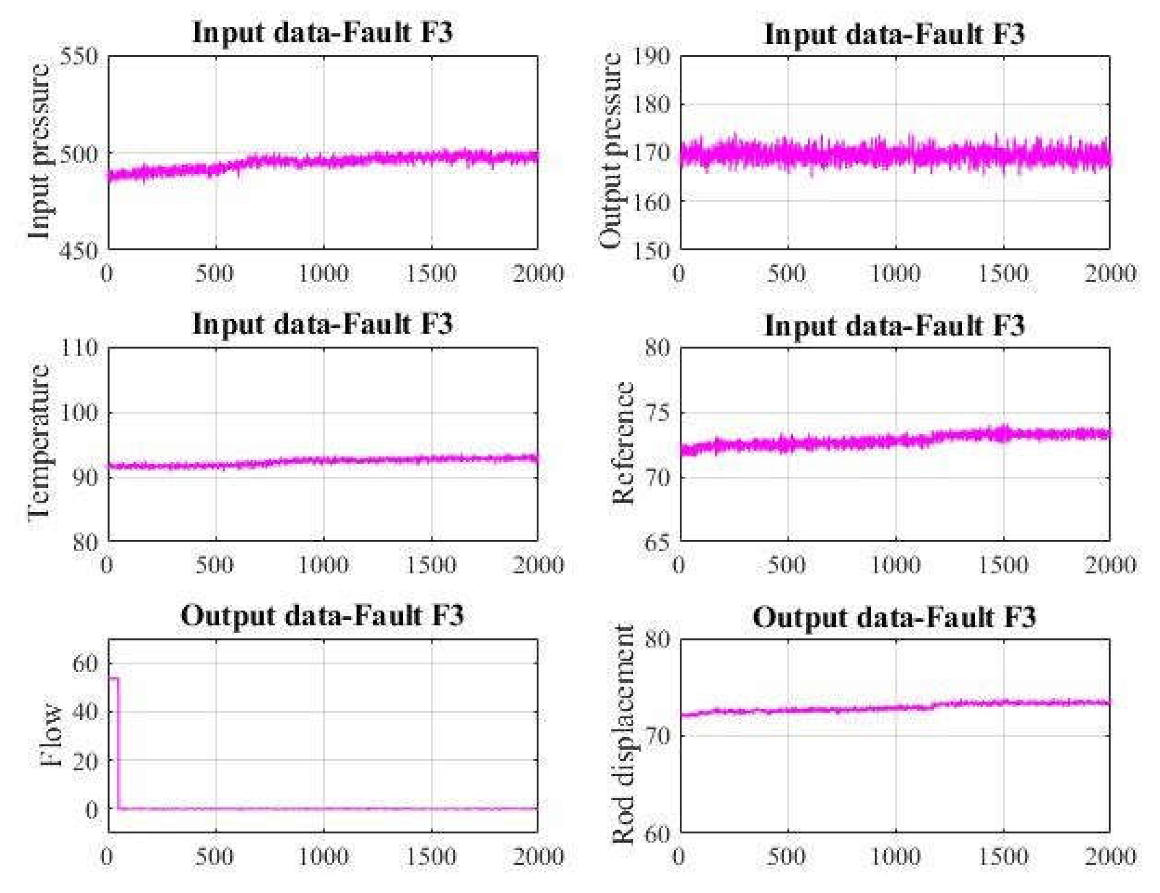
Figure 8.
Fault F1 detection.
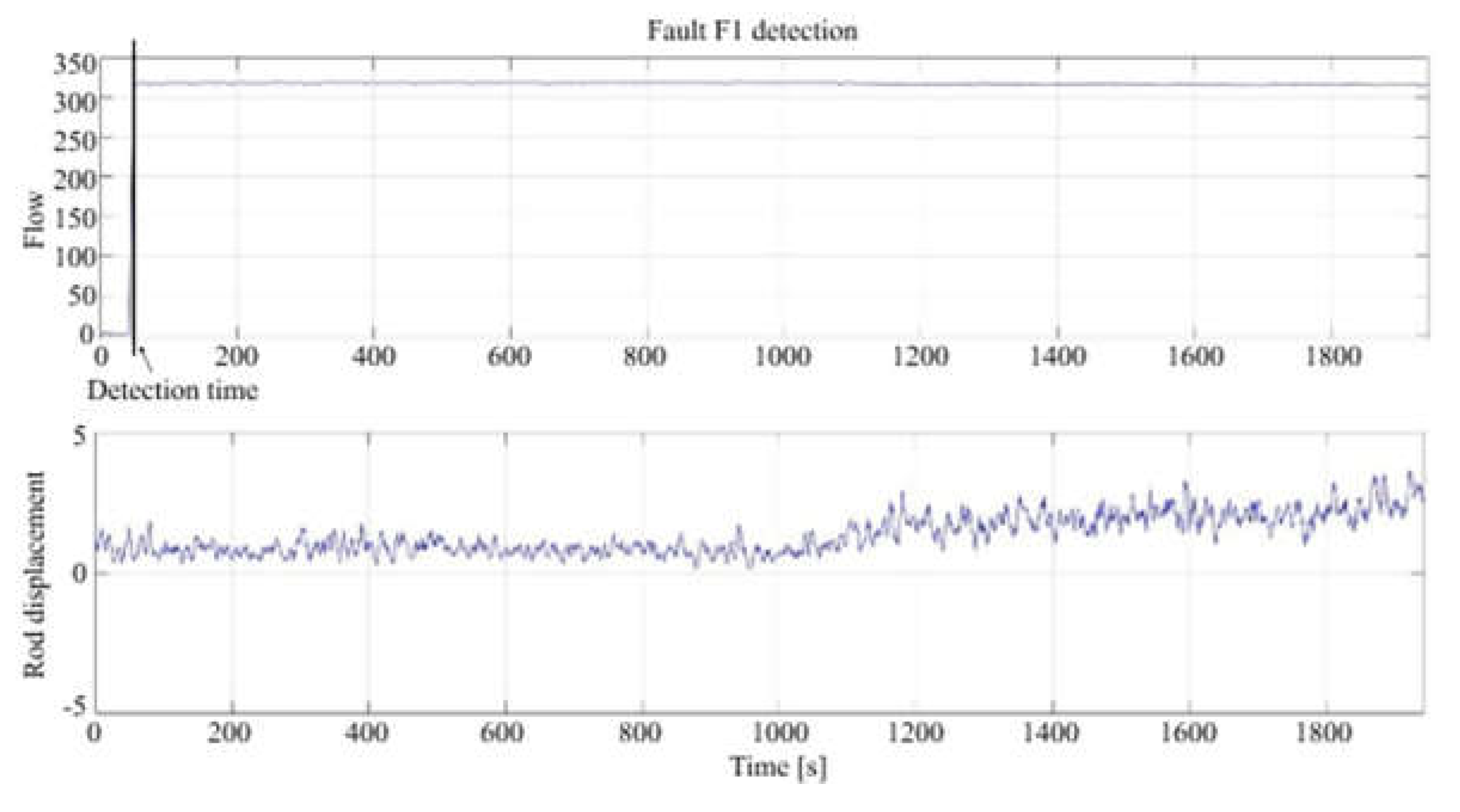
Figure 9.
Fault F1 isolation.
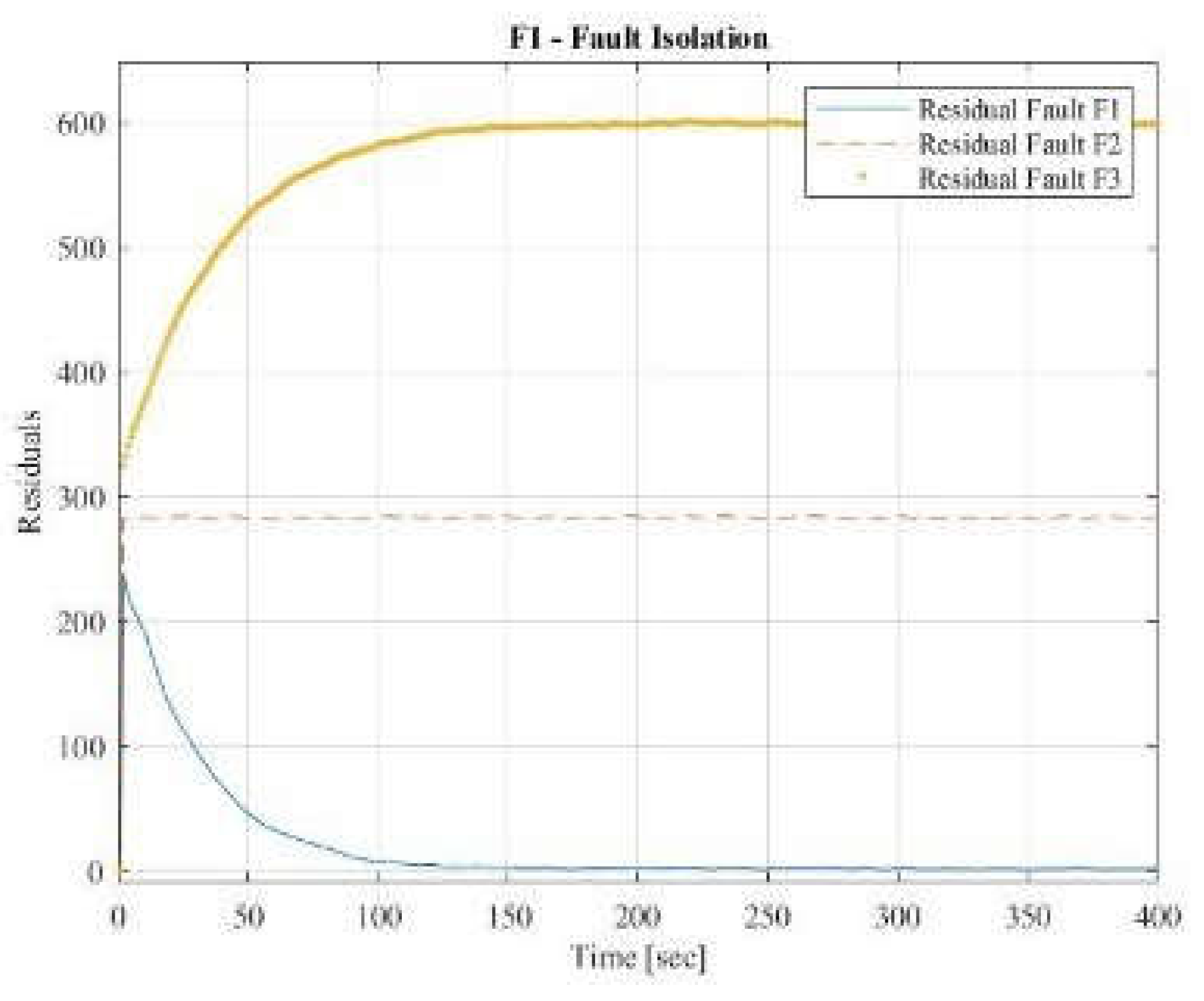
Figure 10.
Fault F2 isolation.
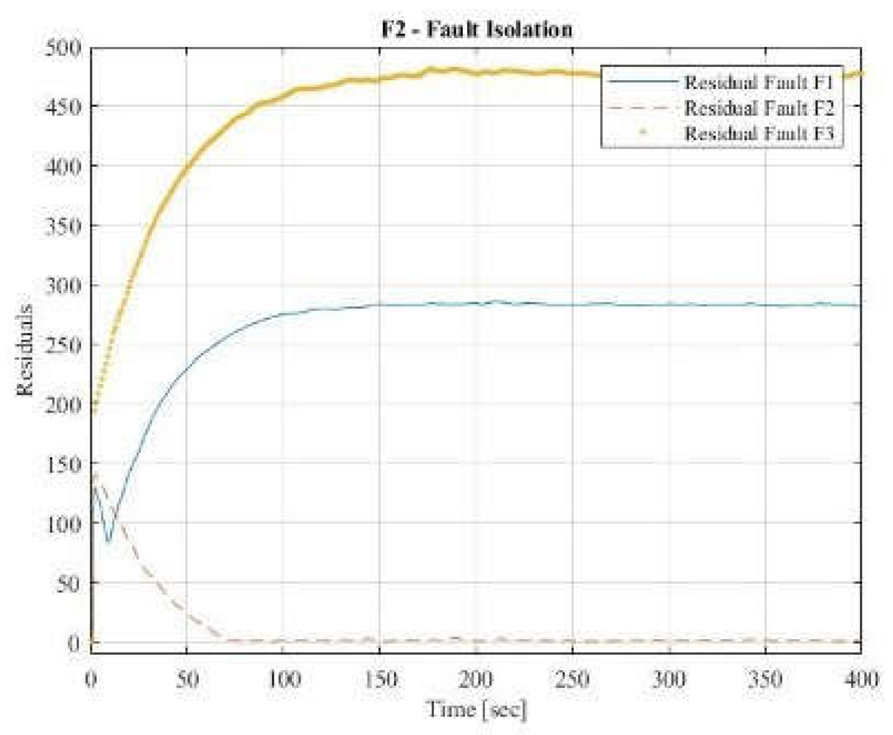
Figure 11.
Fault F3 isolation.
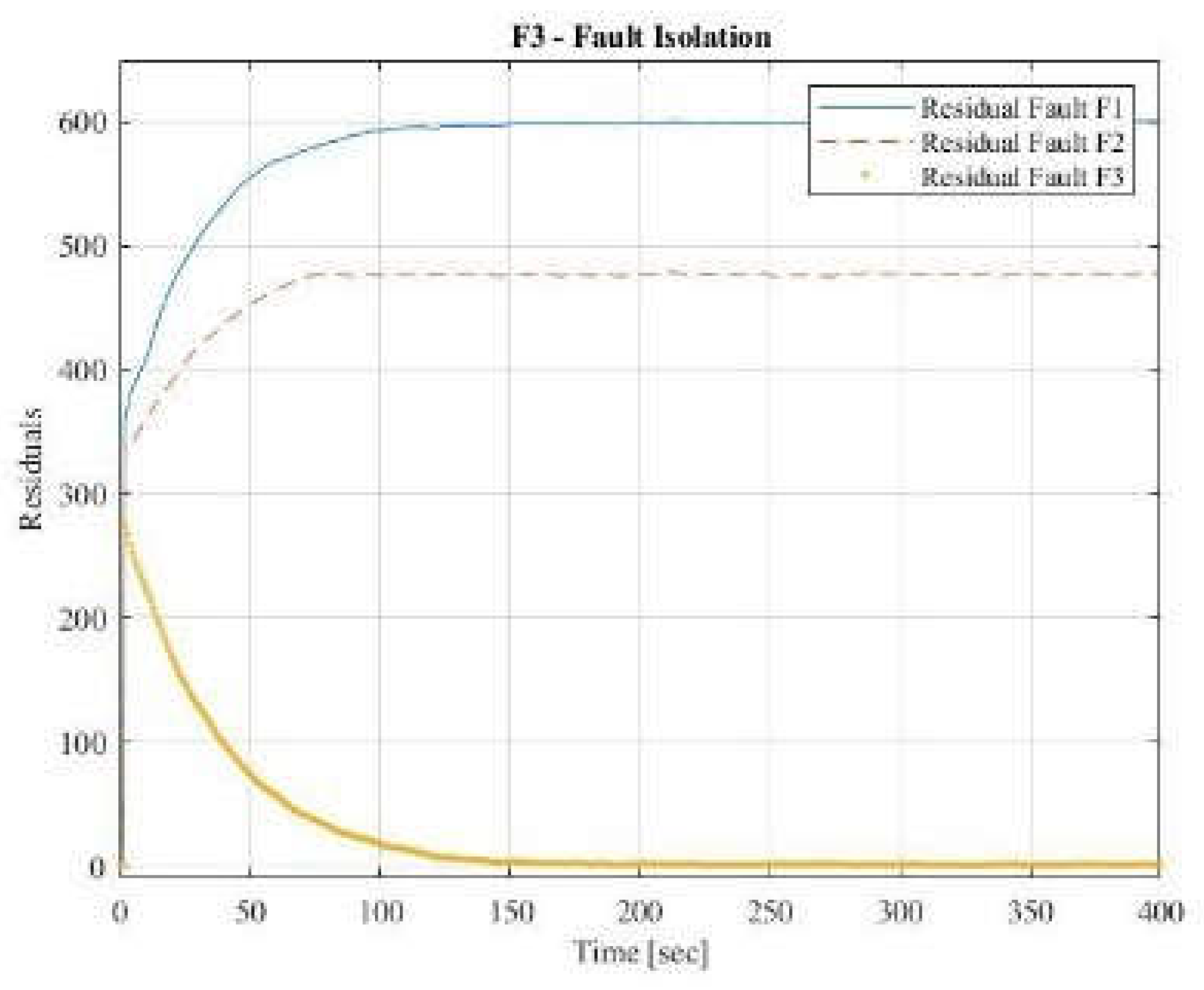

Table 1.
Faults description.
| Faults | Description |
|---|---|
| F1 | Valve clogging |
| F2 | Fully or partly opened bypass valve |
| F3 | Flow rate sensor fault |
Table 2.
Residual fault isolation (
| Input Faults | Fuzzy Model | ||
| F1 | F2 | F3 | |
| F1 | 483.91 | 8.0751e+04 | 3.5397e+05 |
| F2 | 7.9139e+04 | 186.77 | 2.2061e+05 |
| F2 | 3.5563e+05 | 2.2435e+05 | 761.06 |
Disclaimer/Publisher’s Note: The statements, opinions and data contained in all publications are solely those of the individual author(s) and contributor(s) and not of MDPI and/or the editor(s). MDPI and/or the editor(s) disclaim responsibility for any injury to people or property resulting from any ideas, methods, instructions or products referred to in the content. |
© 2024 by the authors. Licensee MDPI, Basel, Switzerland. This article is an open access article distributed under the terms and conditions of the Creative Commons Attribution (CC BY) license (http://creativecommons.org/licenses/by/4.0/).
Copyright: This open access article is published under a Creative Commons CC BY 4.0 license, which permit the free download, distribution, and reuse, provided that the author and preprint are cited in any reuse.


